Class vs. Identity: The Effect of Candidates’Race on the

Inequality-Redistribution Nexus∗

Konstantinos Matakos†

King’s College Londonkonstantinos.matakos@kcl.ac.uk

Dimitrios Xefteris‡

University of Cyprusxefteris.dimitrios@ucy.ac.cy

This draft: 18 October 2016

Abstract

Despite what the economic theory of democracy predicts, redistribution does not respond always to

rising inequality. In this paper we argue that redistribution reacts to changes in inequality, as long as

the economy is not overshadowed by non-economic issues during the elections. To this end we estimate

the race of candidates competing in all elections for U.S. state legislatures since 1980 and show that

when there are few (many) racially differentiated electoral contests, redistribution is (not) sensitive to

changes in inequality. That is, candidate heterogeneity crucially affects redistribution by raising the

salience of identity-related issues compared to class-related ones.

Keywords: inequality, redistribution, taxation, racial heterogeneity, candidate differentiation, U.S.

state legislatures.

JEL classifications: D63, D72, H20

∗We would like to thank participants in the following seminars and conferences for useful feedback and suggestions: King’sCollege London, London School of Economics, University of Cyprus, Erasmus University of Rotterdam, the 2015 EEA-ESEM Annual Congress, the Midwest Political Science Association 2016 Annual Meeting, the European Political ScienceAssociation 2016 Annual Conference, and the Royal Economic Society 2016 Annual Conference. We are grateful to ShaunHargreaves-Heap, Petros Milionis, Cecilia Testa, Laurent Bouton, Carlo Prato, Toke Aidt, Tolga Sinmazdemir, Marco Giani,Jim Snyder, Paola Giuliano, and Alberto Alesina for fruitful discussions and useful comments. We would also like to thankEleni Kostelidou, Antonios Matakos, and Danilo Freire for excellent research assistance. All errors remain ours.†King’s College London, Department of Political Economy, Strand building S.2.43, London WC2R 2LS, United Kingdom.‡University of Cyprus, Department of Economics, PO Box 20537, 1678 Nicosia, Cyprus.

1

1 Introduction

Economic theory of democracy (Downs 1957) predicts that as income inequality rises, taxation and

redistribution should increase (e.g., Meltzer and Richard 1981; Alesina and Rodrik 1994; Persson and

Tabellini 1994). This is because in a representative democracy framework, candidates want to be elected,

and, hence, they have to offer policies that somehow reflect the preferences of the majority of voters. When

inequality rises —that is, when the voter with the median income becomes poorer relative to the one with

average income—the majority of voters (voters whose income is below the average income) expects larger

utility gains from a greater redistribution. As a result, the theory predicts that, in the context of elective

politics with politicians that care about being (re)elected, an increase in income inequality should lead to

greater redistribution. Notice that this theoretical prediction regarding the positive relationship between

income inequality and redistribution relies only on the core assumption of rational choice theory: the

assumption that all actors of the game pursue their interests in an individually rational manner. The

intuition behind this idea is so strong and straightforward that Aristotle famously asserted that in a

democracy the will of the poor is sovereign because they are in majority.

Yet, despite the fact that this theoretical prediction is intuitive, empirical evidence from the U.S. as

well as from other advanced industrialized democracies does not validate it (e.g., Rodriguez 1999; Pecoraro

2014). While over the last couple of decades inequality has been increasing in most of the industrialized

world (Piketty and Saez 2003; Atkinson et al. 2011), redistribution —especially in the U.S.—did not rise.

In fact, if anything, it is declining (Figures 1.a and 1.b). As Rodriguez (1999) suggests, there seems to

be no link between rising inequality and increased redistribution in the U.S. Moreover, recent empirical

studies that extend their analysis beyond the U.S. (e.g., Karabarbounis 2011; Lupu and Pontusson 2011;

Pecoraro 2014) suggest a very weak relationship between inequality and redistribution.1 Hence, this

seemingly intuitive theoretical prediction lacks adequate empirical support. In fact, it has given rise to

the inequality-redistribution puzzle: If inequality is no longer a relevant determinant of redistributive

outcomes, then what determines redistribution or public good provision?

[Insert Figures 1.a and 1.b about here]

This evident lack of empirical support for such a straightforward theoretical prediction has prompted1Karabarbounis (2011) and Lupu and Pontusson (2011) find some cross-country evidence that suggest the existence of a

positive relationship between inequality and redistribution in a sample of OECD countries. Yet no such evidence exist whenone explores this relationship using within-country observations.

2

many observers —especially in light of the recent presidential race in the US and the Brexit vote in the

UK— to declare that the politics of class are no longer relevant: they have been replaced by a new

type of politics, those of (ethnic, racial, religious, or cultural) identity. In the literature, many scholars

have attempted to address this empirical puzzle. Most of them argue that there are other factors that

may be more important in explaining demand for redistribution than income inequality. For example,

Alesina et al. (1999) and, Alesina and Glaeser (2004) have proposed a link between the degree of voters’

ethnic heterogeneity and demand over redistribution. Alesina et al. (2001) attribute the differences in

redistributive outcomes between Europe and the U.S. to differences in overall ethnic heterogeneity of their

respective populations, while Alesina et al. (1999) provide some clear within-country evidence (using data

from U.S. urban counties and metropolitan areas) on the nature of this relationship.2 In all these studies,

the main argument is that, in societies where ethnic and racial heterogeneity is high, voters do not push

for extended redistribution (and public good provision) even if inequality is high. That is, in a society

where many ethnic and racial identities are present, voters might demand less redistribution out of the

perceived fear that their resources and income will be redistributed to members of an other ethnic or racial

group with which they do not feel close enough. This theory can explain, indeed, why societies with high

levels of inequality and ethnic fragmentation might redistribute less than societies with lower levels of

fragmentation but does not aspire to justify the weak relationship between inequality and redistribution:

ceteris paribus, an increase in inequality should lead to an increase in redistribution and public good

provision.

More recent studies (e.g., Karabarbounis 2011) argue that relatively richer voters have greater influence

in politics, and, hence, their interests are better represented. It may also be the case that relatively more

wealthy citizens tend to participate more in the political process. There is ample of evidence (e.g.,

Rosenstone and Hansen 1993; McCarty et al. 2006) that in many advanced democracies poor citizens

have lower turnout rates in elections. Other studies (e.g., Campante 2011) point to the role that special

interest groups have via campaign spending or media control in determining redistributive outcomes,

mainly in the direction of less redistribution and taxation irrespective of the recent trends in income

inequality.3 The overwhelming consensus in the literature, summarized in Persson and Tabellini (2003)

and Alesina and Glaeser (2004), appears to be that income inequality is not a significant determinant of

2Dahlberg et al. (2012) provide evidence on the relationship between ethnic heterogeneity and preferences for public goodprovision in Sweden while Padró i Miquel (2007) studies the effects of ethnic divisions on taxation policies and redistributionin non-democratic regimes.

3Prato (2016) shows that, in a Meltzer-Richard-Roemer framework with imperfect information about the state of theeconomy, subsidies to real estate ownership can produce an electorate that is systematically less favorable to redistributivetaxation.

3

redistribution. Simply put, the politics of class have become irrelevant.

This paper begs to differ; using data from U.S. state-wide elections for local legislative offi ces (State

House and State Senate), we present clear evidence that a positive relationship between income inequal-

ity (measured by the ratio of mean to median income) and redistribution (taxation) does, in fact, exist

regardless of how ethnically (or racially) heterogeneous a society might be. That is, we show that income

inequality is still a relevant —and perhaps the most important—determinant of redistributive outcomes.

As a result, this paper is the first to bridge the gap between the prediction of economic theory of democ-

racy —that as the median voter becomes poorer redistribution should increase—and the lack of empirical

support in its favor. At the same time, we show that the effect of inequality on determining redistributive

outcomes is conditioned on one key factor: the salience of non-economic issues (e.g., issues related to

race and ethnicity) during the electoral campaign. We find that, when identity-related issues are less

salient compared to class-related ones, then redistributive outcomes strongly depend on voters’economic

preferences and vice versa. Thus, our paper contributes to this long-standing liteature by uncovering a

new mechanism —one that operates in tandem with other mechanisms linking voters’preferences for re-

distribution with changes in ethnic heterogeneity—that connects issues related to race and ethnic identity,

and redistributive outcomes.

In order to do so, we focus on the process that generates policy outcomes in representative democracies,

and we show the existence of an innate tension between the observed level of redistribution and the salience

of non-economic matters, namely issues related to candidates’ immutable identity (e.g., ethnic, racial,

religious, or cultural) characteristics.4 In representative democracies, voters vote for candidates and not

directly for policies or levels of public good provision. That is, a candidate is essentially a bundle of policy

proposals (with regard to issues such as redistribution, immigration, etc.) and non-economic immutable

characteristics (such as race, ethnicity, religion, etc.). In other words, electoral competition might be

taking place in dimensions beyond economic concerns. Since voters care about the entire bundle, one

should not disregard the possible impact that these immutable characteristics can have on redistributive

outcomes. When electoral competition takes place in more than one dimension, we know that policy

outcomes do not necessarily have to reflect the preferences of the median voter in any given dimension,

including the economy (Plott 1967; McKelvey andWendell 1976). As a result, the sensitivity of candidates’

policy proposals to voters’preferences for redistribution —which, in turn, depend on inequality—might be

conditioned on the salience of non-economic issues such as race, ethnic identity, and religion relative to

4For example, Bursztyn et al. (2016) provide experimental evidence on the importance of identity and the trade-off thatvoters face between economic and non-economic issues.

4

economic ones during the electoral campaign (e.g., Lindbeck and Weibull 1987; Roemer 1999; Krasa and

Polborn 2012 and 2014; Bouton et al. 2014; Matakos and Xefteris 2016).

In attempting to provide an answer to the inequality-redistribution paradox, previous empirical liter-

ature studied the problem as a unidimensional one. Ethnic, racial, or identity heterogeneity was factored

into voters’preferences and determined their demand for redistribution and public good provision (e.g.,

Alesina et al. 1999; Alesina and Giuliano 2010), and the only policy outcome voters cared about was the

level of redistribution or public good provision. By explicitly focusing on how candidates’racial identity

heterogeneity can raise the salience of non-economic matters, we turn our attention to the supply side

of the problem instead.5 Consider, for example, the case where two competing candidates have identical

immutable characteristics. In this case, the economic dimension is more relevant in determining voters’

choices since identity issues like race are not salient. This should incentivize candidates to pander to the

median voter on the economic dimension, and, hence, conditional on candidates being identical, we should

expect that an increase in income inequality (that is, mean income rises relatively more than median)

should lead to greater redistribution.

On the other hand, when candidates have different immutable characteristics, a move towards median-

preferred redistributive policies does not deliver the same payoff to a candidate as in the case in which

candidates are identical. This is because when candidates have the same immutable characteristics, the

majority of poor voters will vote for the one who promises greater redistribution, even when the promises of

the candidates do not differ that much. In contrast, when candidates differ in race or ethnicity, the reaction

of poorer voters to the prospect greater redistribution need not be unanimous: Many of them may prefer to

stick with the candidate with whom they share common characteristics even if she promises less generous

redistribution. As a result, candidates who wish both to satisfy the voter with the median income (in order

to be elected) and special interest groups or constituencies that might prefer less or more redistribution

than the median voter (in order to be financed or due to honest ideological alignment with their interests),

should face weaker incentives to supply policies that reflect the redistribution preferences of the voter with

the median income when they compete against candidates with different immutable characteristics. The

dimensionality of the problem is no longer singular. That is, an increase in income inequality should

result, through this process, to an increase in redistribution when candidates are similar, while it should

have a smaller effect on redistribution —if any effect at all—when candidates are differentiated. When the

5We chose to focus on race instead of, say, religion because: a) it is not always easy to observe and thus measure acandidate’s religious affi liation, and b) candidates can strategically misrepresent the intensity and the importance of theirreligious identity, while this is harder, if not impossible, when it comes to their racial identity.

5

most salient issue in an electoral campaign is redistribution, candidates find it very diffi cult to ignore the

voter with the median income, thus implying a stronger link between inequality and redistribution.

To measure the relative salience of issues related to race and ethnicity, we focus on electoral contests

that took place between candidates of possibly different ethnic or racial backgrounds. Given the absence

of a comprehensive database that includes demographic information on race and ethnicity for all candi-

dates that contested state legislative elections in the U.S., we use, for the first time in the literature of

redistributive politics, a name-matching technique with Bayesian updating based on demographic data

provided by the US Census Bureau and compile a new data set that estimates the race of all candidates

competing in state-wide local legislative elections from 1979 to 2012. We are, therefore, able to construct

an index that captures the explicit degree of salience of issues related to race and ethnicity in the elections:

The fraction of state-wide electoral contests that were contested among candidates of different ethnic or

racial backgrounds, what we call differentiated candidates (following Krasa and Polborn 2012 and 2014),

for a given state in a given election year. Besides this methodological novelty, our empirical methodology

differs from past empirical literature in that it simultaneously introduces the following elements: a) We

use various different indices of income inequality in the same empirical framework to control for the fact

that redistribution might be driven by changes in relative inequality between different groups, b) we mea-

sure inequality using gross (before any deductions) annual earnings data, c) we use different measures of

redistribution (e.g., social transfers and effective income tax rate), and d) we conduct our analysis at the

sub-national level and exploit within-states variation in order to control for other important determinants

of redistribution that past literature has emphasized and which might vary across different countries (e.g.,

institutions, culture, electoral rules, etc.).6

Our findings suggest that once we take into account the salience of non-economic matters (such as

matters related to race and ethnicity), inequality has the expected effect (as in Meltzer and Richard 1981)

on redistributive outcomes. For example, suppose we start from a point where the mean and the median

income are the same (low inequality). We find that, in a given election year, when fewer than a quarter

of all state-wide electoral contests were contested between differentiated candidates —implying that the

electoral competition for the composition of the state’s legislature is characterized by low levels of racial

or ethnic salience7— a one-standard-deviation increase in income inequality (measured as the ratio of

mean-to-median income) is associated with almost a doubling of the effective (state) tax rate. In fact, the

6For an illustration, see Iversen and Soskice (2006), Alesina and Glaeser (2004), Alesina and La Ferrara (2002), andAlesina and Giuliano (2010).

7 In U.S. states, it is the local legislature (State House and Senate) that has control over a given state’s tax and redistributivepolicies.

6

effective state tax rate increases from 5.5% to 9%, almost four percentage points. That is, inequality is still

a relevant, and perhaps the most important, determinant of redistributive outcomes. But when greater

than a quarter of electoral contests (within a given state) are contested among candidates of different

racial and ethnic background (differentiated candidates), then redistribution and taxation appear not

to respond in changes in inequality. The salience of race rises, and non-economic issues dominate thus

eliminating any effect on redistributive outcomes that inequality might have. Therefore, our analysis

shows that the intuitive theoretical prediction regarding the positive relationship between inequality and

redistribution is, in fact, in line with empirical evidence, once we take into account the existence of other,

possibly more salient, dimensions of political competition.

In what follows, we provide a more detailed presentation of the mechanism that was briefly described

above in Section 2. We then describe our data set especially, how we estimated the ethnic characteristics

of all candidates running for U.S. state legislative elections since 1979, our econometric specification, and

our main results in Section 3. Finally, we discuss the implications of our findings and possible extensions

—along with some final remarks—in Section 4.

2 Theoretical background

In representative democracies’frameworks, voters may defend their interests only by electing candidates

whose policy platforms align with theirs. It is, therefore, natural to expect that candidates who propose

popular policies are more often elected to offi ce, and, hence, implement policies that, to some degree, match

society’s preferences (Downs 1957). If we focus on the easily quantifiable policy issue of redistribution,

the above suggest that the level of redistribution in a representative democracy society should reflect

to a large extent the preferences for redistribution of the median voter. The larger the mean-to-median

ratio, the more redistribution the median voter desires, and, thus, the larger the redistribution we should

observe (Meltzer and Richard 1981).

Hypothesis 1 (Meltzer and Richard 1981) The relationship between income inequality (measured by

the mean-to-median ratio, y/y50) and redistribution is positive.

Unlike direct democracy frameworks in which voters vote directly for a policy, in representative democ-

racies voters vote for candidates who, in turn, decide on policies such as redistribution. Since candidates

7

care about winning elections and about promoting the goals of certain interest groups to which they

belong or by which they are funded, they face the following problem: On the one hand, they wish to

secure as many votes as possible, and, hence, they have incentives to promise policies that are appealing

to the median voter. On the other hand, they also want to satisfy the interest groups and the con-

stituencies that they represent (see, for example, Besley and Preston 2007). Because popular (that is,

the median-preferred) policy platforms need not coincide with the ideal policies of the special interest

groups, candidates’optimal behavior should be to locate somewhere in between what the interest groups

that support them desire and what the society (that is, the median voter) wants. Note that this holds

true particularly in the case of redistribution and taxation. A candidate essentially knows that by moving

towards the median’s most preferred policies she gains support from the voters and loses support from

the special interest groups that she is supposed to represent.

So, what determines how strong the incentives must be for a candidate to ignore the requests of interest

groups and instead satisfy the median voter? Both common wisdom and academic analyses (e.g., Citrin

et al. 1990; Sparks and Watts 2010; Boudreau et al. 2014; Ahler et al. 2015) strongly suggest that voters

decide which candidate to support not only by taking into account the candidates’policy proposals vis-

a-vis redistribution (or social spending and taxation) but also on the basis of candidates’identities. That

is, voters take into account candidates’immutable characteristics (such as race, ethnicity, or religion). It

is, therefore, reasonable to expect that in electoral contests between two candidates with similar racial,

ethnic, or religious identities, the positions of the candidates on the policy issues should be the only

relevant factor in determining the electoral outcome. In such cases, candidates’incentives to pander to

the median are very strong as identity plays no role, and voters vote only on the basis of the candidates’

policy platforms. In contrast, when elections are contested by candidates with heterogeneous identities

(we call these candidates and their contests differentiated), candidates’non-policy characteristics might

have a large effect on the electoral outcome. In these differentiated contests, candidates’racial or ethnic

characteristics might have a large effect on the electoral outcome, and, hence, candidates can now afford

to pander more to special interests and to the constituencies that they represent.

It is exactly in these differentiated contests that the identity characteristics of the candidate become

a salient issue as each candidate is de facto associated with a certain group of voters. As a result, her

incentive to move toward the median voter’s most preferred policy is mitigated; such a move now brings

a relatively small benefit since in such elections voters will also vote on the basis of candidates’identity.

That is, we should observe that the policy outcomes of elections between candidates of identical racial or

8

ethnic identities better represent the societies’preferences compared to the policy outcomes of elections

between differentiated candidates. If we focus again on the issue of redistribution, the above suggest

that rising inequality, an increase in the ratio between mean and median income, should lead to more

redistribution (that is, higher taxation and social spending) when elections are between candidates of the

same racial or ethnic backgrounds. In this case, both candidates have strong incentives to pander to the

median voter who is becoming relatively poorer and demands more redistribution. But when elections are

contested by differentiated candidates, inequality should have little (if any) explanatory power regarding

redistribution and taxation. In such cases, candidates base their electoral success on their identity and not

on proposing redistributive policies that attempt to pander to the median voter. As a result, conditional

on a significant amount of electoral races being contested by differentiated candidates, we should expect

to find that the effect of inequality on redistribution is negligible. Racially or ethnically differentiated

candidates can now afford to pander to special interest groups as far as redistribution is concerned.8 This

suggests that as the amount of minority candidates increases, inequality becomes an even less relevant

determinant of taxation and redistribution. We have to stress, though, that our argument does not imply

that when there are many minority candidates, redistribution is smaller; it merely suggests that in such

contexts, redistribution is less responsive to changes in inequality.

We can summarize the developed idea using the following statement.

Hypothesis 2 (Conditional) The effect of income inequality (measured by the mean-to-median ratio,

y/y50) on redistribution is: (a) positive when a suffi ciently large number of electoral races is contested

by candidates of the same racial background (that is, matters related to race are not very salient), and

(b) weakens and ceases to be significant when a large number of electoral contests is contested by racially

differentiated candidates (that is, matters related to race are very salient).

Notice that the above arguments are perfectly in line with recent findings of formal political economics’

literature. Indeed, Krasa and Polborn (2010; 2012) analyze theoretical models in which two candidates

with different fixed characteristics compete by making proposals regarding a number of policy issues,

and they show that the degree of similarity of candidates’fixed characteristics is crucial in determining

candidates’policy proposals. In particular, Krasa and Polborn (2014) interpret these fixed characteristics

as candidates’social identities, and show that the degree of identity-differentiation between candidates

8Note that this statement is unconditional on the overall level of ethnic or racial heterogeneity within a constituency.That is, we expect this statement to be true irrespective of the effect that overall heterogeneity might have on redistribution,in line with Alesina and Glaeser (2004).

9

influences the candidates’ choices as far as economic policy is concerned. Hence, our main hypothesis

is grounded on widely-accepted views regarding the determinants of candidates’ choices, and does not

contradict other predominant determinants of redistribution (e.g. voters’ethnic heterogeneity).

3 Data and Econometric Specification

In order to test these hypotheses, we use data on redistribution and inequality from U.S. states using

resources provided by the U.S. Census Bureau, the Bureau of Economic Analysis (BEA), and the Bureau

of Labor Statistics (BLS). Our unit of analysis for all observations is the state-year. The reason we

perform our analysis at the state level is twofold. First, it guarantees that we get suffi cient within-year

variation since there is only one yearly observation of realized redistribution (or taxation) at the federal

level, but each state sets each own tax rate. Second, while the state tax rate is a non-negligible fraction

of one’s income (in our sample it is on average 5% of total income), and, moreover, it exhibits suffi cient

within-state variation over time, it is not high enough to trigger significant cross-state migration for tax

purposes. Furthermore, focusing on the U.S. has two additional advantages: We can get data on the

distribution of income and other economic variables, and we can get those data at the yearly level from

1979 until today via the Current Population Survey’s (CPS) Annual Earnings Files that are stored at the

NBER data base and are the most reliable source of such information. Finally, identity politics, especially

with respect to race and ethnicity, have long been a defining characteristic of the political environment

and competition in the U.S., both at the local and at the national level. As a result, we will investigate

the validity of our hypotheses focusing exclusively on the U.S. at the sub-national level in the spirit of

Alesina et al. (1999).9

3.1 Baseline specification

Before exploring the full richness of our new data set, we first estimate a more basic specification in the

spirit of Alesina et al. (1999) and Karabarbounis (2011):

Ts,t = β0 +τ=∑τ=1

Ts,t−τ + β1

(yy50

)s,t

+ β2ERFs,t + β3ERFs,t ∗(

yy50

)s,t

+X′s,tγ + αs + λt + εs,t (1)

9A number of previous studies that examined the interplay between class and (ethnic) identity politics focused on cross-country evidence (e.g., Alesina and Sacerdote 2005; Lupu and Pontusson 2011). Alesina et al. (1999) conducted the seminalanalysis on the relationship between voters’ ethnic heterogeneity and public good provision at the sub-national level, yettheir mechanism, as we will show in the section that follows, is different than ours.

10

where Ts,t is the effective state tax rate in state s in year t, income inequality is measured as the ratio

of mean (pre-tax and any deduction) income (y) to the median one (y50), and ERFs,t is the index of ethnic

and racial fragmentation in state s in year t, constructed identically to the index of ethnic fragmentation

used in Alesina et al. (1999). In other specifications, we also employ alternative popular measures of

inequality, which we will describe in detail in the following section. Other controls include economic

(e.g., the female labor force participation rate, unemployment rate, and log of State GDP per capita) and

political (e.g., partisan control of the local legislature and political alignment of the governor) variables

and state and election year fixed effects. In some specifications, we also use lags of our dependent variable.

Below, we describe in more detail how we operationalize the main variables used in our estimation.

Moreover, our empirical analysis looks carefully at the role that ethnic and racial heterogeneity might

have on the demand for redistribution, as suggested by Alesina et al. (1999) and Alesina and Glaeser

(2004). For this reason, our analysis takes into account the possibility that there might be an interaction

between income inequality and non-economic determinants of redistribution, which were found to have

an effect on redistributive outcomes and public good provision (Alesina et al. 1999). That is, according

to this approach, it can be the case that a given increase in income inequality should lead to a relatively

larger increase in the demand for redistribution when the society is more homogeneous (less fragmented)

compared to the case where the society is more heterogeneous. In the latter instance, we should expect

a smaller increase in the demand for redistribution. Hence, we have also interacted the index of ethnic

and racial fragmentation with the measure of inequality that we employ, as in Karabarbounis (2011), in

order to control for Lind’s (2007) conjecture that only in less heterogeneous and less fragmented societies

does inequality increase redistribution.

3.1.1 Variable definitions and description

Dependent variable Following most of the literature, we measure redistributive outcomes using the

effective state tax rate and the level of social spending at the state level. We compute the state effective

tax rate in percentage terms as the ratio of the state’s total per capita tax receipts over (per capita) income

at the state level. In addition to the total effective tax rate, we also compute the effective (individual,

corporate, and total) income tax rate, and the effective property tax rate. As before, the denominator

is the per capita total income at the state level and the numerator is the state’s individual, corporate,

property, and total income tax receipts (per capita). We get our data for tax receipts (total and itemized)

and income (per capita) at the state level from the U.S. Census Bureau and the BEA’s regional data base.

11

In addition to the effective state tax rate, we also measure redistributive outcomes using the state

social transfers rate (in percentage terms) defined as the ratio of total (per capita) state social transfers

over (per capita) income at the state level, using again data from the regional data base of the BEA for

social transfers and income at the state level.10

Inequality To operationalize the measurement of income inequality, we use standard measures from

the literature. While data on the Gini, Theil, and Atkinson indexes of income inequality are available at

the state level, as most of the recent literature suggests (e.g., Rodriguez 1999; Lupu and Pontusson 2011;

Pecoraro 2014) these measures do not capture changes in inequality that are politically relevant.11 That

is, they are not very informative on the relationship between median and mean incomes, which is what

determines redistributive outcomes according to most models. For this reason, in addition to using some

of the standard measures of inequality presented above, we focus our analysis on three measures that

are, in our view, more relevant and robust determinants of redistribution, taxation, and social spending:

a) the mean-to-median ratio of gross (pre-tax) individual earnings (y/y50); b) the relative difference of

mean to median gross (pre-tax) income difference ((y−y50)/y); and c) the skewness of the distribution of

gross individual earnings. In order to compute the mean (y) and median (y50) gross income at the state

level, we use the data on gross (before taxes and any deductions) annual earnings from the CPS Annual

Earning Files, which contain detailed information on annual earnings since 1979.

Moreover, in addition to the above measures of income inequality, we also use the P90 to P50 ratio

(y90

y50) or the ratio of the income of the 90th percentile of the income distribution (top decile) over median

income; the P50 to P10 ratio (y50

y10) or the ratio of median income over the income of the bottom decile;

and the P90 to P10 ratio (y90

y10), or the ratio between the income of the 90th percentile (top decile) over

that of the 10th percentile (bottom decile). We do so because many scholars (e.g., Karabarbounis 2011;

Lupu and Pontusson 2011) discuss the possibility that what matters most is the relative distance of the

middle-class voters, or those who earn the median income, from the top and bottom deciles of the income

distribution. Their main argument is that since the median voter is decisive with her preferences reflected

by the democratic process, the middle class aligns with the rich elites (top decile) as the ratio of the

median over top income is increasing. By contrast, the middle class aligns with the poor —and demands

more redistribution when the ratio of their income over the bottom decile income is shrinking. That is,

the closer the middle class feels to the poor, the more redistribution it prefers and vice versa. As a result,

10Data for social transfers are available starting in 1997 at the state level.11Despite this, we show in the appendix that our analysis is robust to alternative measures of inequality.

12

controlling for those measures of inequality will allow us to exclude this argument from being a possible

explanatory factor.12

Racial (ethnic) heterogeneity Following Alesina et al. (1999), we compute the index of racial (ethnic)

heterogeneity in a way analogous to their computation of the index of ethnic fractionalization. That is,

we compute:

Ethnic & Racial Fragmentations,t = ERFs,t = 1−∑

i(ri,s,t)2

where ri,s,t is the share of racial (or ethnic) group i in state s in year t. This index is the opposite

of a Herfindahl-Hirchman index and takes values from zero to one, where zero means no heterogeneity

(e.g., the whole population belongs to a single racial or ethnic group). A value of one, on the other hand,

implies extreme heterogeneity (e.g., every single individual belongs to a separate racial or ethnic group).

In order to compute the index, we follow previous literature to split the population in four distinct groups,

using the categories provided by the U.S. Census Bureau: whites (non-hispanics), blacks (non-hispanics),

Hispanics, and Asians and pacific islanders.13 In the data appendix, we provide detailed information on

how we have constructed this variable using micro-data from CPS Annual Earnings Files. In Figure 2,

we present the variation of the main variables of interest (effective tax rate, mean-to-median ratio, ERF

index) across states and over time.

[Insert Figure 2 about here]

Other variables We also employ a series of economic and political variables as controls in our estima-

tion. In particular, we use the average real income per capita at the state level and the real gross state

domestic product per capita (retrieved from the regional accounts data base of the BEA), the unemploy-

ment rate and the female labor force participation rate (from the regional accounts of the BLS), a binary

variable indicating partisan or split control over both chambers of the state’s legislature (State House

and Senate) taken from the National Conference of State Legislatures (NCSL), and, finally, a variable

indicating the political affi liation of the sitting governor.12We provide a detailed overview of how we constructed each of those measures in the data appendix.13Up until the early 2000s, those four categories were the only ones asked in the Census Current Population Surveys.

In years following 2001, survey respondents were given the option to self-identify using a much richer set of options (alsoallowing a person to choose more than one category). Yet for reasons of consistency throughout the whole sample, we restrictattention into those four categories, although the index does not vary dramatically if one is to incorporate a more (less)detailed break-down.

13

3.1.2 Results

Table 1 presents the results of the baseline specification. Our estimates are consistent with previous

findings: Inequality (measured in a variety of different ways) does not seem to be an important determinant

of redistributive outcomes (and, in fact, it always fails to be statistically significant at the 5% level).

However, we find some support for the hypothesis that racial and ethnic heterogeneity is negatively

associated with redistribution, as previous studies have found (e.g., Alesina et al. 1999; Alesina and

Glaeser 2004). That is, the results of the standard approach —one that does not take into account the

role that candidates’ racial identity might play—are consistent with previous findings in the literature

that inequality does not lead to more redistribution. Moreover, the introduction of a lagged dependent

variable and other controls does not change the general picture. As a result, in the section that follows we

introduce a measure of the degree of salience of issues related to race and identity: the share of electoral

contests (in a given state during a given election) that were contested between candidates of different

racial or ethnic backgrounds. Before presenting our results, we demonstrate in some detail how we have

estimated candidates’racial and ethnic identity.

[Insert Table 1 about here]

3.2 Candidate differentiation

As shown in Table 1, our results do not differ substantially from previous findings in the U.S. context (e.g.,

Alesina et al. 1999). At first glance, inequality seems to play little role, if any, in determining redistributive

outcomes while ethnic and racial heterogeneity seem to be negatively correlated with redistribution. Yet

the specification of equation (1) completely ignores the mechanism that we have put forward in Section 2:

Inequality is an important determinant of redistributive outcomes when economic matters are relatively

more salient than matters of race and ethnic identity. Therefore, in the section that follows we do

exactly this and construct an index that attempts to proxy the relative salience of issues related to

race and identity during an electoral campaign. In order to do so, we use data on each individual

candidate (winner and loser) who contested any election for a local legislative offi ce at the state level

since 1979, and we estimate the state-wide proportion of electoral contests that were contested between

candidates of different racial backgrounds.14 We get information for each individual candidate from the

14Here it is, perhaps, necessary to explain why we have chosen to aggregate this information at the state level instead ofperforming our analysis at the most disaggregated level possible: a state’s electoral districts. There are important technical

14

State Legislative Election Returns (1967-2010) data set, compiled by the Inter-university Consortium for

Political and Social Research (ICPSR 34297-v1) led by the University of Michigan (Klarner et al. 2013).

We also supplemented this information using data from the U.S. Census Bureau. In the section that

follows, we describe our estimation technique in detail.

3.2.1 Variable construction: A Bayesian approach

In order to measure the proportion of electoral contests between racially differentiated candidates for a

given state and election year, one ideally needs to have data on the racial identity of all competing candi-

dates. Such comprehensive data for state legislative offi ces are not readily available. There are numerous

candidates for state legislative offi ces, and with the exception of recent elections during which many can-

didates promote their campaigns on the internet, their personal data (such as their race, ethnicity, and

religion) are diffi cult to retrieve from their own promotional materials. Indeed, certain characteristics of

past elected candidates might be found in the local press, but information about non-elected candidates

is scarce at best. Notice that in order to measure the proportion of differentiated electoral contests,

information both about the winners and the losers is absolutely necessary.

So, how do we proceed? In order to create a reliable and econometrically admissible and consistent

measure of candidate differentiation, we employ the estimation approach described below.

Step 1. We use the ICPSR State Legislative Election Returns data set (Klarner et al. 2013) which

contains detailed information on all candidates that competed in elections for state legislative offi ces in

all U.S. states from 1967 to 2010.15 This data set contains personal information for more than 150,000

candidates, including surnames, given names, state, electoral district, offi ce they run for, election year,

and other variables of interest. However, it does not include the race of each candidate.

Step 2. Next, we match the surname of each candidate with the racial distribution of U.S. citizens

barriers that make such analysis impossible. First, note that the boundaries of a state’s local electoral districts (that is, localcongressional districts) are not constant over time and, most importantly, they do not coincide with the boundaries of thecounties —which is the smallest reference unit for the US Census—simply because of gerrymandering: some counties containmultiple electoral districts and vice versa. But, even if one wanted to —painstakingly— identify which segments of countiesbelong in a particular electoral district, then it is absolutely necessary to work with micro-level Census data in order toidentify exactly which voters in a given county belong to one or another electoral district. Simply put, data aggregated at thecounty level will not be suffi cient to perform such an analysis. Unfortunately, the US Census Bureau embargoes the releaseof micro-level data with county identifiers for a certain period of years: the latest available micro-level data with full countyidentifiers are from 1960 and, hence, they cannot be used in our analysis. As a result, it is not possible for us to construct acomplete set of socio-demographic and economic variables (such as measures of inequality that require the full distributionof incomes in a particular unit of analysis) that are necessary for our analysis.15 In order to match our data from CPS’s Annual Earnings Files, we restrict attention to the period from 1979 on.

15

bearing this surname. For example, the racial distribution of U.S. citizens bearing the surname Smith is

the following: 73.35% are white, 22.22% are black, and 4.43% belong to other racial groups. We have

data for the 10,000 most popular surnames in the U.S. population from the U.S. Census Bureau. As a

result, not every candidate is matched with a racial distribution: All told, about 120,000 of the candidates

in the data set are assigned a racial distribution. Inspection of the data set shows that this matching is

quite constant over time. The percentage of candidates matched with a racial distribution varies very

little between the years. The same pattern is also observed at the state level.

Step 3. We update the racial distribution assigned to each candidate in order to take into account

the state- and year-specific racial distribution obtained from the CPS, using a Bayesian approach. This

is absolutely necessary since, if we only know that a candidate is named Smith, then we can correctly

assign him a probability 73.35% that he is white. But if we additionally know that this candidate is from

Maine, where white population represents the 94.4% of the total as opposed to 77.35% countrywide, then

we should assign a larger probability of being white to that candidate. Since the racial distribution of

the population of a state does not remain constant over time, we need to take into account state- and

year-specific racial distributions that are available from 1979 on a yearly basis in order to improve our

estimates. Consider that wi is the probability that a candidate with surname i is white given the primary

matching described in step 2. Then, following a Bayesian approach, the probability that a candidate with

surname i is white, given that this candidate competes in an electoral race in state s and in year t is:

wis,t =wi

w×ws,t

wi

w×ws,t+ 1−wi

1−w ×(1−ws,t)

where w is the countrywide percentage of whites in the year corresponding to the year of the original

racial distributions, and ws,t is the percentage of whites in state s and in year t.

To see the intuition behind this update, consider the example that follows. In a country at time t,

we have: a) m men and f women, with m < f , and b) certain individuals are named Billie, a share

bm of them are men and a share bf of the are women, with bm + bf = 1. Moreover, we denote by b

the probability that a randomly chosen individual is named Billie and by bm (bf ) the probability that a

randomly chosen man (woman) is named Billie. Notice that the latter are conditional probabilities and

hence bm = bm×bm/(m+f) and b

f = bf×bf/(m+f) .

Now assume that we randomly choose a woman out of the original women sub-population, and we

clone her (the cloning process creates identical individuals with identical names); and that we do this until

16

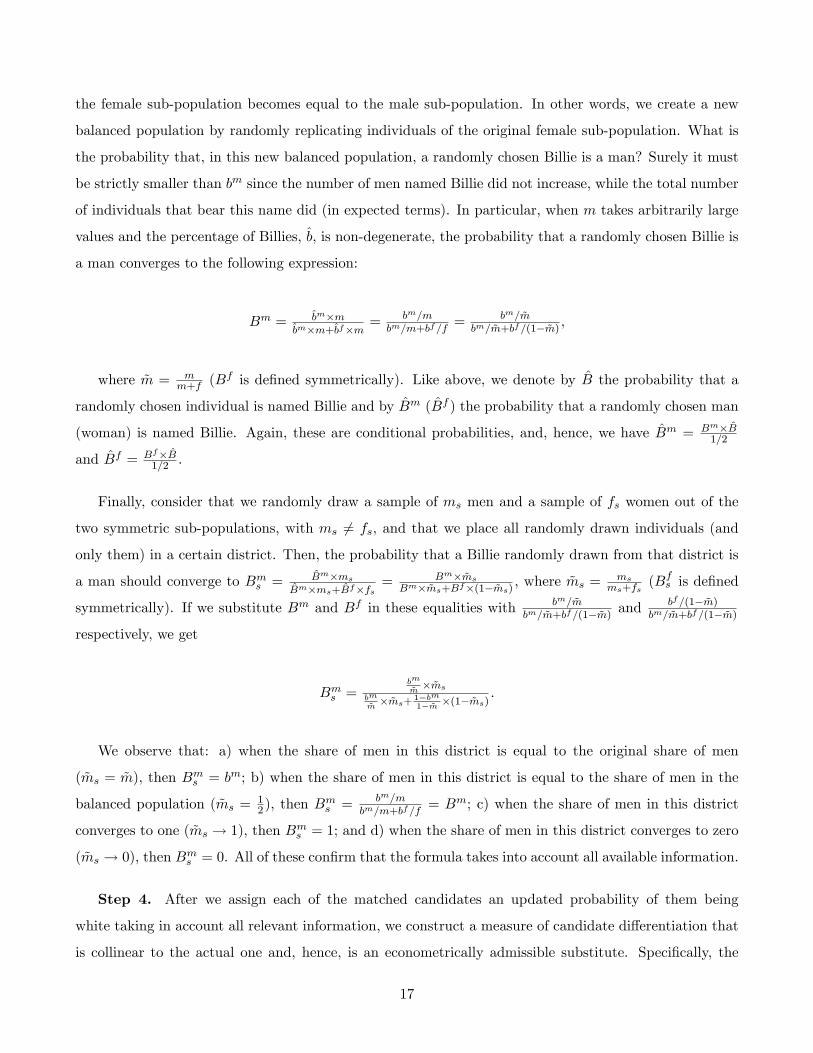
the female sub-population becomes equal to the male sub-population. In other words, we create a new

balanced population by randomly replicating individuals of the original female sub-population. What is

the probability that, in this new balanced population, a randomly chosen Billie is a man? Surely it must

be strictly smaller than bm since the number of men named Billie did not increase, while the total number

of individuals that bear this name did (in expected terms). In particular, when m takes arbitrarily large

values and the percentage of Billies, b, is non-degenerate, the probability that a randomly chosen Billie is

a man converges to the following expression:

Bm = bm×mbm×m+bf×m = bm/m

bm/m+bf/f= bm/m

bm/m+bf/(1−m),

where m = mm+f (B

f is defined symmetrically). Like above, we denote by B the probability that a

randomly chosen individual is named Billie and by Bm (Bf ) the probability that a randomly chosen man

(woman) is named Billie. Again, these are conditional probabilities, and, hence, we have Bm = Bm×B1/2

and Bf = Bf×B1/2 .

Finally, consider that we randomly draw a sample of ms men and a sample of fs women out of the

two symmetric sub-populations, with ms 6= fs, and that we place all randomly drawn individuals (and

only them) in a certain district. Then, the probability that a Billie randomly drawn from that district is

a man should converge to Bms = Bm×ms

Bm×ms+Bf×fs= Bm×ms

Bm×ms+Bf×(1−ms), where ms = ms

ms+fs(Bf

s is defined

symmetrically). If we substitute Bm and Bf in these equalities with bm/mbm/m+bf/(1−m)

and bf/(1−m)bm/m+bf/(1−m)

respectively, we get

Bms =

bm

m×ms

bm

m×ms+

1−bm1−m ×(1−ms)

.

We observe that: a) when the share of men in this district is equal to the original share of men

(ms = m), then Bms = bm; b) when the share of men in this district is equal to the share of men in the

balanced population (ms = 12), then B

ms = bm/m

bm/m+bf/f= Bm; c) when the share of men in this district

converges to one (ms → 1), then Bms = 1; and d) when the share of men in this district converges to zero

(ms → 0), then Bms = 0. All of these confirm that the formula takes into account all available information.

Step 4. After we assign each of the matched candidates an updated probability of them being

white taking in account all relevant information, we construct a measure of candidate differentiation that

is collinear to the actual one and, hence, is an econometrically admissible substitute. Specifically, the

17

probability that the two candidates16 are racially differentiated in district d of state s and in election year

t, is defined by:

Pd,s,t = wis,t(1− wjs,t) + wjs,t(1− w

js,t).

Strictly speaking, this is not the probability of an electoral contest being differentiated, but the

probability that a race is between a white and a non-white candidate. As a result, it underestimates the

actual probability that a race is between candidates of different races, making our approach a conservative

one. A more detailed measure would be more sensitive in fluctuations in the exact percentages of smaller

racial groups. This is quite problematic as such groups are treated differently throughout our sample

period. For example, in the early 1990s a new category of racial identification (Asian/Pacific islander)

was added to the previously existing three (black, white, other); in the mid-1990s an additional category

was added (Native American).17 Hence, the safest and most inter-temporally homogeneous approach is

to focus on a simple division between a candidate belonging to the majority group (white candidates) and

to a minority one (all other candidates).

Step 5. Electoral contests for state legislatures take place at the district level. That is, in state s

and in year t, we have as many electoral races as the electoral districts of that state s. If for a state s

in election year t we have suffi cient data to measure the probability of a differentiated (heterogeneous)

contest in districts that belong to the set Ns,t —the set of all electoral districts within a state that did not

have a candidate running unopposed—then the share of differentiated (heterogeneous) contests should be

approximated by:

Ps,t =

∑d∈Ns,t Pd,s,t

#Ns,t.

16 In the initial sample about 20% of the contests involved the incumbent running unopposed. We have, thus, removedthose cases from the sample we used to estimate our variable, since in those cases our variable has no meaning. We havealso removed from our sample a very small amount of candidates that received less that one percent of the vote. Thoseare fringe candidates, and, hence, they should not have any effect in influencing the salience of issues during the electoralcampaign. After removing a small fraction of entries from candidates that competed in MMDs (in multi-member districtsthe idea of pairing candidates competing against each other for one seat is quite problematic) as well, we were left only withelectoral races the vast majority of which (99% of total) involves a two-candidate contest (in the vast majority of those casesa Democrat against a Republican). In the remaining few cases, where more than two candidates compete for a single seat,we focus on the top two ones (that is, those who received the largest vote share). Nevertheless, in the appendix, we repeatthe estimation process without excluding those candidates and we show that our results are robust to such choices.17The categories of races/ethnicities that a respondent could choose from, changed over time. In later years, and especially

after the 2000s, the Census Bureau offered numerous options (including all possible combinations of mixed race categories).Given that respondents self-identify, a more analytical break-down could be problematic.

18

Notice that given the unbiased nature of the employed steps, Ps,t should be very close to the actual

share of differentiated contests in state s in election year t. Despite the fact that Pd,s,t is only a rough

estimate of the actual probability of a contest being differentiated (which should take either value zero or

value one), the aggregation at the state level, that we have performed above, should restore accuracy and

reduce noise, thus making our estimator an econometrically admissible substitute. Figure 3 summarizes

the variation of our constructed variable across states and over time.

[Insert Figure 3 about here]

Step 6. In order to test our estimation approach, we have chosen a random sample of 1,000 candidates

from recent elections (post-2000) where data on a candidate’s race are available online and attempted to

collect data regarding their race from their promotional materials and other publicly available sources.

We have managed to find data for almost 700 of these candidates, and after performing a series of tests,

we have found out that our approximation technique works remarkably well: it assigned the race “white”

to 82.9% of the candidate population, while in our true sample (of 700 candidates) 83.2% of them were

actually white. That is, there is no difference in statistical terms. The same holds true if one is to

compute similar statistics by year, state, and district.

Since we want to measure the share of electoral contests that are contested between candidates of

different racial backgrounds, or the share of differentiated contests, at the state level, we only require that

our constructed variable Ps,t aggregates information consistently at the state level. That is, even if the

probability that an electoral contest is differentiated Pd,s,t that we assign is not accurate, for our estimator

to be an econometrically admissible substitute it suffi ces to aggregate this information consistently at the

state level. In order to check this, we conduct the following test. We take all of the possible combinations

that we can form of racially differentiated groups of n individuals that are randomly chosen from the

group of those 700 candidates that we have sampled —and whose race and ethnicity is known to us. That

is, we generate groups of n individuals, where n = {25, 50, 75, 100}, such that we have 0 white and n

non-white candidates, then 1 white and n − 1 non-white candidates and so on, until we have a group

with n white and 0 non-white candidates. For each combination, we take 10,000 random samples of size

k for white candidates and size n − k for non-white candidates for k = 0, 1, ..., n. For each sample of

total size n, we find the true and the estimated —based on wis,t that we have constructed above—mean of

how many white candidates this group has. We, then, compute the grand mean of those 10,000 sample

means: Figure 4 depicts the estimated versus the actual proportion of white candidates in the group of n

19

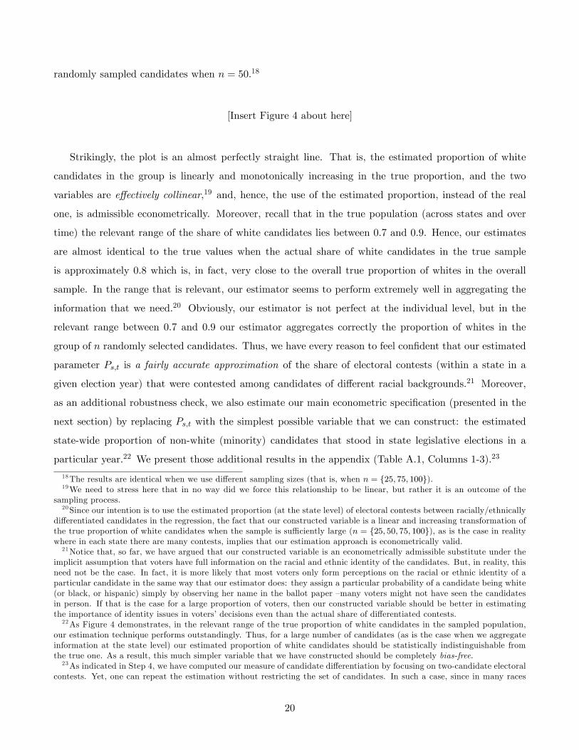
randomly sampled candidates when n = 50.18

[Insert Figure 4 about here]

Strikingly, the plot is an almost perfectly straight line. That is, the estimated proportion of white

candidates in the group is linearly and monotonically increasing in the true proportion, and the two

variables are effectively collinear,19 and, hence, the use of the estimated proportion, instead of the real

one, is admissible econometrically. Moreover, recall that in the true population (across states and over

time) the relevant range of the share of white candidates lies between 0.7 and 0.9. Hence, our estimates

are almost identical to the true values when the actual share of white candidates in the true sample

is approximately 0.8 which is, in fact, very close to the overall true proportion of whites in the overall

sample. In the range that is relevant, our estimator seems to perform extremely well in aggregating the

information that we need.20 Obviously, our estimator is not perfect at the individual level, but in the

relevant range between 0.7 and 0.9 our estimator aggregates correctly the proportion of whites in the

group of n randomly selected candidates. Thus, we have every reason to feel confident that our estimated

parameter Ps,t is a fairly accurate approximation of the share of electoral contests (within a state in a

given election year) that were contested among candidates of different racial backgrounds.21 Moreover,

as an additional robustness check, we also estimate our main econometric specification (presented in the

next section) by replacing Ps,t with the simplest possible variable that we can construct: the estimated

state-wide proportion of non-white (minority) candidates that stood in state legislative elections in a

particular year.22 We present those additional results in the appendix (Table A.1, Columns 1-3).23

18The results are identical when we use different sampling sizes (that is, when n = {25, 75, 100}).19We need to stress here that in no way did we force this relationship to be linear, but rather it is an outcome of the

sampling process.20Since our intention is to use the estimated proportion (at the state level) of electoral contests between racially/ethnically

differentiated candidates in the regression, the fact that our constructed variable is a linear and increasing transformation ofthe true proportion of white candidates when the sample is suffi ciently large (n = {25, 50, 75, 100}), as is the case in realitywhere in each state there are many contests, implies that our estimation approach is econometrically valid.21Notice that, so far, we have argued that our constructed variable is an econometrically admissible substitute under the

implicit assumption that voters have full information on the racial and ethnic identity of the candidates. But, in reality, thisneed not be the case. In fact, it is more likely that most voters only form perceptions on the racial or ethnic identity of aparticular candidate in the same way that our estimator does: they assign a particular probability of a candidate being white(or black, or hispanic) simply by observing her name in the ballot paper —many voters might not have seen the candidatesin person. If that is the case for a large proportion of voters, then our constructed variable should be better in estimatingthe importance of identity issues in voters’decisions even than the actual share of differentiated contests.22As Figure 4 demonstrates, in the relevant range of the true proportion of white candidates in the sampled population,

our estimation technique performs outstandingly. Thus, for a large number of candidates (as is the case when we aggregateinformation at the state level) our estimated proportion of white candidates should be statistically indistinguishable fromthe true one. As a result, this much simpler variable that we have constructed should be completely bias-free.23As indicated in Step 4, we have computed our measure of candidate differentiation by focusing on two-candidate electoral

contests. Yet, one can repeat the estimation without restricting the set of candidates. In such a case, since in many races

20

3.2.2 Main econometric specification

After presenting in detail the method for estimating the share of all state-wide electoral contests for local

legislative offi ces that were contested among candidates of different racial backgrounds, we are now ready

to introduce this variable into our estimation. As stated earlier, the purpose of this exercise is to identify

whether the importance of inequality as a key determinant of redistributive outcomes varies with the

salience of issues related to race, which we proxy by estimating the share of differentiated (heterogeneous)

contests. Naturally, our unit of analysis is now the state-election (not simply calendar) year, which

implies that our sample size is halved since elections for state legislative offi ces take place every two years.

Formally, we estimate the following model:

Ts,t = β0 +τ=∑τ=1

Ts,t−τ + β1Ps,t + β2Ps,t ∗(

yy50

)+ β3

(yy50

)+ β4ERFs,t + β5ERFs,t ∗

(yy50

)s,t

+X′s,tγ +

αs + λt + εs,t (2)

where the focus is on candidate differentiation Ps,t. All other variables in equation (2), including the

controls, are defined as before. Again, in some specifications, we replace the mean to median (pre-tax)

income ratio as our measure of income inequality with the variables presented in earlier sections of the

paper (e.g., skewness). We also estimate a version of the model that includes more interactions between

our key variables, such as the interaction between our inequality measure and the index of ethnic and

racial fragmentation.

3.3 Results

Tables 2 and 3, and Figures 5 through 11 present the main results of, and some variations on, the

estimating equation (2).

[Insert Tables 2 and 3 about here]

more than two candidates can compete for one (or even more than two seats in the case of MMDs), the concept of calculatingthe probability that an electoral race is contested between two candidates of different ethnic or racial backgrounds is a bitproblematic. For this reason, we calculate instead —based on the assigned probability of being non-white 1−wis,t that we haveestimated in Step 3—the state-wide proportion of non-white (minority) candidates that stood in state legislative elections ina particular election year. Figure A.6 (in the appendix) reports the estimates of our basic econometric specification when wereplace Ps,t —the estimated state-wide proportion of differentiated electoral contests—with our new variable detailed above.

21

As we can see from Table 2, the coeffi cient on the interaction term is negative and statistically

significant at the 5% level in all specifications. This implies that as the share of differentiated electoral

contests in a given state is increasing, the positive effect of inequality on redistribution is diminishing. The

result is robust to using alternative measures of inequality in addition to the mean-to-median (pre-tax)

income ratio ( yy50), such as the skewness of the income distribution and the relative mean-to-median (pre-

tax) income difference ( y−y50

y50). Also note that, not surprisingly, the coeffi cient on β1 is positive as minority

candidates are more likely to represent poorer constituencies, given the patterns of income inequality across

different racial and ethnic groups that prevail in the U.S. over the last four decades. Moreover, in addition

to employing different measures of inequality, in Table 3 we also estimate our model of equation (2) using

alternative measures of redistributive outcomes. That is, we use the effective individual and total income

tax rates, and state social transfers as a percent of state GDP as our dependent variables. As it is clear

from all specifications in both tables, the empirical evidence support our conditional hypothesis: The

initially strong effect of income inequality is diminishing in the degree of candidate differentiation.

[Insert Figures 5 to 11 about here]

Yet, interpreting the output in Tables 2 and 3 is not straightforward. In fact, we are interested

in estimating the marginal effects of inequality on redistribution conditioning on the degree of race-

issue salience (proxied by the degree of candidate differentiation and the share of heterogeneous electoral

contests). Therefore, in Figures 5 through 11 we plot the conditional marginal effects of the estimates

presented in Tables 2 and 3 under various alternative specifications. If one pays close attention to all

figures, the pattern that emerges is quite clear: When a small fraction of all state-wide electoral contests

in a given election year are contested among candidates of different racial and ethnic backgrounds, then

inequality (irrespective of how we measure it) has a positive and significant (both economically and

statistically) effect on redistribution, measured as the effective tax rate or social transfers. But when

more than a quarter of all contests are contested between differentiated candidates, then the effect of

inequality on redistribution fails to be statistically significant. That is, when non-economic issues such as

matters related to race are relatively more salient, inequality ceases to be an important determinant of

redistributive outcomes.

[Insert Figure 12 about here]

22

Finally, in Figure 12 we again plot the conditional marginal effects of inequality on redistribution, but

this time we condition on the index of overall racial heterogeneity within a state. The intuition is that

perhaps our constructed variable simply acts as a proxy for racial heterogeneity: It might be the case

that in states with high racial and ethnic heterogeneity most of the electoral contests are fought between

candidates of different racial backgrounds. In fact, a quick look at Figure 2 reveals a significant correlation

between ethnic and racial heterogeneity and the presence of many differentiated electoral contests. As a

result, this conditional effect that we capture might be driven by overall racial heterogeneity. To check

against this claim, in Figure 12, we plot the marginal effects of inequality (the mean-to-median ratio) on

the effective tax rate conditional on racial and ethnic heterogeneity, measured by the ERF index. One

can observe the conditional effect we have estimated before is absent. If anything, as racial heterogeneity

increases, the effect of inequality on redistribution is positive but not statistically significant. This, in

turn, implies that if the positive effect that we have estimated in Figures 5 to 11 is biased, then this

bias works against our hypothesis. That is, perhaps we are underestimating the true positive effect of

inequality on redistribution.

4 Discussion

4.1 Relationship with the literature

Before discussing the empirical and policy implications of our findings, we first would like to comment

on how those findings align with previous literature. First, we should note that certainly we are not

the first to argue that one can recover the predicted Meltzer and Richard (1981) effect of inequality on

redistributive outcomes. Previous studies by Karabarbounis (2011) and Lupu and Pontusson (2011) have

shown that the relative incomes of poor, middle class, and rich voters might matter in determining redis-

tributive outcomes. In that respect, including different and multiple moments of the income distribution

that can capture those relative changes (e.g., the y90/y and the y10/y ratios, as in Karabarbounis 2011, or

the skewness of the income distribution, as in Lupu and Pontusson 2011) might be able to reconcile the

theoretical predictions with empirical regularities. Yet, in our analysis we have taken those considerations

into account when building our econometric model. It turns out that: a) our results do not hinge on

those relative changes in inequality between different income groups, and b) introducing a second dimen-

sion in our analysis —the salience of non-economic matters, captured by the fraction of heterogeneous

electoral contests between differentiated candidates—is necessary in order to empirically recover the the-

23

oretically predicted effect of inequality on redistribution. Simply put, adding those additional moments

of the income distribution into the regression was not suffi cient to generate a positive and statistically

significant effect of inequality on redistribution. We attribute this difference to the following two reasons.

First, our study focuses exclusively on the U.S. and exploits within-country variation, thus keeping fixed

other determinants (e.g., institutions or culture) of redistributive outcomes. In contrast, both studies by

Karabarbounis (2011) and Lupu and Pontusson (2011) use cross-country data. That is, their findings are

relevant for a group of OECD countries and might not carry over in the case of the U.S.24 Second, unlike

Lupu and Pontusson (2011), we measure income inequality using gross (before deductions and taxes)

earnings. As a result, we can capture changes in the distribution of income (and inequality) before any

distortions being introduced due to redistributive taxation and transfers.

Our paper is also related to another strand in the literature that links preferences and demand for

redistribution to ethnic and racial heterogeneity (e.g., Alesina et al. 1999, 2016; Alesina and Glaeser 2004;

Dahlberg et al. 2012; Snyder and Testa 2016). Our results do not contradict those findings. In fact, our

results in Table 1 support the hypothesis that more ethnic or racial heterogeneity is related with lower

levels of redistribution. We complement these studies by adding a new dimension: The salience of issues

related to ethnic or racial identity. That is, we find that irrespective of the arguably important effect that

voter ethnic and racial heterogeneity has on the demand for redistribution, when issues related to race

or ethnicity become salient, inequality ceases to be the most predominant determinant of redistributive

outcomes, and vice versa. Thus, our results add to the findings of the literature on the relationship

between ethnic heterogeneity and redistribution by stressing the importance of not only voter, but also

candidate, heterogeneity.

4.2 Implications and final remarks

Despite the fact that our findings contribute to the discussion of the relationship between ethnic hetero-

geneity and redistribution, our study, of course, has certain limitations. First, one should apply caution in

interpreting our findings as causal, as inequality itself can be an outcome of redistributive policies (or lack

thereof). If redistributive policies have long-lasting outcomes, then the distribution of income today can

depend on redistributive policies of the past which, in turn, might be correlated with current redistributive

policies, thus giving rise to worries about reverse causality. We have tried to deal with such complications

in two ways. As noted above, we have used gross (pre-deductions and taxes) earnings in order to calculate

24One plausible explanation is that issues of race and ethnic diversity are more pronounced in the U.S. context.

24

income inequality. Moreover, we have used a lagged dependent variable in our estimation to account for

the possibility that current redistributive policies are correlated with past ones.

In addition and, perhaps, more importantly inequality and ethnic or racial heterogeneity might be

correlated. In other words, it can be the case that in ethnically or racially more diverse communities

income inequality is larger. That is, ethnic or racial heterogeneity might simply be a proxy for ethnic

income inequality (Alesina et al. 2016). This, in turn, implies that if inequality is higher in relatively

more racially heterogeneous communities —perhaps because minorities are relatively poorer— then we

should expect to see more minority candidates, and, hence, more differentiated electoral contests in more

unequal communities. Nevertheless, this does not negate the main point that this paper makes: Candidate

heterogeneity is an equally important determinant of redistributive outcomes. Regardless of whether

or not candidate differentiation is a proxy for ethnic inequality and its direct effect on redistributive

outcomes, our estimates show that when the salience of issues related to identity is high (e.g., the percent

of heterogenous electoral contests is high), then redistributive outcomes do not seem to be sensitive to

changes in income inequality.

In the appendix, we address in more detail some issues related to candidate selection which could be

endogenous to the relationship between inequality (especially between different ethnic and racial groups)

and redistribution (or the absence of it). What the evidence reveals is that, in our context, there is little

reason to worry excessively about such issues of endogeneity: candidate selection appears to be orthogonal

to income inequality and redistribution, even if one allows for a non-linear relationship (see Figure 13).25

In fact, if anything, candidate (ethnic and racial) differentiation seems to be correlated with overall ethnic

and racial heterogeneity of the population (see Figure 2); but the latter, as shown above (Figure 12), has a

starkly different marginal effect on the inequality-redistribution nexus, in contrast to the effect of interest

that we have estimated for candidate differentiation.

[Insert Figure 13 about here]

Of course, there is still much to be done in order for all the aspects of the underlying mechanism to

come to the surface. Indeed, it may be that when two candidates of different ethnic or racial background25We have regressed Ps,t (the state-wide percent of electoral contests between candidates of different racial and ethnic

backgrounds) on income inequality and redistribution using the same controls as in equation (2), as well as state- andyear-specific fixed effects. In Figure 13, we plot the estimates of this regression: the partial regression plot (also known asthe adjusted partial residual plot) and the augmented component-plus-residual plot (also known as the augmented partialresidual plot) which is better suited for detecting any nonlinearities in the data. There appears to be no correlation betweencandidate differentiation and inequality.

25

compete they do not have to pander to the economic median (and her preference for more redistribution),

and, thus, they do not promise any redistribution as they can secure enough votes by playing the identity

card. However, it also may be that parties or interest groups select minority candidates in constituencies

with high levels of income inequality —which might also be more diverse— in order to divert attention

from issues of class to those of identity. Regardless of the exact mechanism taking place, the fact of

the matter is that candidate heterogeneity appears to be an important determinant of redistributive

outcomes that counteracts income inequality: As candidate heterogeneity increases, the median voter in

the economic dimension is no longer decisive since the non-economic dimension becomes an increasingly

relevant determinant of voting decisions.26 This paper is the first to our knowledge that documents

this effect by compiling a large volume of electoral contests at the state level for a long period of time.

Exploring this relationship and the exact mechanisms taking place in more detail is something that future

research should focus on.

The implications of our findings are twofold. On the one hand, they highlight that in the context of

multi-dimensional electoral competition, the relative salience of non-economic matters might have impor-

tant spill-over effects on redistributive outcomes. This, in turn, implies that factors and mechanisms that

affect issue salience might be important determinants of redistributive policies and outcomes. Therefore,

our work highlights the importance of exploring how issue salience arises endogenously.

On the other hand, our findings also point to a relationship between polarization on non-economic

matters and inequality. In our analysis, we chose to focus on issues related to racial and ethnic identity

—which seem to matter in the context of U.S. politics. Yet, issues of ethnic identity are not the only ones

which are salient; in recent years, for example, religion, and social ideology (e.g., issues such as abortion

or same-sex marriage) have become equally important as race and ethnicity in the context of U.S. and

world politics. Future work should explore the role of candidate heterogeneity in a variety of other

dimensions, not exclusively race and ethnicity. In fact, social polarization at the candidate level might

prove to be one of the most predominant determinants of redistributive outcomes as it has the potential

of rasing the salience of non-economic matters, thus surfacing the conflict between class and identity

politics (Mukand and Rodrik 2016). While the relationship between inequality, social polarization, and

redistributive policies is certainly worth exploring in greater detail, we defer it to future research.

Finally, our work also connects to the literature on the determinants of liberal democracy (Mukand

26This finding is in the spirit of previous theoretical findings (e.g., Krasa and Polborn 2014; Matakos and Xefteris 2016) thatdocument strong spill-over effects from non-economic dimensions to economic ones in the framework of multi-dimensionalelectoral competition.

26

and Rodrik 2015) and the prevalence of ethnic cleavages and in some cases conflict in environments where

inequality is prevalent (Esteban and Ray 2008). Our work uncovers a conflict between the politics of

class and identity, and, hence, can provide a rationale behind the prevalence and the increased salience

of identity cleavages (e.g., race, religion, ethnicity, or culture) in countries where income (and perhaps

ethnic) inequality are heightened. Since in those societies, political competition most likely revolves

around identity cleavages rather than class cleavages, it can be the case that they are less conducive to

liberal —used in the traditional sense—politics (Mukand and Rodrik 2015), thus jeopardizing further the

role of ethnic, religious, or racial minorities in the political process.

References

[1] Ahler, D.J., J. Citrin, M.C. Dougal, and G.S. Lenz (2015). “Can Your Face Win You Votes? Exper-

imental Tests of Candidate Appearance’s Influence on Electoral Choice,”mimeo

[2] Alesina, A., and D. Rodrik (1994). “Distributive Politics and Economic Growth,”Quarterly Journal

of Economics, 109 (2): pp. 465-490.

[3] Alesina, A., R. Baqir, and W. Easterly (1999). “Public Goods and Ethnic Divisions,” Quarterly

Journal of Economics, 114 (4): pp. 1243-1284.

[4] Alesina, A., E.L. Glaeser, and B. Sacerdote (2001). “Why Doesn’t the United States Have a European-

Style Welfare State?”Brookings Papers on Economic Activity, 2: pp. 187-254.

[5] Alesina, A., and E. La Ferrara (2002). “Who Trusts Others?”Journal of Public Economics, 85 (1-2):

pp. 207-234.

[6] Alesina, A., and E.L. Glaeser (2004). Fighting Poverty in the US and Europe: A World of Difference,

Oxford: Oxford University Press.

[7] Alesina, A., and P. Giuliano (2010). “Preferences for Redistribution”, in Handbook of Social Eco-

nomics (J. Benhabib, M.O. Jackson and A. Bisin eds.), vol. 1A, The Netherlands: North Holland,

pp. 93-131.

[8] Alesina, A., S. Michalopoulos, and E. Papaioannou (2016). “Ethnic Inequality,”Journal of Political

Economy, 124 (2): pp. 428-488.

[9] Atkinson, A.B., T. Piketty, and E. Saez (2011). “Top Incomes in the Long Run of History,”Journal

of Economic Literature, 49 (1): pp. 3-71.

27

[10] Besley, T., and I. Preston (2007). “Electoral Bias and Policy Choice: Theory and Evidence,”Quar-

terly Journal of Economics, 122 (4): pp. 1473-1510.

[11] Boudreau, C., C.S. Elmendorf, and S.A. MacKenzie (2014). “Racial or Spatial Voting? The Effects

of Candidate Ethnicity and Ethnic Group Endorsements in Low-Information Elections,”mimeo

[12] Bouton, L., P. Conconi, F. Pino, and M. Zanardi (2014). “Guns and Votes,”NBER Working Paper

20253.

[13] Bursztyn, L., M. Callen, B. Ferman, S. Gulzar, A. Hasanain, and N. Yuchtman (2016). “Identifying

Ideology: Experimental Evidence on Anti-Americanism in Pakistan,”mimeo

[14] Campante, F.R. (2011). “Redistribution in a Model of Voting and Campaign Contributions,”Journal

of Public Economics, 95 (5-6): pp. 646-656.

[15] Citrin, J., D.P. Green, and D.O. Sears (1990). “White Reactions to Black Candidates: When does

Race Matter?”Public Opinion Quarterly, 54: pp. 74-96.

[16] Dahlberg, M., K. Edmark, and H. Lundqvist (2012). “Ethnic Diversity and Preferences for Redistri-

bution,”Journal of Political Economy, 120 (1): pp. 41-76.

[17] Downs, A. (1957). An Economic Theory of Democracy. Harper and Row: New York, USA.

[18] Esteban, J., and D. Ray (2008). “On the Salience of Ethnic Conflict,”American Economic Review,

98 (5): pp. 2185-2202.

[19] Iversen, T., and D. Soskice (2006). “Electoral Institutions and the Politics of Coalitions: Why Some

Democracies Redistribute More Than Others,”American Political Science Review, 100 (2): pp. 165-

181.

[20] Karabarbounis, L. (2011). “One Dollar, One Vote,”Economic Journal, 121 (3): pp. 621-651.

[21] Klarner, C., W.D. Berry, T. Carsey, M. Jewell, R. Niemi, L. Powell, and J.M. Snyder (2013). State

Legislative Election Returns (1967-2010): ICPSR34297-v1. Ann Arbor, MI: Inter-university Consor-

tium for Political and Social Research. DOI: http://doi.org/10.3886/ICPSR34297.v1

[22] Krasa, S., and M. Polborn (2010). “The binary policy model,”Journal of Economic Theory, 145 (2):

pp. 661-688.

[23] Krasa, S., and M. Polborn (2012). “Political Competition between Differentiated Candidates,”Games

and Economic Behavior, 76 (1): pp. 249-71.

28

[24] Krasa, S., and M. Polborn (2014). “Social Ideology and Taxes in a Differentiated Candidates Frame-

work,”American Economic Review, 104(1): pp. 308-322.

[25] Lind, J. (2007). “Fractionalization and the Size of Government,” Journal of Public Economics, 91

(1-2): pp. 51-76.

[26] Lindbeck, A., and J. Weibull (1987). “Balanced-budget Redistribution as the Outcome of Political

Competition,”Public Choice, 52 (2): pp. 273-297.

[27] Lupu, N., and J. Pontusson (2011). “The Structure of Inequality and the Politics of Redistribution,”

American Political Science Review, 105 (2): pp. 316-336.

[28] Matakos, K., and D. Xefteris (2016). “Divide and Rule: Redistribution in a Model with Differentiated

Candidates,”forthcoming in Economic Theory

[29] McCarty, N., K.T. Poole, and H. Rosenthal (2006). Polarized America: The Dance of Ideology and

Unequal Riches. Cambridge, MA: MIT Press.

[30] McKelvey, R.D., and R.E. Wendell (1976). “Voting Equilibria in Multidimensional Choice Spaces,”

Mathematics of Operations Research, 1: pp. 144-158.

[31] Meltzer, A.H., and S.F. Richard (1981). “A Rational Theory of the Size of Government,”Journal of

Political Economy, 89 (5): pp. 914-27.

[32] Mukand, S.W., and D. Rodrik (2015). “The Political Economy of Liberal Democracy,”mimeo.

[33] Mukand, S.W., and D. Rodrik (2016). “Ideas versus Interests: A Unified Political Economy Frame-

work,”mimeo.

[34] Padró i Miquel, G. (2007). “The Control of Politicians in Divided Societies: The Politics of Fear,”

The Review of Economic Studies, 74 (4): pp. 1259-74.

[35] Pecoraro, B. (2014). “Inequality in Democracies: Testing the Classic Democratic Theory of Redis-

tribution,”Economics Letters, 123: pp. 398-401.

[36] Persson, T., and G. Tabellini (1994). “Is Inequality Harmful for Growth? Theory and Evidence,”

American Economic Review, 84 (3): pp. 600-621.

[37] Persson, T., and G. Tabellini (2003). The Economic Effects of Constitutions. Cambridge, MA: MIT

Press.

29

[38] Piketty, T., and E. Saez (2003). “Income Inequality in the United States, 1913-1998,” Quarterly

Journal of Economics, 118 (1): pp. 1-39.

[39] Plott, C.R. (1967). “ A notion of Equilibrium and its Possibility Under Majority Rule,”American

Economic Review, 57 (5): pp. 787-806.

[40] Polborn, M., and J.M. Snyder (2016). “Party Polarization in Legislatures with Offi ce-Motivated

Candidates,”mimeo

[41] Prato, C. (2016). “Electoral Competition and Policy Feedback Effects,”mimeo.

[42] Rodriguez, F.C. (1999). “Does Distributional Skewness Lead to Redistribution? Evidence from the

United States,”Economics and Politics, 11 (2): pp. 171-199.

[43] Roemer, J.E. (1998). “Why the Poor Do Not Expropriate the Rich: An Old Argument in New Grab.”

Journal of Public Economics, 70 (3): pp. 399-424.

[44] Roemer, J.E. (2005). “Will Democracy Engender Equality?”Economic Theory, 25 (1): pp. 217-234.

[45] Rosenstone, S., and J.-M. Hansen (1993). Mobilization, Participation and Democracy in America.

New York: MacMillan.

[46] Snyder, J.M., and C. Testa (2016). “The Value of Voting Rights: Black Elected Offi cials and Public

Spending in the US South,”mimeo

[47] Sparks, D.B., and C.S. Watts (2010). “Race Still Matters: Racial Attitudes and Their Effects on

Candidate Evaluations,”mimeo

30

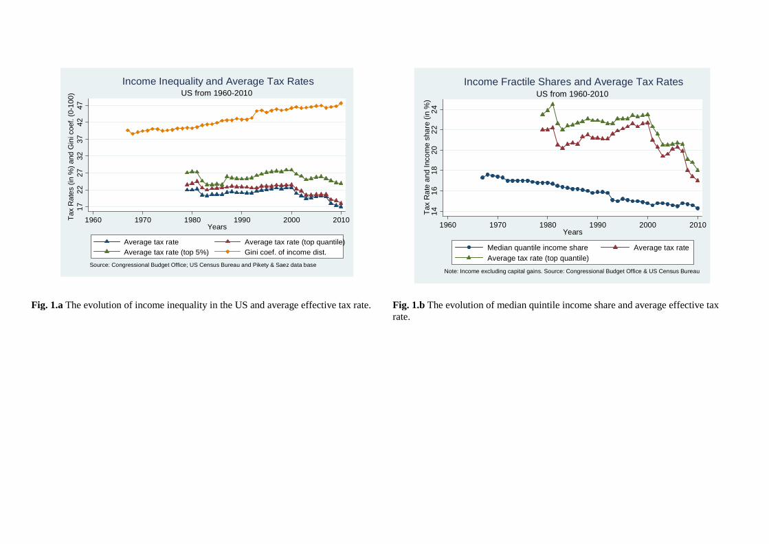
Fig. 1.a The evolution of income inequality in the US and average effective tax rate. Fig. 1.b The evolution of median quintile income share and average effective tax

rate.

1722

2732

3742

47T

ax R

ates

(in

%)

and

Gin

i coe

f. (0

-100

)

1960 1970 1980 1990 2000 2010Years

Average tax rate Average tax rate (top quantile)Average tax rate (top 5%) Gini coef. of income dist.

Source: Congressional Budget Office; US Census Bureau and Pikety & Saez data base

US from 1960-2010Income Inequality and Average Tax Rates

141

618

202

224

Tax

Rat

e an

d In

com

e sh

are

(in %

)

1960 1970 1980 1990 2000 2010Years

Median quantile income share Average tax rateAverage tax rate (top quantile)

Note: Income excluding capital gains. Source: Congressional Budget Office & US Census Bureau

US from 1960-2010Income Fractile Shares and Average Tax Rates

Fig. 2.a Income inequality (measured by the mean-to-median ratio) across US States from 1979 to 2012: averages (left) and changes over time (right)

Fig. 2.b Effective income tax rate across US States from 1979 to 2012: averages (left) and changes over time (right)

Fig. 2.c Ethnic/racial heterogeneity (measured by the ERF index) across US States from 1979 to 2012: averages (left) and changes over time (right)

Fig. 3. Candidate racial/ethnic heterogeneity (measured by the percent of state-wide electoral contestes between candidates of different race) across US States from 1979 to 2012: averages (left) and changes over time (right)

Fig. 4 Estimated and true proportion of white population in randomly selected groups of 50 candidates (Note: dashed line represents the 45-degree line; red lines represent the 95% confidence intervals).

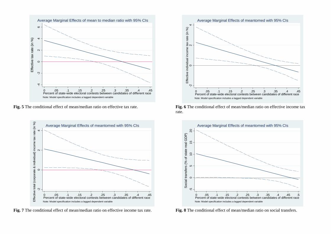
Fig. 5 The conditional effect of mean/median ratio on effective tax rate. Fig. 6 The conditional effect of mean/median ratio on effective income tax

rate.

Fig. 7 The conditional effect of mean/median ratio on effective income tax rate. Fig. 8 The conditional effect of mean/median ratio on social transfers.

-4-2

02

46

Effe

ctiv

e ta

x ra

te (

in %

)

0 .05 .1 .15 .2 .25 .3 .35 .4 .45Percent of state-wide electoral contests between candidates of different raceNote: Model specification includes a lagged dependent variable

Average Marginal Effects of mean to median ratio with 95% CIs

-20

24

Effe

ctiv

e in

divi

dual

inco

me

tax

rate

(in

%)

0 .05 .1 .15 .2 .25 .3 .35 .4 .45Percent of state-wide electoral contests between candidates of different raceNote: Model specification includes a lagged dependent variable

Average Marginal Effects of meantomed with 95% CIs

-20

24

Effe

ctiv

e to

tal (

corp

orat

e &

indi

vidua

l) in

com

e ta

x ra

te (

in %

)

0 .05 .1 .15 .2 .25 .3 .35 .4 .45Percent of state-wide electoral contests between candidates of different raceNote: Model specification includes a lagged dependent variable

Average Marginal Effects of meantomed with 95% CIs

-50

510

1520

Soc

ial t

rans

fers

(%

of s

tate

rea

l GD

P)

0 .05 .1 .15 .2 .25 .3 .35 .4 .45 .5Percent of state-wide electoral contests between candidates of different raceNote: Model specification includes a lagged dependent variable

Average Marginal Effects of meantomed with 95% CIs

Fig. 9 The conditional effect of relative difference of mean to median income on the effective tax rate.

Fig. 10 The conditional effect of the skewness of the income distribution on state social transfers.

Fig. 11 The conditional effect of the skewness of the income distribution on the effective tax rate.

Fig. 12 The conditional effect of mean/median ratio on the effective tax rate.

-50

510

Effe

ctiv

e ta

x ra

te (

in %

)

0 .05 .1 .15 .2 .25 .3 .35 .4 .45Percent of state-wide electoral contests between candidates of different raceNote: Model specification includes a lagged dependent variable; Inequality measured as the relative mean-median difference

Average Marginal Effects of rmeanmeddif with 95% CIs

-1-.

50

.51

1.5

Soc

ial t

rans

fers

(%

of

stat

e G

DP

)

0 .05 .1 .15 .2 .25 .3 .35 .4 .45

Percent of state-wide electoral contests between candidates of different raceNote: Model specification includes a lagged dependent variable

Average Marginal Effects of skewness with 95% CIs

-20

24

6E

ffect

ive

tax

rate

(in

%)

0 .05 .1 .15 .2 .25 .3 .35 .4 .45Percent of state-wide electoral contests between candidates of different race

Average Marginal Effects of skewness with 95% CIs

-50

510

Effe

ctiv

e ta

x ra

te (

in %

)

1 1.25 1.5 1.75 2 2.25 2.5 2.75 3Racial heterogeneity

Note: Model specification includes a lagged dependent variable

Average Marginal Effects of meantomed with 95% CIs

Fig. 13 The correlation between income inequality (measured by the mean-to-median ratio) and candidate heterogeneity (measured by the percent of state-wide electoral contests between candidates of different race): augmented component-plus-residual plot (left) and adjusted partial residual plot (right).

WA IA

HI

WY

WA

AK

OHVT

AKMA

CT

VT

OR

PA

MI

INOH

MI

ORME

HI

WAMIOR

WV

WA

OK

AK

PA

CACTKS

PA

WA

ME

NV

CT

IN

KS

KS

WY

WIIL

OK

OKNY

NVMEWI

UT

UT

CT

MNNE

ME

IAID

WA

WV

ID

IN

NV

MN

IN

VTILILNHOH

OH

SD

PA

MI

WINEMA

CAWI

AZ

OHWV

WYIL

OR

MO

VT

AK

SD

WI

VT

NE

MN

MT

COCO

NYOHIAIA

IL

WIOR

UT

MA

CA

MT

NH

RI

MTNY

OKND

UTVTIA

CA

MEMN

KS

PA

SDNJ

ID

IA

ME

RI

ME

CO

MNWINVCT

DE

MN

NY

IA

WIND

KY

MO

WI

HI

INNHAKWYRINDDEND

MNNHMEMINH

WY

NH

WV

HI

MT

KY

NV

HI

VT

NCSC

WA

VA

RI

TNIA

AK

WI

SC

MT

NVHI

OR

OR

MOMA

SCVT

NCSCMT

ND

CTDEMNSCMTMO

DE

IA

HI

MA

RI

AZ

MA

ID

WY

AKNM

NM

ND

PA

MOSD

WY

AR

NV

SDMO

OR

NJ

IA

KYMOMA

TN

IA

IN

ND

FLSD

GA

VAOHDE

SD

TN

NE

VAMNOHAK

AR

AZ

WY

MESD

IA

SCKY

CT

DENY

AK

VT

MI

AK

WVME

MN

CO

WA

NV

MN

AZ

SC

WY

WI

WI

WIMI

MNWV

ME

SDUT

NHSD

SD

ID

SCINNC

IA

CT

FL

NH

ND

IDNE

TN

VA

ND

COWIARWANC

WY

VT

DE

WVGAKSMO

DE

ID

AR

CA

SC

MO

CO

NC

MT

ID

AK

IA

DE

NH

CO

CO

OH

SD

IL

NY

SD

NE

NDRI

AZ

DE

IDMTAKPA

OH

HI

NYMT

PAMT

KSCT

OH

PACT

SD

ME

IN

NHMIWACT

TXAR

SC

FLSCID

NE

DE

NE

ILFL

OHMO

ME

NCOR

WAGAMONDKS

PAMIVACOWY

INMA

WY

RI

IN

TX

NHINAKPA

KYTX

MN

MO

HI

UTNE

ND

ND

IN

HIMT

SD

ORILID

AZRIKS

TN

OR

NC

KYTN

OK

WY

OKIN

GAVA

WA

NE

NDAZ

KYOR

OH

WVSC

KY

MA

TN

KYRI

AR

MT

WA

OK

UT

NH

INCT

NV

MNOKME

AK

WA

MIWV

IA

OK

WV

FL

KYCO

OH

GAMN

CO

AR

SC

DE

ID

NE

MO

RI

RIVTMIFLUT

WANM

ND

KYNV

CAGA

AR

KY

HI

TN

MI

DE

VANY

GAKS

NH

HI

OK

IDGA

DE

ARNE

WI

AZ

MT

MA

WY

VAME

TXNJ

PA

CT

NM

GA

GA

KY

KS

MA

NC

MTOK

NH

FL

HINV

GA

VTAR

MO

GAOKUT

VA

NE

NMPA

NH

NV

HI

MA

ARILNC

PATNDE

RI

NETN

UT

AK

NV

TX

IL

MA

CA

CAID

ID

NE

CO

RI

NM

SC

SC

OKTX

KS

IL

OR

CT

UT

ORCO

RINMNCWV

IL

AR

OKVAWV

NM

CO

HI

AZ

MA

UT

WVWY

KY

IN

MA

NY

MI

NCVA

NC

NM

AZ

UT

NMNC

AR

AZ

PANMFL

FL

OH

TX

MIAR

GA

CT

KS

NV

UT

KS

FL

RI

NC

MO

NM

GA

AZ

MI

OK

KY

ARNY

AZ

CO

NY

IL

TN

NC

CA

NV

IL

NY

TNCA

GA

CAUTKSTX

NY

NY

WV

FL

TN

TX

VAORTN

VAFL

KSVA

CA

TX

NM

VACA

IL

FLTN

AZ

NM

NYWVTX

TX

FLTX

TX

CATXFLCA

NM

AZ

1.9

1.9

52

2.0

52.

1

1.1 1.15 1.2 1.25 1.3Mean-to-median ratio

Note: Regression model includes state, year fixed effects and a lagged dependent variable; standard errors are clustered at the state level

Lowess smooth (green line) bandwith = 0.8

Dep. var.: Percent of state-wide contests between candidates of different race

Augmented component-plus-residual plot

WY

IL

VT

SCMOWY

AZWV

ND

HI

MA

WA

WY

MI

OKTN

WVMO

CA

SC

SC

OH

NY

DE

PA

SD

MO

SD

TN

COAR

UT

KSWI

MTKS

MEME

AZ

ORKS

WV

OR

VTME

SC

DEWI

IN

DEOK

UT

MICA

ND

HI

IA

WVNHNE

WAWY

AK

MI

OK

FLAK

IL

SDDE

NM

HI

MA

MINC

NE

GA

OK

GA

HI

CO

AK

OHCT

IN

NM

WA

TXPA

AR

NH

CONH

NVDE

MN

ND

KSMO

NHKY

FL

GA

CTWINC

TNUT

TN

WY

ORGAIDAZ

NM

NY

NYNEMOTX

WA

MT

NMOH

NMFL

PA

KY

MNIDFL

NVOH

INPA

ND

MEMN

RINY

HI

WI

MAMNME

OR

UTMNCA

WVAK

NV

AZ

OR

WY

IA

OK

CO

MAIANMORTN

ND

SC

SD

CA

HI

MI

MT

AR

HI

TXKY

OKNEVT

AZ

RIIL

KY

DE

RI

ID

IL

SD

KY

NY

TX

ARNV

IANC

HI

IN

AK

CAVT

COWV

HI

NV

NY

CT

MN

OK

OR

NE

MAIA

CO

MT

AK

NE

TX

AZ

CA

NV

DE

TN

VA

WV

NHFLUTKS

MOCT

MTCTFLNCNJ

UT

GA

WV

COND

PAMAVT

CO

ID

UT

AZ

GANHTXIA

CTAK

PA

IATN

PAIL

MIID

OR

ID

NV

MA

IN

ND

NCOH

TXNC

NC

SD

KS

ILVAKYPACTWA

IL

FLWI

MOIA

SDME

DE

NV

WA

WAGA

IAAK

WI

ME

IN

NMSD

KY

IL

NY

WI

NV

ID

OK

AZ

VTUT

NC

RI

CT

ND

IN

NE

NV

WA

RI

OR

KSMI

UT

WI

NM

NE

RI

WV

NJ

SCNYIN

SC

CT

MO

VT

ID

VAVAVAVAVAVAVAVAVAVAVA

TX

KY

KY

CT

OK

DE

AR

ND

DE

PA

KSRINV

ID

RI

CA

AR

WA

OH

GA

AR

AKCANYGA

RIMA

RIAZSD

FL

INID

FL

AR

WV

IL

ILDE

MNOHGANM

RI

AR

MN

MT

SC

MEMIMTNHOHCTORIN

ID

COAZ

TXILOHTX

OK

MI

AK

OH

MN

CA

IA

NC

MTKYAR

NHWIMNKS

CAOH

NH

VA

SC

WY

VTTN

AR

ORMT

MNKS

IN

RINYWINCMI

MTWA

OH

GA

MTIATX

WY

RI

FL

CO

NCWY

IAVA

NV

NEWV

MT

SD

VT

NE

FLWI

NEMA

NJ

COMI

NM

AK

WYNHMAMEMT

AZ

MI

MA

KYOHKS

MEUTIDMO

NEOHMECA

NY

WV

NMPA

IN

UT

RI

FL

IL

NC

WY

ND

WASD

TX

SC

NE

MTMO

PA

FL

TNAR

NH

SD

KY

CA

UT

CTAR

GA

RI

DE

TNMN

WY

VTPANDCTKY

NC

TX

AK

SC

TN

NCNHAR

PA

MENHMNGAWA

SD

WA

KS

WI

ID

WI

TN

NM

ID

CT

MA

NM

SC

NYMN

NYINNH

WI

MTCANH

UT

AZ

IDARMOMA

IN

TX

KSWY

KY

NY

ND

KY

COIL

IA

HI

MO

NCWA

SC

MA

OR

ND

GA

AK

TN

AZ

MO

ME

HI

TN

CO

TX

IAOR

FL

OK

NE

MEDE

TN

CAMN

PA

HI

MA

OK

CO

NVINOR

ND

KSMI

IL

AZ

NM

NE

IAWVAK

CAHI

FLNV

NM

OK

NVOKMOMEUTSDOKMIND

CO

SC

WI

UT

CT

HIPA

AK

NY

VT

HI

MIKS

GA

VTWA

MO

DEIL

SDSCOH

AZ

WYOR

WV

WV

WY

DE

-.1

-.05

0.0

5.1

e(Y

| X

)

-.05 0 .05 .1e(Mean-to-median ratio | X)

Note: Regression model includes state, year fixed effects and a lagged dependent variable; standard errors are clustered at the state level

coef = .06398621, (robust) se = .05882189, t = 1.09

Dep. var.: Percent of state-wide contests between candidates of different race

Partial regression (Adjusted partial residual) plot

Table 1: The Effect of Inequality on Redistribution (effective tax rate)

Dependent variable

(1)

(2)

(3)

Effective

(4)

tax rate

(5)

(6)

(7)

(8)

(9)

Mean/Median 0.474 0.196 0.918 0.381 0.296

(1.120) (0.557) (1.367) (0.688) (0.612)

Skewness 0.001 0.428 0.122 0.086

(0.065) (0.303) (0.158) (0.128)

P90 / P10 ratio 0.013 0.066 0.018

(0.015) (0.048) (0.018)

P90 / P50 ratio 0.334 (0.543)

P50 / P10 ratio 0.045 (0.144)

Racial heterogeneity -0.852 (0.411)**

-0.247 (0.146)*

-0.754 (0.382)*

-0.232 (0.155)

-0.247 (0.138)*

-0.694 (0.361)*

-0.213 (0.133)

-0.223 (0.145)

-0.765 (0.399)*

GOP control -0.376 -0.174 -0.368 -0.174 -0.175 -0.370 (0.164)** (0.077)** (0.162)** (0.077)** (0.078)** (0.163)**

Other controls

NO

NO

YES

YES

NO

YES

YES

YES

YES

State and Year FE YES YES YES YES YES YES YES YES YES

Lagged dep. NO YES NO YES YES NO YES YES YES

variable

R2 0.75 0.87 0.76 0.87 0.87 0.76 0.87 0.87 0.76

N 1,650 1,600 1,616 1,568 1,600 1,616 1,568 1,568 1,616

* p<0.1; ** p<0.05; *** p<0.01 Note: Robust standard errors clustered at the state level reported in parentheses. Dependent variable is the effective state tax rate (in %). Other controls include: log of real (state) GDP per capita, unemployment rate, female labor force participation rate, growth rate, and a dummy variable indicating whether both chambers of the state's legislature (State House and State Senate) are controlled by a single party.

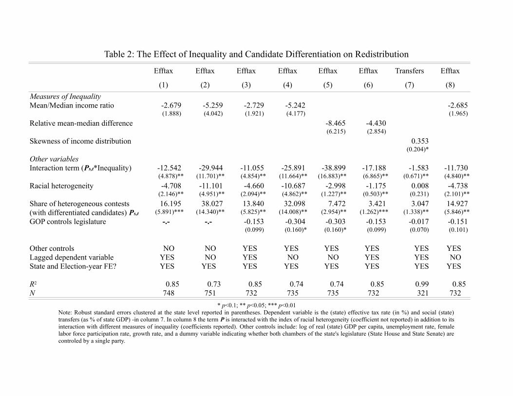
Table 2: The Effect of Inequality and Candidate Differentiation on Redistribution

Efftax

(1)

Efftax

(2)

Efftax

(3)

Efftax

(4)

Efftax

(5)

Efftax

(6)

Transfers

(7)

Efftax

(8)

Measures of InequalityMean/Median income ratio -2.679 -5.259 -2.729 -5.242 -2.685

(1.888) (4.042) (1.921) (4.177) (1.965)

Relative mean-median difference -8.465 -4.430(6.215) (2.854)

Skewness of income distribution 0.353(0.204)*

Other variables Interaction term (Ps,t*Inequality) -12.542 -29.944 -11.055 -25.891 -38.899 -17.188 -1.583 -11.730

(4.878)** (11.701)** (4.854)** (11.664)** (16.883)** (6.865)** (0.671)** (4.840)**

Racial heterogeneity -4.708 -11.101 -4.660 -10.687 -2.998 -1.175 0.008 -4.738(2.146)** (4.951)** (2.094)** (4.862)** (1.227)** (0.503)** (0.231) (2.101)**

Share of heterogeneous contests 16.195 38.027 13.840 32.098 7.472 3.421 3.047 14.927(with differentiated candidates) Ps,t (5.891)*** (14.340)** (5.825)** (14.008)** (2.954)** (1.262)*** (1.338)** (5.846)**

GOP controls legislature -.- -.- -0.153 -0.304 -0.303 -0.153 -0.017 -0.151(0.099) (0.160)* (0.160)* (0.099) (0.070) (0.101)

Other controls NO NO YES YES YES YES YES YESLagged dependent variable YES NO YES NO NO YES YES NOState and Election-year FE? YES YES YES YES YES YES YES YES

R2 0.85 0.73 0.85 0.74 0.74 0.85 0.99 0.85N 748 751 732 735 735 732 321 732

* p<0.1; ** p<0.05; *** p<0.01Note: Robust standard errors clustered at the state level reported in parentheses. Dependent variable is the (state) effective tax rate (in %) and social (state)transfers (as % of state GDP) -in column 7. In column 8 the term P is interacted with the index of racial heterogeneity (coefficient not reported) in addition to itsinteraction with different measures of inequality (coefficients reported). Other controls include: log of real (state) GDP per capita, unemployment rate, femalelabor force participation rate, growth rate, and a dummy variable indicating whether both chambers of the state's legislature (State House and State Senate) arecontroled by a single party.

Table 3: The Effect of Inequality and Candidate Differentiation on Redistribution and Social Spending

Dependent variable

Effective income tax rate State social transfers

Personal Personal Total (as % of state GDP)

(1) (2) (3) (4) (5) (6) (7)

Measures of InequalityMean/Median income ratio -1.256 -1.359 -1.309 -5.759 -6.346

(3.069) (0.813) (1.268) (4.075) (4.009)

Skewness -0.591 -1.628(0.330)* (1.509)

Other variablesInteraction term (Ps,t*Inequality) -7.927 -6.492 -5.636 -21.549 -22.076 -3.048 -6.477

(6.853) (2.327)*** (3.170)* (11.616)* (11.831)* (1.050)*** (3.326)*

Racial heterogeneity -3.844 -2.568 -2.458 -8.159 -8.806 -1.216 -4.157(2.957) (0.928)*** (1.386)* (4.822)* (4.734)* (0.611)* (1.773)**

Share of heterogeneous contests 9.661 7.791 6.548 26.309 27.450 5.342 12.180(with differentiated candidates) Ps,t (8.538) (2.811)*** (4.017) (14.307)* (14.491)* (1.983)*** (5.961)**

Lagged dependent variable NO YES YES YES YES YES NOOther controls YES YES YES YES YES YES YESState and Election-year FE YES YES YES YES YES YES YES

R2 0.94 0.98 0.97 0.99 0.99 0.99 0.97N 735 732 732 321 328 321 323

* p<0.1; ** p<0.05; *** p<0.01Note: Robust standard errors clustered at the state level reported in parentheses. Dependent variable is the (state) effective individual and total (individual pluscorporate) income and tax rate (in %) and social (state) transfers (as % of state GDP). In all columns the term P is interacted with the index of racialheterogeneity (coefficient not reported) in addition to its interaction with different measures of inequality (coefficients reported). Other controls include: log ofreal (state) GDP per capita, unemployment rate, female labor force participation rate, growth rate, and a dummy variable indicating whether both chambers ofthe state's legislature (State House and State Senate) are controled by a single party.

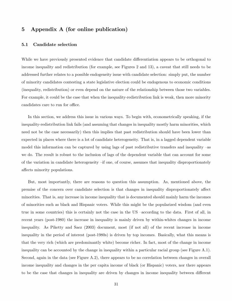
5 Appendix A (for online publication)

5.1 Candidate selection

While we have previously presented evidence that candidate differentiation appears to be orthogonal to

income inequality and redistribution (for example, see Figures 2 and 13), a caveat that still needs to be

addressed further relates to a possible endogeneity issue with candidate selection: simply put, the number

of minority candidates contesting a state legislative election could be endogenous to economic conditions

(inequality, redistribution) or even depend on the nature of the relationship between those two variables.

For example, it could be the case that when the inequality-redistribution link is weak, then more minority

candidates care to run for offi ce.

In this section, we address this issue in various ways. To begin with, econometrically speaking, if the

inequality-redistribution link fails (and assuming that changes in inequality mostly harm minorities, which

need not be the case necessarily) then this implies that past redistribution should have been lower than

expected in places where there is a lot of candidate heterogeneity. That is, in a lagged dependent variable

model this information can be captured by using lags of past redistributive transfers and inequality —as

we do. The result is robust to the inclusion of lags of the dependent variable that can account for some

of the variation in candidate heterogeneity —if one, of course, assumes that inequality disproportionately

affects minority populations.

But, most importantly, there are reasons to question this assumption. As, mentioned above, the

premise of the concern over candidate selection is that changes in inequality disproportionately affect

minorities. That is, any increase in income inequality that is documented should mainly harm the incomes

of minorities such as black and Hispanic voters. While this might be the popularized wisdom (and even

true in some countries) this is certainly not the case in the US —according to the data. First of all, in

recent years (post-1980) the increase in inequality is mainly driven by within-whites changes in income

inequality. As Piketty and Saez (2003) document, most (if not all) of the recent increase in income

inequality in the period of interest (post-1980s) is driven by top incomes. Basically, what this means is

that the very rich (which are predominantly white) become richer. In fact, most of the change in income

inequality can be accounted by the change in inequality within a particular racial group (see Figure A.1).

Second, again in the data (see Figure A.2), there appears to be no correlation between changes in overall

income inequality and changes in the per capita income of black (or Hispanic) voters, nor there appears

to be the case that changes in inequality are driven by changes in income inequality between different

31

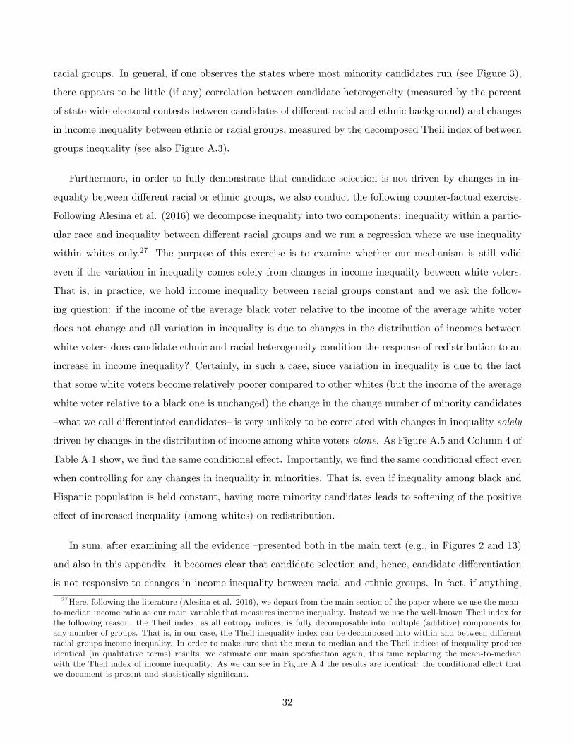
racial groups. In general, if one observes the states where most minority candidates run (see Figure 3),

there appears to be little (if any) correlation between candidate heterogeneity (measured by the percent

of state-wide electoral contests between candidates of different racial and ethnic background) and changes

in income inequality between ethnic or racial groups, measured by the decomposed Theil index of between

groups inequality (see also Figure A.3).

Furthermore, in order to fully demonstrate that candidate selection is not driven by changes in in-

equality between different racial or ethnic groups, we also conduct the following counter-factual exercise.

Following Alesina et al. (2016) we decompose inequality into two components: inequality within a partic-

ular race and inequality between different racial groups and we run a regression where we use inequality

within whites only.27 The purpose of this exercise is to examine whether our mechanism is still valid

even if the variation in inequality comes solely from changes in income inequality between white voters.

That is, in practice, we hold income inequality between racial groups constant and we ask the follow-

ing question: if the income of the average black voter relative to the income of the average white voter

does not change and all variation in inequality is due to changes in the distribution of incomes between

white voters does candidate ethnic and racial heterogeneity condition the response of redistribution to an

increase in income inequality? Certainly, in such a case, since variation in inequality is due to the fact

that some white voters become relatively poorer compared to other whites (but the income of the average

white voter relative to a black one is unchanged) the change in the change number of minority candidates

—what we call differentiated candidates—is very unlikely to be correlated with changes in inequality solely

driven by changes in the distribution of income among white voters alone. As Figure A.5 and Column 4 of

Table A.1 show, we find the same conditional effect. Importantly, we find the same conditional effect even

when controlling for any changes in inequality in minorities. That is, even if inequality among black and

Hispanic population is held constant, having more minority candidates leads to softening of the positive

effect of increased inequality (among whites) on redistribution.

In sum, after examining all the evidence —presented both in the main text (e.g., in Figures 2 and 13)

and also in this appendix—it becomes clear that candidate selection and, hence, candidate differentiation

is not responsive to changes in income inequality between racial and ethnic groups. In fact, if anything,

27Here, following the literature (Alesina et al. 2016), we depart from the main section of the paper where we use the mean-to-median income ratio as our main variable that measures income inequality. Instead we use the well-known Theil index forthe following reason: the Theil index, as all entropy indices, is fully decomposable into multiple (additive) components forany number of groups. That is, in our case, the Theil inequality index can be decomposed into within and between differentracial groups income inequality. In order to make sure that the mean-to-median and the Theil indices of inequality produceidentical (in qualitative terms) results, we estimate our main specification again, this time replacing the mean-to-medianwith the Theil index of income inequality. As we can see in Figure A.4 the results are identical: the conditional effect thatwe document is present and statistically significant.

32

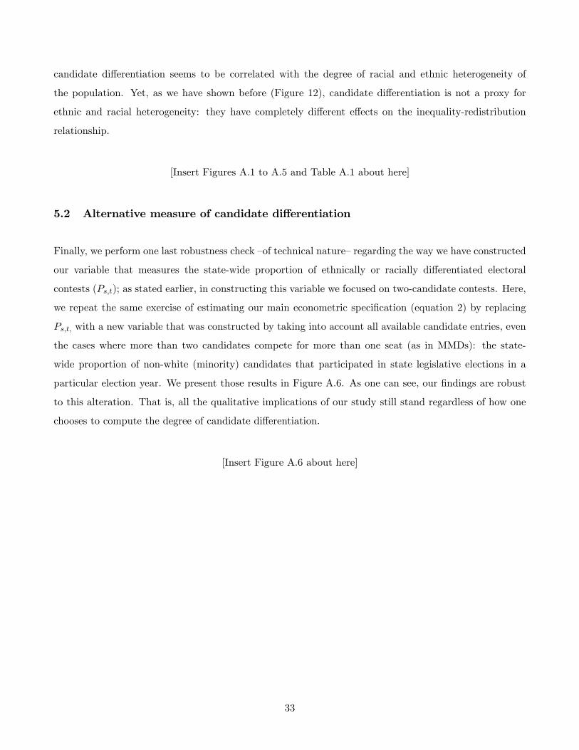
candidate differentiation seems to be correlated with the degree of racial and ethnic heterogeneity of

the population. Yet, as we have shown before (Figure 12), candidate differentiation is not a proxy for

ethnic and racial heterogeneity: they have completely different effects on the inequality-redistribution

relationship.

[Insert Figures A.1 to A.5 and Table A.1 about here]

5.2 Alternative measure of candidate differentiation

Finally, we perform one last robustness check —of technical nature—regarding the way we have constructed

our variable that measures the state-wide proportion of ethnically or racially differentiated electoral

contests (Ps,t); as stated earlier, in constructing this variable we focused on two-candidate contests. Here,

we repeat the same exercise of estimating our main econometric specification (equation 2) by replacing

Ps,t, with a new variable that was constructed by taking into account all available candidate entries, even

the cases where more than two candidates compete for more than one seat (as in MMDs): the state-

wide proportion of non-white (minority) candidates that participated in state legislative elections in a

particular election year. We present those results in Figure A.6. As one can see, our findings are robust

to this alteration. That is, all the qualitative implications of our study still stand regardless of how one

chooses to compute the degree of candidate differentiation.

[Insert Figure A.6 about here]

33

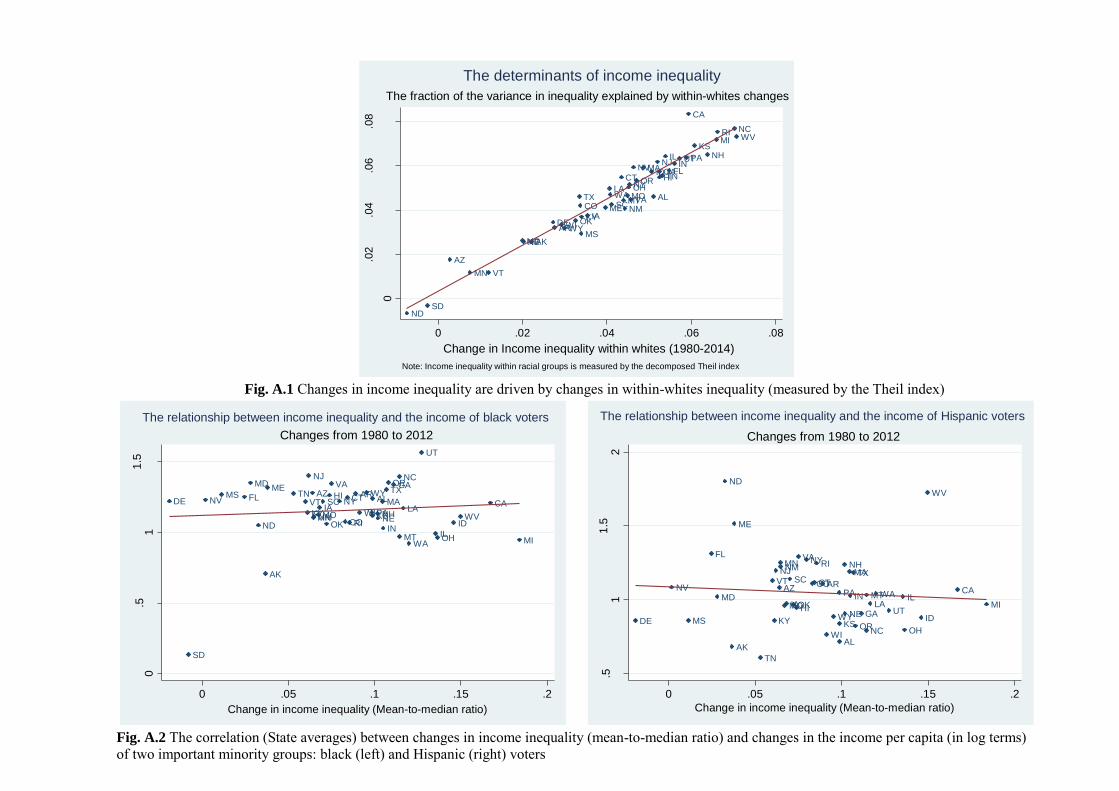
Fig. A.1 Changes in income inequality are driven by changes in within-whites inequality (measured by the Theil index)

Fig. A.2 The correlation (State averages) between changes in income inequality (mean-to-median ratio) and changes in the income per capita (in log terms) of two important minority groups: black (left) and Hispanic (right) voters

AL

AK

AZ

AR

CA

CO

CT

DE

FLGAHI

ID

ILIN

IA

KS

KY

LA

ME

MD

MA

MI

MN

MS

MOMT

NE

NV

NHNJ

NM

NY

NC

ND

OH

OK

OR

PA

RI

SC

SD

TN

TX

UT

VT

VAWA

WV

WIWY

0

.02

.04

.06

.08

Cha

ng

e in

inco

me in

eq

ua

lity (

Th

eil

inde

x)

0 .02 .04 .06 .08

Change in Income inequality within whites (1980-2014)

Note: Income inequality within racial groups is measured by the decomposed Theil index

The fraction of the variance in inequality explained by within-whites changes

The determinants of income inequality

AL

AK

AZ ARCA

CO

CTDE FL

GA

HI

ID

ILIN

IAKSKY

LA

MEMD

MA

MI

MN

MS

MO

MT

NE

NV

NH

NJ

NM

NY

NC

ND

OH

OK

OR

PARI

SC

SD

TN TX

UT

VT

VA

WA

WVWI

WY

0.5

11

.5

Cha

ng

e in

the

p.c

. in

co

me (

in log

s)

of bla

ck v

ote

rs

0 .05 .1 .15 .2

Change in income inequality (Mean-to-median ratio)

Changes from 1980 to 2012

The relationship between income inequality and the income of black voters

ALAK

AZ ARCA

COCT

DE

FL

GAHI

ID

ILINIA

KSKY

LA

ME

MD

MA

MI

MN

MS

MOMT

NE

NV

NHNJNM

NY

NC

ND

OH

OK

OR

PA

RI

SC

TN

TX

UT

VT

VA

WA

WV

WI

WY

.51

1.5

2

Cha

ng

e in

the

p.c

. in

co

me (

in log

s)

of H

ispa

nic

vo

ters

0 .05 .1 .15 .2

Change in income inequality (Mean-to-median ratio)

Changes from 1980 to 2012

The relationship between income inequality and the income of Hispanic voters

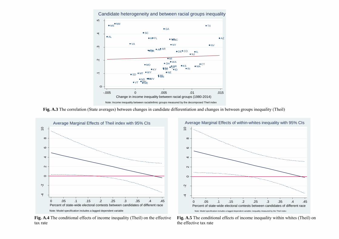
Fig. A.3 The correlation (State averages) between changes in candidate differentiation and changes in between groups inequality (Theil)

Fig. A.4 The conditional effects of income inequality (Theil) on the effective tax rate

Fig. A.5 The conditional effects of income inequality within whites (Theil) on the effective tax rate

AL

AK

AZ

ARCO

CT

DE

FL

GA

HI

ID

IL

IN

IA

KS

KY

ME

MD

MA

MI

MN

MS

MO

MT NE

NV

NH

NJ

NM

NY

NC

ND

OH

OK

ORPA RI

SC

SD

TN

TX

UT

VT

VA

WA

WV

WI

WY

0.1

.2.3

.4.5

Pe

rce

nt o

f sta

te-w

ide

co

nte

sts

be

twee

n c

an

did

ate

s o

f d

iffe

ren

t ra

ce

-.005 0 .005 .01 .015

Change in income inequality between racial groups (1980-2014)

Note: Income inequality between racial/ethnic groups measured by the decomposed Theil index

Candidate heterogeneity and between racial groups inequality

-4-2

02

46

81

0

Eff

ective

tax r

ate

(in

%)

0 .05 .1 .15 .2 .25 .3 .35 .4 .45

Percent of state-wide electoral contests between candidates of different race

Note: Model specification includes a lagged dependent variable

Average Marginal Effects of Theil index with 95% CIs

-4-2

02

46

81

0

Eff

ective

tax r

ate

(in

%)

0 .05 .1 .15 .2 .25 .3 .35 .4 .45

Percent of state-wide electoral contests between candidates of different race

Note: Model specification includes a lagged dependent variable; inequality measured by the Theil index

Average Marginal Effects of within-whites inequality with 95% CIs

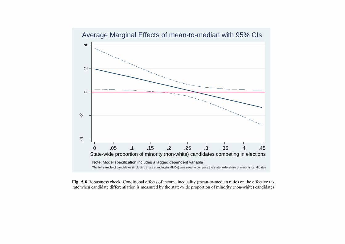
Fig. A.6 Robustness check: Conditional effects of income inequality (mean-to-median ratio) on the effective tax rate when candidate differentiation is measured by the state-wide proportion of minority (non-white) candidates

-4-2

02

4

Eff

ective

tax r

ate

(in

%)

0 .05 .1 .15 .2 .25 .3 .35 .4 .45

State-wide proportion of minority (non-white) candidates competing in elections

Note: Model specification includes a lagged dependent variable

The full sample of candidates (including those standing in MMDs) was used to compute the state-wide share of minority candidates

Average Marginal Effects of mean-to-median with 95% CIs

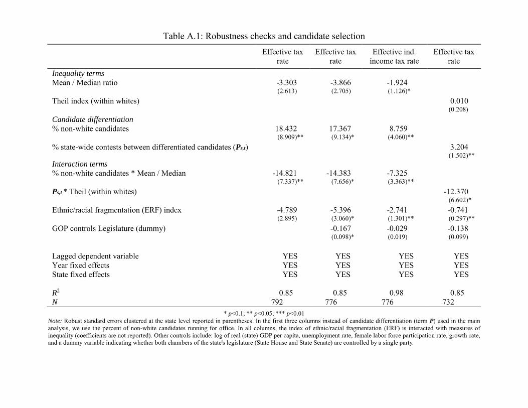
Table A.1: Robustness checks and candidate selection Effective tax

rate Effective tax

rate Effective ind.

income tax rate Effective tax

rate Inequality terms Mean / Median ratio -3.303 -3.866 -1.924 (2.613) (2.705) (1.126)* Theil index (within whites) 0.010 (0.208) Candidate differentiation % non-white candidates 18.432 17.367 8.759 (8.909)** (9.134)* (4.060)** % state-wide contests between differentiated candidates (Ps,t) 3.204

(1.502)** Interaction terms % non-white candidates * Mean / Median -14.821 -14.383 -7.325 (7.337)** (7.656)* (3.363)** Ps,t * Theil (within whites) -12.370 (6.602)* Ethnic/racial fragmentation (ERF) index -4.789 -5.396 -2.741 -0.741 (2.895) (3.060)* (1.301)** (0.297)** GOP controls Legislature (dummy) -0.167 -0.029 -0.138 (0.098)* (0.019) (0.099) Lagged dependent variable YES YES YES YES Year fixed effects YES YES YES YES State fixed effects YES YES YES YES R2 0.85 0.85 0.98 0.85 N 792 776 776 732

* p<0.1; ** p<0.05; *** p<0.01 Note: Robust standard errors clustered at the state level reported in parentheses. In the first three columns instead of candidate differentiation (term P) used in the main analysis, we use the percent of non-white candidates running for office. In all columns, the index of ethnic/racial fragmentation (ERF) is interacted with measures of inequality (coefficients are not reported). Other controls include: log of real (state) GDP per capita, unemployment rate, female labor force participation rate, growth rate, and a dummy variable indicating whether both chambers of the state's legislature (State House and State Senate) are controlled by a single party.

For Online Publication:

Appendix B: Data sources, variable definitions and coding

VARIABLE NAME

DESCRIPTION

SOURCE

efftax

Effective tax rate (in %) defined as the ratio of total (per-capita) tax receipts over (per-capita) income at the US State level

Own calculation using data from the US Census Bureau (tax receipts) and the regional data-base of the Bureau of

Economic Analysis (income data)

heter_q1

Ethnic heterogeneity (bottom quintile or gross earnings)

Own calculation using data on ethnicity/race and gross earnings from the US Census

Bureau (1979-2011)

heter_med

Ethnic heterogeneity (median quintile or gross earnings)

Own calculation using data on ethnicity/race and gross earnings from the US Census

Bureau (1979-2011)

heter_q5

Ethnic heterogeneity (top quintile or gross earnings)

Own calculation using data on ethnicity/race and gross earnings from the US Census

Bureau (1979-2011)

heter_tot

Aggregate ethnic heterogeneity (all income quintiles) at the US State level

Own calculation using data on ethnicity/race from the US

Census Bureau (1979-2011)

relheter

Relative ethnic heterogeneity (ratio) of poor (bottom quintile) vs. rich (top quintile)

Own calculation by taking the ratio of heter_q1 / heter_q5

relheter2

Relative ethnic heterogeneity (difference) of poor (bottom quintile) vs. rich (top quintile)

Own calculation by calculating the difference between heter_q1- heter_q5

relheter 3

Relative ethnic heterogeneity (ratio) of median quintile vs. rich (top quintile)

Own calculation by taking the ratio of heter_med / heter_q5

relheter 4

Relative ethnic heterogeneity (difference of median quintile vs. rich (top quintile)

Own calculation by calculating the difference between heter_med - heter_q5

stran

Social transfer rate (in %) defined as the ratio of total (per-capita) social transfers over (per-capita) income at the state-level

Own calculation using data from the regional data-base of the Bureau of Economic

Analysis (social transfers and income data)

atkin05

Atkinson index of income inequality at the US state level

From Frank (2007) data-base constructed using data from the IRS (SOE) data on gross personal income

gini

Gini coefficient of income inequality at the US state level

From Frank (2007) data-base constructed using data from the IRS (SOE) data on gross personal income

rmeandev

Relative mean deviation of income at the US state level

From Frank (2007) data-base constructed using data from the IRS (SOE) data on gross personal income

gdp_pc

Average real income (per-capita) at the US state level

From the regional accounts data-base of the Bureau of

Economic Analysis

gop_control

Binary variable indicating the overall control of the State legislature (both chambers) by the Republican party (GOP)

From National Conference of

State Legislatures (NCSL)

property_tax

Total property tax receipts

Data from the US Census

Bureau

tot_inc_tax

Total income tax receipts

Data from the US Census

Bureau

ind_inc_tax

Total individual income tax receipts

Data from the US Census

Bureau

corp_inc_tax

Total corporate income tax receipts

Data from the US Census

Bureau

efftax_property

Effective property tax-rate (calculated as efftax above)

Own calculation using data from the US Census Bureau (tax receipts) and the regional data-base of the Bureau of

Economic Analysis (income data)

efftax_inc

Effective income (overall) tax-rate (calculated as efftax above)

Own calculation using data from the US Census Bureau (tax receipts) and the regional data-base of the Bureau of

Economic Analysis (income data)

efftax_ind_inc

Effective individual income tax-rate (calculated as efftax above)

Own calculation using data from the US Census Bureau (tax receipts) and the regional data-base of the Bureau of

Economic Analysis (income data)

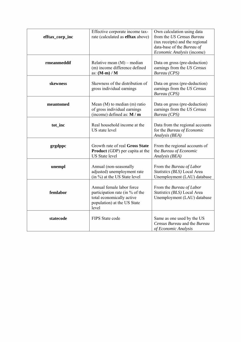
efftax_corp_inc

Effective corporate income tax-rate (calculated as efftax above)

Own calculation using data from the US Census Bureau (tax receipts) and the regional data-base of the Bureau of

Economic Analysis (income)

rmeanmeddif

Relative mean (M) – median (m) income difference defined as: (M-m) / M

Data on gross (pre-deduction) earnings from the US Census

Bureau (CPS)

skewness

Skewness of the distribution of gross individual earnings

Data on gross (pre-deduction) earnings from the US Census

Bureau (CPS)

meantomed

Mean (M) to median (m) ratio of gross individual earnings (income) defined as: M / m

Data on gross (pre-deduction) earnings from the US Census

Bureau (CPS)

tot_inc

Real household income at the US state level

Data from the regional accounts for the Bureau of Economic

Analysis (BEA)

grgdppc

Growth rate of real Gross State

Product (GDP) per capita at the US State level

From the regional accounts of the Bureau of Economic

Analysis (BEA)

unempl

Annual (non-seasonally adjusted) unemployment rate (in %) at the US State level

From the Bureau of Labor

Statistics (BLS) Local Area Unemployment (LAU) database

femlabor

Annual female labor force participation rate (in % of the total economically active population) at the US State level

From the Bureau of Labor

Statistics (BLS) Local Area Unemployment (LAU) database

statecode

FIPS State code

Same as one used by the US Census Bureau and the Bureau

of Economic Analysis