CIV ENG 471-1 Transportation Systems Analysis

Department of Civil and Environmental Engineering Northwestern University

Winter 2006

Urban Travel Forecasting

Course Notes

© 2006

by

David Boyce

Adjunct Professor Department of Civil and Environmental Engineering

Northwestern University Evanston, Illinois

2149 Grey Avenue

Evanston, Illinois 60201 USA d-boyce@northwestern.edu

Phone: 847-570-9501 Fax: 775-587-2308

Minor revisions – November 2006

ii

Preface

These Course Notes stem from teaching graduate courses in urban travel forecasting at the University of Pennsylvania, 1968-1976, the University of Illinois at Urbana-Champaign, 1977-1987, and the University of Illinois at Chicago, 1988-2002. The notes began to take their present form during courses taught in 2003 at the National University of Singapore, the University of Canterbury, Christchurch, New Zealand, and the University of Pennsylvania, Philadelphia. Subsequent additions and revisions of the notes were made in teaching courses at Northwestern University in 2005 and 2006. I gratefully acknowledge my ongoing collaboration with Hillel Bar-Gera, Ben-Gurion University of the Negev, Israel, for his many contributions to my understanding of combined models of travel and route choice. I thank the following students for their assistance in preparing the current version of these Notes: Nan Liu, National University of Singapore, Jeff Casello, University of Pennsylvania, and Vincent Bernardin, Jr., Northwestern University. Biljana Dekic prepared the GIS maps in Section 3. Qian Xiong and Frederik Noeth, University of Illinois at Chicago, contributed related materials. I also thank the graduate students in these courses, too numerous to mention, for their comments, criticisms and patience with my efforts. I am grateful for the opportunity to teach my urban travel forecasting course during the period 2003-2006, which was facilitated by the following colleagues: Professor Der-Horng Lee, National University of Singapore; Professor Alan Nicholson, University of Canterbury; Professor Vukan Vuchic, University of Pennsylvania; and Professor Joseph Schofer, Northwestern University. These Course Notes may be used for research and teaching purposes with proper attribution of the source. Comments and criticisms are most welcome, as the revision and expansion of these notes is an ongoing activity. David Boyce April 2006

iii

Table of Contents 1. Urban Travel Forecasting – The General Problem 1 1.1 Requirements and Context 1 1.2 General Formulation of the Urban Travel Forecasting Problem 4 1.3 Fixed Point Problem 5 1.4 Example of a Fixed Point Formulation of a Travel Model 6 1.5 Sequential Travel Forecasting Procedure 8 References 11 Exercise 11 A. Appendix on Optimization and Equilibrium Methods 12 A.1 Preliminaries 12 A.2 Minima and Convexity 14 A.3 Optimization with Equality Constraints 15 A.4 Optimization with Inequality Constraints 17 A.5 More General Formulations 20 A.6 Examples of Constrained Optimization Problems 23 Exercises 25 2. Auto Route Choice Principles 26 2.1 User-Optimal Route Choice 26 2.2 NCP and VIP Formulations 33 2.2 System-Optimal Route Choice 36 2.4 Solution Algorithm for the Two-Link Problem based on the Frank-Wolfe Method 38 2.5 Braess’s Paradox 43 References 43 Exercises 44 3. Road and Transit Network Route Choice 54 3.1 Network Concepts and Shortest Route Algorithms 54 3.2 Auto Route Choice on a Network with Fixed OD Flows 56 3.3 Solution Algorithm for UO-TAP based on the Frank-Wolfe Method 59 3.4 Overview of the Origin-Based Traffic Assignment Algorithm 61 3.5 Case Study of Convergence of UO TAP 70 3.6 Dynamic Route Choice on a Road Network 81 3.4 Transit Route Choice 91 References 91 4. Mode Choice 93 4.1 Deterministic Mode Choice 93 4.2 Dispersion Constraint 95 4.3 Combined Mode and Route Choice Models 99 4.4 Properties of the Logit Model 100 4.5 Nested Logit Model and Composite Costs 102 Exercises 104

iv

5. Origin-Destination Choice (Trip Distribution) 106 5.1 Model Derivation 107 5.2 Computation of Ap and Bq 109 5.3 Calibration of Travel Deterrence Parameters 110 5.4 Form of the Deterrence Function 111 5.5 Extension to Tours 113 5.6 Extension to Time Intervals 117 References 119 Exercises 124 6. Combined Models and Feedback 125 6.1 Problem Statement 125 6.2 Formulation of the Combined Model 126 6.3 Evans Algorithm for the Combined Model 127 6.4 Case Study – An Application of the Combined Model to the Chicago Region 131 6.5 Solving the Sequential Procedure with Feedback 142 6.6 Some Practical Issues 157 References for Further Study 159

1

1. Urban Travel Forecasting – The General Problem We begin with a rather general statement of the problem and requirements for an urban travel forecasting method for a large, congested urban area. In an effort to address the core issues facing transportation planners today and in the future, we largely ignore past practice and the constraints imposed by computers and incomplete understanding of the problem. Although our intent is to be reasonably comprehensive, some aspects will be ignored or omitted. 1.1 Requirements and Context We accept the following ground rules for our model in order to conform to current and recent practice: 1. The urban region is divided into small, relatively homogeneous areas called zones. The zone

size depends on the density of development, so that activity levels per zone are relatively similar.

2. Urban activities in zones are described in terms of the following types of variables:

a. residential population and households; b. employment c. education (primary, secondary, higher) and day care; d. shopping and personal and business services; e. recreation.

3. Facilities for urban activities are described in terms of land and building area:

a. housing; b. workplaces; c. schools and colleges; d. shopping and services; e. recreational facilities: parks, stadiums, theaters. etc.

4. Travel occurs on two types of transportation modes:

a. private vehicle/roadway/traffic control system; b. public transit/roadway or railway/operations plan In addition, various types of trucks use the roadway system. These transportation systems are represented as networks consisting of nodes, links, link attributes, and in the case of transit, routes of scheduled services. The service characteristics of links, which are one type of link attribute, depend upon a number of fixed variables: a. physical roadway and vehicle characteristics: length, number and width of lanes, grades, etc., and transit station spacing and vehicle performance; b. control and operations plans: speed limits, signal settings, road tolls; service frequencies and operating speeds, transit fares;

2

Other variables related to travel flows (demand) also determine service characteristics: c. vehicle flows in the case of private vehicles, and number of boardings and alightings at stops per unit time, in the case of public transit. Taken together, these variables determine the performance characteristics of an individual link. In general, they are of the form: link travel time = f(vehicle and roadway characteristics, operations plan, flows), where the underlining denotes that these variables are fixed. Such performance functions are often confused with supply functions. For a supply function, in contrast, the vehicle and roadway characteristics, and the operations plan are not fixed, but rather are decision variables of the operator or supplier. In travel forecasts, variations in supplier are typically not represented. For example, adjustments to signal timing and transit service frequencies are not generally made in response to the forecasted travel choices.

5. Travel between daily activities (residing, working, eating, shopping, schooling, recreating)

may be described in terms of pairs of activities linked by traveling; for example: a. home-work; b. work-eat meal; c. work-shop; d. shop-home; Over the 24-hour weekday, travel described in terms of several activities make up a sequence of trips for various purposes, or trip chain. Naturally, the duration of the activity, and the time required for travel, determine the geographic range of activities visited. Therefore, travel may be described in terms of individual trips, called trip-based, or sequences of trips and activities, called activity-based, or sometimes trip chaining. Most of these notes address trip-based models, but trip chain models are described in Section 5.

6. Whether travel occurs by private car, either alone or with others, or by public transit, depends

on the availability of each mode, and their relative service times and monetary costs, as well as less tangible factors like comfort and convenience.

7. The timing of travel during the day also depends on constraints imposed by activity

schedules, and the travel conditions on the private and public networks. 8. Travel may be assumed to occur during a given period of the 24-hour day, such as the

morning peak commuting period. To convert actual trips, with their specific departure and arrival times, into flows (persons/unit time), we need a conversion procedure, such as one of the following: a. all travelers departing from home and going to work during 6-9 am are counted as flows

in persons/hour; b. all travelers arriving at work from home during 6-9 am are counted as flows in

persons/hour;

3

c. all travelers in the network between 6 and 9 am are counted as whole or partial flows in persons/hour.

The following space-time diagram seeks to illustrate the problem. As will become clear, either explicitly or implicitly when we examine specific models, the variables of interest are flows, not trips or trip chains. In this example, 3 travelers depart during 6-9 am; 3 travelers arrive during 6-9 am, but they are different travelers. About 3.4 travelers are in the network from 6-9 am. The different slopes of the trajectories denote that home and work are separated differently for each traveler, and also that they have different speeds in the network. Flows can be compiled from household travel surveys based on these various definitions. These issues arise from seeking to represent a dynamic phenomenon as a static one.

From the viewpoint of transportation system planning, facility design, operations planning and conforming with air quality regulations, we require the forecasts of the following variables for a given transportation system/activity pattern scenario: 1. flows of private cars, trucks and transit vehicles on the road network for the most congested

periods of the 24-hour weekday (the morning and evening peak commuting periods) and for other longer periods during which travel conditions are reasonably stable;

2. flows of persons on the public transit network by service type (e.g., bus, rapid transit,

commuter rail) by time period of the 24-hour weekday;

5 am 6 am 7 am 8 am 9 am

home

work

space

time

4

3. flows of persons from origin zone to destination zone by private and public modes and time period, and by route, if available and pertinent.

A capability to examine changes in these flows in response to changes in network capacity and service attributes, monetary costs (e.g., fuel, tolls, fares, parking fees), and changes in zonal activity levels is also implied. 1.2 General Formulation of the Urban Travel Forecasting Problem Consider the following definitions and notation: dpqmr person flow (trips/hour) from origin zone p to destination zone q on route r of mode m Rp number of persons residing in zone p Wq number of employees working in zone q Eq number of persons attending school or college in zone q Sq level of shopping and service activity in zone q cpqmr generalized cost of travel from zone p to zone q on route r of mode m

,1=apqmrδ if link a belongs to route r of mode m from zone p to zone q;

0, otherwise fa flow of vehicles per hour on link a ca(fa) generalized cost of travel per vehicle on link a at flow fa Lm set of links in the network of mode m M set of modes Rpqm set of routes connecting zone p to zone q by mode m ηm occupancy of mode m in persons per vehicle The general problem we wish to solve may be stated as follows:

mpqm Rr

apqmrpqmr

ma

La

apqmraapqmr

pqmrqqqppqmr

Ladf

rmqpfcc

rmqpcSEWRfd

pqm

m

∈⋅≡

⋅≡

=

∑ ∑

∑

∈

∈

all for

all for

all for

,1

,,,,)(

,,,),,...,,,,(

δη

δ

Note that the last two expressions are definitions, which are illustrated by the following figures.

5

Definition of Interzonal Travel Cost Definition of Link Flow

Replacing these variables by their definitions, we obtain:

⎥⎥⎦

⎤

⎢⎢⎣

⎡⋅⎟⎟⎠

⎞⎜⎜⎝

⎛⋅= ∑ ∑ ∑

∈ ∈m pqmLa

apqmr

pqm Rr

apqmrpqmr

maqqppqmr dcSERfd δδη1,...,,,

Therefore, pqmrd is a function of itself through its accumulated effect on link flows, and therefore on link costs. Hence, the problem we seek to solve has the structure of a fixed point problem. 1.3 Fixed Point Problem The fixed point problem is to find for the function ( )xf a value of

where X is the constraint space on variable x. An example is shown below.

zone p

zone q

c1(f1)

c2(f2)

c3(f3)

( ) ( ) ( )3322111 fcfcfcc pqm ++=

link a

zone p

zone p'

zone p"

zone q

zone q'

zone q" qpqpqpqpqpqppqa dddddddf ′′′′′′′′′′′′′ +++⋅⋅⋅++++=

( )∗∗ =∈ xfxXx such that

6

1.4 Example of a Fixed Point Formulation of a Travel Model The objective of this subsection is to illustrate the above ideas with a small example. Consider a travel forecasting problem with two nodes, A and B, connected by a single link from A to B. Travel from A to B in vehicles per hour is denoted by d, and the cost of travel is denoted by c. Assume the following demand function defines d: ( )cgdd o= where od is the total travel demand that would occur in the absence of any travel cost (c = 0), and ( )cg denotes a positive and decreasing function of travel cost. Examples of positive decreasing functions are:

( )( ) ( )( ) ( )( )cccg

ccgcbacg

lnexp

exp

3

2

1

⋅−==

⋅−=⋅−=

− α

βα

where a, b, αβ , are parameters with positive values. Note that these functions are all positive and decreasing over values of .0≥c Next, we need to define a functional relationship ( )⋅h between link flow and link travel cost; that is, we need a performance function.

A B

d

7

Since there is only one link, the flow f must equal d in this static model. Assume that ( ) ( )dhfhc == is a positive, increasing function of f. Examples of positive, increasing functions are:

( )( ) ( )4

2

1

1 fscfh

fsrfh

o

n

⋅+=

⋅+=

where r and s are positive parameters, and f is raised to the power of n. The second function is widely known as the BPR function, which was originally proposed by engineers at the U.S. Bureau of Public Roads about 1960 with ,/15.0 4capacitys = based on very little data. Now, let us combine these functions to form a simultaneous model of travel demand and travel cost: ( )( ) ( )( )dhgdfhgdd oo == Thus, we see that travel demand from A to B is a function that depends on that demand itself plus several parameters. For example,

( )( ) ( )( )( )( ) ( ) ( )

( ) sccdddddsccd

fscdfhgdd

oooo

no

nooo

nooo

⋅⋅≡′⋅−⋅≡′⋅′−⋅′=⋅⋅⋅−⋅⋅−⋅=

⋅+−⋅==

ββββββ

β

and exp ifexpexpexp

1exp

Such a formulation is called a fixed point problem. This class of problems is known to have a solution (existence) under rather general conditions. Under somewhat more restrictive conditions, there exists only one solution (uniqueness). Such properties are important for solving large-scale versions of the problem. Next, consider a graphical representation of the example. Let ,01.0,hour vehicles/1000 == βod

min. 30 ,500/15.0 4 == ocs Plot ( ) ( )4exp dddf o ⋅′−⋅′= β vs. d, and also plot ( ) .ddf = The intersection of these two equations is the fixed point ,∗d which is the solution to the problem. It may also be regarded as an equilibrium point.

8

Fixed Point Function Relating OD Flow to Link Flow

0

200

400

600

800

0 200 400 600 800 1000 1200 1400 1600 1800

f - Link Flow (vehicles/hour)

d -

OD

Flo

w (v

ehic

les/

hour

)

1.5 Sequential Travel Forecasting Procedure Because of the complexity of solving the general travel forecasting problem for its equilibrium, the problem was simplified by converting it into a sequence of steps or stages. This simplification occurred in the very first transportation planning studies, and continues to this day. This decomposition of such a problem is appropriate if the equilibrium solution is maintained. Unfortunately, this requirement was not even understood, much less observed in practice. Recently, efforts to solve the four-step procedure with feedback have recognized this requirement, but generally not fulfilled it completely and rigorously. The four-step procedure is described below as background for the consideration of the general problem in these notes. The equilibrium problem described above was conceptually solved as a sequence of four procedures. The notation is the same as defined earlier. 1. Trip Generation Determine the flow of travelers per day leaving or entering each zone as a

function of zonal activity levels; also determine the auto availability for these trips.

qSEWfD

pRfO

qqqq

pp

allfor ,...),,(

allfor ,...)(

=

=

2. Trip Distribution Determine the flow of travelers per day pqd from origin zone p to destination zone q

( )pqqppq cDOfd ,,=

⎟⎟⎠

⎞⎜⎜⎝

⎛⎟⎟⎠

⎞⎜⎜⎝

⎛⋅−⋅= 4

4

500045.0exp8.740 fd

d = f

0.651* =d

9

where pqc is the generalized travel cost from origin zone p to destination zone q, determined in some convenient way, such as finding shortest routes over the roadway network for zero flow conditions. Assume pqd is directly proportion to pO and qD , and inversely proportional to pqc . 3. Modal Split Allocate flows of travelers to modes.

( )pqmpqpqm cdfd ,= where m belongs to the set of modes serving zone pair pq. 4. Traffic Assignment Allocate flows of interzonal travelers by mode to routes

( )pqmrpqmpqmr cdfd ,= where r belongs to the set of routes serving zone pair pq by mode m. Recall that ∑

∈

⋅≡mLa

apqmraapqmr rmqpfcc ,,, allfor ,)( δ

where ( ) =aa fc generalized cost of travel per vehicle on link a at flow fa

,1=apqmrδ if link a belongs to route r of mode m from zone p to zone q;

0, otherwise Note the nature of the terminology used, as if travel behavior was a kind of mechanistic process. Our notation implies:

∑

∑=

=

rpqmrpqm

mpqmpq

dd

dd

The relation of the four models (procedures) is shown in the following figure. Often the questions of the source of the interzonal travel cost pqc and its relation to

( )aapqmr fcc and is not addressed by this procedure. In other words, pqmrc is assumed to be available in the trip distribution and modal split steps, but is determined only in the traffic assignment step. The dashed feedback arrow solves this problem conceptually, but leaves unanswered the question of whether the implied iterations converge to a stable solution. Until the feedback requirement imposed by the U. S. Intermodal Surface Transportation Efficiency Act of 1991 (ISTEA), such iterations were only rarely attempted in the United States. Another issue is the time period of the travel activity. In the past, most forecasts were prepared for the 24-hour weekday. This was convenient since origins and destinations tend to balance

10

over 24 hours. The difficulty with the 24-hour concept is that travel costs vary over this period due to congestion during peak travel periods, which is the very congestion we are concerned with predicting. One approach to this problem is to compute a peaking factor, i.e. the ratio of peak-hour flow to 24-hour flow, typically, about 0.1. Such factors were used to convert hourly capacity into 24-hour capacity,

Sequential Travel Forecasting Procedure or 24-hour link flows into hourly flows. The difficulty, of course, is that the factor depends on the level of congestion. An alternative approach is to factor 24-hour trips to hourly trip flows using observed data on trip departures and perform the analysis for selected time-of-day periods, say the peak morning and evening travel periods. All such models are static flow models, because the travel times and flows are considered to be constant during the period of analysis. They are also macroscopic, since there is no concept of individual trips or vehicles moving through the network in these models. The peak period should be long enough, therefore, that it is reasonable to consider that trips can move from origin to destination. Usually, at least one hour is used. Other than the conceptual issue that travel times may exceed the period length, it doesn't matter. For the same reason, flows are said to propagate instantaneously from origin to destination. In other words, in the model the flows from origins to destinations either exist or they don’t exist.

Traffic Assignment

Modal Split

Trip Distribution

Trip Generation

11

References J. de D. Ortúzar and L. G. Willumsen (2001) Modelling Transport, 3rd edition, Wiley; pp. 1-9 for discussion of demand and supply functions. M. Manheim (1979) Fundamentals of Transportation Systems Analysis, Vol. 1, MIT Press, Cambridge, MA; especially Ch. 7. Exercise 1. Consider the following generalized cost equation. Note that the distance term does not depend on link flow.

The second term based on distance traveled is assumed to represent the monetary cost of travel, whereas the first term is assumed to represent the disutility of time. For route choice, assume that travelers only consider travel time, and not monetary cost in making their choices. However, for mode and OD choice, they consider both time and monetary costs in computing their generalized cost. Define a more detailed version of the “General Problem” which implements these assumptions. Keep in mind this is a conceptual model, so the point is the concepts, not the mathematics. If you wish, give your answer in words, rather than equations.

( ) ( )( )( )

leminutes/mi tontsminutes/ce toscents/mile fromfactor conversion a ,centmin

milecents

(miles) link on distance travel(minutes) flowat link on time travel

(minutes) flowat link on travelofcost dgeneralize where

⎟⎠⎞

⎜⎝⎛⋅⎟

⎠⎞

⎜⎝⎛=

===

⋅+=

γ

γ

adfaft

fafcdftfc

a

aaa

aaa

aaaaa

12

Appendix - Optimization Methods The objective of these notes is to introduce informally the methods needed to formulate and solve travel forecasting models as constrained optimization problems and more general approaches. The methods begin with unconstrained optimization from differential calculus, and proceed to the method of Lagrange multipliers (optimization with equality constraints). This classic approach is then extended to inequality and non-negativity constraints based on the Karush-Kuhn-Tucker Theorem (KKT). The conditions for existence and uniqueness of solutions are then stated. The application of KKT method of network equilibrium problems often leads to assumptions that are not satisfied by the application of interest. In this event, either restricted assumptions are made, or a more general method based directly on the equilibrium conditions of interest is applied. One of these approaches is the nonlinear complementarity problem; another is the variational inequality problem, and the most general is the fixed point problem. These methods are introduced next, again in an informal manner. Further readings: R.E. Miller, Optimization, Wiley, New York, 2000. (introductory and less formal) M.S. Bazaraa, H.D. Sherali and C.M. Shetty, Nonlinear Programming, Wiley, New York, 1993.

(more formal and advanced) M. Patriksson, The Traffic Assignment Problem, Models and Methods, VSP, Utrecht, 1994,

Section 3.1. A.1 Preliminaries 1. Functions Let y = f(x) be a continuous function describing a relationship between scalars y and x.

13

If x is a vector of length n, then the function is a surface, possibly in n+1 dimensions. 2. Derivatives Consider

x

xfxxfxx

xfxfxy

∆−∆+

=−−

=∆∆ )()()()( 00

01

01

This equation describes ∆y, the change in y, in relation to ∆x, the change in x; then the derivative is defined as:

xyxf

dxdy

xx ∆

∆=′=⎟

⎠⎞

⎜⎝⎛

→∆ 00 lim)(0

3. Tangents and slopes The slope of the tangent (a line just touching f(x) and not intersecting it) to the function at 0x is equal to the derivative at 0x . 4. Taylor series approximation An approximation to f(x) at 0x can be found to any degree of accuracy, if the derivatives are known, as follows:

14

⋅⋅⋅+′′⎟⎠⎞

⎜⎝⎛+′+≈+ 2

0000 ))((!2

1)()()( dxxfdxxfxfdxxf

A.2 Minima and Convexity 1. Minima (maxima)

The minimum (maximum) of a function occurs at the point(s) x* where the first derivative equals zero.

Convex function with minimum at 0 Concave function with maximum at 0 A zero-valued derivative is a necessary condition for a minimum or maximum point if

)( +∞<<−∞ x . If ),( xxx << then the minima or maxima may occur at the interval boundaries, where x denotes the minimum value of x, and x denotes the maximum value. To determine if the point is a minimum or a maximum, we need to consider the second derivative,

).()()/( xfdx

xfddx

dxdyd ′′=′

=

The second necessary condition for a minimum (maximum) is that ).0)((0)( ** ≤′′≥′′ xfxf In addition, there are similar sufficient conditions. 2. Convexity (concavity) A function is strictly convex (strictly concave) if a straight line joining two points lies above (below) the function. If the line coincides with the function, it is only convex (concave). Hence, a linear function is both convex and concave. Likewise, consider a line tangent to f(x) at x ; if f(x) lies above (below) the tangent, the function is convex (concave).

15

3. Partial derivatives

For multi-dimensional variables (x), the partial derivative ix

f∂∂ )(x with respect to ix is the

derivative of f(x) treating all variables other than ix as constants, where T denotes transpose. The gradient of a function is a vector containing the first partial derivatives of the function:

( ). where,)()()( 1

T

1n

n

xxx

fx

ff ⋅⋅⋅=⎟⎟⎠

⎞⎜⎜⎝

⎛∂∂⋅⋅⋅

∂∂

=∇ xxxx

The Hessian of a function is the symmetric matrix of second partial derivatives

( ) ( )

( ) ( )⎟⎟⎟⎟⎟⎟

⎠

⎞

⎜⎜⎜⎜⎜⎜

⎝

⎛

∂∂∂⋅⋅⋅

∂∂∂

⋅⋅∂∂

∂⋅⋅⋅

∂∂∂

=

nnn

n

xxf

xxf

xxf

xxf

Hxx

xx

2

1

2

1

2

11

2

4. Minimum of a multi-dimensional function The necessary conditions for a convex function f(x*) to achieve its minima at x* are: ( ) .0x =∇ ∗f To determine if the point is a minimum (convex) or maximum (concave), certain conditions involving the Hessian must be met. In this course we will generally know whether the function is convex or not, so this condition is not stressed. A.3 Optimization with Equality Constraints 1. Single equality constraint We first consider the problem of finding the minimum of a convex function f(x) subject to a single equality constraint:

( )( )

( )( )Tnj xxxx

h

f

⋅⋅⋅⋅⋅⋅=

=

21 where

0:subject to

min

x

x

xx

To solve this problem, we form the Lagrangean function ( )λ,xL ( ) ( ) ( )xxx hfL ⋅−≡ λλ,

16

Note the similarity of ( )λ,xL to f(x) for values of x that satisfy h(x) = 0. Also, we make no assumption about the sign of the Lagrange multiplier λ . To find the necessary conditions for a minimum, we apply the same method as for an unconstrained minimization:

( ) ( ) ( ) njx

hx

fx

L

jjj

,...1,0,==

∂∂⋅−

∂∂

=∂

∂ xxx λλ

( ) ( ) 0,=−=

∂∂ xx hL

λλ

Thus, we obtain (n + 1) simultaneous equations in (n + 1) unknowns:

( ) ( )( ) 0=−

=∇⋅−∇x

0xx xx

hhf λ

where ( ) ( ) ( ) ( )⎟⎟⎠

⎞⎜⎜⎝

⎛

∂∂

=∇⎟⎟⎠

⎞⎜⎜⎝

⎛

∂∂

=∇jj x

hhx

ff xxxx xx ; .

Note we could also add h(x) to f(x); however, one standard convention is the form shown above. 2. Extension to several equality constraints

( )( )( ) nmmih

f

i <== ,,...1,0:s.t.

min

x

xx

Forming the Lagrangean function, we obtain,

( ) ( ) ( )∑=

⋅−=m

iii hfL

1, xxx λλ

The necessary conditions are:

( ) ( ) ( )

( ) ( ) mihL

njx

hx

fx

L

ii

m

i j

ii

jj

,...1,0,

,...1,0,1

==−=∂

∂

==∂

∂⋅−

∂∂

=∂

∂ ∑=

xx

xxx

λλ

λλ

Solve the (n + m) equations for the unknowns x and λ.

17

A.4 Optimization with Inequality Constraints 1. One inequality constraint Next we consider the case of a single inequality constraint: )0)(( ≥xh

0)( s.t.

)(min2 =− sh

f

x

xx

Here s2 is a slack variable which represents the amount by which h(x) exceeds 0. It allows us to convert an inequality constraint into an equality constraint. Forming the Lagrangian, we obtain: ( )2)()(),( shfL −⋅−= xxx λλ

(1) njx

hx

fxL

jjj

⋅⋅⋅==⎟⎟⎠

⎞⎜⎜⎝

⎛

∂∂

⋅−∂∂

=∂∂ 1,0)()( xx λ

(2) 0)( 2 =+−=∂∂ shL xλ

(((

(3) 02 =⋅+=∂∂ s

sL λ

The third derivative requires that: 1. or ,0=λ 2. or ,0=s 3. .0== sλ If s = 0, then ,0)( =xh and the constraint is an equality. So, (2) and (3) can be replaced by: 0))(( =xhλ This expression is called the complementary slackness condition, which can be interpreted as follows: 1. if λ = 0, then ;0)( ≠xh 2. if ;0 then ,0)( ≠= λxh 3. .0)(or == xhλ

18

However, in the process, the direction of the inequality, ,0)( ≥xh has been lost. So we need to re-introduce it as an explicit requirement, resulting in the following optimality conditions, also now known as the Karush-Kuhn-Tucker (KKT) conditions;

(4) 0)(

0)(0)()(

=⋅≥

=∇⋅−∇

xx

xx

hh

hf

λ

λ

Moreover, we assume that .0≥λ That is, we associate a nonnegative multiplier with the nonnegative constraint. The necessary conditions for ∗x to be a relative minimum of 0)( s.t. )( ≥xx hf are that a nonnegative λ exists such that it and ∗x satisfy conditions (4). 2. Extension to several inequality constraints The extension to several inequality constraints is straightforward:

( )( ) mih

f

i ...1,0 s.t.

min

=≥x

xx

( ) ( ) ( )∑=

⋅−=m

iii hfL

1

, xxλx λ

The optimality necessary conditions for a relative minimum are:

( ) ( )

( )( )

mimih

mih

njx

xhx

f

i

ii

i

m

i j

ii

j

...1,0...1,0

...1,0

...1,01

=≥==

=≥

==⎟⎟⎠

⎞⎜⎜⎝

⎛

∂∂

⋅−∂∂

⋅

=∑

λλ

λ

xx

x

If f(x) is a strictly convex function, the optimality conditions are also sufficient to define a unique minimum, if the region defined by the constraints is concave. 3. Nonnegative variables Nonnegativity constraints can be represented like any other inequality constraints ( )( ).0≥xih However, it is common and convenient to treat them separately. To see how this is done, let’s rewrite the above problem, making the nonnegativity constraints explicit.

19

( )( )

( ) ( )( ) ∑∑ ⋅−⋅−=

=≥=≥

jjj

iii

j

i

xhfL

njxmih

f

θλ xxλx

x

xx

)(,

...1,0 ...1,0 :s.t.

min

The KKT necessary conditions are:

(1) ( ) ( )nj

xxh

xf

j

m

i j

ii

j

...1,01

==−⎟⎟⎠

⎞⎜⎜⎝

⎛

∂∂

⋅−∂∂ ∑

=

θλx

(2) ( ) mihi ...1,0 =≥x (3) ( ) mihii ...1,0 ==⋅ xλ (4) njx j ...1,0 =≥ (5) njx jj ...1,0 ==⋅θ (6) mii ...1,0 =≥λ (7) njj ...1,0 =≥θ Now rewrite conditions (1) as:

( ) ( )nj

xxh

xf

j

m

i j

ii

j

...1,1

==⎟⎟⎠

⎞⎜⎜⎝

⎛

∂∂

⋅−∂∂ ∑

=

θλx

Substituting jθ into conditions (5), we obtain:

(5′) ( ) ( )nj

xxh

xfx

m

i j

ii

jj ...1,0

1==⎟

⎟⎠

⎞⎜⎜⎝

⎛⎟⎟⎠

⎞⎜⎜⎝

⎛

∂∂

⋅−∂∂

⋅ ∑=

λx

Moreover, since ,0≥jθ

( ) ( )0

1≥⎟

⎟⎠

⎞⎜⎜⎝

⎛

∂∂

⋅−∂∂ ∑

=

m

i j

ii

j xxh

xf λx

Therefore, we can rewrite conditions (1)-(6) as:

(1′) ( ) ( )nj

xxh

xf m

i j

ii

j

...1,01

=≥⎟⎟⎠

⎞⎜⎜⎝

⎛

∂∂

⋅−∂∂ ∑

=

λx

20

(5′) ( ) ( )nj

xxh

xfx

m

i j

ii

jj ...1,0

1==⎟

⎟⎠

⎞⎜⎜⎝

⎛⎟⎟⎠

⎞⎜⎜⎝

⎛

∂∂

⋅−∂∂ ∑

=

λx

(2) ( ) mihi ...1,0 =≥x (3) ( ) mihii ...1,0 ==⋅ xλ (4) njx j ...1,0 =≥ (6) mii ...1,0 =≥λ Note that jθ vanishes. In words, the necessary conditions for ∗x to be a relative minimum of f(x) subject to ( ) 0 and 0 ≥≥ xxih are that ∗x satisfies conditions (1′, 2, 3, 4, 5′, 6). If f(x) is convex and the

constraints hi(x) are concave or quasi-concave, then these are also sufficient conditions for a minimum. If f(x) is strictly convex, the minimum is unique. A.5 More General Formulations In the applications of constrained optimization methods to network equilibrium problems, we will be faced with the situation where the function to be minimized has the form:

( ) ( )∫=x

sscx0

df

To solve such problems as an optimization problem, the travel cost function c must be integrable; otherwise, the function is not well-defined. If c is differentiable, the integral is well-defined if and only if the Jacobian matrix ( )xcx∇ is symmetric everywhere. That is,

( ) ( )Xji

xc

xc

i

j

j

i ∈∀∀∂

∂=

∂∂ x

xx ,,, , where X is the constraint space of x.

One common way to satisfy this requirement is to assume that ( ) ( )iii xcc =x . That is, ( )xic , the cost of element i, depends not on the vector x, but only on the element ix . Such a function is termed separable. Example: a link’s travel time depends only on its own flow, and not on the flows on opposing or conflicting links. The symmetry requirement means that the effect of the conflicting flow from a minor arterial on a major arterial’s travel time must be equal to the effect of the major arterial’s flow on the minor arterial’s travel time. This condition is unlikely to be met, and therefore the symmetry requirement fails. Another case pertains to the effect of car and truck flows on each other’s travel times on the same link.

21

In order to relax this restriction, we consider generalized forms of the constrained optimization problem, known as the Nonlinear Complementarity Problem and the Variational Inequality Problem. These formulations, however, do not apply to all possible situations, as discussed below. Nonlinear Complementarity Problem To illustrate the formulation of the Nonlinear Complementarity Problem, or NCP, we reconsider the optimality conditions for the problem stated in A.4.3,

( )

( )( )

njxmih

f

j

i

...1,0 ...1,0 :s.t.

min

=≥=≥x

xx

The optimality conditions are:

(1′) ( ) ( )nj

xxh

xf m

i j

ii

j

...1,01

=≥⎟⎟⎠

⎞⎜⎜⎝

⎛

∂∂

⋅−∂∂ ∑

=

λx

(5′) ( ) ( ) njx

xhx

fxm

i j

ii

jj ...1,0

1==

⎟⎟⎠

⎞⎜⎜⎝

⎛⎟⎟⎠

⎞⎜⎜⎝

⎛

∂∂

⋅−∂∂ ∑

=

λx

(2) ( ) mihi ...1,0 =≥x (3) ( ) mihii ...1,0 ==⋅ xλ (4) njx j ...1,0 =≥ (6) mii ...1,0 =≥λ Now, define,

( )( ) ( )

( )0

...1

...11 ≥

⎥⎥⎥⎥

⎦

⎤

⎢⎢⎢⎢

⎣

⎡

=

=⎟⎟⎠

⎞⎜⎜⎝

⎛⎟⎟⎠

⎞⎜⎜⎝

⎛

∂∂

⋅−∂∂

= ∑=

mih

njx

xhx

f

i

m

i j

ii

j

x

xyF

λ

0...1

...1≥⎥

⎦

⎤⎢⎣

⎡

=

==

miλ

njx

i

jy

Finding y* such that ( ) 0*T* =⋅yyF solves the nonlinear complementarity problem (NCP). Note that each element of this vector product must be zero for the result to be zero, since all the elements are non-negative.

22

Examining the above definitions, we see that 0≥y is equivalent to (4) and (6). ( ) 0≥yF is

equivalent to (1′) and (2′). And, the requirement that ( ) 0*T* =⋅yyF is equivalent to (5′) and (3). Therefore, the NCP is equivalent to the KKT conditions for the minimization of a convex function, subject to inequality and nonnegativity constraints. Note that the feasible region for this problem is simply the nonnegative orthant of dimension (n+m). The advantage of the NCP

over the optimization formulation is clear for the case that only the derivatives ( )jx

f∂∂ x are

available, but the function ( )xf is not well-defined, as illustrated by the above example. Variational Inequality Problem Equivalent to every NCP is a Variational Inequality Problem (VIP) of the form, ( ) ( ) ,0*T* YyyyyF ∈∀≥−⋅ where Y is the feasible region. To show that this VIP is implied by the NCP, rewrite this formulation as: ( ) ( ) ( ) ( ) .0*T*T* YyyyyyF ∈∀=⋅≥⋅ F The right-hand side is simply the NCP, so it must be equal to 0. Since any Yy∈ is nonnegative, and ( )*yF is also nonnegative, their product must be positive or zero for any Yy∈ . Note that the left-hand side has the form of the objective function of a linear programming problem with a feasible region Y, since ( )*yF is a constant vector. Minimizing this function with respect to y yields *y . Unlike the NCP’s restriction to a nonnegative feasible region, the VIP may have a defined constraint space. For example, let the constraint space Y be redefined by the inequalities, (2) ( ) mihi ...1,0 =≥x (4) njx j ...1,0 =≥ (6) mii ...1,0 =≥λ Then, we can redefine the function as,

( ) ( ) ( ) njx

xhx

fFm

i j

ii

jj ...1,0

1=≥⎟

⎟⎠

⎞⎜⎜⎝

⎛

∂∂

⋅−∂∂

= ∑=

λxx

If the constraints are linear in x, then the second term will be a constant for both x and x*, and will cancel out. In this case, ( ) ( ) YxxxxF ∈∀≥−⋅ ,0** For further details, see A. Nagurney (1999) Network Economics, Kluwer, Norwell, MA, Ch. 1.

23

Monotonicity and the Fixed Point Problem The requirements for existence and uniqueness for NCP and VIP parallel those of optimization problems. The convexity requirement is replaced by a monotonicity requirement on ( ).xF F(x) is monotone on X if ( ) ( )( ) ( ) .,0T X, ∈∀≥−⋅− yxyxyFxF If x and y are scalars, then the definition means that the scalar function F is increasing (decreasing if < 0) from x to y. In two or more dimensions, the definition means that the surface defined by the product of the vector-valued function ( )xF and ( )yx − is increasing from x to y. An example is given in Section 2 of these Notes. As usual, strict monotonicity means that > replaces ≥ in the definition. Finally, we give the definition of the Fixed Point Problem: find an x* in X such that ( ) ,** xx =F where F is a mapping from the set X to the n-dimensional space. Historically, the fixed point problem has been used to prove existence of solutions to VIP or NCP models. A.6 Examples of Constrained Optimization Problems

( )

( ) ( ) ( )2122112122

21

212

211

2122

21

3181064,

0 0318

010 :s.t.

64min

xxxxxxxxλL

xxhxxh

xxxxf

−−−−−−−++=

≥≥−−=≥−−=

−++=

λλx

x

xx

The optimality conditions are:

( ) ( )

( ) ( )

( ) ( )( )( ) ( )( )

( )( )

00318

0100318

0100116203142

01162

03142

212

211

21

21

2122

2111

2122

2111

≥=−−=−−

≥−−≥−−

=−−−−−=−−−−+

≥−−−−−=∂∂

≥−−−−+=∂∂

λxxλ

xxxx

xxxxxx

xxL

xxL

λ

λλλλ

λλ

λλ

24

Consider the solution x = (0 3).

( ) ( )

( ) ( )

( ) ( )( )( ) ( )( )

( )( )

0003018003010

OK03018OK03010

0116603031400

01166

03140

22

11

2121

21

212

211

≥=⇒=−−=⇒=−−

≥−−≥−−

−=⇒=−−−−−+=−−−−+

≥−−−−−=∂∂

≥−−−−+=∂∂

λ

xLxL

λλλλ

λλλλλλ

λλ

λλ

All conditions are met for == 21 λλ 0, and f(0 3) = 0 + 9 +0 – 18 = – 9. This solution is one of 16 combinations of solutions to x and λ. It is the only one that satisfies all of the constraints and therefore is the relative minimum. As another example, consider x = (6 0).

( ) ( )

( ) ( )

( ) ( )( )( ) ( )( )

( )( )

( )3

1603166

60060

0001818000410

OK001818OK00610

0116000314126

01160

031412

22

22

22

11

21

21

212

211

−=⇒=+

≥⇒≥++−≥

≥⇒=−−=⇒=−−

≥−−≥−−

=−−−−−=−−−−+

≥−−−−−=∂∂

≥−−−−+=∂∂

λλ

λλ

λλλλ

λλλλ

λλ

λλ

λ

xLxL

which contradicts the condition that .02 ≥λ

25

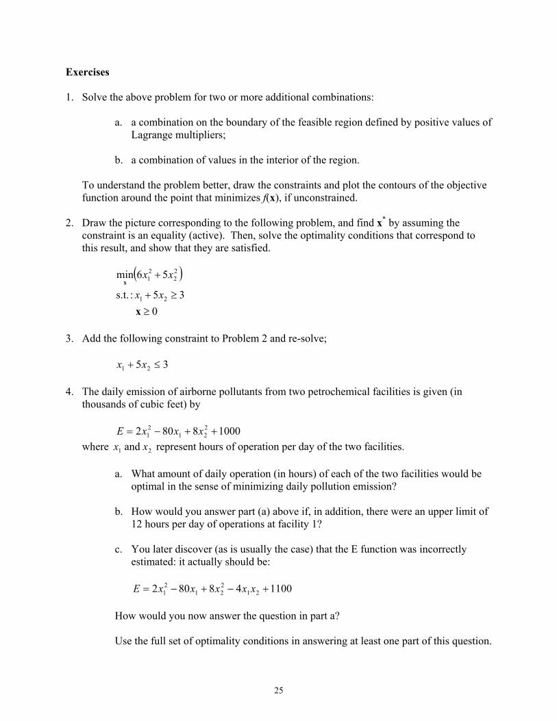
Exercises 1. Solve the above problem for two or more additional combinations:

a. a combination on the boundary of the feasible region defined by positive values of

Lagrange multipliers; b. a combination of values in the interior of the region.

To understand the problem better, draw the constraints and plot the contours of the objective function around the point that minimizes f(x), if unconstrained.

2. Draw the picture corresponding to the following problem, and find x* by assuming the

constraint is an equality (active). Then, solve the optimality conditions that correspond to this result, and show that they are satisfied.

( )

0 35 :s.t.

56min

21

22

21

≥≥+

+

x

x

xx

xx

3. Add the following constraint to Problem 2 and re-solve;

35 21 ≤+ xx

4. The daily emission of airborne pollutants from two petrochemical facilities is given (in

thousands of cubic feet) by

10008802 221

21 ++−= xxxE

where 21 and xx represent hours of operation per day of the two facilities.

a. What amount of daily operation (in hours) of each of the two facilities would be optimal in the sense of minimizing daily pollution emission?

b. How would you answer part (a) above if, in addition, there were an upper limit of

12 hours per day of operations at facility 1?

c. You later discover (as is usually the case) that the E function was incorrectly estimated: it actually should be:

110048802 21

221

21 +−+−= xxxxxE

How would you now answer the question in part a?

Use the full set of optimality conditions in answering at least one part of this question.

26

2. Auto Route Choice Principles We begin our consideration of travel choice models for urban travel forecasting with the problem of how to predict travelers’ choice of route through a roadway network, given the origin and destination of travel. The solution of this route choice problem for road and transit networks, with or without congestion, also establishes a method for determining modal travel costs. With this information, it is then possible to consider models of mode and origin-destination choice, as well as models of choice of residential location. In transportation planning practice, the problem of route choice is traditionally called traffic (or trip) assignment, since origin-destination (O-D) flows were viewed as being mechanically “assigned” to the network. The user-optimal model (UO) of route choice described in these notes is now widely accepted and applied, both by practitioners and researchers, but is still not widely understood, even though a convergent solution algorithm was devised by 1968, based on a formulation published in 1956, and implemented in some computer codes by the mid-1970s. 2.1 User-Optimal Route Choice 2.1.1 Assumptions A British traffic scientist, John Wardrop, proposed the following “criterion” for a network equilibrium in a paper published in 1952:

“The journey times on all routes actually used are equal, and less than those which would be experienced by a single vehicle on any unused route.”

This statement is now known as Wardrop’s first principle for user-optimal (UO) network equilibrium. An alternative statement is that each traveler chooses the shortest route as measured by travel time. The two statements are equivalent because no traveler can find a shorter route if Wardrop’s criterion is met. Beckmann et al (1956) independently stated the same criterion. By used routes, Wardrop meant the routes used from a given origin to a given destination, which in practice are defined in terms of zones. Today, we interpret journey times as generalized costs of travel. In general, routes consist of sequences of links; then, route costs may be defined as the sum of the link costs along the route. Since link costs generally depend on link flows, through the cost-flow function, and each link serves (possibly) many routes, then identifying the route costs and flows which satisfy the above Wardrop condition involves solving the route choice problem for the entire system of zone pairs and the entire network simultaneously. Since link flows have units of vehicles/hour, then the corresponding route flows and O-D flows also have units of vehicles/hour or persons/hour. The resulting route choice model is a steady-state flow or static model in which there is no concept of a traveler moving from an origin to a destination. Rather, there is an O-D flow, with each link of each used route having a corresponding flow. This formulation results in a highly specific concept of “congestion,” in which there are no bottlenecks or traffic jams, only steadily flowing vehicles at speeds determined by the cost-flow performance functions.

27

2.1.2 User-Optimal Formulation In this section, we consider a simple case with a single O-D pair. In Section 2 we shall generalize this case to an entire network. Suppose two nodes A and B are connected by two links, 1 and 2. The fixed O-D flow/hour is d.

Two-Link, Two-Node Example

The travel cost on link 1 is given by ( ),111 fcc = an increasing function of total link flow, where

1f is the flow on link 1; likewise, ( ).222 fcc = Conservation of flow requires that .21 dff =+ If we want the solution such that the link costs are equal at equilibrium, then the user-optimal flows ( )UU ff 21 , can be found graphically as shown above. The user-optimal flows correspond to the intersection of ( )11 fc and ( )22 fc , that is, where the travel costs on the two links are equal.

User Equilibrium Link Travel Times and Flows

0

10

20

30

40

50

60

0 500 1,000 1,500 2,000 2,500 3,000 3,500 4,000

Link 1 Flow (vehicles/hour); Link 2 Flow = 4000 - Link 1 Flow

Link

1 T

rave

l Tim

e (m

inut

es)

0

10

20

30

40

50

60

Link

2 T

rave

l Tim

e (m

inut

es)

Link 2

Link 1

u = 27.1

1,522 2,478

Link 1

Link 2

Node B Node A

d (vehicles/hour) d

( ) ( )( )44111 1000/15.115 ffc +=

( ) ( )( )44222 2000/15.120 ffc +=

( )kfc U +22

( )kfc U −11

k

28

The equilibrium cost is denoted as u; the equilibrium flows are ( ). and 121UUU fdff −= Consider

some other allocation of flows, ( ) ( )kfkf UU +− 21 and . The travel costs at these flows are ( ) ( ).2211 kfckfc UU +<− Thus, this solution does not satisfy Wardrop’s criterion. By an

unspecified process, k vehicles/hour need to switch routes to achieve the user-optimal solution. The above diagram illustrates another attribute of the solution: the area under the link cost-flow functions is minimized at the UO solution. Any other solution, such as ( )kf U −1 , results in a larger area by the amount of the triangle to the right of the vertical line at kf U −1 . This insight suggests an analytical problem formulation: User-Optimal Traffic Assignment Problem (UO TAP)

( )( ) ( ) ( )∫+∫=

21

21 02

01,

minff

ffdxxcdxxcz f (objective function)

dff =+ 21:st (conservation of flow constraint)

0,0 21 ≥≥ ff (non-negativity constraints) A specific form of the travel cost-flow performance function is the BPR function for a link with a zero flow travel time of 0

ac and a nominal capacity of Ca:

⎟⎟

⎠

⎞

⎜⎜

⎝

⎛⎟⎟⎠

⎞⎜⎜⎝

⎛+=

40 15.01

a

aaa C

fcc

The integral of the BPR function is:

( ) ⎟⎟⎠

⎞⎜⎜⎝

⎛⎟⎟⎠

⎞⎜⎜⎝

⎛+=∫ 4

50

0

03.0a

aaa

f

a Cf

fcdxxca

By comparison, the total travel cost on link a is:

( ) ⎟⎟⎠

⎞⎜⎜⎝

⎛⎟⎟⎠

⎞⎜⎜⎝

⎛+≡ 4

50 15.0

a

aaaaa C

ffcfT

2.1.3 Analysis of User-Optimal Conditions Let us proceed to demonstrate analytically that the solution of UO TAP corresponds to the Wardrop condition.

29

( ) ( ) ( ) ( )

( ) ( )

( ) ( ) 01

01

,

222

111

210

20

1

21

≥+−=∂∂

≥+−=∂∂

−+−+= ∫∫

ufcfL

ufcfL

dffudxxcdxxcuLff

f

021 ≥−+=∂∂ dffuL

(if written as an inequality constraint)

( )( ) 0111 =−ufcf

( )( )( )

0,00

21

222

≥≥=−+=−

udffuufcf

0f

In order to take the first derivatives, we need to know that the derivative of an integral with respect to its upper limit is the integrand evaluated at that limit times the partial derivative of the upper limit. More generally,

( ) ( )xzztdyyt

x

z

∂∂⋅=⎟⎟

⎠

⎞⎜⎜⎝

⎛

∂∂∫0

First, we consider the case illustrated by the figure, .0f > In this event, we have:

( )( )( ) ( )UU

U

U

fcfc

ufc

ufc

2211

22

11

so ,

and ,

=

=

=

Hence, at optimality the travel costs are equal; moreover, since u > 0, .21 dff =+ Therefore, Wardrop’s first principle is satisfied. Suppose one of the links is sufficiently low in cost that no flow occurs on the other link. To analyze this situation, we proceed as follows. Assume link 1 is the lower cost link that receives all of the flow. 1. If ( ) ( ) . and , then ,0,0 1221121 dfufcufcff UUUUU =≥==> Note that Wardrop’s first principle is satisfied since the cost of link 2 cannot be less than the cost of link 1; 2. If ( ) ( ) .0 then , 21122 ==> UUU fufcfc In this case, the higher cost of link 2 requires that its flow is 0, according to the above optimality conditions.

30

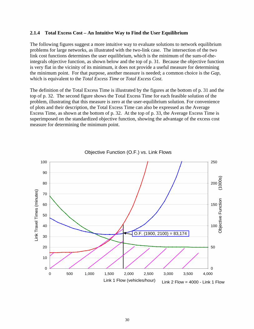
2.1.4 Total Excess Cost – An Intuitive Way to Find the User Equilibrium The following figures suggest a more intuitive way to evaluate solutions to network equilibrium problems for large networks, as illustrated with the two-link case. The intersection of the two link cost functions determines the user equilibrium, which is the minimum of the sum-of-the-integrals objective function, as shown below and the top of p. 31. Because the objective function is very flat in the vicinity of its minimum, it does not provide a useful measure for determining the minimum point. For that purpose, another measure is needed; a common choice is the Gap, which is equivalent to the Total Excess Time or Total Excess Cost. The definition of the Total Excess Time is illustrated by the figures at the bottom of p. 31 and the top of p. 32. The second figure shows the Total Excess Time for each feasible solution of the problem, illustrating that this measure is zero at the user-equilibrium solution. For convenience of plots and their description, the Total Excess Time can also be expressed as the Average Excess Time, as shown at the bottom of p. 32. At the top of p. 33, the Average Excess Time is superimposed on the standardized objective function, showing the advantage of the excess cost measure for determining the minimum point.

Objective Function (O.F.) vs. Link Flows

0

10

20

30

40

50

60

70

80

90

100

0 500 1,000 1,500 2,000 2,500 3,000 3,500 4,000

Link 1 Flow (vehicles/hour)

Link

Tra

vel T

imes

(min

utes

)

0

50

100

150

200

250

(100

0s)

Link 2 Flow = 4000 - Link 1 Flow

Obj

ectiv

e Fu

nctio

n

O.F. (1900, 2100) = 83,174

31

Objective Function and Link Travel Times vs. Flows

0

20

40

60

80

100

120

0 500 1,000 1,500 2,000 2,500 3,000 3,500 4,000

Link 1 Flow (vehcles/hour)

Link

Tra

vel T

imes

(min

utes

)

0

8

16

24

32

40

48

Link 2 Flow = 4000 - Link 1 Flow

Obj

ectiv

e Fu

nctio

n/40

00

User-Optimal Flows = (1,522; 2,478)

Objective Function/4000 = Minimum

Total Excess Time vs. Link Flows

0

10

20

30

40

50

60

70

80

90

100

0 500 1,000 1,500 2,000 2,500 3,000 3,500 4,000

Link 1 Flow (vehicles/hour)

Link

Tra

vel T

imes

(min

utes

)

Total Excess Time at (1900, 2100) = (44.3 - 23.6) x 1900 = 39,300 minutes

Link 2 Flow = 4000 - Link 1 Flow

32

Excess Times and Link Travel Times vs. Flows

0

20

40

60

80

100

120

0 500 1000 1500 2000 2500 3000 3500 4000

Link 1 Flow (vehicles/hour)

Link

Tra

vel T

imes

(min

utes

)

0

50

100

150

200

250

300

(100

0s)

Link 2 Flow = 4000 - Link 1 Flow

Tota

l Exc

ess

Tim

e (m

inut

es)

UO Flows = (1,522; 2,478)

Total Excess Time

Average Excess Time and Link Travel Times vs. Flows

0

20

40

60

80

100

120

0 500 1,000 1,500 2,000 2,500 3,000 3,500 4,000

Link 1 Flow (vehicles/hour)

Link

Tra

vel T

imes

(min

utes

)

0

20

40

60

80

100

120

Link 2 Flow = 4000 - Link 1 Flow

Ave

rage

Exc

ess

Tim

e (m

inut

es)

UO Flows = (1,522; 2,478)

Average Excess Time

33

Average Excess Time and Link Travel Times vs. Flows

0

20

40

60

80

100

120

0 500 1,000 1,500 2,000 2,500 3,000 3,500 4,000

Link 1 Flow (vehicles/hour)

Link

Tra

vel T

imes

(min

utes

)

-40

-20

0

20

40

60

80

Link 2 Flow = 4000 - Link 1 Flow

Ave

rage

Exc

ess

Cos

t and

O.F

./400

0

UO Flows = (1,522; 2,478)

O.F./4000 = MinimumAverage Excess Time = Minimum

2.2 NCP and VIP Formulations To illustrate a more general formulation of the above problem, let’s consider travel cost functions that represent interaction between the two links. As a motivation for the example, consider that at the point where the two links diverge at point A that vehicles choosing Link 2 delay vehicles choosing Link 1. The generalized functions are as follows, where ( )21

T ff=f : ( ) ( )( ) ( ) 2112

4411 0012.00012.01000/15.115 ffcffc +=++=f

( ) ( )( ) ( )22

4422 2000/15.120 fcfc =+=f

If we compute the Hessian for this objective function, we learn that it is not symmetric:

( ) ( ) 00012.01

2

2

1 =∂

∂≠=

∂∂

fc

fc ff

Therefore, the integral of the cost functions is not well-defined. To form the NCP, define:

34

( )( )( )

( )( )( )( ) ,02000/15.120

0012.01000/15.115

21

442

244

1

21

2

1

≥⎥⎥⎥

⎦

⎤

⎢⎢⎢

⎣

⎡

−+−+

−++

=⎥⎥⎥

⎦

⎤

⎢⎢⎢

⎣

⎡

−+−−

=dff

uf

uff

dffucuc

ff

xF and .02

1

≥⎥⎥⎥

⎦

⎤

⎢⎢⎢

⎣

⎡=

uff

x

Solution of the NCP requires that the equilibrium values, ∗x and ∗u satisfy:

( )( )( )( )( )( )( ) 02000/15.120

0012.01000/15.115

2

1

T

21

442

244

1

=⎥⎥⎥

⎦

⎤

⎢⎢⎢

⎣

⎡

•

⎥⎥⎥⎥

⎦

⎤

⎢⎢⎢⎢

⎣

⎡

−+

−+

−++

=⋅∗

∗

∗

∗∗

∗∗

∗∗∗

∗∗

u

f

f

dff

uf

uff

xxF

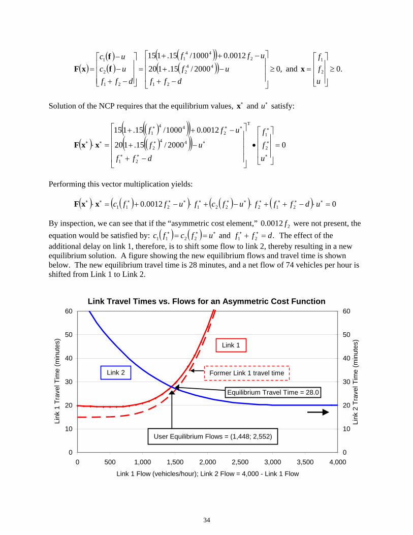
Performing this vector multiplication yields: ( ) ( )( ) ( )( ) ( ) 00012.0 212221211 =⋅−++⋅−+⋅−+=⋅ ∗∗∗∗∗∗∗∗∗∗∗∗ udfffufcfuffcxxF By inspection, we can see that if the “asymmetric cost element,” 20012.0 f were not present, the equation would be satisfied by: ( ) ( ) ∗∗∗ == ufcfc 2211 and .21 dff =+ ∗∗ The effect of the additional delay on link 1, therefore, is to shift some flow to link 2, thereby resulting in a new equilibrium solution. A figure showing the new equilibrium flows and travel time is shown below. The new equilibrium travel time is 28 minutes, and a net flow of 74 vehicles per hour is shifted from Link 1 to Link 2.

Link Travel Times vs. Flows for an Asymmetric Cost Function

0

10

20

30

40

50

60

0 500 1,000 1,500 2,000 2,500 3,000 3,500 4,000

Link 1 Flow (vehicles/hour); Link 2 Flow = 4,000 - Link 1 Flow

Link

1 T

rave

l Tim

e (m

inut

es)

0

10

20

30

40

50

60

Link

2 T

rave

l Tim

e (m

inut

es)

User Equilibrium Flows = (1,448; 2,552)

Equilibrium Travel Time = 28.0

Link 2

Link 1

Former Link 1 travel time

35

Also, note that the performance function for Link 1 is no longer strictly increasing. Next, we consider the VIP formulation of this problem.

( )( )( )( )( )( ) 02000/15.120

0012.01000/15.115

*

*2

*1

2

1

T

*2

*1

*44*2

**2

44*1

≥

⎥⎥⎥⎥

⎦

⎤

⎢⎢⎢⎢

⎣

⎡

⎟⎟⎟⎟

⎠

⎞

⎜⎜⎜⎜

⎝

⎛

−⎟⎟⎟

⎠

⎞

⎜⎜⎜

⎝

⎛•

⎥⎥⎥⎥

⎦

⎤

⎢⎢⎢⎢

⎣

⎡

−+

−+

−++

u

f

f

uff

dff

uf

uff

, 0≥⎟⎟⎟

⎠

⎞

⎜⎜⎜

⎝

⎛

uff

2

1

where uff ,, 21 are nonnegative scalar variables, and d is a constant. Rewriting the VIP as in Section A.5 of the Appendix, we obtain:

( )( )( )( )( )( )

( )( )( )( )( )( ) 02000/15.120

0012.01000/15.115

2000/15.120

0012.01000/15.115

*

*2

*1

T

*2

*1

*44*2

**2

44*1

2

1

T

*2

*1

*44*2

**2

44*1

=⎥⎥⎥

⎦

⎤

⎢⎢⎢

⎣

⎡

•

⎥⎥⎥⎥

⎦

⎤

⎢⎢⎢⎢

⎣

⎡

−+

−+

−++

≥⎥⎥⎥

⎦

⎤

⎢⎢⎢

⎣

⎡•

⎥⎥⎥⎥

⎦

⎤

⎢⎢⎢⎢

⎣

⎡

−+

−+

−++

u

f

f

dff

uf

uff

uff

dff

uf

uff

The right-hand side of the inequality is the same as the equality in the NCP. The VIP states that all nonnegative values of the variables will result in a positive or zero left-hand side. A trivial example is .021 === uff Instead of requiring uff ,, 21 to be nonnegative, suppose we also require 21, ff to satisfy the conservation of flow constraint, .21 dff =+ Then we may remove the third line from the VIP, redefining the constraint space as follows:

( )( )( )( )( )( ) 0

2000/15.120

0012.01000/15.115*

2

*1

2

1

T

*44*2

**2

44*1 ≥

⎥⎥⎦

⎤

⎢⎢⎣

⎡⎟⎟⎠

⎞⎜⎜⎝

⎛−⎟⎟

⎠

⎞⎜⎜⎝

⎛•

⎥⎥⎦

⎤

⎢⎢⎣

⎡

−+

−++

ff

ff

uf

uff, ( ) F, 21 ∈ff

where .;F 21 0f ≥=+= dff The VIP may then be written more compactly as follows, since the terms related to *u are redundant: ( ) ( ) F,*T* ∈≥−⋅ f0fffc A remaining question is whether the function is monotone on the constraint space F . The requirement for the function to be monotone may be stated as: ( ) ( )[ ] ( ) .F,0T ∈∀≥−− gf,gfgcfc

36

To check this condition, the above statement was evaluated for ( )4000g,0 11 ≤≤ f , since

12 000,4 ff −= and .000,4 12 gg −= These values were systematically varied, and plotted as shown below. As can be readily visualized with the plot, the vector product is nonnegative.

Plot of Monotonicity Condition for Existence and Uniqueness

01,000

2,0003,000

4,0000

1,000

2,000

3,0004,000

0.0

0.5

1.0

1.5

2.0

2.5F(

x, y

)*(x

- y)

(milli

ons)

Flow on f Flow on g

2.3 System-Optimal Route Choice Wardrop also stated a second criterion: “The average journey time is a minimum.” Today, we refer to this solution as system-optimal route choice. It has largely been a matter of theoretical analysis, until renewed interest in road pricing has stimulated additional research on this concept. The reason is that achieving system optimal flows requires that the flows be directed along routes in some manner. However, there is a direct interpretation of system-optimal route costs in terms of congestion tolls. We explore this interpretation below. The system-optimal (SO) problem is formulated directly, in contrast to the indirect formulation of the user-optimal (UO) problem, as follows:

( )( )

0f ≥=+

⋅∑dff

ffc aa

aaff

21

,

:s.t.

min21

To solve this problem for the system-optimal flows sf , we proceed as follows, letting v denote the Lagrange multiplier associated with the conservation of flow constraint:

37

( ) ( ) ( )

( ) ( ) ( )

( ) ( ) ( )

( ) ( )

( ) ( )

( )0,

0

0

0

0

01

01

,

21

2

222222

1

111111

21

2

22222

2

1

11111

1

21

≥≥=−+

=⎟⎟⎠

⎞⎜⎜⎝

⎛−

∂∂⋅+

=⎟⎟⎠

⎞⎜⎜⎝

⎛−

∂∂⋅+

≥−+=∂∂

≥+−∂

∂⋅+=

∂∂

≥+−∂

∂⋅+=

∂∂

−+−⋅= ∑

vdffv

vf

fcffcf

vffcffcf

dffvL

vf

fcffcfL

vffcffc

fL

dffvffcvL aa

aa

0f

f

For ease of exposition, define: ( ) ( ) ( )a

aaaaaaa f

fcffcfm

∂∂⋅+≡ . Since ( )aa fm is the derivative of

the total cost of link a, ( ) ),( aaa ffc ⋅ with respect to the flow, af , then ( )aa fm is by definition the Marginal Cost of link a at flow af . To analyze the optimality conditions, consider the case, .0f > Then,

( ) ( ) ( ) where,2211S

aSS ffmvfm == are the system-optimal flows.

Since v > 0 by definition of ( )aa fm , then ( )dff =+ 21 , as required. Alternatively, suppose ( ).0,0 21 => ff Then,

( )( )

dfv

vfm

vfm

S

S

S

=⇒>

≥

=

1

22

11

0

Finally, suppose ( ) ;22 vfm S > then, by the complementary slackness condition on f2, above,

. and 0 12 dff SS == Next consider the value of ( )aa fm based on the BPR function:

( )

( ) ( )⎟⎟⎠

⎞⎜⎜⎝

⎛⎟⎟⎠

⎞⎜⎜⎝

⎛+⎟

⎟⎠

⎞⎜⎜⎝

⎛⎟⎟⎠

⎞⎜⎜⎝

⎛+=⎟

⎟⎠

⎞⎜⎜⎝

⎛⎟⎟⎠

⎞⎜⎜⎝

⎛+=

∂∂

≡

⎟⎟⎠

⎞⎜⎜⎝

⎛⎟⎟⎠

⎞⎜⎜⎝

⎛+=

4

40

4

40

4

40

4

50

60.015.0175.01

15.0

a

aa

a

aa

a

aa

a

aaaa

a

aaaaa

Cfc

Cfc

Cfc

ffTfm

Cf

fcfT

38

From the definition of the Marginal Cost, the derivative of the Total Cost with respect to flow, we may learn that the Marginal Cost is the increase in Total Cost resulting from one additional unit of flow. The first term of the right side of the above equation is the cost incurred by that additional unit of flow. The second term on the right is the additional cost imposed on all af vehicles by the additional unit of flow. The principle of marginal cost road pricing is that each unit of flow (vehicle) should be charged a toll equal to the cost it imposes on all others. This situation may be visualized in the following figure showing the SO flows determined by equating the marginal link costs. By examining the figure carefully, we may observe the differences in generalized cost for the SO and UO solutions. Note for Link 1 that the travel time incurred at the SO flow is less than the UO travel time; however, for Link 2, the UO travel time is greater than the SO time. A toll charged to vehicles on Link 1 equal to ( ) ( )( )SS fcfc 1122 − would adjust the total generalized costs of the two flows to equality at the SO flows. This toll is 4.0 minutes per vehicle.

2.4 Solution Algorithm for the Two-Link Problem based on the Frank-Wolfe Method Next we address the problem of solving for the optimal flows computationally. We first examine this problem for two links. Consider at iteration n that we have a feasible solution ( ) ,, 21

nn ff

where ( )dff nn =+ 21 . For the UO problem, the objective function is: ( ) ( )∑ ∫=a

f

an

na

dxxcz0

f .

v = 61.3 min.

System-Optimal Link Travel Times and Flows

0

10

20

30

40

50

60

70

0 500 1,000 1,500 2,000 2,500 3,000 3,500 4,000

Link 1 Flow (vehicles/hour); Link 2 Flow = 4000 - Link 1 Flow

Use

r and

Mar

gina

l Tra

vel T

ime

(m)

0

10

20

30

40

50

60

70

Use

r and

Mar

gina

l Tra

vel T

ime

(m)

u = 27.1 min.

v = 61.3 min.

478,2

522,1

2

1

=

=U

U

f

f

576,2

424,1

2

1

=

=S

S

f

f

( ) ( )→← 2222 ; fmfc ( )11 fm← ( )11 fc←

39

First, we approximate the objective function at iteration n by its first-order Taylor series,

( ) ( ) ( ) ( ) ( ) ( )( )

( ) ( )C

ggfdcfc

fg

fg

fc

fczzzz

nn

n

n

n

nnnnnn +⎟⎟

⎠

⎞⎜⎜⎝

⎛⋅⎟⎟

⎠

⎞⎜⎜⎝

⎛ −−=⎟

⎟⎠

⎞⎜⎜⎝

⎛

−

−⋅⎟

⎟⎠

⎞⎜⎜⎝

⎛+=−⋅∇+≈

2

1T

1211

22

11

T

22

11

0ffgffg .

Note we substitute ( )nfd 1− for nf2 . Then, we move from the current solution ( )T21

nnn ff=f in the direction of a decrease in ( )nz f pointed by the gradient ( )nz f∇ , called the Search Direction,

to a new solution ( ) .T21nnn gg=g We will refer to nf as the Main Problem solution at iteration n,

and ng as the Subproblem solution at iteration n. This movement is along the tangent line:

( ) ( ) ( ) ( ) ( ) ( ) ( ) ( )

( ) ( ) ( )[ ] ( )nnnn

a

f

a

nnnnnn

a

f

annnn

fgfdcfcdxxc

fgfcfgfcdxxczz

na

na

1112110

222211110

−⋅−−+∑ ∫=

−⋅+−⋅+∑ ∫=−⋅∇+ fgff,

as shown in the next figure. The convex line shows the Objective Function, with a tangent line at (1000, 3000). The Gap is the difference between the Objective Function and the Subproblem solution. In the next figure, the concave line is the Lower Bound on the Objective Function, which equals the Objective Function plus the Gap, whose value is non-positive.

Objective Function and Its Tangent Line

0

100

200

300

400

500

0 500 1,000 1,500 2,000 2,500 3,000 3,500 4,000Flow on Link 1 (vehicles/hour)

Obj

ectiv

e Fu

nctio

n (1

,000

s)

30,750.0

84,562.5 Gap = 53,812.5

84,562.530001000

=⎟⎟⎠

⎞⎜⎜⎝

⎛z

( )fz

( ) ⎟⎠⎞⎜

⎝⎛ −⋅⎟

⎠⎞⎜

⎝⎛∇+⎟

⎠⎞⎜

⎝⎛≈ nnznznz fgffg

40

Objective Function and Its Lower Bound

-200

-100

0

100

200

300

0 5 10 15 20 25 30 35 40

Flow on Link 1 (100s) (vehicles/hour)

Obj

. Fn.

and

Low

er B

ound

(1,0

00s)

The Subproblem can be formulated as follows:

( )

( ) ( ) ( ) ( ) ( )( )

0g

gg

≥

=+

−⋅+−⋅=

n

nn

nnnnnn

dgg

fgfcfgfcz

21

22221111

:st

min

Since ( )nf is fixed, we can solve this problem simply by identifying the lower cost link: ( ) ( )[ ]nn

aa fcfcc 2211ˆ ,min=

Then, we allocate (assign) the total flow d to that link, in order to minimize the total cost. That is, we set .ˆ,0 and ˆ aagdg n

ana ≠== Suppose .1ˆ =a The resulting value of ( )nz g is:

( ) ( ) ( ) ( ) ( )nnnn ffcfdfcz 222111 0−⋅+−⋅=ng Since ( ) ( ) ( ) ( ) ( ) Why?.0 then, 222111112211 ≤⋅−⋅−⋅< nnnnnnn ffcffcdfcfcfc Because ( ) ( ) ( ) ( ) ( ) ( )[ ] .0222112221112111 ≤⋅−=⋅−⋅−+⋅ nnnnnnnnnn ffcfcffcffcfffc

55628430001000

.,z =⎟⎟⎠

⎞⎜⎜⎝

⎛

7503030001000

,LB =⎟⎟⎠

⎞⎜⎜⎝

⎛

41

The value of ( )nz g achieved by the solution (d, 0) is called the Gap, which is the negative of the Total Excess Cost, which as we have seen has an intuitive interpretation. In general, define ( ) ( ) =⋅= ∑ n

aa

naa

n ffcT f total travel cost at the current solution at iteration n

( ) ( ) =∑ ⋅= na

a

naa

n gfcT g total travel cost of the best solution, ng .

Then, ( ) =nz g ( ) ( ) .0≤⋅−⋅ ∑∑ n

aa

naa

na

a

naa ffcgfc

For our two-link example, the Gap and Total Excess Cost calculations are performed as follows:

( )

( ) 5.812,535.562,105250,17000,69 000,31875.35000,125.1701875.35000,425.17 Gap

−=+−=⋅+⋅−⋅+⋅=

Total Excess Cost = ( ) 5.812,53000,325.171875.35 =⋅− Returning to the figure, note that the function lies above the tangent line. Since the objective function is convex, it must lie everywhere above the tangent line at any point. Accordingly, the true optimal solution must be greater than the current objective function value plus the Gap, since the Gap is defined to be .0≤ If the Gap is 0, then the current solution is optimal. The following expression summarizes these points: ( ) ( ) ( ) ( ) ( )n

a

na

naaa

n zfgfczz fff ≤−⋅+≥ ∑∗

For the two-link problem, comparing the cost of the two links tells us whether to shift flow from Link 1 to Link 2 or the opposite. The next question is how much flow to shift, called the Step Size Problem, which is stated as follows:

( )10min

≤≤λ( ) ( )∑ ∫

+

=a

f

a

na

dxxcz1

0λ , where ( ) ( ) n

an

an

ana

na

na gffgff ⋅+⋅−=−⋅+≡+ λλλ 11

We typically solve this problem with a method called bisection search, described as follows: 1. initialize 5.01 =λ ; set a counter k = 1; define .0.00 =λ

2. find ( ) ( ) ( ) ( )=∑ −⋅=∂

∂=′ +

+

a

na

na

naa

n

k fgfczz 11

λλ f slope of the function ( )1+nz f .

a. if ( ) ( ) 2/,0 11 −+ −−=>′ kkkkkz λλλλλ

b. if ( ) ( ) 2/,0 11 −+ −+=<′ kkkkkz λλλλλ

3. stop when ( ) ( ) 0 and ,1 <′<−+ kkk z λελλ at least once; set .1*

+= kλλ

42

The entire solution algorithm may be stated as follows: 1. initialize ;1f set a counter to n = 1; 2. solve the Subproblem for gn;

3. check for convergence: Is the Relative Gap at iteration n, ( ) ε<−≡ n

nnn z

BLBBLB RG f ?

where ( ) ( ) ( )( ) ( )( )nn

nn

nnnn

nn

n zzz ′′

≤′

′′′

≤′+≡−⋅∇+≡ GapmaxmaxBLB ffgff = Best Lower Bound at n

( ) ( )nnn z fgf n −⋅∇=Gap 4. perform line search to obtain *λ and update , to 1+nn ff where ( ) n

an

an

a gff ⋅+⋅−=+ **1 1 λλ 5. check for convergence again with the new value of the objective function ( );1+nz f if not

converged, update the flows according to the above equation, increment n and go to step 2. This solution method is based on a procedure first proposed by M. Frank and P. Wolfe (1956). For this reason, it is generally referred to as the Frank-Wolfe method or algorithm.

λ

174.0=∗λ

Line Search for the Two-Link Example

43

2.5 Braess’s Paradox Several apparent paradoxes of traffic assignment problem have been identified, the most famous being known as Braess’s Paradox. The network shown below (LeBlanc, 1975) exhibits Braess’s Paradox when link (2, 3) is added to the network, which may be stated as follows:

If the route flows are user-optimal, there may exist additions of new links that result in a new User-Optimal solution with a higher total user cost.

link cost functions ( )( )( )( )( ) 4

23

424

413

434

412

0.14.15 3,2

9.0.1854,2

9.0.185 3,1

5.0.40 4,3

5.0.40 2,1

f

f

f

f

f

+

+

+

+

+

Without link (2,3), the UO flows on each link are 3 vehicles/hour. Are these the system-optimal flows as well? Add link (2, 3) and determine the UO and SO flows, route costs and total costs. The solutions for flows ranging from 1 to 12 vehicles per hour are given at the end of this section. References Bar-Gera, H. (2002) Origin-Based Algorithm for the Traffic Assignment Problem, Transportation Science 36, 398-417. Braess, D., A. Nagurney and T. Wakolbinger (2005) On a Paradox of Traffic Planning, Transportation Science 39, 446-450 (translated from the original German published in 1968). Frank, M. and P. Wolfe (1956) An Algorithm for Quadratic Programming, Naval Research Logistics Quarterly 3, 95-110. LeBlanc, L. J. (1975) An Algorithm for the Discrete Network Design Problem, Transportation Science 9, 183-199 Nagurney, A. and D. Boyce (2005) Preface to “On a Paradox of Traffic Planning,” Transportation Science 39, 443-445. Wardrop, J. G. (1952) Some Theoretical Aspects of Road Traffic Research, Proceedings of the Institution of Civil Engineers, Part II 1, 325-378.

1

2

3

4

6 veh./hr. 6 veh./hr.

44

Exercises 1. Consider the following travel cost functions for the two-link problem shown in Section 2.1.2.

( ) ⎟⎟⎠

⎞⎜⎜⎝

⎛⎟⎠⎞

⎜⎝⎛+=

41

11 100015.0115 ffc ( ) ⎟

⎟⎠

⎞⎜⎜⎝

⎛⎟⎠⎞

⎜⎝⎛+=

42

22 200015.0120 ffc

Solve graphically for the solutions of the user-optimal and system-optimal problems for the two-link network with d = 5,000 vehicles/hour. Plot the user travel time functions and the marginal travel time functions in the region of their intersection to yield a good graphical solution. Compute the total travel time for both solutions. How much time is saved by the system-optimal solution? What is the difference in the users’ travel times on the two links at the system-optimal solution? How do these times compare with the users’ travel time for the user-optimal solution? Be careful: compare the users’ travel times, not their marginal times. 2. Apply the Frank-Wolfe algorithm, described in the notes, to solve for the UO flows for the above two-link problem plus the addition of a third link with the following travel cost function:

( ) ⎟⎟⎠

⎞⎜⎜⎝

⎛⎟⎠⎞

⎜⎝⎛+=

43

33 50015.0125 ffc

For your initial solution, take the UO solution that you found for Exercise 1 above. Compute the travel cost for the following links: ( ) ( ) ( ),0,, 32211 cfcfc UU where ( )UU ff 21 , is the solution to Exercise 1. Choose the minimum cost link of these three. Compute the Objective Function, Gap and Lower Bound on the Objective Function using the work sheet given below. Note that the Gap is negative by definition, except at the optimum, where it is zero. Therefore, the Lower Bound should be less than the Objective Function. Perform the line search step to find λ*:

( )10min

≤≤λ( ) ( )∑ ∫

+

=a

f

a

na

dxxcz1

0λ , where ( ) ( ) n

an

an

ana

na

na gffgff ⋅+⋅−=−⋅+≡+ λλλ 11

You may find λ* in one of two ways. One way is to compute ( )λz for several values of λ , and plot ( )λz versus λ , and interpolate the result. If you choose this method, you must find λ sufficiently precisely so that you obtain a decrease in the Objective Function value. For each iteration, you will need to increase the precision of λ from tenths to hundredths to thousandths. The other procedure is to apply the bisection method. In this case, you must continue the method until you obtain a negative value for the slope of the function ( )λz . Tabulate your computations for three iterations of the algorithm following the initial solution. That is, solve for three values of λ*. Plot the objective function and lower bound (y-axis) vs. the iteration number (x-axis).

45

Worksheet for Frank-Wolfe Method, Exercise 2 link 1

af ( )1aa fc ( )∫

1

0

af

a dxxc 1ag ( )11

aa fg − ( ) ( )111aaaa fgfc −⋅

2af

1 2 3 Objective Function = 5,000 Gap = 5,000

Lower Bound = Objective Function + Gap = Relative Gap = Gap/Best Lower Bound =

link 2af ( )2

aa fc ( )∫2

0

af

a dxxc 2ag ( )22

aa fg − ( ) ( )222aaaa fgfc −⋅

3af

1 2 3 Objective Function = 5,000 Gap = 5,000

Lower Bound = Objective Function + Gap = Relative Gap = Gap/ Best Lower Bound =

link 3af ( )3

aa fc ( )∫3

0

af

a dxxc 3ag ( )33

aa fg − ( ) ( )333aaaa fgfc −⋅

4af

1 2 3 Objective Function = 5,000 Gap = 5,000

Lower Bound = Objective Function + Gap = Relative Gap = Gap/ Best Lower Bound =

46

3. This exercise explores the properties of Braess’s Paradox. It also introduces networks with routes of more than one link. a. Solve the Braess’s paradox network shown below for the user-optimal flows. You can do this by applying the Frank-Wolfe method, or you may be able to do it more quickly by trial and error. In the latter case, begin with the network without link (2,3) and solve for the flows by noting the symmetry of the network. If the route costs are equal, then you have found the user-optimal solution, since the solution for this network is unique. link cost functions ( )( )( )( )( ) 4

23

424

413

434

412

0.14.15 3,2

9.0.1854,2

9.0.185 3,1

5.0.40 4,3

5.0.40 2,1

f

f

f

f

f

+

+

+

+

+

b. Add link (2,3) and try moving 1 vehicle/hour to the new lower cost route that includes link (2,3); continue until you find the user-optimal solution, that is the solution in which all three routes have equal travel costs.. Check your answer by comparing it with the result in the Table, at the end of Section 2. Compare the UO route costs for the two solutions, and note that the network with link (2,3) has a higher UO cost. c. Derive the marginal cost functions for the links of this network. Using these marginal cost functions, solve the system-optimal problem for a total flow of 6 vehicles/hour with and without link (2,3). What is the total travel time for each solution? How do these travel times compare with the total travel time for the user-optimal solutions with and without link (2,3)? To solve the SO problem with link (2,3) you will need to consider non-integer link flows. Therefore, you cannot use trial and error, since the number of possibilities is infinite. You can solve this problem using the Frank-Wolfe method, but it is somewhat more involved than the simple three-link problem you solved so far. The reason is that you need to work with link flows and route flows, not just link flows. More formally, you need to work in two different spaces, link flow space and route flow space. The tables below and on the next pages are provided to facilitate your work. Begin with the route table and enter the solution without link (2, 3). Compute the link costs in the link table, and then determine the route costs. d. Now re-solve for the UO and SO flows with a total flow of 12 vehicles/hour entering and leaving the network. For this problem, start with the solution without link (2,3), and then apply

1

2

3

4

6 veh./hr. 6 veh./hr.

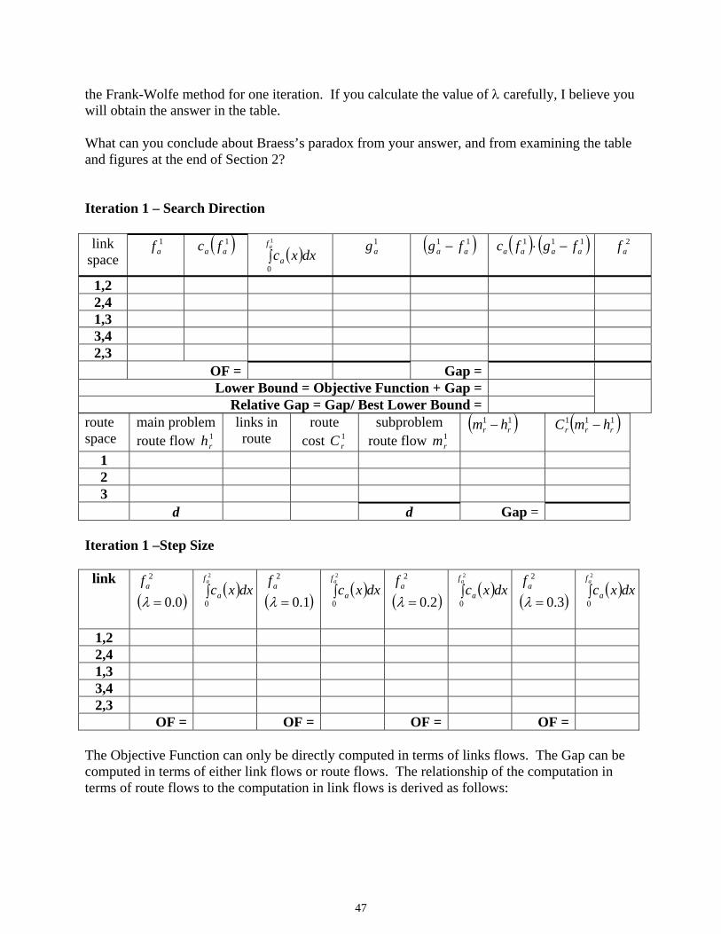
47

the Frank-Wolfe method for one iteration. If you calculate the value of λ carefully, I believe you will obtain the answer in the table. What can you conclude about Braess’s paradox from your answer, and from examining the table and figures at the end of Section 2? Iteration 1 – Search Direction

route space

main problem route flow 1

rh links in route

route cost 1

rC subproblem

route flow 1rm

( )11rr hm − ( )111

rrr hmC −

1 2 3

d d Gap = Iteration 1 –Step Size

link

( )0.0

2

=λaf

( )∫2

0

af

a dxxc

( )1.0

2

=λaf

( )∫2

0

af

a dxxc

( )2.0

2

=λaf

( )∫2

0

af

a dxxc

( )3.0

2

=λaf

( )∫2

0

af

a dxxc

1,2 2,4 1,3 3,4 2,3

OF = OF = OF = OF = The Objective Function can only be directly computed in terms of links flows. The Gap can be computed in terms of either link flows or route flows. The relationship of the computation in terms of route flows to the computation in link flows is derived as follows:

link space

1af ( )1

aa fc ( )∫1

0

af

a dxxc 1ag ( )11

aa fg − ( ) ( )111aaaa fgfc −⋅

2af

1,2 2,4 1,3 3,4 2,3

OF = Gap = Lower Bound = Objective Function + Gap =

Relative Gap = Gap/ Best Lower Bound =

48

( ) ( ) ( ) ( ) ( )

( ) ( ) ( )nr

nr

rr

nr

nr

ar

r a

naa

a r

nr

nr

ar

naa

a r

ar

nr

r

ar

nr

naa

a

na

na

naa

hmChmfc

hmfchmfcfgfc

−⋅∑=−⋅∑∑=

∑ ∑ −⋅=∑ ⎟⎠⎞⎜

⎝⎛ ∑−∑⋅=∑ −⋅

δ

δδδ

where a

rδ = 1 if link a belongs to route r, and 0 otherwise, and nrm = the Subproblem route flow.

So, if you have the route costs and route flows for the current Main Problem solution, you can compute the gap using the first table above. Iteration 2 – Search Direction

route space

main problem route flow 2

rh links in route

route cost 2

rC subproblem

route flow 2rm

( )22rr hm − ( )222

rrr hmC −

1 2 3

d d Gap = Iteration 2 –Step Size

link

( )0.0

3

=λaf

( )∫3

0

af

a dxxc

( )=λ

3af

( )∫3

0

af

a dxxc

( )=λ

3af

( )∫3

0

af

a dxxc

( )=λ

3af

( )∫3

0

af

a dxxc

1,2 2,4 1,3 3,4 2,3

OF = OF = OF = OF =

link space

2af ( )2

aa fc ( )∫2

0

af

a dxxc 2ag ( )22

aa fg − ( ) ( )222aaaa fgfc −⋅

3af

1,2 2,4 1,3 3,4 2,3

OF = Gap = Lower Bound = Objective Function + Gap =

Relative Gap = Gap/ Best Lower Bound =

49

Iteration 3 – Search Direction route space

main problem route flow 3

rh links in route

route cost 3

rC subproblem

route flow 3rm

( )33rr hm − ( )333

rrr hmC −

1 2 3

d d Gap =

Iteration 3 –Step Size

link

( )0.0

4

=λaf

( )∫4

0

af

a dxxc

( )=λ

4af

( )∫4

0

af

a dxxc

( )=λ

4af

( )∫4

0

af

a dxxc

( )=λ

4af

( )∫4

0

af

a dxxc

1,2 2,4 1,3 3,4 2,3

OF = OF = OF = OF =

link space

3af ( )3

aa fc ( )∫3

0

af

a dxxc 3ag ( )33

aa fg − ( ) ( )333aaaa fgfc −⋅

4af

1,2 2,4 1,3 3,4 2,3

OF = = Gap = Lower Bound = Objective Function + Gap =

Relative Gap = Gap/ Best Lower Bound =

50

Example of Braess’s Paradox with Original Capacities from LeBlanc (1975) TS, 186-188. Flows computed with the Origin-Based Traffic Assignment Algorithm of Bar-Gera (2002).

total flow: with link 2 - 3 without link 2 - 3 1 to 4

1 From To Volume Link Cost Total Cost From To Volume Link Cost Total Cost 1 2 1 40.5 40.5 1 2 0.5 40.0313 20.02 1 3 0 185.0 0 1 3 0.5 185.0563 92.53 2 4 0 185.0 0 2 4 0.5 185.0563 92.53 2 3 1 16.4 16.4 2 3 0 ∞ 0 3 4 1 40.5 40.5 3 4 0.5 40.0313 20.02 total cost 97.4 225.09 mean cost 97.4 225.092 From To Volume Link Cost Total Cost From To Volume Link Cost Total Cost 1 2 2 48.0 96.0 1 2 1 40.5 40.5 1 3 0 185.0 0 1 3 1 185.9 185.9 2 4 0 185.0 0 2 4 1 185.9 185.9 2 3 2 31.4 62.8 2 3 0 ∞ 0 3 4 2 48.0 96.0 3 4 1 40.5 40.5 total cost 254.8 452.8 mean cost 127.4 226.43 From To Volume Link Cost Total Cost From To Volume Link Cost Total Cost 1 2 3 80.5 241.5 1 2 1.5 42.5313 63.80 1 3 0 185.0 0 1 3 1.5 189.5563 284.33 2 4 0 185.0 0 2 4 1.5 189.5563 284.33 2 3 3 96.4 289.2 2 3 0 ∞ 0 3 4 3 80.5 241.5 3 4 1.5 42.5313 63.80 total cost 772.2 696.26 mean cost 257.4 232.094 From To Volume Link Cost Total Cost From To Volume Link Cost Total Cost 1 2 3.4056 107.2579 365.28 1 2 2 48.0 96.0 1 3 0.5944 185.1123 110.03 1 3 2 199.4 398.8 2 4 0.5944 185.1123 110.03 2 4 2 199.4 398.8 2 3 2.8112 77.8545 218.86 2 3 0 ∞ 0 3 4 3.4056 107.2579 365.28 3 4 2 48.0 96.0 total cost 1169.48 989.6 mean cost 292.37 247.4 5 From To Volume Link Cost Total Cost From To Volume Link Cost Total Cost 1 2 3.7236 136.1225 506.87 1 2 2.5 59.5313 148.83 1 3 1.2764 187.3888 239.18 1 3 2.5 220.1563 550.39 2 4 1.2764 187.3888 239.18 2 4 2.5 220.1563 550.39 2 3 2.4472 51.2663 125.46 2 3 0 ∞ 0 3 4 3.7236 136.1225 506.87 3 4 2.5 59.5313 148.83 total cost 1617.56 1398.43 mean cost 323.51 279.69

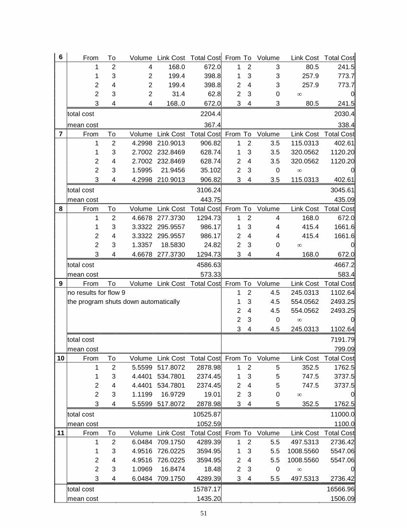
51

6 From To Volume Link Cost Total Cost From To Volume Link Cost Total Cost 1 2 4 168.0 672.0 1 2 3 80.5 241.5 1 3 2 199.4 398.8 1 3 3 257.9 773.7 2 4 2 199.4 398.8 2 4 3 257.9 773.7 2 3 2 31.4 62.8 2 3 0 ∞ 0 3 4 4 168..0 672.0 3 4 3 80.5 241.5 total cost 2204.4 2030.4 mean cost 367.4 338.47 From To Volume Link Cost Total Cost From To Volume Link Cost Total Cost 1 2 4.2998 210.9013 906.82 1 2 3.5 115.0313 402.61 1 3 2.7002 232.8469 628.74 1 3 3.5 320.0562 1120.20 2 4 2.7002 232.8469 628.74 2 4 3.5 320.0562 1120.20 2 3 1.5995 21.9456 35.102 2 3 0 ∞ 0 3 4 4.2998 210.9013 906.82 3 4 3.5 115.0313 402.61 total cost 3106.24 3045.61 mean cost 443.75 435.098 From To Volume Link Cost Total Cost From To Volume Link Cost Total Cost 1 2 4.6678 277.3730 1294.73 1 2 4 168.0 672.0 1 3 3.3322 295.9557 986.17 1 3 4 415.4 1661.6 2 4 3.3322 295.9557 986.17 2 4 4 415.4 1661.6 2 3 1.3357 18.5830 24.82 2 3 0 ∞ 0 3 4 4.6678 277.3730 1294.73 3 4 4 168.0 672.0 total cost 4586.63 4667.2 mean cost 573.33 583.49 From To Volume Link Cost Total Cost From To Volume Link Cost Total Cost no results for flow 9 1 2 4.5 245.0313 1102.64 the program shuts down automatically 1 3 4.5 554.0562 2493.25 2 4 4.5 554.0562 2493.25 2 3 0 ∞ 0 3 4 4.5 245.0313 1102.64 total cost 7191.79 mean cost 799.09

10 From To Volume Link Cost Total Cost From To Volume Link Cost Total Cost 1 2 5.5599 517.8072 2878.98 1 2 5 352.5 1762.5 1 3 4.4401 534.7801 2374.45 1 3 5 747.5 3737.5 2 4 4.4401 534.7801 2374.45 2 4 5 747.5 3737.5 2 3 1.1199 16.9729 19.01 2 3 0 ∞ 0 3 4 5.5599 517.8072 2878.98 3 4 5 352.5 1762.5 total cost 10525.87 11000.0 mean cost 1052.59 1100.0

11 From To Volume Link Cost Total Cost From To Volume Link Cost Total Cost 1 2 6.0484 709.1750 4289.39 1 2 5.5 497.5313 2736.42 1 3 4.9516 726.0225 3594.95 1 3 5.5 1008.5560 5547.06 2 4 4.9516 726.0225 3594.95 2 4 5.5 1008.5560 5547.06 2 3 1.0969 16.8474 18.48 2 3 0 ∞ 0 3 4 6.0484 709.1750 4289.39 3 4 5.5 497.5313 2736.42 total cost 15787.17 16566.96 mean cost 1435.20 1506.09

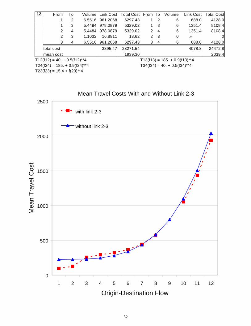
52

12 From To Volume Link Cost Total Cost From To Volume Link Cost Total Cost 1 2 6.5516 961.2068 6297.43 1 2 6 688.0 4128.0 1 3 5.4484 978.0879 5329.02 1 3 6 1351.4 8108.4 2 4 5.4484 978.0879 5329.02 2 4 6 1351.4 8108.4 2 3 1.1032 16.8811 18.62 2 3 0 ∞ 0 3 4 6.5516 961.2068 6297.43 3 4 6 688.0 4128.0 total cost 3895.47 23271.54 4078.8 24472.8 mean cost 1939.30 2039.4

T12(f12) = 40. + 0.5(f12)**4 T13(f13) = 185. + 0.9(f13)**4 T24(f24) = 185. + 0.9(f24)**4 T34(f34) = 40. + 0.5(f34)**4 T23(f23) = 15.4 + f(23)**4

Mean Travel Costs With and Without Link 2-3

0

500

1000

1500

2000

2500

1 2 3 4 5 6 7 8 9 10 11 12

Origin-Destination Flow

Mea

n Tr

avel

Cos

t

with link 2-3

without link 2-3

53

Mean Travel Cost Difference:Without Link 2-3 Less With Link 2-3

-60

-20

20

60

100

140

1 2 3 4 5 6 7 8 9 10 11 12

Origin-Destination Flow

Mea

n Tr

avel

Cos

t Diff

eren

ce:

with

out l

ink

2-3

less

with

link

2-3

0

54

3. Road and Transit Network Route Choice 3.1 Network Concepts and Shortest Route Algorithms One of the first uses of computers for solving large-scale planning and engineering problems was for the shortest route problem for urban transportation networks of realistic size and detail. This capability enabled transportation planners to estimate origin-destination flows and link flows for alternative network proposals for the first time. Thus, the shortest route problem was used as a key portion of a heuristic for the traffic assignment problem. This application was first made in 1958 using an IBM 704 computer with 32,000 words of memory. 3.1.1 Network Concepts and Definitions A transportation network as used in this problem is a mathematical or abstract representation of a system of roadways or transit lines. The treatment here has road systems in mind; these concepts can be extended to include transit systems. node a location on a network that is the intersection of two or more links link (or arc) a pair of nodes which are connected directly, and a number or function

representing the generalized cost of travel between the two nodes; usually links are directed, or one-way, which means they represent the traffic moving from the tail node (a-node) to the head node (b-node).

network a set of nodes and a set of links defined on the nodes centroid a node representing a zone, or small geographic area, through which flows

enter and leave the network

route sequence of directed links connecting an origin centroid with a destination centroid (also called a path)

tree a network in which there is one and only one route from the node R to every other node, and no circuits; that is, it is not possible to return to R after leaving it; node R is called the origin or root of the tree.

shortest route tree a tree in which every route is the shortest route from R to each node (also

called a minimum cost tree or a skim tree). 3.1.2 Properties of Trees 1. The number of links in a tree is n-1, where n is the number of nodes. 2. The shortest route from R to a node k includes as subroutes the shortest routes from R

to the intermediate nodes along the route. A predecessor or back node is the first node back towards the origin node R from a given node i.

55

3. The shortest route tree of origin R can be completely described by two arrays of length n:

a. a predecessor node array, P(I), giving the predecessor node of I, where, P(R) = 0. b. a travel cost array, C(I), giving the minimum cost from R to I.

3.1.3 Shortest Route Problem The shortest route (or path) problem for a centroid R is to find the shortest route tree rooted at origin R. The shortest route problem for N centroids is to find all N shortest route trees. This problem can also be solved for all nodes of the network. There are two basic approaches to solving the shortest route problem: 1. tree-building algorithms which find the shortest route tree for a given origin node using a

labeling technique; 2. matrix methods that find the shortest routes from every node to every other node in one well-

defined sequence of matrix operations. Although the matrix method concept of finding all shortest routes at once seems appealing, it is not practical for large networks because a matrix of size (n times n) can be very large; also, it finds the shortest routes between all pairs of nodes, not just between all centroids. For the purpose of traffic assignment only the latter is needed. Typically, the ratio of nodes to centroids is about 5:1. Tree building algorithms consist of two basic types: 1. label setting methods: destination nodes are permanently labeled with their shortest route

costs in order of increasing cost from the origin; 2. label correcting method: destinations are initially labeled with their route costs as they are

encountered, and then revised if a shorter route is identified. The disadvantage of type 1 is that the minimum value of an array of candidate link costs must be found repeatedly. The disadvantage of type 2 is that route costs must be updated when a shorter route is found. These types of algorithms are based on papers by Dijkstra and others, and Moore respectively. Many improvements have been found in these algorithms since they were proposed in the late 1950's. The best algorithm for a given application depends on the specific network characteristics and the computer on which it is solved. Nowadays, research on shortest path algorithms and computer codes lies more in the field of computer science than in the field of transportation science and engineering. Students transportation science should have a basic understanding of how such algorithms work; however, in my personal view, they should not consider the creation of new codes, or the refinement of existing ones, to be an appropriate research topic. Literature reviews on shortest route algorithms may be found in three papers listed at the end of Section 3.

56

3.1.4 The Dijkstra Algorithm Assume that all link costs cij are nonnegative. Let Cj be the cost from the origin node to any node j. 1. Label the origin node as node 0 with Cj = 0. 2. Let 1, 2, 3, … k be labels at increasing cost from node 0; that is, ....321 kCCCC <<<< 3. To label next node, given that k-1 nodes are labeled,

a. find node j that is connected to the tree of labeled nodes by at least one link from some labeled node i;

b. form ( )iji cC + for each candidate defined in 3a, where ijc is the cost of the link from node i to node j;

c. find ( )ijiijj cCc += min* and label the end node k; designate node i as the predecessor node

of k; in case of ties, label one node k and the other k+1. 4. Repeat step (3) until all nodes have been labeled, or until all centroids are reached. 3.2 Auto Route Choice on a Network with Fixed OD Flows Next, we generalize the route choice formulation for the two-link problem in Section 2 to a general network. To solve the problem, we will use the capability described above to find shortest routes through the network. 3.2.1 UO-TAP on a Network

( )( ) ( )

∑ ∈∑≡

∈∈∈≥

∈∈=∑

∑ ∫=

∈

∈

pq Rr

arra

pqr

pqRr

r

a

f

a

Aahf

QqPpRrh

QqPpdh

dxxcz

pq

pq

a

, where

;,0

;,:st

min

,

0

δ

hh

where =pqd fixed flow from zone p to zone q (vehicles/hour) =rh flow on route r, a route from zone p to zone q that belongs to the set of routes pqR connecting zone p to zone q ,1=a

rδ if link a belongs to route r from zone p to zone q, and 0 otherwise ( ) =aa fc generalized travel cost function for link a, depending only on fa, the flow on link a =QP, sets of origin and destination zones, respectively Note that the unknown variables are the route flows (hr), and that the link flows (fa) are defined in terms of the route flows. The link-route correspondence array ( )a

rδ is assumed to be known.

57

However, it is determined only as needed by use of the shortest route algorithm described above for problems of any size. The optimality conditions for UO-TAP are determined as follows. Define the Lagrangean function:

( ) ( ) ∑ ∑∑ ∫ ⎟⎟⎠

⎞⎜⎜⎝

⎛−−=

∈pq Rrpqrpq

a

f

apq

a

dhudxxc,L0

uh

Consider the derivative of the objective function with respect to the route flow hr, the general

unknown variable: ( ) ( ) ( )∑ ⋅=∂∂⋅

∂∂

=∂∂

a

araa

r

a

ar

fchf

fz

hz δhh

The optimality conditions may then be stated as follows:

( ) ( )

( ) ( )

0u0h ≥≥

∈∈=⎟⎟⎠

⎞⎜⎜⎝

⎛∑ −⋅

∈∈≥⎟⎟⎠

⎞⎜⎜⎝

⎛∑ −

∈∈∈=⎟⎠⎞⎜

⎝⎛ +−∑ ⋅⋅

∈∈∈≥+−∑ ⋅

∈

∈

,

,,0

,,0

,,,01

,,,01

QqPpdhu

QqPpdh

QqPpRrufch

QqPpRrufc

pq

pq

Rrpqrpq

Rrpqr

pqpqa

araar

pqpqa

araa

δ

δ

These conditions may be interpreted in the following way for OD pair pq:

1. assume then,;0>rh ( ) ( ) ( ) pqa

araarpq

a

araa ufcCufc =⋅≡=⎟

⎠⎞

⎜⎝⎛ +−⋅ ∑∑ δδ or ,01 ;

2. assume ( ) ( ) ;or ,01 then,;0 pqrpqa

araar uCufch ≥≥⎟

⎠⎞

⎜⎝⎛ +−⋅= ′′′ ∑ δ

3. assume .0 then; => ′′′′ rpqr huC Hence, every used route connecting zone p to zone q has the equal generalized travel cost upq, and no unused route has a lower travel cost. Therefore, Wardrop’s first principle is satisfied for this formulation. A similar formulation may be formulated for the System-Optimal problem by replacing ca(fa) by the marginal cost function ma (fa). If the generalized cost functions are strictly increasing with link flow, then the solution is unique in the link flows; however, it is not unique in the route flows. The reason is that the link flows are a linear function of the route flows; therefore, the objective function is not strictly convex in the route flows.

58

3.2.2 Nonlinear Complementarity and Variational Inequality Formulations of UO-TAP Following the procedure described in Appendix A.5, we can formulate the NCP corresponding to the above problem as follows:

( )( )

0yF ≥⎥⎥⎥

⎦

⎤

⎢⎢⎢

⎣

⎡

∈∈∑ −

∈∈∈−∑ ⋅=

∈QqPpdh

QqPpRrufc

pqRrpqr

pqpqa

araa

,

,,δ 0y ≥

⎥⎥⎦

⎤

⎢⎢⎣

⎡

∈∈

∈∈∈=

QqPpu

QqPpRrh

pq

pqr

,

,,

( )( )

( )

( )

( ) ( ) ( ) . where,0

0,

,,,

,,

, ,

, ,,,

,,

T

T

∑ ⋅≡=⎥⎦

⎤⎢⎣

⎡∑ ∑ ⋅−∑ ⋅=

⎥⎦

⎤⎢⎣

⎡∑ ∑ ⋅−∑⋅+∑ ∑⋅−∑ ∑ ⋅=

⎥⎦

⎤⎢⎣

⎡∑ ⎟⎟

⎠

⎞⎜⎜⎝

⎛∑ −⋅+∑ ∑ ⎟

⎠⎞⎜

⎝⎛ −∑ ⋅⋅=

=⎥⎥⎦

⎤

⎢⎢⎣

⎡

∈∈

∈∈∈⋅

⎥⎥⎥

⎦

⎤

⎢⎢⎢

⎣

⎡

∈∈∑ −

∈∈∈−∑ ⋅=⋅

∈∈ ∈∈∈

∈∈ ∈∈∈∈∈ ∈∈∈ ∈

∈∈ ∈∈∈ ∈

∈

a

araar

QqPp QqPppqpq

Rrrr

pqQqPp QqPp

pqRr

rpqQqPp Rr

rpqQqPp Rr

rr

QqPp Rrpqrpq

QqPp Rrpq

a

araar

pq

pqr

Rrpqr

pqpqa

araa

fcCudCh

udhuhuCh

dhuufch

QqPpu

QqPpRrhQqPpdh

QqPpRrufc

pq

pqpqpq

pqpq

pq

δ

δ

δ

ff

f

yyF

This requirement states at equilibrium that the total travel costs determined in terms of route costs and route flows must equal the total travel costs stated in terms of the fixed OD flows and the user-optimal OD costs. Note that the asterisks denoting that all flows are equilibrium are omitted in order to simplify the expression. The equivalence of total route-based costs and total OD-based costs is a basic property of the equilibrium solution, which holds for each OD pair. The equivalent VIP may be stated as follows:

( ) ( )( ) 0

,

,,

,

,,T

≥⎥⎥⎦

⎤

⎢⎢⎣

⎡

∈∈−

∈∈∈−⋅

⎥⎥⎥

⎦

⎤

⎢⎢⎢

⎣

⎡

∈∈∑ −

∈∈∈−∑ ⋅

∗

∗

∈

∗

∗∗

QqPpuu

QqPpRrhh

QqPpdh

QqPpRrufc

pqpq

pqrr

Rrpqr

pqpqa

araa

pq

δ,

0u0h

≥≥

.

By moving the conservation flow constraints into the definition of the constraint space, we may simplify the formulation as follows:

( ) ( )[ ] 0,,,,T

≥∈∈∈−⋅⎥⎦⎤

⎢⎣⎡ ∈∈∈∑ ⋅ ∗∗ QqPpRrhhQqPpRrfc pqrrpq

a

araa δ , or

( ) ( ) 0≥−⋅∑ ∑ ∗

∈

∗rr

pq Rrr hhC

pq

f , R;,,H n

Rrpqrr QqPpdhh

pq+

∈

∗ ∈∈∑ −=∈ , which is equivalent to:

( ) ( ) ;,;,,F,0* 0h ≥∑ ∈∑≡∈∈∑ −=∈≥∑ −⋅∈∈

∗

pq Rr

arra

Rrpqra

aaaaa AahfQqPpdhffffc

pqpq

δ

59

3.3 Solution Algorithm for UO-TAP based on the Frank-Wolfe Method A solution algorithm for UO-TAP for the case of a general network with separable link costs

( )( )aaa fcc ≡ may be readily defined as a generalization of the algorithm for the two-link problem described in Section 2. This algorithm is generally known as the Frank-Wolfe algorithm or method; it is known to converge relatively slowly after the first few iterations. The algorithm may be stated as follows: 1. initialize ;nf set a counter to n = 1; a typical method is to perform an all-or-nothing

assignment to the zero-flow link generalized costs; see the following subsection for a definition of all-or-nothing assignment;

2. solve the Subproblem for gn, the Subproblem link flows, as described below;

3. check for convergence of the Relative Gap at iteration n: ( ) ? RG Is ε<−≡ n

nnn

BLBBLBz f

where ( ) ( ) ( )( ) ( )( )( )nn

nn

nnnn

nn

n zzzBLB ′′

≤′

′′′′

≤′+=−⋅∇+≡ Gapmaxmax ffgff

( ) ( )nnnn z fgf −⋅∇≡Gap 4. perform a line search, as described below, to obtain nλ and set ( ) nnnnn gff ⋅+⋅−=+ λλ11 5. check for convergence again with the new value of the objective function ( );1+nz f if not

converged, increment n to n+1, and go to step 2. Solution of the Subproblem (Step 2) The Subproblem is found by approximating the objective function at solution nf , as follows:

( ) ( ) ( ) ( ) ( ) constant0

+⋅∑=−⋅∑+∑ ∫≈ na

a

naa

na

na

a

naa

a

f

an gfcfgfcdxxcz

na

g

To solve the Subproblem subject to the conservation of flow constraints, we formulate the following problem, where h is now the subproblem route flow:

( )( )

∑ ∈∑≡

≥

∈∈=∑

⋅∑

∈

∈

pq Rr

arra

pqRr

r

na

a

naa

Aahg

QqPpdh

gfc

pq

pq

,ˆ where

ˆ

;,ˆ:st

min

δ

0h

g

60

Since ( )naa fc is temporarily fixed at nf , this is a linear programming problem in .ng The above

problem in the space of link flows may be transformed to the space of route flows, as follows: ( ) ( ) ( ) ( )∑ ∑ ⋅=⋅∑∑ ∑ ⋅=∑ ∑⋅∑=⋅∑

∈∈∈ pq Rrr

nr

ar

a

naa

pq Rrr

pq Rr

arr

a

naa

na

a

naa

pqpqpq

hCfchhfcgfc ˆˆˆ fδδ

where ( ) ( ) a

ra

naa

nr fcC δ⋅≡ ∑f is the travel cost on route r with flows nf . This transformation is

carried out by rearranging the terms in the above equation and refactoring, may be shown by writing out the equation in detail. Since ( )n

rC f is a constant, the problem, ( )

( )∑ ∑ ⋅∈≥ pq Rr

rn

rpq

hC ˆminˆ

f0h

may be solved by identifying the minimum cost route from p to q, and placing all of the OD flow

pqd on that route. Such a solution is traditionally called an all-or-nothing solution. A more meaningful name would be minimum cost route solution. The solution is readily found by applying the shortest route algorithm to the network with link costs ( )( )n

aa fc and placing the entire OD flow on each minimum cost route. Summing these route flows to link flows yields the Subproblem solution ng . Solution of the Line Search (Step 4)

The line search is defined as: ( )

( ) ( )∑ ∫+

=≤≤ a

f

a

na

ndxxcz

1

010min λλ

,

where ( ) ( ) n

ann

ann

ana

nna

na gffgff ⋅+⋅−=−⋅+=+ λλλ 11

This problem consists of the minimization of a nonlinear function with respect to a scalar. Such problems may be readily solved by applying a line search technique, such as bisection search. To apply this technique, we require the partial derivative of the objective function with respect to the unknown variable nλ , which may be stated as follows:

( ) ( ) ( )na

na

a

naa fgfcz

−⋅=∂∂

∑ +1

λλ

Using this result, the bisection search proceeds as follows: 1. initialize 5.01 =λ ; set k = 1, and .0.10 =λ

61

2. find ( ) ( ) ( )∑ −⋅=′ +

a

na

na

naak fgfcz 1λ = slope of the function ( )λz .

a. if ( ) ( ) 2/,0 11 −+ −−=>′ kkkkkz λλλλλ b. if ( ) ( ) 2/,0 11 −+ −+=<′ kkkkkz λλλλλ

3. stop when ( ) ( ) 0 and ,1 <′<− − kkk z λελλ at least once. The last requirement assures that the chosen value of λ results in a decrease in the Main Problem objective function. If this requirement were not fulfilled, the chosen value of λ would lie to the right of its minimum value, and could correspond to a higher value of the Main Problem objective function than the present value. Draw the curve of the Main Problem objective function vs. λ to see this point. In computational experiments for a large network, it was shown that ε can be as large as 0.25 without increasing the overall solution time significantly. Selecting a value as large as 0.25 may substantially reduce the computational effort of the line search. 3.4 Origin-Based Traffic Assignment Algorithm 3.4.1 Overview The algorithm described in this section was formulated, implemented and extensively tested on large networks by Hillel Bar-Gera (1999, 2002), starting with his Ph.D. thesis, and continuing since that time. This section is intended to give a short, relatively nonmathematical overview of the algorithm. The Frank-Wolfe algorithm may be characterized as being link-based, since the solution variables are link flows. Another type of algorithms is route-based, in that each route flow is a solution variable. Route-based algorithms were proposed by Bothner and Lutter (1982) and Larson and Patriksson (1992); the former is the basis for one practitioner software system. The concept of the Origin-Based Assignment (OBA) algorithm is to define the solution variables in an intermediate way between links and routes. In this way the algorithm seeks to solve larger networks efficiently than can be solved by either of the two approaches. For examples of comparisons of solutions, see Bar-Gera (2002). The main solution variables in this algorithm are origin-based approach proportions, αpa, for every origin p and every link a, such that for every origin p and node i the sum of origin-based approach proportions over all links ending at node i is equal to one. Using origin-based approach proportions, route proportions are determined by the product of approach proportions of all the links along the route, that is ∏

⊆

=ra

papqr αγ . Route flows are determined by the product

of OD flow and route proportion, that is pqrpqpqr dh γ⋅= . It can be shown (Bar-Gera, 2002, eq. 14) that if link a goes from node i to node j, and if the total flow from origin p to node j is gpj, then the total flow from origin p that arrives at node j through link a is pjpapa gf ⋅= α ; in that respect αpa is indeed the proportion of flow on approach a to node j for origin p, as implied from the name of these variables.

62

The representation of the solution by origin-based approach proportions allows storing a complete description of the route flows very efficiently. The efficiency of the representation is further enhanced using the fact that at most nodes one link receives approach proportion value of one, while the value of all other links ending at the same node is zero. The availability of route flows can be useful for solution analysis. It is also useful in searching for the equilibrium solution, which is a major difference from many alternative solution procedures, including the Frank-Wolfe algorithm, which store only total link flows during the iterative process. A key point in this algorithm is that for every origin an a-cyclic restricting subnetwork is chosen, Ap, such that for origin p approach proportions of links that are not included in Ap are restricted to 0. Using the equation for route proportions it can be seen that under these restrictions, for every origin, only routes that are limited to the links in its restricted subnetwork can be used. In particular, since Ap is a-cyclic, meaning that it does not contain a directed cycle of links, any cyclic route must contain at least one link that does not belong to Ap, and hence the flow along any cyclic route must be zero. It is important to note that the restriction to a-cyclic subnetworks does exclude many solutions that do not use cyclic routes, which are usually considered legitimate. It can be shown (for example, Bar-Gera, 2002; Lemma 3) that there is always an equilibrium solution that is a-cyclic by origin. Therefore, this restriction does not prevent the algorithm from converging to the true equilibrium solution. The restriction to solutions that are a-cyclic by origin has several important advantages. First, the simple route flow interpretation presented above is, in fact, only valid for solutions that are a-cyclic by origin. Second, a-cyclic subnetworks allow a definition of a topological order of the nodes, which is an origin-specific ordering of the nodes, such that every link in the restricting subnetwork goes from a node of lower topological order to a node of higher topological order. Most computations in the proposed algorithm are done in a single pass over the nodes, either in ascending or descending topological order. The time required by such computations is a linear function of the number of links in the network. This computational efficiency is the main reason for restricting to a-cyclic solutions. In solving the traffic assignment problem, the algorithm starts with trees of minimum cost routes as restricting subnetworks, leading to an all-or-nothing assignment. Then, the algorithm considers all origins in a sequential order. For each origin the restricting subnetwork is updated, and the origin-based approach proportions are adjusted within the given restricting subnetwork. To update a restricting subnetwork, unused links are removed; νi the maximum cost from the origin to node i within the restricting subnetwork is computed for all nodes, and all links [i,j] such that νi <νj are added to the restricting subnetwork. Once a new restricting subnetwork is found, several computationally intensive steps are needed including reorganization of the data structure. However, restricting subnetworks tend to stabilize fairly quickly. Therefore, it is useful to update origin-based approach proportions while keeping the restricting subnetworks fixed. This is done by introducing inner iterations as described below in the flow chart. To update origin-based approach proportions within a given restricting subnetwork, a search direction based on shifting flow from high cost alternatives to low cost alternatives is used. In addition to current costs, estimates of cost derivatives are used to improve the search direction in a quasi-Newton fashion. When two independent routes are considered, the amount of flow

63

shifted by the search direction equals the difference between route costs divided by the sum of route cost derivatives, which is exactly what would be obtained by considering objective function second-order approximation. The second-order search direction described above is viewed as desirable flow shifts. These are scaled by a step size between zero and one, and then truncated to guarantee feasibility. We refer to this technique as the boundary search procedure, as it tends to choose solutions along the boundary, although it does consider interior points as well. This technique is somewhat different then conventional line search techniques, where shifts are first truncated to guarantee feasibility and only then scaled by a step size. The importance of the boundary search for origin-based assignment is that it is effective in eliminating residual flows, i.e. small flows on sub-optimal routes. The elimination of residual flows is critical for algorithm convergence. See Bar-Gera (2002) for details. In order to guarantee descent of the objective function, and convergence of the algorithm, the search considers step size values of 1, 1/2, 1/4, 1/8 etc. The stopping condition is based on the concept of social pressure introduced by Kupsizewska and Van Vliet (1999). The basic idea is that every traveler shifted from route r1 to r2 puts pressure (positive or negative), which is equal to his/her gain (or loss) as a result from the shift, that is according to the difference in route costs. The total social pressure is the sum of the pressure from all the travelers. Our search direction is good in the sense that it always enjoys positive social pressure for small step sizes. As the step size increases, the social pressure decreases, and eventually it may become negative. Our goal is to find the largest step size, i.e. the first in the sequence 1, 1/2, 1/4, 1/8… with positive social pressure. This social pressure principle is in fact equivalent to the stopping condition of the line-search in the Frank-Wolfe algorithm, only that this principle is applicable in certain cases where the line-search optimization rule does not. Numerous large-scale applications have been demonstrated that the Origin-Based algorithm is capable of achieving highly accurate solutions, limited only by the accuracy of the computer’s arithmetic, and is much faster than the Frank-Wolfe algorithm. The algorithm consists of two main steps: update restricting subnetwork, and update origin-based link flows. The algorithm is described by the following pseudocode: Initialization: for every origin p Let Ap be a tree of minimum cost routes under free flow conditions from p Let αpa equal 1 for all links in Ap and 0 otherwise. (all-or-nothing assignment) end for Main loop: for n=1 to number of main iterations for every origin p update restricting subnetwork Ap update origin-based approach proportions αpa end for for m=1 to number of inner iterations

64

for every origin p update origin-based approach proportions αpa end for end for end for Update restricting subnetwork for origin p: remove unused links from Ap for every node i compute the maximum cost νi from p to i for every link a=[i,j] if νi <νj add link a to Ap find new topological order for new Ap update data structures Update origin-based approach proportions for origin p: compute average costs and Hessian approximations for step size 1, 1/2, 1/4, 1/8… compute flow shifts and scale by step size project and aggregate flow shifts if social pressure is positive then stop end for apply flow shifts update total link flows and link costs 3.5.2 Example of the Application of the Origin-based Assignment Algorithm LeBlanc (1975) published a test network roughly based on the small U.S. city of Sioux Falls, South Dakota. Because other test networks were not available or acquired, this small test network has been used quite often. This shortcoming of our field has now been remedied by the creation of a test network web site in 2001 by Bar-Gera at http://www.bgu.ac.il/~bargera/tntp/. In these notes, the Sioux Falls test network of LeBlanc is used to illustrate the solution with the Origin-Based Assignment algorithm. The Sioux Falls network has 24 zones and 76 one-way links. It is an atypical network in that each node of the network is also a zone centroid. A standard trip table is used to solve for the user-optimal flows for this network. The following five charts show the results of OBA applied to this network. Chart 1 shows the total link flows for the user-optimal solution; Charts 2 and 3 show the origin-based subnetworks for nodes 1 and 12. Chart 4 shows the origin-based flow proportions for node 12, illustrating how to compute the route flow for OD pair 12-16. Chart 5 shows all routes from node 12 to node 16. The following figure shows the Gap for the Frank-Wolfe and Origin-based algorithms, but does not provide much information concerning where to stop the convergence process. For this important decision, the judgment of the professional practitioner is essential. One idea is the algorithm should be terminated when the link flows become stable among the solutions for plan alternatives. To illustrate this point, we next consider a case study for the Philadelphia network.

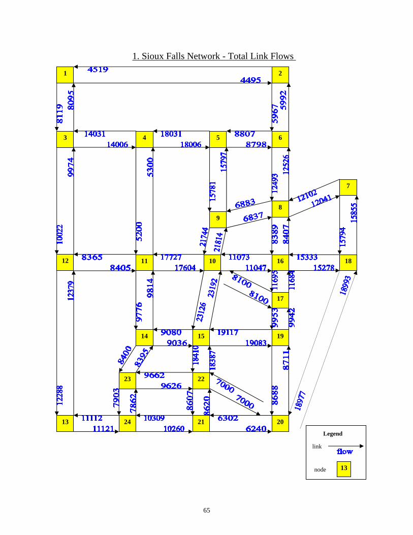
65

Total Link Flows -Sioux Falls Network . 1

node

link

Legend

13

16

9

5

2

6

8

1

3 4

10

7

18 11

19

17

15

22

14

21

23

24 13 20

12

66

1 Node - ased solutionb-Origin. 2

16

9

5

2

6

8

1

3 4

10

7

18 11 12

19

17

15

22

14

21

23

24 13 20

2600 (.060)

1600 (.040) 800 (.07)

2500 (.057)

3000 (.097)

3200 (.023)4500 (.043)

6200 (.040)

2500 (.066)

2200 (.147)

485 (.107)

415 (.020)

915 (.055)

800 (.137) 400 (.163)

15 (.032)

489 (.118)

11 (.122) 389 (.042)

300 (.04)

300 (.043)

1400 (.030)

900 (.177)

311 (.037)

300 (.137)

node

used link

Legend

flow (cost)

13

67

12 Node -based Solution -Origin. 3

16

9

5

2

6

8

1

3 4

10

7

18 11 12

19

17

15

22

14

21

23

24 13 20

227 (.060)

4564 (.040)

5436 (.137) 3319 (.122)

517 (.057)

1156 (.097)

3337 (.023)

3937 (.043)

427 (.040) 127 (.066)

1908 (.147)

446 (.107)

38 (.150)

200 (.020)

900 (.055)

983 (.137)600 (.163)

253 (.201) 0 (.032)

1389 (.118)

11 (.122)689 (.042)

400 (.081)

300 (.043)3900 (.030)

2600 (.177)

710 (.037)

717 (.137)

17 (.122)

1981 (.100)

node

used link

Legend

flow (cost)

13

68

12Node – Route Flow Interpretation. 4

16

9

5

2

6

8

1

3 4

10

7

18 11 12

19

17

15

22

14

21

23

24 13 20

227 (1.0)

4564 (1.0)

5436 (1.0) 3319 (0.87)

517 (0.13)

1156 (1.0)

3337 (1.0)3937 (1.0)

427 (1.0) 127 (0.06)

1908 (0.98)

446 (0.56)

38 (0.02)

200 (1.0)

900 (1.0)

983 (0.98)600 (1.0)

253 (0.44) 0

(0.0)

1389 (1.0)

11 (0.02) 689 (0.98)

400 (1.0)

300 (1.0)3900 (1.0)

2600 (1.0)

710 (1.0)

717 (1.0)

17 (0.02)

1981 (0.94)

node

used link

Legend

flow (prop)

13

h[12,3,4,5,6,8,16] = 1.0 1.0 1.0 0.94 0.98 0.56 700 = 361

69

16 to 2 1s Node-Routes . 5

16

9

5

2

6

8

1

3 4

10

7

18 11 12

19

17

15

22

14

21

23

24 13 20

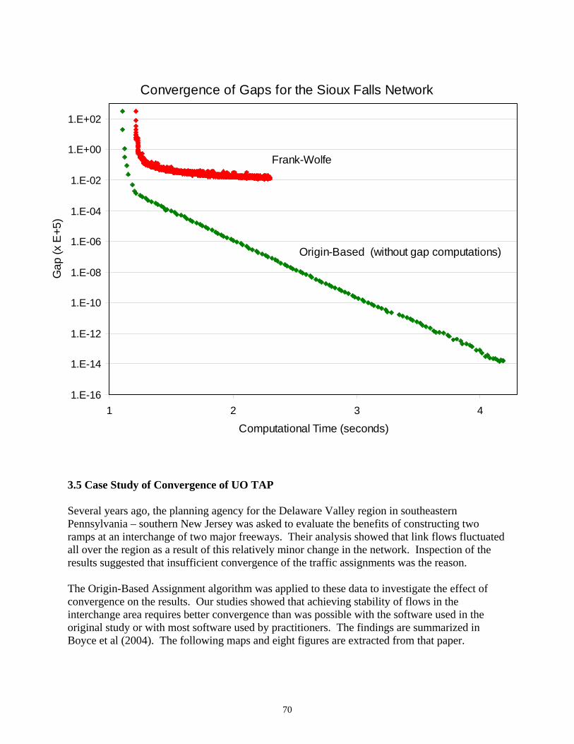
70

3.5 Case Study of Convergence of UO TAP Several years ago, the planning agency for the Delaware Valley region in southeastern Pennsylvania – southern New Jersey was asked to evaluate the benefits of constructing two ramps at an interchange of two major freeways. Their analysis showed that link flows fluctuated all over the region as a result of this relatively minor change in the network. Inspection of the results suggested that insufficient convergence of the traffic assignments was the reason. The Origin-Based Assignment algorithm was applied to these data to investigate the effect of convergence on the results. Our studies showed that achieving stability of flows in the interchange area requires better convergence than was possible with the software used in the original study or with most software used by practitioners. The findings are summarized in Boyce et al (2004). The following maps and eight figures are extracted from that paper.

Convergence of Gaps for the Sioux Falls Network

1.E-16

1.E-14

1.E-12

1.E-10

1.E-08

1.E-06

1.E-04

1.E-02

1.E+00

1.E+02

1 2 3 4

Computational Time (seconds)

Gap

(x E

+5)

Frank-Wolfe

Origin-Based (without gap computations)

71

Fig. 1. Study Area Location in the Delaware Valley Region

In the Figures 3-4, we see that the link flows in the vicinity of the ramps, as well as the ramps themselves, fluctuate substantially as the convergence of the assignment improves from left to right. In Figures 5-6, we can observe the relative error in these link flows, as compared with a highly converged solution. Finally, Figures 7-8 show the fluctuations on a major arterial affected by the introduction of the ramps.

72

Fig. 2. Interchange of I-295 with SR-42 Showing Proposed Ramps Next, we investigated the effect of convergence of the traffic assignments on 8,000 links nearest to the ramps. These results are shown in the next pair of maps. The links are colored in each map according to the difference in link flow between the build and no-build networks, using an order of magnitude scale. For the maps on the next page for Relative Gaps of 1% and 0.0001%, note how the colors change on the west side of the Delaware River, as well as in the vicinity of the ramps, which are shown in the center of the map. A relative gap of 1% may be regarded as best current practice; a relative gap of 0.0001% is well beyond the level of convergence needed for professional practice, but is shown here to illustrate that a precise level of convergence is possible. The next pair of maps shows the errors in the link flow differences, as compared with a very highly converged solution. Note the change in the scale of the color codes in this second pair of maps. For a relative gap of 0.0001%, nearly all link flow differences lie in the interval from +10 to -10.

Delsea Drive

73

Fig. 3. Link flow differences (build less no-build) versus relative gapNew Jersey freeway links with positive flow differences

4,000

6,000

8,000

10,000

12,000

10.0 (6) 1.0 (25) 0.1 (92) 0.01 (534) 0.001 (>2 K) 0.0001Relative Gap in Percent (Equivalent Frank-Wolfe Iterations)

Link

Flo

w D

iffer

ence

s (v

ehic

les

per d

ay)

WB Ramp

EB Ramp

EB I-295 west of Ramps

WB I-295 west of Ramps

NB SR-42 south of Ramps

SB SR-42 south of Ramps

Fig. 4. Link flow differences (build less no-build) versus relative gap New Jersey freeway links with negative flow differences

-8,000

-6,000

-4,000

-2,000

0

10.0 (6) 1.0 (25) 0.1 (92) 0.01 (534) 0.001 (>2 K) 0.0001

Relative Gap in Percent (Equivalent Frank-Wolfe Iterations)

Link

Flo

w D

iffer

ence

s (v

ehic

les

per d

ay)

EB I-295 east of Ramps

WB I-295 east of Ramps

NB SR-42 north of Ramps

SB SR-42 north of Ramps

74

Fig. 5. Error relative to the converged solution versus relative gap New Jersey freeway links with positive flow differences

0.01%

0.10%

1.00%

10.00%

100.00%

10.0 (6) 1.0 (25) 0.1 (92) 0.01 (534) 0.001 (>2 K) 0.0001

Relative Gap in Percent (Equivalent Frank-Wolfe Iterations)

Erro

r Rel

ativ

e to

Con

verg

ed S

olut

ion

WB RampEB RampWB I-295 west of RampsEB I-295 west of RampsNB SR-42 south of RampsSB SR-42 south of Ramps

Fig. 6. Error relative to the converged solution versus relative gap New Jersey freeway links with negative flow differences

0.01%

0.10%

1.00%

10.00%

100.00%

10.0 (6) 1.0 (25) 0.1 (92) 0.01 (534) 0.001 (>2 K) 0.0001

Relative Gap in Percent (Equivalent Frank-Wolfe Iterations)

Erro

r Rel

ativ

e to

Con

verg

ed S

olut

ion

WB I-295 east of RampsEB I-295 east of RampsNB SR-42 north of RampsSB SR-42 north of Ramps

75

Fig. 7. Link flow differences (build less no-build) versus relative gap Delsea Drive crossing I-295 west of SR-42

-400

-200

0

200

400

600

10.0 (6) 1.0 (25) 0.1 (92) 0.01 (534) 0.001 (>2 K) 0.0001Relative Gap in Percent (Equivalent Frank-Wolfe Iterations)

Link

Flo

w D

iffer

ence

(veh

icle

s pe

r day

)

SB Delsea Dr. N of I-295

SB Delsea Dr. at I-295

NB Delsea Dr. N of I-295

NB Delsea Dr. at I-295

Fig. 8. Error relative to the converged solution versus relative gap Delsea Drive crossing I-295 west of SR-42

0.01%

0.10%

1.00%

10.00%

100.00%

1000.00%

10.0 (6) 1.0 (25) 0.1 (92) 0.01 (534) 0.001 (>2000) 0.0001

Relative Gap in Percent (Equivalent Frank-Wolfe Iterations)

Err

or R

elat

ive

to C

onve

rged

Sol

utio

n

SB Delsea Dr. N of I-295NB Delsea Dr. N of I-295SB Delsea Dr. at I-295NB Delsea Dr. at I-295

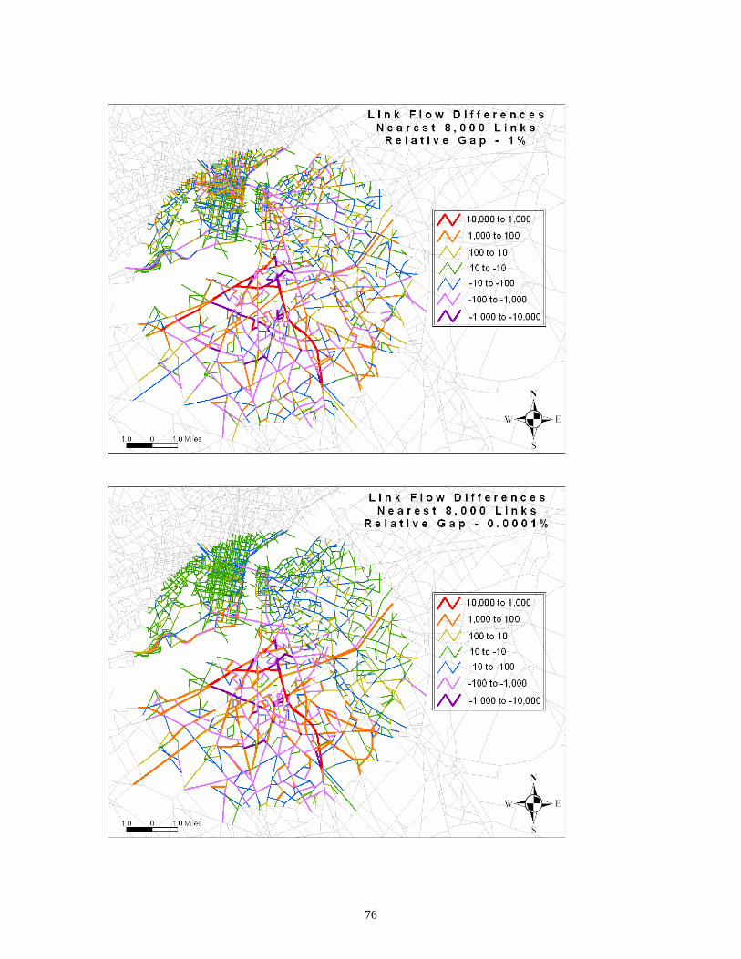
76

77

78

79

80

Error in Link Flow Difference with AEC of 2. min. vs. Link Capacity

-1,000

-500

0

500

1,000

0 10 20 30 40 50 60 70 80 90Link Capacity (1,000s of vehicles per day)

Erro

r in

Link

Flo

w D

iffer

ence

for 2

. min

. AE

C

An Average Excess Cost (AEC) of 2. minutes corresponds roughly to 5-10 iterations of User-Optimal Assignment.

Error in Link Flow Difference with AEC of 0.002 min. vs. Link Capacity

-1,000

-500

0

500

1,000

0 10 20 30 40 50 60 70 80 90Link Capacity (1000s of vehicles per day)

Err

or in

Lin

k Fl

ow D

iffer

ence

for 0

.002

min

. AE

C

An Average Excess Cost (AEC) of 0.002 minutes corresponds to more than 500 iterations of User-Optimal Assignment.

81

TABLE 1. Computational Effort for OBA and Frank-Wolfe Algorithms

Computation effort for the algorithm (h)

Excess costs of origin-based solutions

Relative gap (%)

Equivalent number of

Frank-Wolfe iterations

Frank-Wolfe (EMME/2)

OBA Total (h)

Average (min)

1.0 E + 01 6 0.18 0.96 384,067.9 1.6 E + 00 1.0 E + 00 25 0.64 1.53 28,254.7 1.2 E - 01 1.0 E - 01 92 2.31 2.35 3,129.5 1.3 E - 02 1.0 E - 02 534 13.28 3.41 338.1 1.4 E - 03 1.0 E - 03 >20001 >50.00 5.80 30.1 1.3 E - 04 1.0 E - 04 8.04 3.2 1.4 E - 05 1.0 E - 05 10.82 0.3 1.2 E - 06

1 Relative gap at 2000 iterations = 0.0024% (2.4E-03%) TABLE 2. Delaware Valley Regional Planning Commission Road Network Indicators Indicator congested free-flow1 Average travel time (min) 23.42 17.84 Average travel distance (km) 12.64 12.64 Space-mean-speed (kph) 32.41 42.54 Note: Total flow = 14,336,061 vehicles per day. Total vehicle hours of travel = 4,334,532 h per day. 1 at user-equilibrium flows

Four additional maps show the same results at the regional level. From the first pair, we can observe where changes in link flow differences actually occur as a result of introducing the ramps. From the second pair, showing the errors in link flow differences, we can see that it is possible to achieve a solution that eliminates errors throughout the region covered by these 40,000 links. Finally, two charts show how the errors in link flow differences over the entire region change from the solution with an average excess cost of 2 minutes (relative gap of 10%) to an average excess cost of 0.002 minutes (relative gap of 0.01%). Table 1 provides additional details of the solution by the Origin-based Assignment algorithm and the Frank-Wolfe algorithm widely used in practice, as illustrated here by the EMME/2 software system. 3.6 Dynamic Route Choice on a Road Network This subsection is based on a paper by Boyce, Lee and Ran (2001). For a review of related research, see Peeta and Ziliaskopoulos (2001). This subsection has four objectives. First, we are concerned with predicting route choices of motorists in congested road networks, that is, networks in which travel times depend on

82

congested vehicle flows, which are prevalent in large urban areas. Second, we are interested in dynamic versions of the classic traffic assignment problem, as the problem of predicting motorists’ route choices in a road network is traditionally known. In this context, dynamic means that each variable is time-specific. In fact, dynamic issues enter the problem in several ways:

1. route choices are based on route travel times from origins to destinations that depend on time-dependent link flows;

2. route travel times may refer to the network situation at an instant of time (instantaneous), such as the departure time, or the travel times experienced by travelers during their journeys (actual or ideal);

3. departure flow rates are time-dependent, and ultimately must be regarded as choices that depend on desired arrival times preceded by travel over a dynamically changing road network.

Third, we are interested in analytical representations of these complex phenomena. That is, we seek to formulate a system of equations and inequalities, or equivalent representations, which captures the essence of the physical and behavioral system of interest. The advantages of this approach are several:

1. such representations are specific and precise, although understanding their properties may require extensive analysis;

2. a mathematical formulation can be studied to determine if a solution exists, and whether or not it is unique and stable;

3. solution algorithms to well-formulated models can be devised and their convergence properties determined, both analytically and computationally.

Finally, we are concerned here with model validation; that is, we want to know whether these complex mathematical models predict the observed choices of routes, departure times, link flows, travel times, etc. Efforts to validate models are severely restricted at present by the lack of observations on phenomena of interest. Ironically, such data will likely be provided by the technology that has most motivated research on the dynamic traffic assignment problem: intelligent transportation systems. Dynamic models of travel behavior are needed to plan, design and operate these systems. Through their introduction, we can hope to obtain adequate data, presently unavailable, to validate and further refine the models themselves. In this subsection, we seek to provide an introduction to an approach to this problem, to describe our approach and to discuss issues related to its successful implementation. The subsection is organized in the following way. First, we provide a short overview to indicate the three approaches to formulating the dynamic traffic assignment problem. Second, formulations of two versions of the problem are presented as an example of analytical formulations. Following a brief discussion of solution algorithms, we offer a brief conclusion. Approaches to investigating the analytical dynamic traffic assignment problem can be grouped into three categories: mathematical programming, optimal control theory, and variational inequality. Mathematical programming has a long history in studying the traffic assignment

83

problem stemming from the first formulation of the static traffic assignment problem by Beckmann, McGuire and Winsten (1956); see Patriksson (1994) for the history of the static model. Many algorithms have been proposed and applied to solve mathematical programming-based dynamic traffic assignment models. However, in the context of traffic assignment, mathematical programming has an inherent technical limitation, which sometimes causes it to fail to provide a suitable description of traffic interactions and dynamics, namely the asymmetric nature of travel cost functions and time-dependent interaction of traffic flow and travel time. Optimization formulations generally include integrals of these link cost functions; if the function is asymmetric, its integral is path-dependent, and hence the formulation fails. Optimal control theory by its nature is well suited for describing dynamic systems; hence, its application to modeling dynamic transportation networks is attractive. Several optimal control theory-based models use inflow as the control variable, whereas exit flow is considered to be a function of link flow. Although this formulation provides an explicit relationship between exit flow and link flow, it has several drawbacks:

1. if the exit flow function is concave, it is not possible to establish an optimal control model of the dynamic user-optimal traffic assignment problem with multiple origin-destination pairs;

2. exit flow functions may cause instantaneous flow propagation. The exit flow rate must be positive in order to satisfy the exit flow function; if the initial flow is zero, it causes unrealistic flow propagation;

3. no equivalent optimal control-based model exists if strict link capacities are considered. Despite our contributions to this approach (Ran and Shimazaki, 1989a,b; Ran et al., 1993; Ran and Boyce, 1994), we choose not to emphasize it in this review because its limitations have been demonstrated. Compared with mathematical programming and optimal control, variational inequality (VI) formulations provide a more attractive approach to formulating dynamic route choice problems. VI problems may be regarded as a generalization of constrained optimization problems, complementarity problems, and fixed point problems. Because of its more general properties and capabilities, VI has gained increasing attention during the last decade; see Nagurney (1999) for a review. In the context of dynamic network modeling, issues of asymmetric cost functions and capacitated assignment problems can be accommodated by the VI approach, assuming that certain monotonicity and convexity conditions are met.

3.5.1 Problem Formulation as a Variational Inequality This section summarizes a dynamic route choice model, which can be extended to incorporate motorists’ departure/arrival time choice jointly with route choice (Ran and Boyce, 1996); see also Chen (1999) for a related approach. In the next subsection, some basic definitions and dynamic network flow constraints are stated; Table 1 provides a list of definitions and symbols for convenient reference. Based on actual link travel times, the ideal dynamic user-optimal (DUO) route choice model is then formulated. These formulations are presented to illustrate the concepts and formulation of the dynamic traffic assignment problem using VI methods.

84

Table 1 Definitions and Notation

( )txa number of vehicles on link a at time t ( )txrs

ap number of vehicles on link a and route p between O-D pair rs at time t

( )tua inflow rate of link a at time t ( )tva exit flow rate of link a at time t ( )tvrs

ap exit flow rate of link a on route p between O-D pair rs at time t

( )tE rsp cumulative number of vehicles arriving at destination s from origin r on route p by time t

( )tersp arrival flow rate at destination s from origin r on route p at time t

( )tf rs departure flow rate from origin r toward destination s at time t ( )jA set of links whose tail node is j ( )jB set of links whose head node is j ( )taτ actual travel time over link a for flows entering link a at time t ( )taτ estimated actual travel time over link a for flows entering link a at time t ( )trs

pη travel time actually experienced over route p by motorists departing origin r toward destination s at time t

( )trsπ minimal travel time actually experienced by motorists departing origin r for destination s at time t

( )trsπ estimated minimal travel time actually experienced by motorists departing origin r for destination s at time t

( )trsaΩ perceived actual travel time for flows departing origin r toward destination s over route p

at time t ( )trj

a

∗

Ω difference of the minimal travel time from r to j and the travel time from r to j, via the minimal travel time route from r to i and link a for motorists departing from origin r at time t

raξ departure time interval for flow from zone r on link a

3.5.1.1 Network Flow Constraints The constraint conditions necessary for the formulation of dynamic route choice models are defined first. In addition to flow conservation conditions, flow propagation constraints are emphasized. Other important constraints include link capacity and spillback constraints. The constraint set for a typical VI model is summarized as follows. Relationship between link status and link flow variables:

;,,,)()( srpatvtudt

dx rsap

rsap

rsap ∀−= (1)

85

where )(txrsap is the number of vehicles on link a and route p between OD pair rs at time t,

)(tu rsap is the inflow rate into link a on route p between OD pair rs at time t, and

)(tvrsap is the exit flow rate from link a on route p between OD pair rs at time t.

;,,)()(

rsrptedt

tdE rsp

rsp ≠∀= (2)

where )(tE rsp is the cumulative number of vehicles arriving at destination s from origin r on

route p by time t, and )(ters

p is the arrival flow rate at destination s from origin r on route p at time t.

Flow conservation constraints: ;,)()(

)(srtutf

p

rsap

rAa

rs ∀∑∑=∈

(3)

where )(tf rs is the departure flow rate from origin r toward destination s at time t (given);

;,;,,,)()()()(

srjsrpjtutv rsap

jAajBa

rsap ≠∀∑=∑

∈∈ (4)

;;,)()()(

rssrtetv rs

sBa

rsap

p≠∀=∑ ∑

∈ (5)

where A(j) is the set of links whose tail node is j (after j), and B(j) is the set of links whose head node is j (before j); note that nodes r and s are specific cases of node j. Flow propagation constraints: )()]([)()]([)(

~tEttEtxttxtx rs

parsp

rsbpa

pb

rsbp

rsap −++−+∑=

∈ττ ;,,;);( srprjjBa ≠∈∀ (6)

where p~ denotes the subroute from node j to destination s, and )(taτ is the actual travel time over link a for flows entering link a at time t. Definitional constraints: ;),()(),()( atvtvtutu a

rsp

rsapa

rsp

rsap ∀=∑=∑ (7)

;),()( atxtx arsp

rsap ∀=∑ (8)

86

where )(tua is the inflow rate into link a at time t, )(tva is the exit flow rate from link a at time t, and )(txa is the number of vehicles on link a at time t. Nonnegativity conditions: ;,,,0)(,0)(,0)( srpatvtutx rs

aprsap

rsap ∀≥≥≥ (9)

;,,0)(,0)( srptEte rsp

rsp ∀≥≥ (10)

Boundary conditions: ;,,,0)0( srpErs

p ∀= (11)

;,,,,0)0( srpaxrsap ∀= (12)

3.5.1.2 Model Formulation Dynamic route choice models can be formulated based on either actual or instantaneous travel times. The instantaneous link travel time at time t is defined as the travel time that would be experienced by motorists traversing a link if prevailing traffic conditions remain unchanged. The actual link travel time is the travel time over a link actually experienced by motorists. This time is also called the future or forecast time, since it is not observable at time t. Let )(taτ be the actual travel time over link experienced by motorists entering link a at time t, which is assumed to depend on the number of vehicles ),(txa the inflow )(tua and the exit flow

)(tva on link a at time t. It follows that: atvtutxt aaaaa ∀= )](),(),([)( ττ (13) Similarly, the actual route travel time is the time over a route actually experienced by motorists. Define )(trs

pη as the travel time actually experienced over route p by motorists departing origin r

toward destination s at time t. Using a recursive formula, the route travel time )(trspη can be

computed for all allowable routes. Assume route p consists of nodes ),,,,2,1,( sir LL . Let )(trs

pη denote the travel time actually experienced over route p from origin r to node i by

motorists departing origin r at time t. Then, a recursive formula for route travel time )(trspη is:

).,1(;,,2,1;,,)]([)()( )1()1( iiasiirptttt irpa

irp

rip −==∀++= −− Lητηη

87

The formulation of the ideal DUO route choice problem is based on the underlying choice criterion that each motorist uses the route that minimizes his/her future (actual) travel time when departing from the origin to destination. Thus, for any OD pair under ideal DUO route choice conditions, motorists departing the origin at the same time must arrive at the destination at the same time (Wardrop, 1952). Route-Time-Based Model In this problem, the time-dependent origin-destination trip pattern is assumed to be known a priori. That is, the departure times of motorists are given. The ideal dynamic user-optimal (DUO) route choice problem is to determine the dynamic status of links and the inflow and exit flow variables at each instant of time resulting from motorists using minimal-time routes, given the network, the link travel time functions and the time-dependent OD departure rate requirements. Consider the following dynamic generalization of the conventional static user-optimal state.

Travel-Time-Based Ideal DUO State: If, for each OD pair at each instant of time, the actual travel times experienced by motorists departing at the same time are equal and minimal, the dynamic traffic flow over the network is in a travel-time-based ideal dynamic user-optimal state.

If the actual link travel time )(taτ is determined, the minimal travel time )(trsπ actually experienced by motorists departing origin r for destination s at time t can be computed as

( ))(min)( tt rspp

rs ηπ = . Thus, )(trsπ is a functional of all link flow variables at time w:

]|)(),(),([)( txvut rsrs ≥= ωωωωππ This functional is not available in closed form. Nevertheless, it can be evaluated when

)(),( ωω vu and )(ωx are temporarily fixed. The route-time-based ideal DUO route choice conditions can then be defined as follows: ;,,0)()( srptt rsrs

p ∀≥−∗

πη (14)

;,,0)]()()[( srptttf rsrsp

rsp ∀=−

∗∗∗

πη (15)

.,,0 srpf rsp ∀≥

∗

(16) The asterisk in the above equations denotes that the flow variables are the optimal solutions under the route-time-based ideal DUO state. The equivalent variational inequality formulation of route-time-based ideal DUO route choice conditions (14)-(16) may be stated as follows:

The dynamic traffic flow pattern satisfying network constraint set (1)-(12) is in a route-time-based ideal DUO route choice state if and only if it satisfies the variational inequality problem:

88

∫ ∑ ∑ ≥−∗∗T

rs a

rsp

rsp

rsp dttftft

00)]()()[(η (17)

Solving variational inequality (17) is equivalent to solving ideal DUO route choice conditions (14)-(16). The properties of this formulation are described in Ran and Boyce (1996). Link-Time-Based Model Route-time-based VI models have an intuitive interpretation. With new solution methods, such as disaggregate simplicial decomposition (DSD) or gradient projection (GP), route enumeration is no longer required to obtain a solution to the route-time-based model. However, route-time-based models still require considerable computational effort for networks of realistic size. Therefore, a link-time-based VI model is proposed. The link-time-based ideal DUO route choice conditions given below imply the route-time-based ideal DUO route choice conditions. The set of dynamic network constraints defined above apply to both the link-time-based VI model and the route-time-based VI model. The basic difference between the two models is that the link-time-based model is formulated using link-based flow variables instead of the route-based variables in the route-time-based model. Let )(trj

a

∗

Ω denote the difference of the minimal travel time from r to j and the travel time from r to j via minimal travel time route from r to i and link a for motorists departing from origin at time t: ).,(;,)()]([)()( jiarattttt rjri

arirj

a =∀−++=Ω∗∗∗∗

ππτπ (18) The link-time-based ideal DUO route choice conditions can then be stated as follows: ;),,(0)( rjiatrj

a =∀≥Ω∗

(19)

;,),,(0)(])([ srjiatttu rja

rirsa =∀=Ω+

∗∗∗

π (20)

.,),,(0)]([ srjiattu rirsa =∀≥+

∗

π (21) Link-time-based ideal DUO route choice conditions (19)-(21) imply route-time-based ideal DUO route choice conditions (14)-(16). Then, the equivalent variational inequality formulation of link-time-based ideal DUO route choice conditions (19)-(21) may be stated as follows:

The dynamic traffic flow pattern satisfying constraints (1)-(12) is in a link-time-based ideal DUO route choice state if and only if it satisfies the variational inequality problem:

∫ ∑ ∑ ≥+−+⋅Ω∗∗∗∗T

rs a

rirsa

rirsa

rja dtttuttut

00)]([)]([)( ππ (22)

Solving variational inequality (22) is equivalent to solving link-time-based ideal DUO route choice conditions (19)-(21). Further properties are given in Ran and Boyce (1996). The above models are limited in the sense that the motorists are assumed to be homogenous. One way to

89

relax this assumption is to stratify them into classes, in which each class has distinctly different characteristics. Each class of motorists is associated with a disutility or generalized cost function. Thus, the ideal DUO route choice conditions are defined for each class on the basis of travel disutilities instead of travel time only. Then, a multi-class DUO model can be formulated based on travel costs or disutilities instead of travel times. 3.5.2 Solution Algorithms The link-time-based ideal DUO route choice model is selected as an example for describing a solution algorithm for solving this class of dynamic models. First, the continuous time formulation of the DUO route choice program is transformed into a discrete time VI formulation. Then, the VI model is reformulated as a discrete optimization problem under relaxation and solved using the linearization technique embedded in a relaxation procedure. In the relaxation procedure, the estimated link travel times are updated iteratively and the linearization technique is applied in each iteration to solve the resulting nonlinear programming problem (NLP). For the linearized subproblem, an expanded time-space network can be constructed so that the subproblem can be decomposed according to O-D pairs and can be viewed as a set of minimal-cost route problems. Flow propagation constraints representing the relationship between link flows and travel times are satisfied in the minimal-cost route search so that only flow conservation constraints for links and nodes remain. To convert our continuous VI model into a discrete VI model, the time period [0,T] is subdivided into N small time increments. Each time increment is a unit of time. To simplify the formulation, we modify the estimated actual travel time on each link in the following way so that each estimated travel time is equal to a multiple of the time increment. ,5.0)(5.0if)( +<≤−= iniin aa ττ where i is an integer and Ki ≤≤0 . The continuous VI problem is then reformulated as a discrete VI problem:

∑ ∑ ∑ ≥+−+⋅Ω=

∗∗∗∗N

n rs a

rirsa

rirsa

rja nnunnun

10)]([)]([)( ππ (23)

For each relaxation iteration, we temporarily fix: a) the actual travel time )(naτ in the link flow

propagation constraints as )(naτ ; b) the minimal travel times )(nri∗π as )(nri∗π and )(nrj∗π as

)(nrj∗π for each link and each origin node. Then, the objective function of an optimization problem can be formulated, which is equivalent to the discrete VI under relaxation, as follows:

( ) ( )[ ]( )

( ) ( ) ( )[ ]⎭⎬⎫−∑+∑ ∑

⎩⎨⎧∫= r

arjr

ari

r

ra

k a

ku

aaaExvukudwkvkxZ

a

ξπξπωτ0,,,

,,min (24)

90

where the new time interval index k is defined as )( ra

rirak ξπξ += with departure time interval

raξ calculated by using the above equation once interval k, origin r and arrival node i are given.

Note that both minimal travel times )( ra

ri ξπ and )( ra

rj ξπ are fixed temporarily at each relaxation iteration. In summary, in each relaxation step, we need to solve a discrete NLP consisting of objective function (24) and its associated constraints. To develop an operational dynamic traffic assignment model for real-time applications, computational requirements pose a major challenge. Clearly, more efficient algorithms than the one outlined above are needed. To this end, the continuous variational inequality (VI) is first transformed into a discrete variational inequality. Then, a relaxation method is used to solve this discrete VI. During each relaxation, a nonlinear programming (NLP) problem is formulated and solved. Unlike the previous algorithm, which uses inflow, exit flow and number of vehicles as the basic variables, this new algorithm uses the inflow variable as the only independent variable to formulate the NLP. To solve this NLP using the Frank-Wolfe algorithm, a linear programming (LP) subproblem is formulated in each iteration. One of the major contributions of this new algorithm (Ran et al, 2002) is that it solves the LP subproblem on a representation of the physical network rather than on an expanded time-space network. Thus, the new algorithm avoids the time-space network expansion and searches for shortest routes on the expanded network, the previous method for solving the analytical DTA model. Consequently, the computation time can be shortened substantially. Computational experience on the Sioux Falls network benchmarks the efficiency of this algorithm. 3.5.3 Conclusions and Comments on Recent Developments In this review, we have tried to convey the basic concepts and exciting challenges that characterize analytical dynamic traffic assignment research at present. Except for the pioneering efforts of Merchant and Nemhauser, Friesz and Carey, no one had really thought about dynamics in travel choice modeling as recently as 15 to 20 years ago. Likewise, intelligent transportation systems were unknown. Then everything changed, largely as a result of technological developments in computing and communications. Suddenly, ITS was possible, if not fully operational. As a result, dynamic travel choice models were suddenly in vogue and actually needed. Fortunately, scientific interest and understanding of the necessary mathematical constructs, optimal control theory and variational inequalities, were at hand although not widely understood. The result has been an exciting period of innovation and synthesis, which promises to continue. Since the paper by Boyce, Lee and Ran was published in 2001, research has continued on analytical formulations of dynamic route choice models, as well as simulation-based approaches. It is more apparent today than in 2001 that simulation methods in combination with analytical models are likely to be successful in solving large-scale problems. Simulation methods can be used in place of link travel time functions (eqn. 13) and also to estimate flow propagation (eqn. 6). The use of these methods allows researchers to focus their efforts on model formulation and

91

solution methods, and to be less concerned with devising analytical functions for traffic flow relationships. Even so, care must be exercised to assure that the model properties are respected. 3.6 Transit Route Choice The traditional approach to transit assignment is rather simple: 1. represent all transit submodes (bus, rapid transit, commuter rail, express bus) in on network; 2. find the minimal travel time route from origin zone p to destination zone q considering

access, waiting, boarding, in-vehicle, and transfer times; 3. assign all transit trips from zone p to zone q to the minimal time route (all-or-nothing). Even if all-or-nothing assignment to minimal time routes is regarded as adequate, the problem of representing transit networks is more complex than for auto route choice. Moreover, the use of only one route between each O-D pair is simplistic if the transit network is complex with several options for each trip. While only large cities in North America have such systems, in Europe and Asia, complex systems are more common. The transit assignment method developed by Speiss and Florian (1989) respond to this need for a more complex approach. If competing transit services are offered, the results may be simplistic if it is not used. The desired solution is an allocation of O-D flows over several transit routes which minimizes the total expected (mean) generalized cost including walking, access, waiting, boarding, in-vehicle, transfer and egress times plus fare. References Ahuja, R. K., J. B. Orlin, S. Pallottino and M. G. Scutellà; (2003) Dynamic Shortest Paths Minimizing Travel Times and Costs, Networks 41, 197-205 Bar-Gera, H. (1999) Origin-Based Algorithms for Transportation Network Modeling, Technical Report #103, National Institute of Statistical Sciences, Research Triangle Park, NC. (Ph.D. thesis in civil engineering, University of Illinois at Chicago, 1999); downloadable file available at: http://www.niss.org/downloadabletechreports.html Bar-Gera, H. (2002) Origin-Based Algorithm for the Traffic Assignment Problem, Transportation Science 36, 398-417. Beckmann, M., C. B. McGuire, and C. B. Winsten (1956) Studies in the Economics of Transportation, Yale University Press, New Haven. Bothner, P. and W. Lutter (1982) Ein direktes Verfahren zur Verkehrsumlegung nach dem 1. Prinzip von Wardrop, Arbeitsbericht Nr. 1, Forschungsbereich: Verkehrssysteme, Universität Bremen, Germany. Boyce, D., D.-H. Lee and B. N. Janson (1998) A Variational Inequality Model of an Ideal Dynamic User-Optimal Route Choice Problem, In Transportation Networks: Recent Methodological Advances, Bell, M.G.H., ed., Pergamon, Amsterdam, 289-302. Boyce, D., B. Ralevic-Dekic and H. Bar-Gera (2004) Convergence of Traffic Assignments: How Much Is Enough? ASCE Journal of Transportation Engineering 130, 49-55.

92

Boyce, D., D.-H. Lee and B. Ran (2001) Analytical Models of the Dynamic Traffic Assignment Problem, Networks and Spatial Economics 1, 377-390. Chen, A. and D.-H. Lee (1999) Path-based Algorithms for Large Scale Traffic Equilibrium Problem: A Comparison Between DSD and GP, presented at the 78th Annual Meeting of the Transportation Research Board, Washington, DC. Chen, H.-K. (1999) Dynamic Travel Choice Models. Springer-Verlag, Berlin. Chen, H.-K, C.-W Chang and M.-S. Chang (1999) Comparison of Link-Based Versus Route- Based Algorithms in the Dynamic User-Optimal Route Choice Problem, Transportation Research Record 1678, 242-250. Frank, M. and P. Wolfe (1956) An Algorithm for Quadratic Programming, Naval Research Logistics Quarterly 3, 95-110. Gallo, G. and S. Pallottino (1988) Shortest Path Algorithms, Annals of Operations Research 13, 3-79. Kupsizewska, D. and D. Van Vliet (1999) 101 Uses for Path-based Assignment, Transport Planning Methods: Proceedings of Seminar C held at PTRC Planning and Transport Summer Annual Meeting, University of Sussex, UK. Larsson, T. and M. Patriksson (1992) Simplicial Decomposition with Disaggregated Representation for the Traffic Assignment Problem. Transportation Science 26, 4-17. LeBlanc, L. J. (1975) An Algorithm for the Discrete Network Design Problem, Transportation Science 9, 183-199 Lee, D.-H. (1996) Formulation and Solution of a Dynamic User-Optimal Route Choice Model on a Large-Scale Traffic Network, Ph.D. thesis in civil engineering, Univ. of Illinois, Chicago. Lee, D.-H., A. Chen, and Y. Nie (2000) Computer Experiments and Statistical Analysis on Algorithms for Traffic Assignment Problems, Working Paper, Department of Civil Engineering, National University of Singapore, Singapore. Nagurney, A. (1999) Network Economics, Kluwer Academic Publishers, Boston. Patriksson, M. (1994) The Traffic Assignment Problem, VSP, Utrecht, The Netherlands. Pallottino, S. and M. G. Scutellà (1998) Shortest Path Algorithms in Transportation Models: Classical and Innovative Aspects, Equilibrium and Advanced Transportation Modelling, P. Marcotte and S. Nguyen, eds., Kluwer, 245-281. Peeta, S. and A. K. Ziliaskopoulos (2001) Foundations of Dynamic Traffic Assignment : The Past, the Present and the Future, Networks and Spatial Economics 1, 233-265. Ran, B. and D. Boyce (1994) Dynamic Urban Transportation Network Models, Springer, Berlin. Ran, B. and D. Boyce (1996) Modeling Dynamic Transportation Networks, Springer, Berlin. Ran B., D.-H. Lee and S. Shin (2002) New Algorithm for a Multiclass Dynamic Traffic Assignment Model, ASCE Journal of Transportation Engineering 128, 323-335. Ran, B. and Shimazaki, T. (1989a) A General Model and Algorithm for the Dynamic Traffic Assignment Problem, Proceedings of Fifth World Conference on Transport Research, Yokohama, Japan, 463-477. Ran, B. and Shimazaki, T. (1989b) Dynamic User Equilibrium Traffic Assignment for Congested Transportation Networks, presented at the Fifth World Conference on Transport Research, Yokohama, Japan. Spiess, H. and M. Florian (1989) Optimal Strategies: A New Assignment Model of Transit Networks, Transportation Research 21B, 395-412. Wardrop, J. G. (1952) Some Theoretical Aspects of Road Traffic Research, Proceedings of the Institution of Civil Engineers, Part II 1, 325-378.

93

4. Mode Choice If we view travel choices as a hierarchy, then route choice seems naturally to fall at the lowest level, since it is specific to a travel mode. It is less clear what choice should be considered next in the hierarchy. Since mode choices can be made on a daily basis, assuming a car is available, choice of mode may be regarded as the next choice in this hierarchy, as is assumed here. We will also use the mode choice model to introduce the concept of dispersion of choices. Dispersion refers to a departure from a strict, or deterministic, cost minimizing assumption. We say choices are dispersed to a higher cost alternative, if the choices are not strictly cost minimizing as we assumed was the case with auto route choice case. Actually, we could have introduced this concept in the route choice model, leading to the stochastic route choice model. Since that model has some inherent limitations, we are introducing the dispersion concept here. 4.1 Deterministic Mode Choice First, let’s extend the auto route choice model to include choice of mode. Recall our auto route choice formulation,

( )( ) ( )

∑ ∑

∑

∑ ∫

∈≡

∈∈∈≥

∈∈=

=

∈

∈

pq Rr

arra

pqr

pqRr

r

a

f

a

Aahf

QqPpRrh

QqPpdhst

dxxcz

pq

pq

a

, where

;,0

;,:

min

,

0

δ

hh

Up to now, all flows have been defined as vehicles per hour. Now add a subscript m to denote mode, with a representing the auto mode and t representing the transit mode. Even though we have used the subscript a to denote links, the use of a to represent the auto mode should be clear by its context. The addition of the subscript a to the OD pair pq denotes person flows per hour from zone p to zone q by auto, and likewise t for transit denotes person flows per hour. To be more definite, consider the following relaxation of the auto route choice formulation:

( )( ) ( )

∑ ∈∑≡

∈∈∈≥

∈∈∈≥

∈∈=∑

∈∈=∑

∑ ⋅+∑ ∫⋅=

∈

∈

pq Rr

arra

pqm

pqar

pqm

pqm

pqaRr

r

pqpqtpqt

a

f

a

Aahf

QqPpMmd

QqPpRrh

QqPpdd

QqPpdhst

dcdxxcz

pqa

pqa

a

, where

;,,0

;,0

;,

;,/:

,min

,

0,

δ

η

ηdhdh

94

Note the following additions and changes in the model: 1. A parameter η is added to the objective function term representing auto costs; it represents

the ratio of auto occupants to autos (persons per vehicle), and is called auto occupancy; 2. A second term is added to the objective function denoting total transit costs, where cpqt is the

fixed generalized cost of travel per person by transit from zone p to zone q, and dpqt is the flow of persons from zone p to zone q by the transit mode t;

3. The right-hand-side of the first constraint has been divided by η to convert auto person flows

pqad from zone p to zone q to auto vehicle flows on route r, rh ; 4. A constraint is added requiring that the variable OD flows by mode sum to the fixed total OD

flow; 5. The set of routes by auto has been redesignated as Rpqa. What this formulation states is find the allocation of fixed OD flows to the two modes, and within the auto mode to routes, so as to minimize a function of total generalized cost. Because we want the auto route flows to be User-Optimal, we do not minimize the total cost of auto travel, as we do for transit, but rather retain the sum of the integrals of the links cost functions. Let’s examine the KKT optimality conditions to see how this problem formulation works. The Lagrangean function is defined as follows:

( ) ( ) ( )∑ −+−∑ ⎟⎟⎠

⎞⎜⎜⎝

⎛∑ −−∑ ⋅+∑ ∫⋅=∈ pq

pqpqtpqapqpq Rr

pqarpqapq

pqtpqta

f

a ddddhudcdxxc,Lpqa

a

ρηηρ /,,0

udh

The KKT optimality conditions obtained by taking derivatives of this function with respect to

pqtpqar ddh and , are:

( )

( )

QqPpu

d

QqPpu

QqPpRrufch

QqPpRrufc

pqpqa

pqa

pqpqa

pqapqaa

araar

pqapqaa

araa

∈∈=⎟⎟⎠

⎞⎜⎜⎝

⎛−

∈∈≥−

∈∈∈=⎟⎠⎞⎜

⎝⎛ −∑ ⋅⋅

∈∈∈≥−∑ ⋅⋅

,,0

,,0

,,,0

,,,0

ρη

ρη

δη

δη

( ) QqPpcd

QqPpc

pqpqtpqt

pqpqt

∈∈=−

∈∈≥−

,,0

,,0

ρ

ρ

95

QqPpdd

QqPpd

h

pqm

pqm

Rr

pqar

pqa

∈∈=−∑

∈∈=∑ −∈

;,0

,,0η

0d0h ≥≥ , Clearly, this is rather messy. Let’s see what we can do to clarify matters. First, consider the case of ,0>rh for some OD pair pq. Then, the travel cost, ,/ηpqapqar uc = which is also true for all used auto routes from zone p to zone q. Next, consider the condition related to dpqa. Since we assumed that ,0>rh therefore ,0>pqad and pqpqau ρη =/ , the equilibrium OD cost from zone p to zone q. If ,pqtpq c=ρ then, ;0≥pqtd otherwise, ,pqpqtc ρ> and .0=pqtd Without belaboring the analysis further, we draw the following conclusions about this formulation: 1. If OD flows occur by auto, then all used routes have equal cost, and no unused route has a

lower cost; 2. The costs of the used auto routes not only determine the OD cost, but also determine whether

transit has a sufficiently low cost to be used. If it does, then the OD cost by transit and auto are equal; that is, either there are no transit flows or the transit cost sets a maximum level for the auto costs for each OD pair.

3. If the transit costs are lower than can be achieved by auto, then all OD flows will move by

transit. Hence, the solution is in some sense all-or-nothing with respect to mode. 4. If the auto occupancy η were not included in the objective function, then the auto OD cost would be different from the OD equilibrium cost by a factor equal to η. For consistency of the formulation, then, we see that the weight η is necessary in the objective function. From this analysis, we can see that the formulation of the mode and auto route choice model as a deterministic cost minimization problem may be rather unrealistic, for example, we observe in Census data that both auto and transit flows occur between many, many OD pairs. Therefore, we explore an approach to relax the deterministic nature of the formulation through the addition of a certain constraint known as a dispersion or entropy function.

4.2 Dispersion Constraint What we need to do is to define a constraint that will soften or blur the hard deterministic (all-or-nothing) character of the above model. Not surprisingly, there is a function available for this job, and it has a one-to-one correspondence with a well-known choice function, the logit function. The objective of this subsection is to introduce this function and its properties. Suppose a probability is defined for each discrete value of a variable: xi = the discrete value observed for category i, i = 1, 2, …, N; pi = the probability that xi occurs, or the observed relative frequency with which xi occurs.

96

An example is shown by the following bar chart.

Discrete Probability Bar Chart As we can see in the chart, there are three observed events:

event 2 occurs with observed relative frequency 0.4; event 6 occurs with observed relative frequency 0.1; event 7 occurs with observed relative frequency 0.5.

We would like to characterize these observed frequencies with a single measure indicating how dispersed or clustered they are. One possible response to this question is to compute the mean value of the observed response, and then to compute the variance. However, in this case, we would like a measure that doesn’t depend on the values of the responses, because they are qualitative or nominal values such as mode or OD pair. The measure we propose is defined as:

∑−≡i

ii ppS ln , where S is the measure of dispersion and pi is the observed relative frequency

of event i. This function is known as the entropy function in statistics and information theory. For the case in question, the value of S is 0.9433483, if we agree that .0.00ln0 =⋅ How should we interpret this value? Suppose we agree that the maximum dispersion that can be achieved in the observed events is for them all to have equal frequencies. If there are N possible events, and they have equal relative frequencies, then their relative frequency is 1/N. Let’s compute the dispersion of this case:

( ) ( )( ) ( )( ) ( )NNNNN

NS lnln0ln1ln11ln1max =−−=−⋅−=⎟

⎠⎞

⎜⎝⎛⋅−=

Therefore, the maximum dispersion is the natural logarithm of the number of categories. Note it is a positive number because we were careful to define S with a negative sign. Next, let’s consider the minimum value that S can achieve when the events are completely clustered. That occurs if one event has relative frequency of 1.0; all other events have relative frequencies of 0.0.

1 2 N

ip

ix 0.0

1.0

0.5

6 7

97

( ) ( ) ( )( ) ( ) 0.00.00.00.0ln0.010.1ln0.1min =−=−−⋅−= NS Hence the range of S is 0.0 to ( ).ln N The function S can also be expressed in terms of the observed frequencies, rather than relative frequencies. The two versions are related as follows, where .∑=

iiTT

[ ]∑ ∑∑∑ +−=−−=⎟⎠⎞

⎜⎝⎛

⎟⎠⎞

⎜⎝⎛−=−=

i iiiii

i

ii

iii TTT

TTTT

TTT

TTppS lnln1lnln1lnln

Therefore, ∑ −⋅=−

iii TTSTTT lnln . The sign of the left-hand side is negative, if all of the

observed frequencies are greater than or equal to 1. A constraint can be formed with the dispersion function in the following way. Generally, the cost minimizing solution is the least dispersed feasible solution, since the mode choices strictly take the least cost mode. By constraining the dispersion of choices to be higher than the minimum, some choices are shifted to the higher cost mode. The form of the constraint is

( ) 0ln Sddpqm

pqmpqm ≥− ∑ , where 0S represents the dispersion of the observed modal choices. The

form of this function is concave, as can be seen by plotting S vs. p1, for the case of two probabilities, p1 and p2. Let’s add this constraint to the problem defined in Section 4.1, but first simplify the problem definition to exclude route flows by fixing auto costs, as follows. Fixed Cost Assignment Problem with Deterministic Mode Choice

( )

( )

QqPpMmd

QqPpddst

dcz

pqm

pqm

pqm

pqmpqmpqm

∈∈∈≥

∈∈=∑

∑ ⋅=

;,,0

;,:

min dd

where qpmc pqm zone to zone from modeby travelofcost fixed = qpmd pqm zone to zone from modeby flow travel= Adding the dispersion constraint, we obtain: Fixed Cost Assignment Problem with Stochastic Mode Choice

( )( )

QqPpMmd

Sdd

QqPpddst

dcz

pqm

pqmpqmpqm

pqm

pqm

pqmpqmpqm

∈∈∈≥

≥∑−

∈∈=∑

∑ ⋅=

;,,0

ln

;,:

min

0

dd

98

The Lagrangean is:

( ) ⎟⎠⎞

⎜⎝⎛ −∑−−∑ −+−∑ ⋅=⎟⎟

⎠

⎞⎜⎜⎝

⎛0ln11,, SddddddcL

pqmpqmpqm

pqpqpqtpqapq

pqmpqmpqm µ

ρµ

ρd

Note that in the Lagrangean, the entropy term is multiplied by (-1), so the overall term is convex. The optimality conditions are:

( ) ( )

( ) ( )

0ln1

ln

0

01ln11

01ln11

0

0

=⎟⎟⎠

⎞⎜⎜⎝

⎛−−

≥−

=−+

=−−−+−

=−−−+−

∑

∑

Sdd

Sdd

ddd

dc

dc

pqmpqmpqm

pqmpqmpqm

pqpqtpqa

pqtpqpqt

pqapqpqa

µ

µρ

µρ

Since the person flows are the arguments of logarithmic functions, they all must be positive; otherwise, we would have ( ) −∞⇒0ln . Hence we can delete the complementary slackness constraints on .pqmd Considering the first two conditions, we obtain:

( )( )( ) QqPpMmcd

cd

pqmpqpqm

pqmpqpqm

∈∈∈−−=

−−=

,,,1exp

so ,1ln

ρµ

ρµ

Summing the expressions for auto and transit,

( ) ( )

( ) ( )⎟⎠⎞⎜

⎝⎛∑ ⋅−=−⋅⇒

∑ ⋅−⋅∑ −==

mpqmpqpq

mpqm

mpqpqpqm

cd

cdd

µρµ

µµρ

exp/1exp

exp1exp

Substituting this expression into the equation for dpqm, we obtain:

( )( )

( )( ) ,

expexp

or ,exp

exp|

⎟⎟⎟

⎠

⎞

⎜⎜⎜

⎝

⎛

∑ ⋅−

⋅−=

⎟⎟⎟

⎠

⎞

⎜⎜⎜

⎝

⎛

∑ ⋅−

⋅−=

npqn

pqmpqm

npqn

pqmpqpqm c

cd

cc

ddµµ

µµ

where =≡ pqpqmpqm ddd /| conditional probability of choosing mode m, given OD pair pq. Thus, the optimality conditions for this problem correspond to the multinomial logit model with cost sensitivity parameter µ , the reciprocal of the Lagrange multiplier of the dispersion constraint.

99

4.3 Combined Mode and Route Choice Model Before proceeding to an examination of the properties of the logit model, let’s synthesize the above results. The original formulation with the dispersion constraint inserted is:

( )( ) ( )

( )

∑ ∑

∑

∑

∑

∑∑ ∫

∈≡

∈∈∈>

∈∈∈≥

≥−

∈∈=

∈∈=

⋅+⋅=

∈

∈

pq Rr

arra

pqm

pqar

pqmpqmpqm

pqm

pqm

pqaRr

r

pqpqtpqt

a

f

a

Aahf

QqPpMmd

QqPpRrh

Sdd

QqPpdd

QqPpdhst

dcdxxcz

pqa

pqa

a

, where

;,,0

;,0

ln

;,

;,/:

,min

,

0

0,

δ

η

ηdhdh

The revised Lagrangean is defined as follows.

( ) ( )

( ) ( ) ⎟⎟⎠

⎞⎜⎜⎝

⎛−−−−+−

⎟⎟⎠

⎞⎜⎜⎝

⎛−−⋅+⋅=

∑∑

∑ ∑∑∑ ∫∈

0

0

ln1

/,,

Sddddd

dhudcdxxcρ,L

pqmpqmpqm

pqpqpqtpqapq

pq Rrpqarpqa

pqpqtpqt

a

f

apqa

a

µρ

ηηudh

The optimality conditions derived by taking derivatives of this function are stated below.

( )

( )

( )( )

( )( ) QqPpdc

QqPpdu

QqPpRrufch

QqPpRrufc

pqtpqpqt

pqapqpqa

pqapqaa

araar

pqapqaa

araa

∈∈=++−

∈∈=++−⎟⎟⎠

⎞⎜⎜⎝

⎛

∈∈∈=⎟⎠⎞⎜

⎝⎛ −∑ ⋅⋅

∈∈∈≥−∑ ⋅⋅

,,01ln1

,,01ln1

,,,0

,,,0

µρ

µρ

η

δη

δη

QqPpdd

QqPpd

h

mpqpqm

Rr

pqar

pqa

∈∈∑ =

∈∈=∑ −∈

;,

,,0η

100

( )

( )0d0h ≥≥

=⎟⎠⎞

⎜⎝⎛ −∑−

≥∑−

,

0ln1

ln

0

0

Sdd

Sdd

pqmpqmpqm

pqmpqmpqm

µ

For routes with positive flow, ,,0 pqar Rrh ∈> the UO travel cost is:

( ) pqaa

araa

pqa cfcu

≡⋅= ∑ δη

; therefore,

( )

( ) 01ln1

01ln1

=++−

=++−

pqtpqpqt

pqapqpqa

dc

dc

µρ

µρ

which are the same conditions found above for the case of fixed auto costs. Therefore, for the combined mode and route choice model, the mode choice function is given by:

( )( )⎟⎟

⎟

⎠

⎞

⎜⎜⎜

⎝

⎛

∑ ⋅−

⋅−=

npqn

pqmpqpqm c

cdd

µµ

expexp

and the usual UO conditions hold for auto route costs. This completes the derivation of a model that combines mode and route choice models, which is therefore known as a combined model. 4.4 Properties of the Logit Model Consider a model of choice of two modes, auto a and transit t:

( )

( ) ( ) ( )( )pqapqtpqtpqa

pqapqa

pq

pqa

ccccc

Pdd

−⋅−+=

⋅−+⋅−⋅−

=≡µµµ

µexp1

1expexp

exp|

Thus, probability of using mode a, ,| pqaP depends on ( )pqapqtpq ccc −=∆ . From the following figure, we can see the role of the dispersion parameter µ is to determine to what extent travelers prefer the lower cost mode. If ,2.0=µ then the choice shifts from transit to auto within a small range of the cost difference .pqc∆ If ,0=µ there is no preference between modes. An important property and shortcoming of the Logit model concerns how the model responds to the addition of a new choice alternative. This property is known as the “independence of irrelevant alternatives” or IIA, property. Because the model is extremely simple, it treats each alternative mode independently without considering whether its attributes are similar to another

101

An Example of a Logit Function Applied to Mode Choice

mode; i.e. it ignores the correlation of modal attributes. Consider the ratio of two choice probabilities:

( )( )pqt

pqa

pqt

pqa

cc

kPP

⋅−

⋅−==

µµ

expexp

|

|

Now suppose a new mode t' is added. Since the denominator term ( )∑ ⋅−

npqncµexp doesn't

affect ,/ || kPP pqtpqa = then the ratio of the mode choices remains constant when the new mode is added. For example,

1. Before the new mode is added: kPP

PP

ta

ta

==+

/1

, so, .1

,1

1+

=+

=k

kPk

P at

2. After the new mode t' is added: kPPPPP

ta

tta

==++ ′

/1

05.0=µ

2.0=µ

1.0=µ

0.0=µ

pqapqtpq ccc −=∆

pqaP |

102

Assume that mode t' has the same characteristics as mode t, so ,1/ =′tt PP ( ) 2/1 +== ′ kPP tt and ( ).2/ += kkPa Even though mode t' has the same characteristics as mode t, mode a loses a portion of its market to t', rather than the market of mode t being divided in half. For example, if

k = 3, then 41 and

43

== ta PP before mode t' is introduced. Afterwards, .51;

53

=== ′tta PPP

Thus the market for t and t' is 40% compared to 25% for mode t alone. (We assume the service attributes of t and t' together did not change.) This property is often referred to as the “red bus/blue bus” problem since the color of a new mode should not affect mode choice. 4.5 Nested Logit Model and Composite Costs One method for addressing the IIA property is to define a nested logit model. Consider two modes, a and t, and two submodes of mode t, r and s, as shown in the following figure.

Decision Tree for Two Modes and Two Submodes Then,

( )( )∑

∈

⋅−⋅−

=

tRss

rtr c

cPθ

θexp

exp|

where trP | = conditional probability of using submode r θ = dispersion parameter related to submode choice Rt = set of all submodes of mode t

The composite cost of transit tc~ can then be defined by setting: ( ) ( )∑

∈⋅−≡⋅−

tRsst cc θθ exp~exp

Taking natural logs, we obtain ( )⎟⎟⎠

⎞⎜⎜⎝

⎛⋅−−= ∑

∈ tRsst cc θ

θexpln1~

tc~ is the expected (mean) cost experienced by an individual traveler drawn at random from the

group using transit. Then, the nested mode choice model for submode r is:

auto - a transit - t

rail - r bus - s

103

( )( )

( )( )⎟⎟

⎟

⎠

⎞

⎜⎜⎜

⎝

⎛

∑ ⋅−

⋅−⋅⎟⎟⎟

⎠

⎞

⎜⎜⎜

⎝

⎛

∑ ⋅−

⋅−=

∈ tRspqs

pqr

npqn

pqtpqtr c

cc

cP

θθ

µµ

expexp

exp

~exp

An alternative to using the nested formulation is a generalization of the dispersion (entropy) function, as follows:

∑ ⎟⎟⎠

⎞⎜⎜⎝

⎛−=

pqm pqm

pqmpqm Q

ddS ln

where =pqmQ prior probability of travel from zone p to zone q by mode m. The effect of adding the prior probability term may be determined as follows:

( )( )⎟⎟

⎟

⎠

⎞

⎜⎜⎜

⎝

⎛

∑ ⋅−⋅

⋅−⋅=

npqnpqn

pqmpqmpqpqm cQ

cQdd

µµ

expexp

Now, reconsider the addition of a new transit mode. Initially, ,5.0== pqtpqa QQ with the result that the prior probabilities cancel out. But suppose that .25.0;5.0 === pqspqrpqa QQQ Then,

( )

( ) ( ) ( )⎟⎟⎠⎞

⎜⎜⎝

⎛

⋅−⋅+⋅−⋅+⋅−⋅

⋅−⋅=

pqspqrpqa

pqapqpqa ccc

cdd

µµµµ

exp25.0exp25.0exp5.0exp5.0

Now, if ,pqrpqs cc =

( )

( ) ( ) ( )⎟⎟⎠⎞

⎜⎜⎝

⎛

⋅−⋅+⋅−⋅+⋅−⋅

⋅−⋅=

pqrpqrpqa

pqapqpqa ccc

cdd

µµµµ

exp25.0exp25.0exp5.0exp5.0

( )

( ) ( )⎟⎟⎠⎞

⎜⎜⎝

⎛

⋅−⋅+⋅−⋅

⋅−⋅=

pqrpqa

pqapq cc

cd

µµµ

exp5.0exp5.0exp5.0

which is the intuitively expected result. Hence the “red bus-blue bus” problem can also be treated through the use of prior probabilities.

104

Exercises 1. Deterministic Mode Choice The formulation of the combined auto route choice and mode choice problem takes the view that origin-destination flows by mode ( pqad , pqtd ) are defined in persons per hour, but auto route choice flows ( rh ) are defined in vehicles per hour, as shown in the following constraint: QqPpdh pqa

Rrr

pqa

∈∈=∑∈

;,/η

and ∑ ∑ ∈≡∈pq Rr

arra Aahf

pqa

,δ

Clearly, this is one possibility, but another definition is equally plausible: QqPpdh pqa

Rrr

pqa

∈∈=∑∈

;,

and ∑ ∈∑≡∈pq Rr

arra Aahf

pqa

,/ηδ

where auto link flows are in vehicles per hour and auto route flows are in persons per hour. Reformulate and solve the combined user-optimal auto route and mode choice problem stated in Section 4.1 with this second definition. Is the auto occupancy term (η ) still needed in the objective function? 2. Regional Mode Choice Constraint A desirable feature of a mode choice model is that it predicts the overall regional mode share correctly. That is, the ratio of the sum of the transit demand summed over all origin-destination pairs to total regional demand ought to equal an exogenous estimate of that demand derived from base year data. ∑⋅=∑

pqpqt

pqpqt dMd

where tM = exogenous estimate of the regional transit share To determine the implications of this requirement, add the above equation as a constraint to the combined auto route and mode choice problem stated in Section 4.3. What is the effect of the constraint on the modal cost structure? Can you offer an interpretation of the new cost term in the model?

105

3. Mode Choice Parameter Estimation I suggest you do this exercise in Excel; submit your plots in printed form. Suppose a home-to-work trip by commuter railroad from the Chicago suburb of Evanston to the Chicago central area requires 60 generalized cost minutes; that is, the generalized cost in units of minutes, which consists of a weighted combination of travel time and fare, is pqtc = 60. The generalized cost for the same trip by auto is pqac = 40 minutes. Assuming that the mode choice is given by the following function, determine how the proportion of trips by auto (a) varies with the cost sensitivity parameter µ . That is, plot pqaP | vs. µ for values ranging from 0.0001 to 10, a possible range for µ . Use the log scale for plotting µ .

( )

( ) ( ) ( )( )pqapqtpqtpqa

pqapqa cccc

cP

−⋅−+=

⋅−+⋅−⋅−

=µµµ

µexp1

1expexp

exp|

The Chicago area planning authority wants to introduce road prices that will cause more travelers to choose transit. The possibilities for tolls range from $1.00 to $4.00. Assuming that the travelers’ mean value of time is $12.00 per hour, investigate what effect this range of tolls will have on their mode choice. To present your results, plot pqaP | vs. µ for each toll in increments of one dollar. Explain what happens, according to the logit model, when the toll reaches the level that the generalized cost of travel by car exceeds that of transit.

106

5. Origin-Destination Choice (Trip Distribution) The origin-destination choice (trip distribution) problem is to find the flow (persons/hour) from each origin zone to each destination zone, given the total flows leaving each origin and entering each destination, and the interzonal travel costs, as shown below. Origin-Destination Flows

1 2 . . q . . Q Total

1 d11 d12 … … d1q … … d1Q O1 2 d21 d22 … … d2q … … d2Q O2 . … … … … … . … … … … … p dp1 dp2 … … dpq … … dpQ Op . … … … … … . … … … … … P dP1 dP2 … … dPq … … dPQ OP

Total D1 D2 … … Dq … … DQ d..

Travel Costs

1 2 . . q . . Q 1 c11 c12 … … c1q … … c1Q 2 c21 c22 … … c2q … … c2Q . … … … … . … … … … p cp1 cp2 … … cpq … … cpQ . … … … … . … … … … P cP1 cP2 … … cPq … … cPQ

where dpq = flow from origin zone p to destination zone q (persons/hour) cpq = travel cost from origin zone p to destination zone q Op = flow departing from origin zone p Dq = flow arriving at destination zone q ∑∑=

p qpqdd .. = total flow departing from and arriving at all zones

The general form of the traditional model is ( )pqqqpppq cfDBOAd = where pA is a factor related to origin zone p; qB is a factor related to destination zone q;

( )pqcf is a non-increasing function of pqc such as ( ) ( ) .or exp αβ −⋅− pqpq cc

107

Originally, such models were highly empirical and based on an analogy with the gravity law describing the attractive force between two masses, hence, the commonly used name, gravity model. The name comes from the fact that nearby zone pairs have higher flows than more separated zones. In the mid 1960's, several authors showed that such a functional form could be derived using statistical methods without reference to gravitational concepts from physics. 5.1 Model Derivation Our derivation extends the fixed cost derivation of the mode choice model by relaxing the constraint that pqd is known. The focus of this subsection is on the calculation of pA and qB . First, replace the constraint, QqPpdd

mpqpqm ∈∈=∑ ;, with constraints defined on the origin

and destination flows, Op and Dq. The dispersion constraint is also generalized implicitly to describe dispersion to higher cost destinations as well as modes.

( )( )

QqPpMmd

Sdd

QqDd

PpOdst

dcz

pqm

pq mpqmpqm

p mqpqm

pq m

pqm

pqmpqmpqm

∈∈∈≥

≥−

∈=

∈=

⋅=

∑∑

∑∑

∑∑

∑

;,,0

ln

,

;,:

min

0

dd

For ,0>pqmd that is for positive flows between all origin-destination pairs and for all available modes, the solution is ( )( ) ( )pqmqppqmqppqm ccd ⋅−+−≡−−′+′= µλκλκµ 1exp1exp where

qp λκ ′′ and are Lagrange multipliers associated with the constraints on origin and destination flows, and µ is associated with the dispersion constraint, as in the mode choice model. We can express these parameters in terms of the flows as follows:

( ) ( ) ( ) ( )

( ) ( ) ( ) ( )∑∑ ∑∑ ∑ ⎟⎠⎞⎜

⎝⎛ ∑ ⋅−−=⋅−+−==

∑∑ ∑∑ ∑ ⎟⎠⎞⎜

⎝⎛ ∑ ⋅−−=⋅−+−==

p m p m p mpqmpqpqmqpqpqm

q m q m q mpqmqppqmqpppqm

ccDd

ccOd

µκλµλκ

µλκµλκ

exp1expexp1exp

expexp1exp1exp

Hence,

( )( ) ( )

( )( ) ( )

. exp1exp

exp ;expexp

1exp∑ ⎟

⎠⎞⎜

⎝⎛ ∑ ⋅−−

=∑ ⎟

⎠⎞⎜

⎝⎛ ∑ ⋅−

=−

p mpqmp

qq

q mpqmq

pp

c

D

c

O

µκλ

µλκ

Substituting into the original expression, we obtain:

108

( )

( ) ( ) ( ) ( )∑ ⎟⎠⎞⎜

⎝⎛ ∑ ⋅−⋅−⋅∑ ⎟

⎠⎞⎜

⎝⎛ ∑ ⋅−⋅

⋅−=

p mpqmp

q mpqmq

pqmqppqm

cc

cDOd

µκµλ

µ

exp1expexpexp

exp

Hence, we have not eliminated , and qp λκ but only rearranged them, which must be true because they are functions of each other. But, we can see that we can define two sets of balancing factors:

( ) ( ) ( ) ( )

.,exp1exp

1;,expexp

1 Qqc

BPpc

A

p mpqmp

q

q mpqmq

p ∈∑ ⎟

⎠⎞⎜

⎝⎛ ∑ ⋅−−

=∈∑ ⎟

⎠⎞⎜

⎝⎛ ∑ ⋅−

=µκµλ

By substitution, ( )pqmqqpppqm cDBOAd ⋅−= µexp Thus, the flow from zone p to zone q on mode m is directly proportional to the flow leaving zone p, Op, the flow entering zone q, Dq, and a deterrence function defined on cpqm, as well as balancing factors Ap and Bq. Moreover, Ap and Bq are functions of all destination flows and all origin flows, respectively, since

( ) ( )

.,exp

1;,exp

1 QqcOA

BPpcDB

A

p mpqmpp

q

q mpqmqq

p ∈⎟⎠

⎞⎜⎝

⎛⋅−

=∈⎟⎠

⎞⎜⎝

⎛⋅−

=

∑ ∑∑ ∑ µµ

Moreover, by definition, ( )∑ ⋅−=∑=

mpqmqqpp

mpqmpq cDBOAdd µexp

Define ( )⎟⎠⎞⎜

⎝⎛∑ ⋅−−=

mpqmpq cc µ

µexpln1~ . Then ( )pqqqpppq cDBOAd ~exp ⋅−= µ

More generally, this model may be extended to:

( ) ( )( )∑ ⋅−

⋅−⋅⋅−=

npqn

pqmpqqqpppqm c

ccDBOAd

µµ

βexp

exp~exp

so that the mode choice is determined jointly with the origin-destination choice.

109

5.2 Computation of Ap and Bq The following method is commonly used to compute Ap and Bq. The method is known to converge under very general conditions. Step 0. ( )pqqqppqp cDBOdPpA ~exp then ;,...1 ,1set 111 ⋅−=== β Step 1. :,...1 ,for solve 1 QqBq =

( ) ( )∑∑∑ ⋅−=⇒⋅−==

ppqp

qp

pqpqqp

qpq cOBcODBDd ~exp

1~exp 11

ββ

Step 2. :,...1 ,for solvenext 2 PpAp =

( ) ( )∑∑ ∑ ⋅−=⇒⋅−==

qpqqq

pq q

pqqqppppq cDBAcDBOAOd ~exp

1~exp 1212

ββ

Step 3. :,...1 ,for solvenext 2 QqBq =

( )∑ ⋅−=⇒

ppqpp

q cOAB ~exp

12

2

β

In general,

( ) ( ) QqcOA

BPpcDB

A

ppqp

kp

kq

qpqq

kq

kp ,...1 ,~exp

1;,...1 ,~exp1

1 =⋅−

==⋅−

=∑∑ − ββ

Continue until

( ) ( )

. all ,; all ,11

qB

BBp

AAA

kq

kq

kq

kp

kp

kp εε <

−<

− −−

For 2000 zones and ε = 10-6, the values of the P + Q parameters are obtained in about 100 iterations. If the procedure does not converge, usually it means that the value of β is too large. In addition, for convergence it must be true that ..dDO

qq

pp == ∑∑ , the total flow in the region.

The use of origin and destination constraints is a rigorous and operational method for imposing assumed origin and destination flows on the model, or on any O-D flow matrix.

110

5.3 Calibration of Travel Deterrence Parameters A remaining problem is to determine the appropriate value of the parameter β. While this parameter is related to the dispersion constraint, it is better chosen with respect to the mean cost,

since this value 0c can be estimated from survey data: ∑ ⋅=pq

pqpq cdd

c ~..

1 . By substituting

values of β into the model and solving it, a curve of the shape shown below can be determined. The figure shown above is based on the Sioux Falls trip matrix of LeBlanc et al (1975). The zone-to-zone travel costs used in preparing the figure are from the user-optimal assignment of LeBlanc’s trip matrix to the Sioux Falls network. Using these travel costs, and the row and column sums of his trip matrix, the trip distribution model was solved for values of the parameter β , the mean costs computed, and plotted. The value of the mean travel cost for LeBlanc’s matrix is 20.7, which has a corresponding value of β = 0.029. The value of the travel cost for β = 0.0 is 23.7. This is the travel cost that corresponds to the trip distribution function,

..dDO

d qppq

⋅= . From these results, we can see that interzonal flows in LeBlanc’s matrix are

close to being proportional to the row and column sums, which is not very representative of observed travel.

Mean Travel Cost vs. Deterrence Parameter

β - deterrence parameter 0β

mea

n tra

vel c

ost

c

0c

111

If an observed value of 0c is available from survey or census data, and the zone-to-zone travel costs ( )pqc~ are known, then the value of 0β can be found by trial and error or by an iterative technique. Since the value of β also depends on the scale of c (minutes vs. hours, for example), a reasonable first guess is ./1 01 c=β Once ( )11 βc is determined by solving the trip distribution model for 1β , then an iterative scheme is given by ( ) ./ 0111 cc nnnn −−− ⋅= βββ Iterate until ( ) .0cc nn ≈β Since β depends on the mean observed generalized cost, it is important to know how travel times and distances are changing over time. Analysis of survey and census data for a sequence of years can be helpful in understanding how travel times and costs have changed, or not changed, whichever is the case. 5.4 Form of the Deterrence Function Until now, only the negative exponential form of the deterrence function has been considered. This function follows from the entropy constraint, and is consistent with the logit function. Other functional forms, however, have been considered in the literature. See Erlander and Stewart (1990) for a definitive review and derivation of alternatives. A simple way to derive one alternative deterrence function is to assume that origin-destination flows are determined by the natural logarithm of travel costs, rather than the travel costs directly. The travel behavior literature does offer some basis for such an assumption, as is discussed further below.

( )( ) ( )

QqPpMmd

Sdd

QqDd

PpOdst

dcz

pqm

pq mpqmpqm

p mqpqm

pq m

pqm

pqmpqmpqm

∈∈∈≥

≥−

∈=

∈=

⋅=

∑∑

∑∑

∑∑

∑

;,,0

ln

,

,:

lnmin

0

dd

In this case, the optimality condition becomes

( )( ) ( ) ( ) αλκαλκ −⋅+=−+= pqmqppqmqppqm ccd explnexp

This power function has a somewhat different shape than the negative exponential function, especially for small values of travel cost; of course, the function also approaches infinity as travel cost approaches zero.

112

These two functions may be combined to derive the Tanner (1961) function, which is noted for its flexibility.

( )( ) ( )

QqPpMmd

Sdd

QqDd

PpOdst

dcdcz

pqm

pq mpqmpqm

p mqpqm

pq m

pqm

pqmpqmpqmpqmpqm

∈∈∈≥

≥−

∈=

∈=

⋅⋅+⋅=

∑∑

∑∑

∑∑

∑

;,,0

ln

,

,:

lnmin

0

αdd

In this case, the resulting function is ( )( ) ( ) ( ) ( ) αβλκαβλκ −⋅⋅−⋅+=⋅−⋅−+= pqmpqmqppqmpqmqppqm ccccd expexplnexp The Tanner function is the most general considered here, in that it includes the exponential and power functions as special cases. A drawback of the Tanner function is that there is no known way to derive it in the user-optimal framework. As applied in practice, the values of β and α have opposite signs. Thus, if the values of β and α are positive, the functions are either

( ) ( ) ( ) αβλκ +⋅⋅−⋅+= pqmpqmqppqm ccd expexp or ( ) ( ) ( ) αβλκ −⋅⋅+⋅+= pqmpqmqppqm ccd expexp Finally, Professor Dieter Lohse (2002) has proposed the EVA function: ( ) ( )( )( )pqmc

pqmpqm cd ⋅−+−+= βδγ exp1/1 He suggests this function leads to better fits to German data. The properties of these four functions can be explored by computing their elasticities. The elasticity of a demand function is the proportional change in demand relative to a given proportional change in cost. That is,

cdcd

cc

dd

e ∂∂

=∂

∂

=

Applying this procedure, we obtain the following results.

113

Name Cost function Elasticity

Negative exponential:

( )cd ⋅−= βexp c⋅− β

Power: α−= cd α−

Tanner: ( ) αβ −⋅⋅−= ccd exp c⋅−− βα

EVA ( ) ( )( )( )ccd ⋅−+−+= βδγ exp1/1 ( ) ( ) ( )

( )⎥⎦⎤

⎢⎣

⎡⋅−+⋅−⋅

⋅++⎟⎠⎞

⎜⎝⎛+

⋅⋅−+

⋅−ccc

ccc

βδβδβ

βδγ

exp1exp1ln

11

exp1

At the end of this section, these functions and their elasticities are plotted. 5.5 Extension to Tours The above traditional treatment of origin-destination flows considers that travelers move from one origin to one destination. Actually, travel frequently consists of visits to a sequence of activities, or a tour. In this section results pertaining to representation of such tours are presented as an example of how to apply this approach to create new models. To provide an idea of the frequency of such tours for travel that begins at home in the morning peak period, consider the following table compiled from a household survey for the Tucson, Arizona region in 2003 by Ms. Yuhwa Lee, a transportation engineering graduate student at the University of Arizona.

Origin 1st destination 2nd destination Number Home Work -- 734 Home School -- 655 Home Serve passenger -- 120 Home Recreation -- 72 Home Shopping, etc. -- 82 Home Serve passenger Work 144 Home Eat meal Work 43 Home Shopping Work 34 Home Other Work 26 Home Serve passenger School 49 Home Other School 35 Home Other longer tours 210 Home All destinations 2204

We consider only the case of fixed travel costs; however, the model can be generalized to the case of endogenous travel costs. Also, to simplify the presentation, only one mode is considered. The basic idea of the model is to generalize the concept of a 2-way trip table shown in section 5.1 to an n-way table. Thus travel from home to an intermediate stop, followed by a travel to work or school can be represented as a 3-way table. In keeping with standard trip generation analysis, we assume that the number of trips per time period is forecast at the home origin by tour type. Typical morning tours are:

114

1. Home – work 2. Home – recreation – work 3. Home – serve_passenger – work 4. Home – eat_meal – school 5. Home – shop-personal_business – recreation

The concept of the 2-way vs. 3-way tables may be visualized as follows: We can formulate the three-way problem as follows for home-shop-work (hsw) travel:

( )( ) ( )

wr

wr

q

hswqr

sq

sq

sq

r

hswqr

sq

sq

p

hswpq

hswp

hswp

q

hswpq

qr

hswqr

hswqrsw

pq

hswpq

hswpqhs

qr

hswqrqr

pq

hswpqpq

rDd

qDOd

qDd

pOd

dddddcdc

ρ

η

λ

κ

αα

,

,

,

, :stmultiplier

1ln11ln1min

∀=∑

∀==∑

∀=∑

∀=∑

∑ −+∑ −+∑+∑

∗

∗

∗

∗

∗∗∗∗∗∗d

Note that the first two terms are equivalent to the total travel cost, .∑ ⋅

pqr

hswpqrpqr dc Moreover, hsw

pqd ∗

denotes the hsw flows from zone p to zone q, which pertains to home-shop travel. Similarly, hswqrd∗ pertains to the same flows from zone q to zone r. Thus zone p is associated with the home

activity, zone q with the shop activity and zone r with the work activity. Dispersion terms are included for each activity pair; origin and destination constraints govern all tours departing from residences in zone p, arriving at zone q for shopping, departing from shopping activities in zone q, and arriving at zone r for work. The optimality conditions are as follows:

Two-way Flows: home-work

hom

e

work

Three-way Flows: home-shop-work

hom

e

shop

work

115

( )( ) ( ) ( )( )( ) ( ) ( )qr

swwr

wr

sq

sqqr

swwr

sq

swhswqr

pqhss

qsq

hswp

hswppq

hssq

hswp

hshswpq

wr

sq

hswqrswqrhsw

qr

sq

hswp

hswpqhspqhsw

pq

cDBOAcd

cDBOAcd

dcd

L

dcd

L

ααρηα

ααλκα

ρηα

λκα

−⋅⋅⋅⋅=−⋅+=

−⋅⋅⋅⋅=−⋅+=

=−−+=∂∂

=−−+=∂∂

∗

∗

∗∗

∗∗

expexpexp

expexpexp

0ln1

0ln1

Hence, we obtain a pair of origin-destination choice models for the tour hsw with cost sensitivity parameters related to home- shop and shop-work. Next, consider a formulation with two tours, hw and hsw with a common work destination constraint.

( )( )

( ) ( )

wr

wr

p q

hswqr

hwpr

sq

sq

r

hswqr

sq

sq

p

hswpq

hswp

hswp

q

hswpq

hwp

hwp

r

hwpr

qr

hswqr

hswqrsw

pq

hswpq

hswpqhs

qr

hswqrqr

pq

hswpqpq

pr

hwpr

hwprhw

pr

hwprpr

rDdd

qOd

qDd

pOd

pOd

dddddcdc

dddc

ρ

η

λ

κ

καα

α

∀=∑ ∑+

∀=∑

∀=∑

∀=∑

∀=∑

∑ −+∑ −+∑+∑+

∑ −+∑

∗

∗

∗

∗

∗∗∗∗∗∗

,

,

,

,

, :st

1ln11ln1

1ln1min

d

The first two terms of the objective function pertain to hw tours, while the last four terms pertain to hsw tours. Note that the last constraint at the workplace destination pertains to both tours. The optimality conditions for this formulation are as follows.

116

( )( ) ( )( )( ) ( )( )( ) ( )qr

swwr

sq

swhswqr

pqhss

qhswp

hshswpq

prhww

rhwp

hwhwpr

wr

sq

hswqrswqrhsw

qr

sq

hswp

hswpqhspqhsw

pq

wr

hwp

hwprhwprhw

pr

cd

cd

cd

dcd

L

dcd

L

dcdL

αρηα

αλκα

αρκα

ρηα

λκα

ρκα

−⋅+=

−⋅+=

−⋅+=

=−−+=∂∂

=−−+=∂∂

=−−+=∂∂

∗

∗

∗∗

∗∗

expexp

expexp

expexp

0ln1

0ln1

0ln1

The solution of these conditions is shown next.

( ) ( ) ( )( )( ) ( ) ( )( )

( ) ( ) ( )( )( ) ( ) ( ) s

qsqpq

hs

p

hswp

hssq

sq

hs

sq

sq

rqr

swwr

swsq

sq

sw

hswp

hswp

qpq

hssq

hshswp

hswp

hs

hwp

hwp

rpr

hwwr

hwhwp

hwp

hw

DBcD

OAcO

OAcO

OAcO

⋅≡−⋅⋅=⋅

⋅≡−⋅⋅=⋅

⋅≡−⋅⋅=⋅

⋅≡−⋅⋅=⋅

∑

∑

∑

∑

ακαλα

αραηα

αλακα

αρακα

expexp/exp

expexp/exp

expexp/exp

expexp/exp

The constraint involving both tours requires some additional manipulation:

( ) ( ) ( )( )

( ) ( ) ( )( )∑

∑

∑∑

−⋅⋅⋅⋅+

−⋅⋅⋅⋅=

+= ∗

qqr

swsq

swwr

sw

ppr

hwhwp

hwwr

hw

q

hswqr

p

hwpr

wr

c

c

ddD

αηαρα

ακαρα

expexpexp

expexpexp

We can include ( )w

rhw ρα ⋅exp in the terms related to both tours as follows:

( ) ( ) ( )( )

( ) ( )( ) ( ) ( )( )⎥⎦

⎤⎢⎣

⎡−⋅⋅⋅⋅−⋅⋅+

⎥⎦

⎤⎢⎣

⎡−⋅⋅⋅⋅=

∑

∑

qqr

swsq

swwr

hwswwr

hw

ppr

hwhwp

hwwr

hwwr

c

cD

αηαρααρα

ακαρα

expexpexpexp

expexpexp

Then, we can solve for ( )w

rhw ρα ⋅exp and define a balancing factor w

rB for the terms in brackets:

117

( )

( ) ( )( ) ( )( ) ( ) ( )( )⎥⎦⎤

⎢⎣⎡ ∑ −⋅⋅⋅⋅−+∑ −⋅⋅

=⋅≡⋅

qqr

swsq

swwr

hwsw

ppr

hwhwp

hwwr

wr

wr

wr

hw

ccD

DB

αηαρααακα

ρα

expexpexpexpexp/

exp

Hence, the balancing factor w

rB is a function of terms related to both tours. Thus, using the same concepts as for 2-way tables, tours can be modeled as an n-way table, and various tables can have common origin and destination totals. Standard balancing factor methods appear to be applicable; however, this aspect needs further evaluation computationally. The next step in the development of this idea is to create a general formulation that will encompass many tours of various activities in a more automated manner. Finally, let’s check that these models can be derived with flow dependent travel costs. To this end, replace the two fixed costs terms in the formulation at the beginning of this section with the following expression, and add two sets of constraints:

( )( )

at

pqrt

hswpqrta

qrq

hswqr

Rt

hswpqrt

pqhswpq

r Rt

hswpqrt

a

f

a

hf

uqrdh

upqdh

dxxc

pqr

pqr

a

δ⋅≡

∀=

∀=

⋅⋅⋅+

∑

∑ ∑

∑ ∑

∑ ∫

∈

∈

where

:st

multipliermin

2*

1*

0dh,

Taking partial derivatives of the Lagrangian function with respect to hsw

pqrth , we obtain:

( )

( ) 0

0

21

21

=−−

≥−∑ −⋅

qrpqthswpqrt

qra

pqataa

uuCh

uufc δ

Therefore, if ,0>hsw

pqrth ,21qrpqt uuC += which is equivalent to the fixed cost from p to q to r. The

remainder of the analysis follows as above. 5.6 Extension to Time Intervals Finally, we consider the choice of time interval of travel. The term time interval is used deliberately, since these are not really models of departure time in the dynamic sense. A preliminary question concerns the length of the time interval. The flow properties of this class of models are that flows exist from origin to destination for the duration of the period of interest. There is no notion of flow propagation, or movement of flow from origin to destination in the model. Some authors say that flows propagate instantaneously to make this point.

118

For this reason, any time interval within the period being modeled should be long enough to be sensible. Origin-destination travel times for large regions are as long as two hours, which is as long as a typical time period of interest. However, most flows have travel times less than 30 minutes, and this is considered to be a reasonable minimum value from a travel choice viewpoint. From an applications viewpoint, forecasts are needed for periods as short as 30 minutes. For example, in Singapore road tolls are changed at 30 minute intervals, and forecasts concerning their effect on travel choices are desired. Therefore, I consider that 30 minutes is a reasonable target for such a model. As a point of departure, I consider a single tour model with a time interval choice function which incorporates information concerning travel preferences among time intervals.

( )( )

pqpqt

pqt

ttpq

pqt

qqp

pq

pq

ppq

pq pq

pqt

tpqt

pqpqpq

pqtpqtpqt

pqdd

tdpd

qDd

pOdst

dd

ddddc

ε

β

λ

κ

θα

∀=

∀⋅=

∀=

∀=

⎟⎟⎠

⎞⎜⎜⎝

⎛−⎟

⎟⎠

⎞⎜⎜⎝

⎛+−+⋅

∗

∗

∗

∗∗∗

∑

∑

∑

∑

∑∑∑∑

,

,

,

,:

1ln11ln1min

...

d

The flow variable is now expanded to pqtd , the flow from origin p to destination q in time interval t. The summation of these flow over all intervals is denoted as ∗pqd . Two dispersion constraints are defined, one for O-D flows and another for flows within time intervals, with ∗pqd as a prior. The optimality conditions related to pqtd are:

( ) ( )( )

( ) ( )( ) ( )( )( )( )( )∑

∑

+−

+−⋅=

⋅−≡+−=−

+−⋅⋅=

=−−⎟⎟⎠

⎞⎜⎜⎝

⎛⋅+=

∂∂

∗

∗

∗

ttpqt

tpqtpqpqt

pqt

tpqtpq

tpqtpqpqpqt

pqtpq

pqtpqt

pqt

cc

dd

cc

cdd

dd

cdL

βθβθ

θβθθε

βθθε

εβθ

expexp

~expexpexp

expexp

0ln1

The conditions related to ∗pqd are:

119

( )pqqqpppqqppq

pqqppqpq

cDBOAd

dd

L

~exp1exp

01ln1

⋅−=⎟⎟⎠

⎞⎜⎜⎝

⎛⎟⎠⎞

⎜⎝⎛ −++⋅=

=+−−−⋅=∂∂

∗

∗∗

αθ

ελκα

ελκθα

The final result is:

( ) ( )( )( )( )∑ +−

+−⋅⋅−=

ttpqt

tpqtpqqqpppqt c

ccDBOAd

βθβθ

αexp

exp~exp

where ( )( )⎥⎦⎤

⎢⎣⎡∑ +−⋅−=

ttpqtpq cc βθ

θexpln1~

The role of the parameter tβ is to represent the “bias” related to time interval preferences. These are similar to the transit bias parameter in the mode choice model. A related idea is to impose constraints related to when travelers must arrive at their destinations, such as the workplace. An example of such a constraint is qqt

tpqt Dpd =∑ , where qtp is the proportion of travelers who

must arrive by the end of interval t. Substituting this set of constraints for the period bias constraint leads to a slightly different result:

( ) ( )( )( )( )∑ +−

+−⋅⋅−=

tqtpqt

qtpqtpqqqpppqt c

ccDBOAd

βθβθ

αexp

exp~exp

In this case the parameters qtβ are period and destination specific. A system of such constraints could represent various constraints faced by travelers during the morning peak period with regard to obligations at home, school, meetings and work. The determination of the parameter values requires further investigation. References Erlander, S. and N. F. Stewart (1990) The Gravity Model in Transportation Analysis, VSP, Utrecht. LeBlanc, L. J., E. K. Morlok and W. P. Pierskalla (1975) An Efficient Approach to Solving the Road Network Equilibrium Assignment Problem, Transportation Research 9, 309-318. Lohse, D., H. Teichert and B. Dugge (2002) Modelling Travel Demand with Nonlinear Equation Systems, Working Paper, Institute for Transportation Planning and Road Traffic, University of Technology Dresden, Dresden, Germany. Tanner, J. C. (1961) Factors Affecting the Amount of Travel, Road Research Technical Paper No. 51, Her Majesty’s Stationery Office, London.

120

Negative Exponential Function(cost sensitivities ranging from 0.0 to 0.1)

0

0.2

0.4

0.6

0.8

1

0 20 40 60 80 100 120

Cost

Cos

t Fun

ctio

0.1

0.01

0.001

0.0

0.04

0.004

Elasticities of the Negative Exponential Function(cost sensitivities ranging from 0.0 to 0.1)

-12

-10

-8

-6

-4

-2

0

0 20 40 60 80 100 120

Cost

Ela

stic

it

-0.1

-0.04

-0.01

0.0

-0.04

121

Power Cost Function(cost sensitivities ranging from 0.0 to 1.0)

0

0.2

0.4

0.6

0.8

1

0 20 40 60 80 100 120

Cost

Cos

t Fun

ctio

n

0.0

0.1

0.2

0.5

1.0

Elasticities of the Power Function(cost sensitivities ranging from 0.0 to 1.0)

-1

-0.5

0

1 21 41 61 81 101 121

Cost

Ela

stic

it

-0.0

-0.1

-0.2

-0.5

-1.0

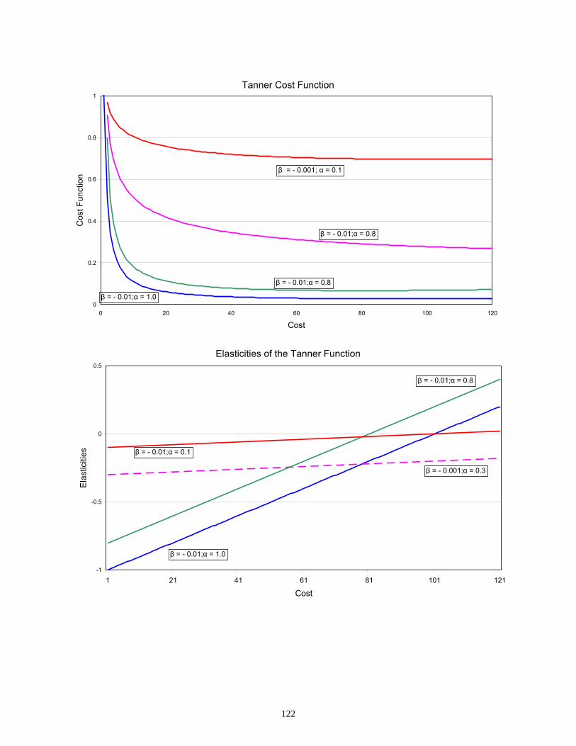
122

Tanner Cost Function

0

0.2

0.4

0.6

0.8

1

0 20 40 60 80 100 120

Cost

Cos

t Fun

ctio

n

β = - 0.01;α = 0.8

β = - 0.01;α = 1.0

β = - 0.001; α = 0.1

β = - 0.01;α = 0.8

Elasticities of the Tanner Function

-1

-0.5

0

0.5

1 21 41 61 81 101 121

Cost

Ela

stic

ities

β = - 0.001;α = 0.3

β = - 0.01;α = 0.8

β = - 0.01;α = 0.1

β = - 0.01;α = 1.0

123

EVA Cost Function(cost sensitivities b (beta) ranging from 0.001 to 1.0)

0

0.2

0.4

0.6

0.8

1

0 20 40 60 80 100 120

Cost

Cos

t Fun

ctio

n

b=0.001

b=0.01

b=0.1

b=1.0

Elasticities of the EVA Cost Function(cost sensitivities b (beta) ranging from 0.001 to 1.0)

-0.5

-0.4

-0.3

-0.2

-0.1

0

1 21 41 61 81 101

Cost

Ela

stic

ity

b=1.0

b=0.1

b=0.01

b=0.001

124

Exercises 1. Derivation of Balancing Factors Consider the following optimality condition from the derivation of the origin-destination choice model in Section 5.1: ( )pqmqppqm cd ⋅−+= µλκexp . Apply the following origin and destination constraints to this function, by substituting for pqmd .

∑∑

∑∑∈=

∈=

p mqpqm

pq m

pqm

QqDd

PpOd

,

;,

Write out the constraints without using summation signs, factor out common terms, and prove

that the following results are correct: ( ) ( ) ( )

( ) ( ) ( )∑ ⎟⎠⎞⎜

⎝⎛ ∑ ⋅−=

∑ ⎟⎠⎞⎜

⎝⎛ ∑ ⋅−=

p mpqmpqq

q mpqmqpp

cD

cO

µκλ

µλκ

expexpexp

expexpexp

2. Singly Constrained Trip Distribution Model The doubly-constrained model formulated in Section 5 is one of a family of O-D choice models. Another class of this family of models is the singly-constrained model. Consider the following scenario. Households choose their shopping locations on the basis of the size of shops, measured by floor area, and the generalized cost from their home to the shopping areas. The number of households per zone is given, as is the floor area per shopping zone Sq. Prior to consideration of travel costs, the expected number of trips per time period is proportional to Sq/P, where P is the number of residential zones. To represent the dispersion of trips given the prior information, we consider the following

generalized dispersion function: 0/ln S

PSd

dpq m q

pqpqm ≥∑∑ ⎟

⎟⎠

⎞⎜⎜⎝

⎛−

Assume that travel is constrained only by the trips per period leaving the origin zone p: PpOd p

qpq ∈=∑ ,

Formulate and solve a shopping location choice model for this situation. To simplify the derivation, you may assume that mode choice is not represented in the model. In other words, delete the subscript m. Discuss the relation of the resulting model to the logit model introduced in Section 4.

125

6. Combined Models and Feedback 6.1 Problem Statement It is unusual for the solution algorithm of a mathematical problem to be regulated by an Act of the U. S. Congress and a decree of a U. S. court resulting from a civil lawsuit. To a substantial extent, that is what has occurred with regard to the Congressional and judicial mandates to solve the four-step travel forecasting procedure “with feedback.” In particular, see the Intermodal Surface Transportation Efficiency Act of 1991. In these notes, we seek to understand the issue of feedback, and the related combined model of origin-destination, mode and route choice. After examining the basic concepts, we consider a combined model implementation and a recommended feedback procedure. The four-step procedure views the representation of the choice of where to travel, by what mode to travel, and by what route to travel as three separate, but loosely related choices which are dependent on travel times and costs prevailing in the highway and transit networks. The fourth dimension of travel choice, how often to travel, is generally regarded as independent of network conditions, and assumed to depend on traveler and household characteristics; accordingly, it will not be considered further here except as a source of control totals for the remaining travel choices. A principal difficulty with solving the sequential procedure is that the travel times and costs on the road network are not fixed and known, but rather are the result of solving an equilibrium model, as has been seen in our consideration of trip assignment (route choice) models. In the four-step procedure, however, these generalized travel costs are not just needed for the route choice model, but are also essential inputs to the O-D choice and mode choice models, known traditionally as trip distribution and mode split models. Since the solution of these models also determines the outcome of the route choice model, a circularity exists, which has come to be known in the urban transportation planning field as “solving the models with feedback.” Stated intuitively, the problem is to bring the generalized travel costs, which are inputs to the travel choice models and outputs of the route choice models, into agreement. There is at least one other difficulty, namely that the definitions of travel times and costs in the three choice models are not always consistent. For example, auto and transit travel times may be the basis for the route choice models, modal travel times and operating costs/fare the basis for the mode choice model, but only auto travel times the basis for the O-D choice model. While it is not imperative for these travel times and costs to be the same in each model, they should be defined consistently. This problem is as old as the four-step procedure itself. Moreover, it was the subject of considerable study in the early 1970s by a British applied mathematician, John D. Murchland, and an Australian graduate student at University College London, Suzanne P. Evans. She successfully solved the problem of “combining trip distribution and trip assignment” in her Ph.D. thesis completed in 1973, published two papers on her findings and left the field. A somewhat parallel effort by Michael Florian at the University of Montreal produced a related, but less

126

useful result. Because of the term coined by Murchland and Evans, these formulations came to be known as combined models. When the problem of “solving the four-step procedure with feedback” is viewed from the standpoint of “combined models”, we believe that the conceptual issues are at once clear and straightforward. However, our experience is that the combined model framework is not as compelling to others as it is to us. This situation inspires us to try again to communicate these results effectively. 6.2 Formulation of the Combined Model We begin our formulation with the auto route choice model with the objective function augmented to include transit costs:

( )( )

Aahf

QqPpdh

dcdxxcz

pqa

pq

a

Rr

arra

pqaRr

r

pqpqtpqt

a

f

a

∈≡

≥

===

⋅+⋅=

∑

∑

∑∑ ∫

∈

∈

, where

,...1;,...1,/ s.t.

)(min0

δ

η

η

0h

hh

where pqmd is given for each mode, and the auto occupancy η is given. To this objective function and route flow conservation constraint, we add constraints requiring that the auto and transit flows from zone p to zone q sum to the fixed O-D flows dpq. Then, we define a dispersion constraint that relates the dispersion of flows to the higher cost mode to the observed dispersion. Finally, we have constraints requiring all variables to be nonnegative.

.,,,...1;,...1,0

ln

,...1;,...1,

0

tamQqPpd

Sdd

QqPpddd

pqm

pqmpqmpqm

pqpqtpqa

===>

=−

===+

∑

In this formulation, we have relaxed some constraints on the auto route choice model, added a term in the objective function relating to transit costs, and added conservation of flow constraints pertaining to mode choice. The result is a combined mode and route choice model with the following properties: 1. The route choice conditions are similar to conditions in the UO route choice model; 2. The mode choice conditions correspond to the familiar logit model of mode choice:

127

( )( )∑

∈

⋅−

⋅−=

,expexp

tanpqn

pqmpqpqm c

cdd

µµ

where pqmc is the generalized travel cost of mode m, and pqac is the UO auto cost.

3. To add O-D choice to the model, we relax the constraint that pqd is fixed, and add the following constraints:

∑

∑==

==

pmqpqm

qmppqm

QqDd

PpOd

,...1,

,...1,

These constraints are the familiar row and column sum constraints from the O-D choice (trip distribution) model, which state that the origin-destination-mode flows must sum to the specified origin and destination totals.

4. The optimality conditions of this model are the same as before for route choice, plus ( )pqmqqpppqm cDBOAd ⋅−= µexp

where qp BA and are balancing factors that insure the origin and destination constraints are satisfied.

In summary, from this formulation, we can see that the way to combine O-D and mode choice with route choice is to augment the route choice problem with the constraints pertaining to O-D and mode choice. This was the first major insight of S. P. Evans. Her second fundamental result was to show that the Frank-Wolfe linearization method could be generalized to a partial linearization method to solve this problem formulation, and to prove that the algorithm does converge to the desired solution. The mathematical result is presented in detail in Patriksson (1994), as well as in Evans (1976). This algorithm is stated in the next section. 6.3 Evans Algorithm for the Combined Model The fundamental insight of Evans was to realize that it is only necessary to linearize that part of the objective function pertaining to variables which cannot be solved directly from the optimality conditions. Since optimality conditions are available that define origin-destination and mode choice, as described above, only the auto route choice portion of the objective function is linearized, as in the traffic assignment problem with fixed demand. Once the O-D-mode and route choice variables have been updated, then a line search is used to find a step length or weight to drive the solution towards the optimum. The problem to be solved by the algorithm may be stated as follows.

128

TAP-ODMC

( )( )

Aahf

QqPpRrh

tamQqPpd

QqDd

PpOd

QqPpddd

QqPpdh

dddcdxxcz

pqa

pq

a

Rr

arra

pqr

pqm

pmqpqm

qmppqm

pqpqtpqa

pqaRr

r

pqmpqmpqm

pqpqtpqt

a

f

a

∈∑≡

==∈≥

===>

∑ ==

∑ ==

===+

===∑

∑⋅+∑ ⋅+∑ ∫⋅=

∈

∈

, where

,...1;,...1,,0

,,,...1;,...1,0

,...1,

,...1,

,...1;,...1,

,...1;,...1,/ :st

ln1),(min0

δ

ηµ

ηhdhd,

The objective function has been augmented to include the only nonlinear term of the Lagrange function, ∑−

pqmpqmpqm dd ln , and its Lagrange multiplier µ/1 . All of the constraints are linear.

The main problem variables are the origin-destination-mode flows ( )pqmd and the auto link flows ( )af ; the subproblem variables are ( )pqme and ( )ag respectively. The Evans algorithm is stated as follows. 1. Initialization - compute an initial solution ( )1

pqmd , ( )1af for origin-destination-mode flows and

link flows; a common procedure is to set road link flows to zero, compute the links costs and the shortest route costs, solve for the O-D-mode flows, and assign the O-D auto flows to their shortest routes.

2. Update link costs: ( )k

aaa fcc = where the iteration index k is initially 1. 3. Compute shortest routes from each origin p to each destination q to obtain ( )k

pqac . 4. Solve the origin-destination-mode choice model for the subproblem flows ( )k

pqme . 5. Perform an all-or-nothing assignment of the auto O-D flows ( )k

pqae to the shortest routes from

p to q, yielding link flows ( )kag ; that is, increase the flow on each link of the shortest route by

the O-D-auto mode flow. 6. Compute the Relative Gap and test for convergence:

129

( ) ( ) ( ) ( ) ( )

( ) ( ) k

pqm

kpqm

kpqm

pqpqtpqt

a

f

ak

pqm

kpqm

kpqm

pqm

kpqm

kpqm

pq

kpqt

kpqtpqt

ka

ka

a

kaa

k

dddcdxxc

ddeedecfgfc

a

Gapln1LB

ln1ln1Gap

0

+++⋅=

−+−+−⋅⋅=

∑∑∑ ∫

∑∑∑∑

µη

µµη

( ) ( ) ( ) ( )

( ) ( ) ( )

( ) ( ) ( ) ( )∑∑∑∑ ∫

∑∑∑

∑∑∑∑ ∫

++−⋅⋅+⋅=

−+−+

−⋅⋅+++⋅=

pqm

kpqm

kpqm

pqpqtpqt

ka

ka

a

kaa

a

f

a

pqm

kpqm

kpqm

pqm

kpqm

kpqm

pq

kpqt

kpqtpqt

ka

ka

a

kaa

pqm

kpqm

kpqm

pqpqtpqt

a

f

a

eeecfgfcdxxc

ddeedec

fgfcdddcdxxc

a

a

ln1

ln1ln1

ln1

0

0

µηη

µµ

ηµ

η

( )

7. Step togo otherwise STOP; YES, If ?BLBGapGap Relative theIs

LBmaxBLB

ε<≡

=

kk

k

k

7. Perform a line search to determine the optimal step length (weight) kλ :

( ) ( ) ∑⋅+∑ ⋅+∑ ∫⋅= ++++

pqm

kpqm

kpqm

pq

kpqtpqt

a

f

ak dddcdxxcz

ka

k

111

0ln1)(min

1

µηλ

λ

where ( ) ka

kka

kka gff ⋅+⋅−=+ λλ11 and ( ) k

pqmkk

pqmkk

pqm edd ⋅+⋅−=+ λλ11 8. Update the O-D-mode and link flows:

( )( ) k

akk

akk

a

kpqm

kkpqm

kkpqm

gff

edd

⋅+⋅−=

⋅+⋅−=+

+

λλ

λλ

1

11

1

9. Retest the updated value of the objective function for convergence. The algorithm is illustrated by the following simplified flowchart.

130

A Generalized Evans Algorithm

Inputs: Zonal origins and destinations: O, D Road network; initial link costs c(1) Set an iteration index k = 0.

)k(),k( ge

Origin-destination-mode choice model: Set k = k+1; find )k(e for minimal OD-auto costs from ( )kc , and O, D.

Auto route choice: assign OD flows )k(e to minimal cost routes as

determined by ( )kc , yielding )k(g . (all-or-nothing assignment)

( )[ ]1k +fc

Find the weight ,1)k(0),k( ≤≤ λλ that minimizes )],1k(),1k([ ++ fdF where:

);k()k()k()]k(1[)1k( edd ⋅+⋅−=+ λλ ).k()k()k()]k(1[)1k( gff ⋅+⋅−=+ λλ

update d, f and k = k+1.

Check convergence of d and f; if the convergence criterion is met, STOP. Otherwise, return to OD choice.

d*, f* Yes

No

)k(e

Optional assignment iterations: assign auto OD flows )1k( +d to road network with F-W method to desired level of convergence yielding ( )1k~

+f in place of ( ).1k +f

131

Comments on the verbal statement of the algorithm: 1. Step 3 involves applying a shortest route algorithm to each origin node p.

2. Step 4 consists of solving an origin-destination-mode choice model using a doubly-

constrained gravity model with mode-specific costs. 3. Step 5 performs an all-or-nothing assignment of O-D flow by auto to the road network. 4. According to Lundgren and Patriksson (1998), the solution of the subproblem provides a

lower bound on the optimal value of ),( hdz . Feasible solutions to TAP-ODMC provide upper bounds on ),( hdz . The difference between the upper and lower bounds may be regarded as the Gap. The Gap/BLB defines a Relative Gap, which may be used to monitor convergence of the solution.

5. Step 7 finds the optimal step length kλ . 6. Step 8 updates the O-D-mode flows and the auto link flows. 6.4 Case Study – An Application of the Combined Model to the Chicago Region A research team led by Boyce and Bar-Gera (2003) applied a multiple-class version of the combined model to data for the Chicago region from the 1990 Census and household survey. TAP-CM

( ) ( ) ( )

( ) ( )

( ) ∑ ⎟⎟⎠

⎞⎜⎜⎝

⎛−⎟⎟⎠

⎞⎜⎜⎝

⎛⋅+∑ −⋅+

∑ ⎟⎟⎠

⎞⎜⎜⎝

⎛+⋅+⋅+⋅+∑ ⋅++

⋅⋅∑+∑ ⋅⋅+⋅⋅+∑ ∫≡

lpqmlpq

lpqml

pqmlllpq

lpq

lpqll

lpq

ltrpq

ltrpq

ltrpq

ll

ltrpq

lpaupp

lauppl

laupp

aupql

aupqlpq

l

l

laa

la

la

la

l

a

f

aa

dd

ddd

wktd

std

wdsfkfftTa

1lnµ

11lnη

1

γγγγγ

γγγ,min

8,7,6,5,

,4,,

,,3

420

νν

νν

νhd

.;,,

.,,

.;,,: ,

LlZqpdd

ZqpKh

LlZqpd

hst

m

lpq

lpqm

pqRr

kr

l

laupq

Rr

lr

pq

pq

∈∈=

∈=

∈∈=

∑

∑

∑

∈

∈ ν

.;,

.;,

LlZqDd

LlZpOd

lq

p

lpq

lp

q

lpq

∈∈=∑

∈∈=∑

132

.,,,0

.;,,,0

ZqpRrh

LlZqpRrh

pqkr

pqlr

∈∈≥

∈∈∈≥

.,δδwhere Aahhfffr

ar

kr

lr

ar

lr

l

ka

laa ∈∑+∑∑ ≡+≡

Additional definitions used in the above formulation are:

( ) =aa ft in-vehicle auto travel time on road link a, a function of total vehicle flow af (min)

ak = vehicle toll per auto equivalent unit on link a or parking fee at the terminal link (cents)

as = length of link a (miles) =a

rδ 1, if link a belongs to route r, and 0 otherwise =auppt , average in-vehicle auto travel time within zone p (minutes); fixed, exogenous value =aupps , average length of auto trip within zone p (miles); fixed, exogenous value =aupqw , out-of-vehicle travel time by auto for travel from zone p to zone q (minutes)

=trpqt , in-vehicle transit travel time from zone p to zone q (minutes) =trpqk , transit fare from zone p to zone q (cents) =trpqw , out-of-vehicle travel time by transit from zone p to zone q (minutes)

,1γ1 =l the coefficient associated with auto in-vehicle travel time for class l =l

2γ the coefficient associated with auto monetary cost for class l =l

3γ the coefficient associated with auto out-of-vehicle travel time for class l =l

4γ the coefficient associated with auto travel distance for class l =l

5γ the coefficient associated with transit in-vehicle travel time for class l =l

6γ the coefficient associated with transit fare for class l =l

7γ the coefficient associated with transit out-of-vehicle travel time for class l =l

8γ the coefficient associated with transit bias for class l =ll η,µ mode and OD cost sensitivity parameters for class l

The ODM choice model implied by this formulation is:

( ) ( )( )∑ −

−⋅−=

m

lpqm

l

lpqm

llpq

llq

lq

lp

lp

lpqm c

ccDBOAd

µexpµexp~ηexp

This model was estimated with data from the 1990 household travel survey (HHTS) conducted by the Chicago Area Transportation Study. Details of the estimation procedure are described by Boyce and Bar-Gera (2003). The convergence of the solution to the Chicago model is shown on the next two charts followed by two maps of the region and the model parameters and performance measures in Tables 1 and 2. For comparison with a model of a less congested region, results are also shown for Tucson, Arizona.

133

Convergence of Two Combined Models

-11.42

-11.41

-11.40

-11.39

-11.38

-11.37

-11.36

-11.35

-11.34

-11.33

1 2 3 4 5 6 7Iterations of the Evans Algorithm

Obj

. Fn.

and

BL

Boun

d - T

ucso

n

-140

-130

-120

-110

-100

-90

-80

-70

-60

-50

Obj

. Fn.

and

BL

Boun

d - C

hica

go

Objective Function - Tucson

Best Lower Bound - Tucson

Objective Function - Chicago

Best Lower Bound - Chicago

Relative Gaps and Step Sizes for Two Combined Models

1.E-04

1.E-03

1.E-02

1.E-01

1.E+00

1.E+01

1 2 3 4 5 6 7Iterations of the Evans Algorithm

Rel

ativ

e G

ap

0

0.1

0.2

0.3

0.4

0.5

Step

Siz

e

Relative Gap - Chicago

Relative Gap - Tucson

Step Size - Chicago

Step Size - Tucson

134

District and Zone Map for Chicago Region

Road Network Map for Chicago Region

TABLE 1: Estimated Values of Coefficients for Two Multiclass Travel Choice Models ____________________________________________________________________________

Travel Class Home-to-Work Travel Other Travel Generalized Cost Coefficients (units) Auto Transit Auto Transit

In-vehicle Travel Time (gc/min) 1.0 0.25 1.0 0.28 Out-of-vehicle Travel Time (gc/min) 0.0 0.90 0.47 0.46 Monetary Cost (gc/cents) 0.049 0.084 0.0003 0.052 Length of Route (gc/miles) 0.15 NA 0.05 NA Transit Bias (gc) NA 0.00 NA 0.09 Cost Sensitivity Coefficients Simultaneous O-D-Mode 0.14 0.25 Nested Logit O-D 0.13 0.28 Mode 0.15 0.20 Goodness-of-Fit

( )1ρ0 2 ≤≤

Simultaneous 0.19 0.33 Nested Logit 0.21 0.35

gc: generalized cost of travel in auto in-vehicle minutes NA: not applicable Note: All estimated values are rounded to two significant digits.

135

TABLE 2: Summary Means for the Multinomial Logit and Nested Logit Models ______________________________________________________________________________Class Home-to-Work Travel Mode Auto Transit Model Multi-Logit Nested Logit Multi-Logit Nested Logit Variable unit In-vehicle time minutes 16.1 17.7 25.5 24.9Out-of-vehicle time minutes 2.7 2.7 12.8 13.1Total travel time minutes 18.8 20.4 38.3 38.0Monetary cost dollars 0.31 0.34 1.46 1.46Length miles 10.8 11.5 NA NAGeneralized cost minutes 20.1 21.3 30.0 30.2Observed gen. cost minutes 18.4 18.6 29.7 29.7Regional share percent 83.7 83.7 16.3 16.3Observed reg.share percent 83.8 16.2 Central Area share percent 34.8 35.0 65.2 65.0Observed CA share percent 36. 64.

Class Other Travel Mode Auto Transit Model Multi-Logit Nested Logit Multi-Logit Nested Logit Variable unit In-vehicle time minutes 8.9 8.4 16.3 14.5Out-of-vehicle time minutes 2.5 2.6 15.5 14.0Total travel time minutes 11.3 10.9 31.9 28.5Monetary cost dollars 0.15 0.14 1.32 1.28Length miles 5.4 4.9 NA NAGeneralized cost minutes 11.8 11.2 18.6 17.2Observed gen. cost minutes 10.3 10.4 18.9 18.9Regional share percent 82.7 83.0 17.3 17.0Observed reg.share percent 82.8 17.2 Central Area share percent 40.8 51.3 59.2 48.7Observed CA share percent 41. 59.

NA – not applicable Italicized rows denote observed values. Observed generalized costs are different for the Simultaneous and Nested Logit models because of differences in model coefficients that determine these values.

The Evans algorithm was used in the estimation procedure, as well as for solving the final model for validation studies. The validation studies are shown in the following figures. The first four figures for Home-to-Work Travel compare the Census validation data and the model predictions aggregated by airline distance from origins to destinations. The data on which the model was estimated is also shown. The following four figures for Other Travel show only the predictions and the data used in the estimation, since Census data are not available for this class of travel. The last two sets of figures compare the predictions and Census data for district-to-district flows.

136

OD Proportion vs. Airline Distance Home-to-Work Travel by Auto and Transit

0.001

0.01

0.1

0 10 20 30Airline Distance (miles)

OD

Pro

porti

on

Model

Census

HHTS

0.012

0.038

0.028

Transit Share vs. Airline DistanceHome-to-Work Travel

0.01

0.1

1

0 10 20 30

Airline Distance (miles)

Tran

sit S

hare

Model - 0.178

Census - 0.175

HHTS - 0.179

Series Regional Share

0.178

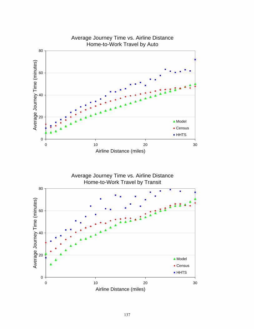
137

Average Journey Time vs. Airline Distance Home-to-Work Travel by Auto

0

20

40

60

80

0 10 20 30

Airline Distance (miles)

Ave

rage

Jou

rney

Tim

e (m

inut

es)

Model

Census

HHTS

Average Journey Time vs. Airline Distance Home-to-Work Travel by Transit

0

20

40

60

80

0 10 20 30

Airline Distance (miles)

Ave

rage

Jou

rney

Tim

e (m

inut

es)

Model

Census

HHTS

138

OD Proportion vs. Airline Distance Other Travel by Auto and Transit

0.00001

0.0001

0.001

0.01

0.1

1

0 10 20 30

Airline Distance (miles)

OD

Pro

porti

on

Model

HHTS

0.053

0.199

Transit Share vs. Airline Distance Other Travel

0.001

0.01

0.1

1

0 10 20 30

Airline Distance (miles)

Tran

sit S

hare

Model - 0.189

HHTS - 0.069

Series Regional Share

0.189

139

Average Journey Time vs. Airline Distance Other Travel by Auto

0

20

40

60

80

0 10 20 30

Airline Distance (miles)

Aver

age

Jour

ney

Tim

e (m

inut

es)

Model

HHTS

Average Journey Time vs. Airline Distance Other Travel by Transit

0

20

40

60

80

0 10 20 30

Airline Distance (miles)

Ave

rage

Jou

rney

Tim

e (m

inut

es)

Model

HHTS

140

Ratio of Census O-D Proportions to Model O-D Proportions vs. Model O-D Proportions

0.10

1.00

10.00

100.00

1000.00

1E-07 1E-06 0.00001 0.0001 0.001 0.01 0.1 1

OD Proportion (model)

Rat

io

C. A.N. ChicagoW. ChicagoS. ChicagoN. CookW. CookS. CookDuPageLake ILKaneMcHenryWill

Origin

0.10

1.00

10.00

100.00

1000.00

1E-07 1E-06 0.00001 0.0001 0.001 0.01 0.1 1

OD Proportion (model)

Rat

io

C. A.N. ChicagoW. ChicagoS. ChicagoN. CookW. CookS. CookDuPageLake ILKaneMcHenryWill

141

Census O-D Proportions Less Model O-D Proportions vs. Model O-D Proportions

-0.02

-0.015

-0.01

-0.005

0

0.005

0.01

0.015

0.02

1E-07 1E-06 0.00001 0.0001 0.001 0.01 0.1 1

OD Proportion (model)

Diff

eren

c

C. A.N. ChicagoW. ChicagoS. ChicagoN. CookW. CookS. CookDuPageLake ILKaneMcHenryWill

Origin

-0.02

-0.015

-0.01

-0.005

0

0.005

0.01

0.015

0.02

1E-07 1E-06 0.00001 0.0001 0.001 0.01 0.1 1

OD Proportion (model)

Diff

eren

c

C. A.N. ChicagoW. ChicagoS. ChicagoN. CookW. CookS. CookDuPageLake ILKaneMcHenryWill

Destination

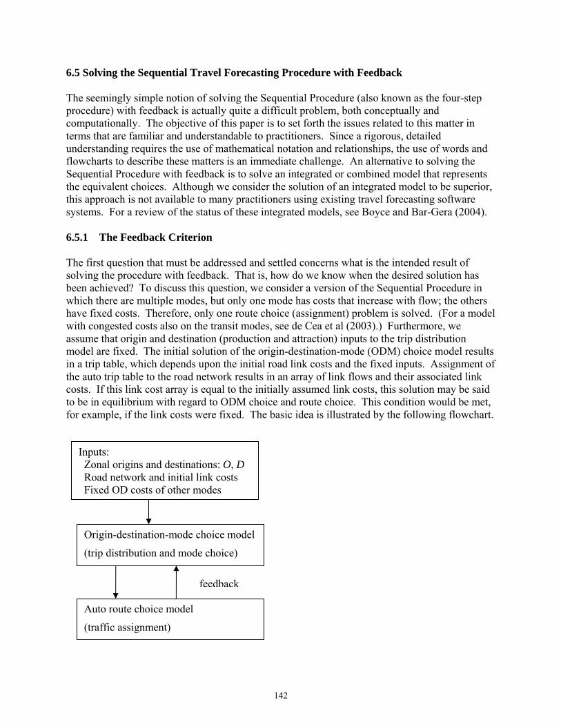
142

6.5 Solving the Sequential Travel Forecasting Procedure with Feedback The seemingly simple notion of solving the Sequential Procedure (also known as the four-step procedure) with feedback is actually quite a difficult problem, both conceptually and computationally. The objective of this paper is to set forth the issues related to this matter in terms that are familiar and understandable to practitioners. Since a rigorous, detailed understanding requires the use of mathematical notation and relationships, the use of words and flowcharts to describe these matters is an immediate challenge. An alternative to solving the Sequential Procedure with feedback is to solve an integrated or combined model that represents the equivalent choices. Although we consider the solution of an integrated model to be superior, this approach is not available to many practitioners using existing travel forecasting software systems. For a review of the status of these integrated models, see Boyce and Bar-Gera (2004). 6.5.1 The Feedback Criterion The first question that must be addressed and settled concerns what is the intended result of solving the procedure with feedback. That is, how do we know when the desired solution has been achieved? To discuss this question, we consider a version of the Sequential Procedure in which there are multiple modes, but only one mode has costs that increase with flow; the others have fixed costs. Therefore, only one route choice (assignment) problem is solved. (For a model with congested costs also on the transit modes, see de Cea et al (2003).) Furthermore, we assume that origin and destination (production and attraction) inputs to the trip distribution model are fixed. The initial solution of the origin-destination-mode (ODM) choice model results in a trip table, which depends upon the initial road link costs and the fixed inputs. Assignment of the auto trip table to the road network results in an array of link flows and their associated link costs. If this link cost array is equal to the initially assumed link costs, this solution may be said to be in equilibrium with regard to ODM choice and route choice. This condition would be met, for example, if the link costs were fixed. The basic idea is illustrated by the following flowchart.

Origin-destination-mode choice model

(trip distribution and mode choice)

Auto route choice model

(traffic assignment)

feedback

Inputs: Zonal origins and destinations: O, D Road network and initial link costs Fixed OD costs of other modes

143

Although the above statement may be considered to be acceptable, it does contain an implicit assumption, namely that the origin-destination-auto costs can be determined from the link costs. One way in which these costs can be determined is to assume that origin-destination costs are equal to the costs of minimal cost routes. As we shall see later, other possibilities might be assumed. If we assume in addition that the initial link costs are based on zero link flows, then minimal cost routes would be suitable, since there are no route flows in the network. Assuming that the equality of link costs is not immediately satisfied, we require a condition that is independent of the initially assumed link costs. Two ways to state this condition are: 1. The usual procedure is to assume that the trip table is determined by an array of road link costs c(f), which depends on a link flow array f. If this trip table is assigned to the road network by an unspecified method, and results in link flows f with costs ( )fc ˆ that are equal to those on which the trip table was based, ( )fc , then we can say that this Sequential Procedure is in equilibrium. 2. A more general statement would include the solution of the ODM choice step as well as the traffic assignment step. Suppose the ODM choice step depends on arrays of previously derived link flows, which in an unspecified manner, produces a trip table d. Suppose that trip table d is assigned to the road network by an unspecified method, resulting in a link flow array, and we use that array and the ODM choice model to produce a new trip table d , which depends directly on that array, as well as other fixed inputs common to both trip tables. We can now ask whether these two trip tables, d and d , are equal. If they are, then the Sequential Procedure is in equilibrium. In this second case, we have also not made any assumption about how either model is solved. However, we do claim that if the equilibrium link flow array can produce a trip table equal to the current trip table, then we have found an equilibrium solution. We return to this question in 6.5.7. As a result of these two statements, we now have an understanding of what criteria must be satisfied to achieve the condition that is generally called, “solving the Sequential Procedure with feedback.” Next we consider procedures for generating trip tables and link flow arrays that satisfy these conditions. 6.5.2 Types of Feedback Several ways to solve the Sequential Procedure with feedback have been defined and applied. We categorize them generally as follows: 1. Procedures that do not involve averaging of either trip tables or link flow arrays. For short,

we describe these as naïve feedback methods, without intending to be pejorative. 2. Procedures based on the formulation of the Sequential Procedure as a convex programming

problem or a fixed point problem. In these special cases, algorithms can be constructed and their convergence to satisfy the above criterion proved. Examples are algorithms proposed by Evans (1976) and Bar-Gera and Boyce (2003).

144

3. In cases in which a convex programming problem is not known to exist, one can appeal to methods related to optimization problems, and apply the Method of Successive Averages (MSA) or even Constant Weights.

6.5.3 A Naïve Feedback Procedure Discussions with numerous practitioners regarding how they solve the Sequential Procedure with feedback led to the following statement, as represented in Fig. 1: 1. Solve the ODM choice model by using an array of initial link costs c(0) = c[f(0)] to

determine the costs of the minimal cost routes, resulting in the trip table d(1); the initial link flows f(0) are often assumed to be zero.

2. Assign trip table d(1) to the road network, resulting in link flows f(1). Compute the link

costs c(1) = c[f(1)] that depend upon f(1), and solve for the minimal cost routes. 3. Using the link cost array c(1), re-solve the ODM choice model and re-assign the auto part of

the resulting trip table d(2) to the road network, resulting in f(2) and c[f(2)]. In some variants, link speeds are used in place of link costs; moreover, costs or speeds from successive feedback loops are sometimes averaged in an attempt to dampen oscillations.

4. Repeat step 3 a predetermined number of times n. The final trip table d(n) and link flow

array f(n) are the answer to the Sequential Procedure. What conclusions can one draw about this feedback procedure? First, since the final result depends upon congested link flows and link costs, it is likely to be preferred to the initial solution based on the assumed link flows. Second, the procedure does not invoke any test to determine whether the final trip table d(n) is in equilibrium with the final link costs c(n), so one cannot claim that the procedure has reached equilibrium. Third, what one can conclude is that the ODM choice and route choice models have been solved several times with different assumptions about the input link flow array, f(0), f(1), f(2), … f(n-1)? One cannot conclude anything about the validity of these assumptions, or about the equilibrium solution. 6.5.4 Procedures Based on Integrated (or Combined) Optimization Formulations The first successful attempt to devise a travel forecasting model, by Martin Beckmann and his co-authors (1956), proposed a single, rather general model of origin-destination choice and route choice. That is, they did not propose to solve a sequence of models, but included both OD choices and route choices over the network in a single, integrated model. Beckmann did not devise a way to solve the model; indeed, he has stated that he never imagined that it would be solved for large networks and zone systems (Boyce, 2004). His model was so advanced for its time that virtually no one understood its significance. Nearly 20 years passed before a connection was identified between Beckmann’s formulation and the Sequential Procedure devised by early practitioners about the same time. The person who noticed this connection most clearly was Suzanne Evans in her 1973 Ph.D. thesis; she devised a

145

procedure for solving the problem, called an algorithm, which has since been shown to be somewhat practical for large networks (Boyce and Bar-Gera, 2003, 2004). By then, however, the Sequential Procedure was so ingrained in the thinking of both academics and practitioners that hardly anyone noticed that Beckmann’s model, and its descendents, could now be solved. From the vantage point of formulation of Beckmann and the algorithm of Evans, the answer to the feedback question is immediately apparent. But first, one should try to understand the implications of his formulation. The unknown variables of the formulation are trip tables d and link flow arrays f, just as in the above representation of the Sequential Procedure. Beckmann’s formulation was stated as a constrained optimization problem, which simply means the minimization of a function of d and f, subject to some definitional constraints. Let us denote this function as F(d, f), which we assume to be convex, meaning that it is generally U-shaped and therefore has a unique minimum. The definitional constraints are that the OD-auto flow equals the sum of the route flows for each OD pair, and that the route flows are greater than or equal to zero. Through the analysis of this problem, one learns some facts about the conditions that describe the desired equilibrium, where “e” following a variable symbol in parentheses denotes the optimal, or equilibrium, solution: 1. The equilibrium trip table d(e) is determined by the ODM choice model based on link costs

c(e), determined by the equilibrium link flows f(e), as well as the given zonal origins and destinations, O and D, assuming the functional form of the model corresponds to this framework. The primary candidates in this regard are the several variants of the logit model. Thus, the solution of Beckmann’s formulation contains the statement of the equilibrium condition for ODM choices, which the Sequential Procedure is intended to fulfill.

2. The equilibrium route choices that determine f(e) have the user-equilibrium properties often

attributed to Wardrop, which were independently described and investigated by Beckmann:

Origin-destination-mode choice model

(trip distribution and mode choice)

Auto route choice model

(traffic assignment)

c[f(k)]

Inputs: Zonal origins and destinations: O, D Road network; initial link costs: c(0) Fixed OD costs of other modes

d(k)

Fig. 1 A Naïve Feedback Procedure

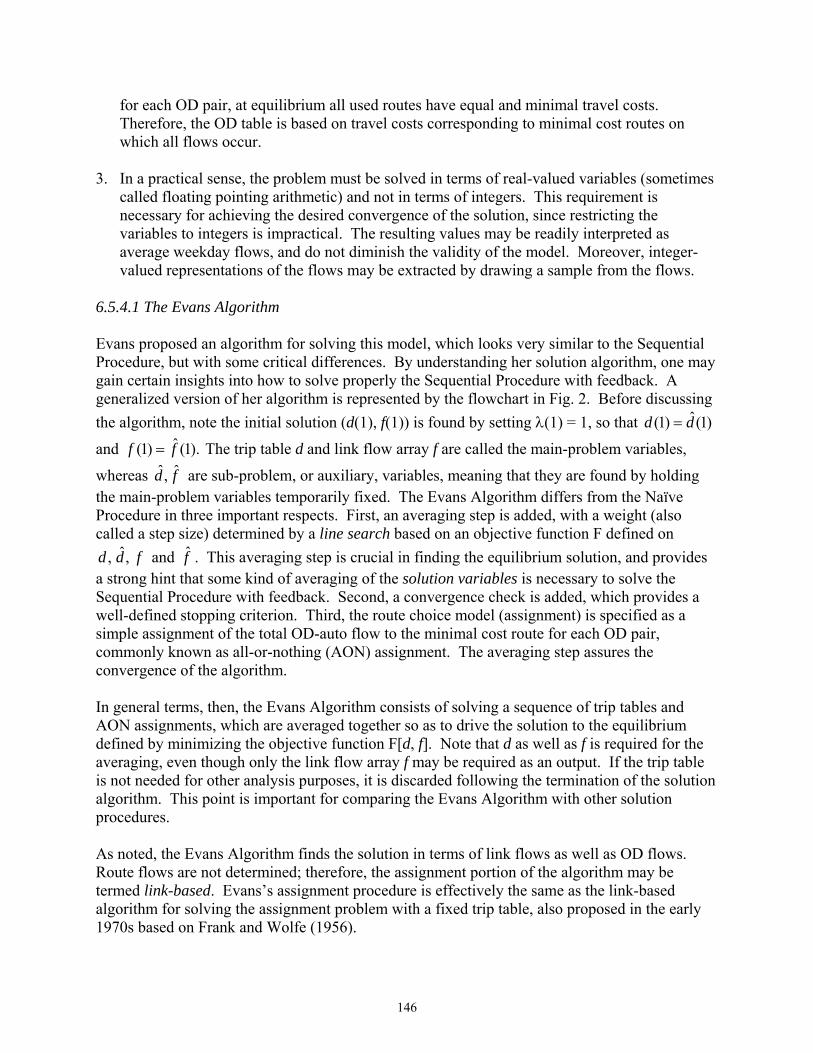
146

for each OD pair, at equilibrium all used routes have equal and minimal travel costs. Therefore, the OD table is based on travel costs corresponding to minimal cost routes on which all flows occur.

3. In a practical sense, the problem must be solved in terms of real-valued variables (sometimes

called floating pointing arithmetic) and not in terms of integers. This requirement is necessary for achieving the desired convergence of the solution, since restricting the variables to integers is impractical. The resulting values may be readily interpreted as average weekday flows, and do not diminish the validity of the model. Moreover, integer-valued representations of the flows may be extracted by drawing a sample from the flows.

6.5.4.1 The Evans Algorithm Evans proposed an algorithm for solving this model, which looks very similar to the Sequential Procedure, but with some critical differences. By understanding her solution algorithm, one may gain certain insights into how to solve properly the Sequential Procedure with feedback. A generalized version of her algorithm is represented by the flowchart in Fig. 2. Before discussing the algorithm, note the initial solution (d(1), f(1)) is found by setting λ(1) = 1, so that )1(ˆ)1( dd =

and ).1(ˆ)1( ff = The trip table d and link flow array f are called the main-problem variables,

whereas fd ˆ,ˆ are sub-problem, or auxiliary, variables, meaning that they are found by holding the main-problem variables temporarily fixed. The Evans Algorithm differs from the Naïve Procedure in three important respects. First, an averaging step is added, with a weight (also called a step size) determined by a line search based on an objective function F defined on

fdd ,ˆ, and f . This averaging step is crucial in finding the equilibrium solution, and provides a strong hint that some kind of averaging of the solution variables is necessary to solve the Sequential Procedure with feedback. Second, a convergence check is added, which provides a well-defined stopping criterion. Third, the route choice model (assignment) is specified as a simple assignment of the total OD-auto flow to the minimal cost route for each OD pair, commonly known as all-or-nothing (AON) assignment. The averaging step assures the convergence of the algorithm. In general terms, then, the Evans Algorithm consists of solving a sequence of trip tables and AON assignments, which are averaged together so as to drive the solution to the equilibrium defined by minimizing the objective function F[d, f]. Note that d as well as f is required for the averaging, even though only the link flow array f may be required as an output. If the trip table is not needed for other analysis purposes, it is discarded following the termination of the solution algorithm. This point is important for comparing the Evans Algorithm with other solution procedures. As noted, the Evans Algorithm finds the solution in terms of link flows as well as OD flows. Route flows are not determined; therefore, the assignment portion of the algorithm may be termed link-based. Evans’s assignment procedure is effectively the same as the link-based algorithm for solving the assignment problem with a fixed trip table, also proposed in the early 1970s based on Frank and Wolfe (1956).

147

Fig. 2 A Generalized Evans Algorithm

( )[ ]1k +fc )k(d

Inputs: Zonal origins and destinations: O, D Road network; initial link costs c(0) Set a loop index k = 1.

)k(ˆ),k(ˆ fd

Origin-destination-mode choice model: Set k = k+1; find )k(d for minimal OD-auto costs from ( )kc , and O, D.

Auto route choice: assign OD flows )k(d to minimal cost routes as

determined by ( )kc , yielding )k(f . (all-or-nothing assignment)

Find the weight ,1)k(0),k( ≤≤ λλ that minimizes )],1k(),1k([ ++ fdF where:

);k(ˆ)k()k()]k(1[)1k( ddd ⋅+⋅−=+ λλ

).k(ˆ)k()k()]k(1[)1k( fff ⋅+⋅−=+ λλupdate d, f and k = k+1.

Check convergence of d and f; if the convergence criterion is met, STOP. Otherwise, return to OD choice. d(e), f(e)

Yes

No

Optional assignment iterations: assign auto OD flows )1k( +d to road network with F-W method to desired level of convergence yielding ( )1k~

+f in place of ( ).1k +f

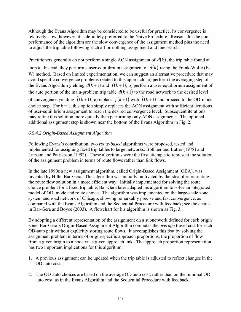
148

Although the Evans Algorithm may be considered to be useful for practice, its convergence is relatively slow; however, it is definitely preferred to the Naïve Procedure. Reasons for the poor performance of the algorithm are the slow convergence of the assignment method plus the need to adjust the trip table following each all-or-nothing assignment and line search. Practitioners generally do not perform a single AON assignment of ( )kd , the trip table found at

loop k. Instead, they perform a user-equilibrium assignment of ( )kd using the Frank-Wolfe (F-W) method. Based on limited experimentation, we can suggest an alternative procedure that may avoid specific convergence problems related to this approach: a) perform the averaging step of the Evans Algorithm yielding ( )1+kd and ( )1+kf ; b) perform a user-equilibrium assignment of the auto portion of the main-problem trip table ( )1+kd to the road network to the desired level of convergence yielding ( )1~

+kf ; c) replace ( )1+kf with ( )1~+kf and proceed to the OD-mode

choice step. For k = 1, this option simply replaces the AON assignment with sufficient iterations of user-equilibrium assignment to reach the desired convergence level. Subsequent iterations may refine this solution more quickly than performing only AON assignments. The optional additional assignment step is shown near the bottom of the Evans Algorithm in Fig. 2. 6.5.4.2 Origin-Based Assignment Algorithm Following Evans’s contribution, two route-based algorithms were proposed, tested and implemented for assigning fixed trip tables to large networks: Bothner and Lutter (1978) and Larsson and Patriksson (1992). These algorithms were the first attempts to represent the solution of the assignment problem in terms of route flows rather than link flows. In the late 1990s a new assignment algorithm, called Origin-Based Assignment (OBA), was invented by Hillel Bar-Gera. This algorithm was initially motivated by the idea of representing the route flow solution in a more efficient way. Initially implemented for solving the route choice problem for a fixed trip table, Bar-Gera later adapted his algorithm to solve an integrated model of OD, mode and route choice. The algorithm was implemented on the large-scale zone system and road network of Chicago, showing remarkably precise and fast convergence, as compared with the Evans Algorithm and the Sequential Procedure with feedback; see the charts in Bar-Gera and Boyce (2003). A flowchart for his algorithm is shown as Fig. 3. By adopting a different representation of the assignment on a subnetwork defined for each origin zone, Bar-Gera’s Origin-Based Assignment Algorithm computes the average travel cost for each OD-auto pair without explicitly storing route flows. It accomplishes this feat by solving the assignment problem in terms of origin-specific approach proportions, the proportion of flow from a given origin to a node via a given approach link. The approach proportion representation has two important implications for this algorithm: 1. A previous assignment can be updated when the trip table is adjusted to reflect changes in the

OD auto costs; 2. The OD-auto choices are based on the average OD auto cost, rather than on the minimal OD

auto cost, as in the Evans Algorithm and the Sequential Procedure with feedback.

149

No

( ) )1k(,1 ++ fkd

Inputs: Zonal origins and destinations: O, D Road network; initial link costs c(0) Initialize d(0) based on c(0), f(0) and

)0(γ with an all-or-nothing assignment. Set a loop index k = 0.

ODM choices: Set k = k+1; find )k(d for average OD-auto costs.

Find the weight ,1)k(0),k( ≤≤ λλ that minimizes )],k(),1k([ γ+dF where:

);k(ˆ)k()k()]k(1[)1k( ddd ⋅+⋅−=+ λλ

Check convergence of d and γ ; if convergence criteria are met, STOP. If not, return to OD and route choice.

Fig. 3 The Origin-Based Assignment Algorithm for an Integrated Travel Choice Model

d(e), f(e)

( ) )1k(,1k ++ γd

Yes

Auto route choice: update origin-based approach proportions to adjust the updated route flows to minimal cost routes, yielding 1).(k and )1k( ++ fγ

)k(d

( )1k +d

150

These advantages not only permit the algorithm to converge faster, but allows it to approach much closer to the true equilibrium. These advantages may also be true for some route-based algorithms, depending upon how they are implemented. The solution procedure is initialized by finding the trip table d based on the assumed link costs. The trip table is then assigned so as to place all OD-auto flows on user-equilibrium routes of equal and minimal cost, initially in an approximate manner. Based on this initial assignment and its associated OD-auto costs, the ODM choice function is applied to update the trip table, holding fixed the route proportions ( )kγ . Thus the computation of ( ) ( )kkd λ,ˆ and )1( +kd are based on ( )kγ . After this update is completed, new route proportions are determined. During the update

of route proportions from ( )kγ to ( )1+kγ , )1( +kd is held fixed. Several important distinctions between the Origin-Based Assignment Algorithm and the Evans Algorithm should be noted. First, the solution proceeds by refining the trip table and the associated route proportions. The link flows do not enter into the computations, except in determining the link costs. Second, the auto route proportions replace the auto link flows as the principal variable representing flows on the network. Because these are stored implicitly and compactly as origin-based approach proportions, the algorithm quickly reaches a precise solution, as compared with procedures based on link flows. 6.5.4.3 Monitoring the Convergence The description of the Evans and Origin-Based Assignment Algorithms is incomplete without specifying the convergence criteria. Although the criteria are related for the two algorithms, they are somewhat different. Moreover, the definitions for these algorithms provide guidance for monitoring the convergence of related procedures. Two convergence criteria are needed, one for the trip table and another for the link flow array. These criteria are often combined into a single criterion called the Relative Gap. Feasible solutions to convex optimization problems have an associated Lower Bound, which is defined on

ffd ˆ and ,ˆ for the Evans Algorithm and γγ ˆ and ,d for the Origin-Based Assignment Algorithm. The Relative Gap (RG) is formed from the lowest objective function value (LOF), which is always from the current loop, and the Best Lower Bound (BLB), which may be from a previous loop: ( ) BLBBLBLOFRG /−= . Because this paper does not provide details in equation form, the specification here is limited to verbal descriptions. Detailed specifications may be found in Bar-Gera and Boyce (2003). The Lower Bound contains terms related to the above variables, which can be given an intuitive interpretation. For the trip table variable, the Objective Function and Lower Bound corresponding to the logit function contain entropy terms defined on the trip table. For the trip table, we consider a simple criterion alluded to at the outset of the paper. This criterion is the Total Misplaced Flow, which is the sum of the absolute differences of zone-to-zone ODM flows in the main problem and subproblem solutions, .ˆ and dd If these two tables are equal, then the algorithm has converged with regard to the trip table.

151

For the route and link flow portion of the problem, we begin with a statement based on the intuitive notion of the Total Excess Cost. As noted, at user-equilibrium all used routes have equal and minimal travel cost. Therefore, there is no excess cost in the network in the sense that for each OD pair, no used route has a higher cost than the minimal cost route. For non-equilibrium solutions, however, flows with excess costs are present on some routes. Therefore, for each OD pair, we determine the difference between each used route’s cost and the minimal cost, weighted by the used route flow, and sum over all used routes for that OD pair to obtain the OD-auto excess cost. If we sum this quantity for all OD pairs, then we obtain the Total Excess Cost in the network. This quantity is directly computed by the Origin-Based Assignment Algorithm, as well as route-based algorithms. Remarkably, it can also be computed for any feasible link-based flow solution as well. To do so, one computes the link travel costs associated with the feasible link flow solution, and performs an all-or-nothing assignment, given these costs. The total travel cost of these two solutions may be computed separately by multiplying each link flow times the link cost, and summing over all links. The total cost of the feasible solution less the total cost of the all-or-nothing solution, evaluated as stated, is the Total Excess Cost. At equilibrium, the Total Excess Cost equals zero because the minimal OD costs in the all-or-nothing solution are the same as the equal and minimal route costs in the equilibrium solution. These two criteria, one for trip tables and one for link flows, provide intuitive and useful measures for evaluating any feasible solution, that is any solution that satisfies the origin inflows and destination outflows, as well as that the sum of route flows equal OD-auto flows for each OD pair. To my knowledge, these criteria are not generally applied by practitioners. 6.5.5 Procedures for Integrated Models Not Having an Optimization Formulation The above explanation is well and good for the limited case of formulations with an equivalent convex optimization formulation. But what about other formulations, and especially procedures applied in practice? For about 25 years it has been generally understood that the weights yielded by the line search step of the above algorithms can be replaced by predetermined weights, based on the properties of the Method of Successive Averages (MSA). This method becomes useful when no objective function F(d, f) is available. The weights ( )kλ generally applied with MSA are 1/k, where k is the loop number. The sequence of sub-problem weights generated by this method, then, are 1, 1/2, 1/3, 1/4, 1/5, … . The application of this sequence can be proven to converge to the equilibrium solution, but the convergence may be quite slow. Recent computational experiences revealed that using a Constant Weight instead of the decreasing weights of MSA may yield a substantially improved result (Bar-Gera and Boyce, 2006). In this case, the values of (1/k) in Fig. 4 are replaced by a constant weight between 0 and 1; typically a value near 0.5 was found to work well, but a range of weights should be tried to determine the best one for a given network and scenario. In the experiments reported in the next section, both MSA weights and Constant Weights were applied.

152

A flowchart illustrating this procedure for link-based, route-based and origin-based user-equilibrium assignment is shown as Fig. 4. In this procedure, only the successive trip tables are averaged with the MSA weights, and the resulting auto trip tables are assigned to the road network to determine the link flows and minimal or average OD auto travel costs needed for feedback. In this scheme, convergence of the feedback procedure is checked with the trip table only; convergence of assignments is checked at the assignment step within each feedback loop. 6.5.6 Findings of Preliminary Computational Experiments Computational experiments to compare Naïve Feedback, and feedback with the Method of Successive Averages and Constant Weights were performed with a model implemented by Wolfgang Scherr, PTV America, from the Capital District Transportation Committee, Albany, NY, in the PTV software system VISUM. The model has five classes of travelers with a total peak period OD flow of 313,082 persons per hour. The Sequential Procedure for this model was solved using the Naïve Feedback procedure, with a Relative Gap (convergence level) for the Assignment step of 0.0001. The model was also solved using the procedure described in Section 6.5.5 for models not having an optimization formulation. Two solutions were obtained, one using the Method of Successive Averages, and the other using a Constant Weight (CW) equal to 0.6 for d and 0.4 for d . In both cases, the convergence of the Assignment step was set to 0.0001. The convergence of the three solution methods were compared using the procedure defined in Section 6.5.4.3, Monitoring the Convergence, for the Total Misplaced Flow. Each assignment converged to a Relative Gap of slightly less than 0.0001; therefore, it is not useful to monitor its convergence. However, the number of assignment iterations needed to reach this Relative Gap varied substantially between the Naïve method and the other two methods. Total Misplaced OD Flows for the three solutions are shown in Fig. 5 using the log scale to facilitate their comparison. For Naïve Feedback, TMF reached a minimum value of 34,200 persons/hour in the 7th loop, which shows a large discrepancy between the trip table in the previous feedback loop and the trip table computed based on the travel times resulting from assigning that table in the current loop. At full convergence, TMF must equal zero, which means that a link flow array has been found whose minimum route generalized travel costs produce a trip matrix equal to the trip table that yielded those links flows. A value of zero persons/hour was achieved by the Constant Weight (CW) method in the 17th loop, and a value of less than 100 was reached in the 8th loop. The MSA method reached a minimum TMF of 127 persons/hour in the 20th loop when the process was terminated. The values are acceptably small for the MSA and CW methods. The number of assignment iterations in each loop required to achieve a Relative Gap of less than 0.0001 is shown in Fig. 6. For Naïve Feedback, the number of assignment iterations falls to 12 in loop 6, but then increases gradually to 27. For the other two methods, the number of assignment iterations falls rapidly to the minimum number of 2. In the route-based assignment algorithm applied in VISUM, the assignment is updated following the revision of the OD table. If a link-based method were used, then a new assignment solution is required in each feedback loop.

153

Inputs: Zonal origins and destinations: O, D Road network; initial link costs c(1) Set a loop index k = 0.

Origin-destination-mode choice model: set k = k+1; find )k(d for OD auto costs determined from ( )kc , O, D.

Determine: [ ] );k(ˆk/1)k(]k/11[)1k( ddd ⋅+⋅−=+

Check convergence of d; if the convergence criterion is met, STOP. Otherwise, return to OD choice.

d(e), f(e)

Auto route choice: assign )1k( +d to the road network to the desired level of convergence, yielding ( )1k +f .

Fig. 4 Feedback Procedure with Fixed Weights

minimal OD costs for link-based assignment; average OD costs for route-based assignment.

)1k( +d

)k(d

)1k(),1k( ++ fd

Yes

No

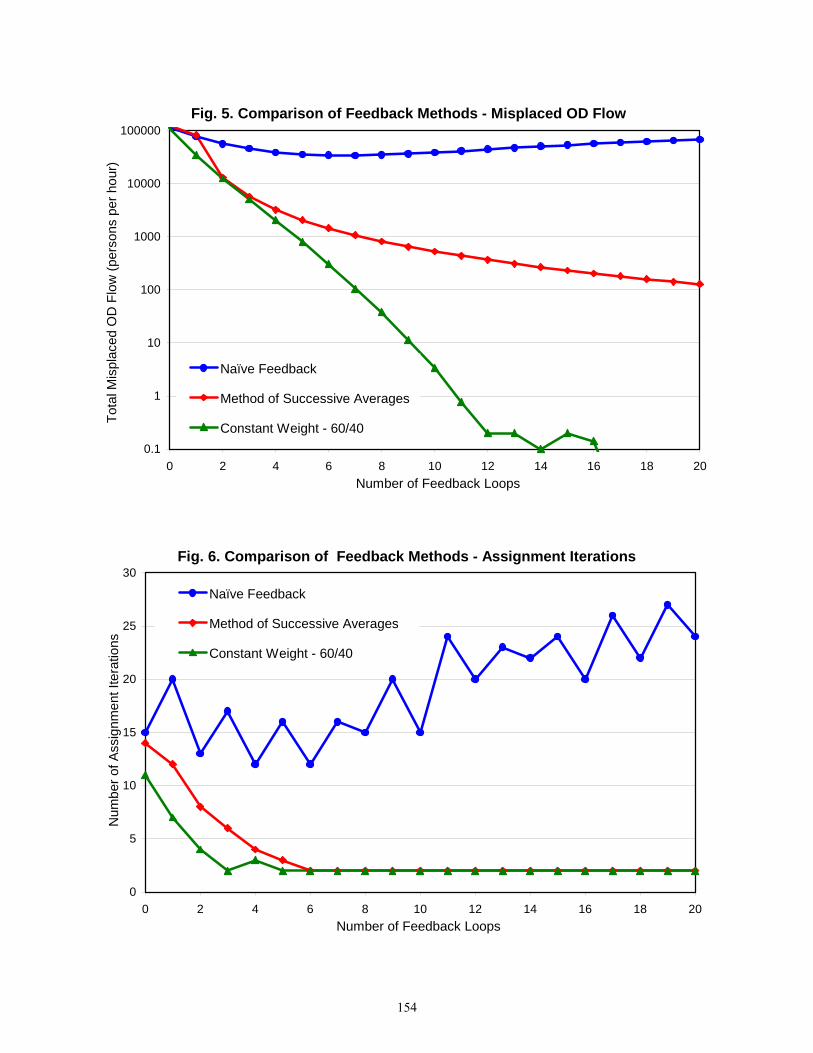
154

Fig. 5. Comparison of Feedback Methods - Misplaced OD Flow

0.1

1

10

100

1000

10000

100000

0 2 4 6 8 10 12 14 16 18 20Number of Feedback Loops

Tota

l Mis

plac

ed O

D F

low

(per

sons

per

hou

r)

Naïve Feedback

Method of Successive Averages

Constant Weight - 60/40

Fig. 6. Comparison of Feedback Methods - Assignment Iterations

0

5

10

15

20

25

30

0 2 4 6 8 10 12 14 16 18 20Number of Feedback Loops

Num

ber o

f Ass

ignm

ent I

tera

tions

Naïve Feedback

Method of Successive Averages

Constant Weight - 60/40

155

These results, as well as the extensive studies of the convergence of integrated models cited above, show that forecasts of origin-destination flows and link flows depend upon solving the sequential procedure properly with respect to travel times. In congested cities with several interacting modes, representing the effects of congestion properly is bound to affect the forecast of origin-destination flows and link flows in a profound manner. In less congested cities, as found in some developed countries and in smaller and more dispersed cities, the effects of congestion may not be so important. Results from a link-based assignment procedure are being sought to complete these comparisons. 6.5.7 Recommendations for Practice Based on the above explanations, what can we offer as recommendations for the near term and the more distant future? 1. What has been described here as Naïve Feedback is relatively ineffective for solving the

Sequential Procedure with feedback, and should not be used. Just how ineffective it is for large-scale applications remains unknown.

2. Performing any type of feedback computations is really only useful if measures of

convergence are also computed. Otherwise, the practitioner has no basis for deciding how many feedback loops to perform, or how to compare solutions for different networks and models. These measures are easy to compute, as explained above.

3. For link-based assignment algorithms, feedback procedures applied in practice (other than

Naïve Feedback) sometimes involve averaging of the link flow array from feedback loop to feedback loop using MSA type weights. While this procedure is likely to be preferable to Naïve Feedback, its convergence should be monitored closely to determine whether additional loops are useful.

4. The way in which OD costs are determined from link costs should be compatible with the

way that OD flow is assigned to the road network:

a) if the OD flows are assigned to minimal cost routes, as in link-based assignment, then minimal OD costs should be used in the feedback procedure;

b) if route proportions are determined to allocate OD flows, as in origin-based and route-

based assignment, then average OD costs should be used in the feedback procedure. 5. Route-based and origin-based assignment algorithms, as integrated into a larger choice

model, appear to have definite advantages for finding the equilibrium solution of integrated models of OD, mode and route choice. In addition to the availability of average OD-auto costs, these algorithms allow route and link flows to be updated each time the trip table is adjusted. Therefore, in this procedure trip tables are averaged together using MSA, a constant weight, or a weight from a line search, as appropriate.

156

6. Computational experiments with appropriate measures of convergence are being performed for several test networks and related input data for all of the options discussed in this paper, so that differences in the quality of results from various procedures can be better understood.

Acknowledgement – The preliminary examples provided by Wolfgang Scherr, PTV America, using PTV’s VISUM software system with data from the Capital District Transportation Committee of New York are gratefully acknowledged. Comments of practitioners too numerous to mention are appreciated. 6.5.8 References on Feedback Bar-Gera, H. (2002) Origin-Based Algorithm for the Traffic Assignment Problem, Transportation Science 36, 398-417. Bar-Gera, H. and D. Boyce (2003) Origin-Based Algorithms for Combined Travel Forecasting Models, Transportation Research 37B, 405-422. Bar-Gera, H. and D. Boyce (2006) Solving a Nonconvex Combined Travel Forecasting Model by the Method of Successive Averages with Constant Step Sizes, Transportation Research 37B, 351-367. Beckmann, M., C. B. McGuire and C. B. Winsten (1956) Studies in the Economics of Transportation, Yale University Press, New Haven; also published as Rand-RM-1488-PR, Rand Corporation, Santa Monica, CA, 1955. Bothner, P. and W. Lutter (1982) Ein direktes Verfahren zur Verkehrsumlegung nach dem 1. Prinzip von Wardrop, Arbeitsbericht Nr. 1, Forschungsbereich: Verkehrssysteme, Universität Bremen, Germany. Boyce, D. (2004) Forecasting Travel on Congested Urban Transportation Networks: Review and Prospects for Network Equilibrium Models, presented at The Fifth Triennial Symposium on Transportation Analysis, Guadeloupe. Boyce, D. and H. Bar-Gera (2003) Validation of Multiclass Urban Travel Forecasting Models Combining Origin-Destination, Mode, and Route Choices, Journal of Regional Science 43, 517-540. Boyce, D. and H. Bar-Gera (2004) Multiclass Combined Models for Urban Travel Forecasting, Network and Spatial Economics 4, 115-124. De Cea, J., J. E. Fernandez, V. Dekock, A. Soto, and T. L. Friesz (2003) ESTRAUS: A Computer Package for Solving Supply-Demand Equilibrium Problems on Multimodal Urban Transportation Networks with Multiple User Classes. Presented at the Annual Meeting of the Transportation Research Board, Washington, DC. Evans, S. P. (1976) Derivation and Analysis of Some Models for Combining Trip Distribution and Assignment, Transportation Research 10, 37-57.

157

Frank, M. and P. Wolfe (1956) An Algorithm for Quadratic Programming, Naval Research Logistics Quarterly 3, 95-110. Larsson, T. and M. Patriksson (1992) Simplicial Decomposition with Disaggregated Representation for the Traffic Assignment Problem. Transportation Science 26, 4-17. 6.6 Some Practical Issues In this section, we discuss some practical issues that must be addressed in the future in order to improve the solution of the four-step procedure with feedback. The discussion is based in part on our experience with transportation planning software systems. 6.6.1 Integer vs. Real Variables There seems to be a myth in applied transportation modeling/software that the solution variables of our models are integers. That is, O-D flows and link flows are said to be properly defined as integers, and moreover that these integer values must be maintained to insure the integrity of the modeling process. Although we are unaware of the source of this myth, we assert that it is false and contrary to our goal solving travel choice models to equilibrium, that is with feedback. We offer several reasons for our viewpoint. First, any variable defined as the flow per unit time is by definition a real-valued variable. It is a rate, such as vehicles/hour, not a count of vehicles, even though it may be based on field counts. The same is true for Census and survey data, which after all are based on expanded samples, not population counts. Second, the treatment of these variables in the model formulation is as real-valued variables. To treat them as integers would pose a much more difficult mathematical problem in terms of its properties and its solution. We can think of only two papers in the literature that attempted to solve these models as integers, and then mainly as an intellectual challenge, not to improve their validity. Third, the convergence of the solution algorithm depends on the variables being defined as real-valued. Fourth, and most interesting, most travel forecasting software which originated with the Urban Transportation Planning System (UTPS) uses integer-valued variables for O-D-mode flows and link flows. The reason for this choice was a completely practical one; the models could be implemented for large networks on the mainframes of the 1970s and the PCs of the 1980s only with integer-valued variables. Fortunately, this is no longer true; otherwise, we could not hope to actually solve these models with feedback. To our knowledge, older software systems in use in the U.S. still solve the models with integer-valued variables. In our early experience in solving combined models with a code implemented in UTPS, we were unable to obtain convergence beyond 5 to 10 iterations, which is not adequate for today's policy objectives.

158

6.6.2 Parameter Estimation/Calibration A significant challenge facing practitioners in solving models with feedback is the question of parameter estimation. In the past, each model was estimated separately, and then the sequence was solved. In the process, it is likely that the travel costs used in the model estimation process were incorrect or invalid, since they were not the equilibrium costs. A proper model estimation procedure requires that the entire four-step procedure or combined model be solved when parameters are estimated. That is, parameter values should be chosen, and the entire model sequence solved with feedback to evaluate that parameter value. Then the value should be adjusted, the sequence resolved, etc. Adjusting the parameter values during each feedback iteration may result in unintended biases and misleading results. This requirement is another reason that efficient codes are needed to solve the four-step procedure. For additional information on parameter estimation, see Boyce and Bar-Gera (2003). 6.6.3 Travel Forecasting Software Some comments about the status of transportation planning software are also in order. Among software systems with which we are generally familiar, there are two types: 1. PC derivatives of UTPS and other main frame software, updated in various ways:

TRANPLAN, MINUTP and TRIPS, now being marketed as a more comprehensive software system called CUBE http://www.citilabs.com.

2. software systems developed independently, generally from university-based research: EMME/2 http://www.inro.ca/, TRANSCAD http://www.caliper.com/, VISUM http://www.ptv.de/ and most recently, ESTRAUS http://www.mctsoft.com/

3. A more specialized system, SATURN, is a suite of flexible network analysis programs

http://www.its.leeds.ac.uk/software/saturn/index.html

Until recently, none of the existing software systems was able to solve the four-step procedure with feedback as a feature of the system; now the PTV software system VISUM has this capability, and others may also. Moreover, ESTRAUS solves a combined model. In 1996 and subsequently, we developed an EMME/2 macro which solved our Chicago combined model. Although it worked properly, it was relatively slow, and in our experience rather tedious to program. Such options need to be incorporated into the main features of the software. Directly, or indirectly, we have observed that there are many deficiencies of existing software systems, including the question of integer variables discussed above. This statement is particularly true with regard to assignment methods, which are evidently not well understood by some developers. Software developers and also consultants are sometimes required to implement improper methods, simply because clients are misinformed or out of date in their understanding of the problem. Regrettably, university researchers often do not agree on what is proper practice. This situation leaves much to be desired as a scientific basis for transportation planning practice.

159

References for Further Study (see also Section 6.5.8) Boyce, D. (2002) Is the Sequential Travel Forecasting Procedure Counterproductive? ASCE Journal of Urban Planning and Development 128, 169-183. Boyce, D. and H. Bar-Gera (2001) Network Equilibrium Models of Travel Choices with Multiple Classes, Chapter 6 in Regional Science Perspectives in Economic Analysis, M. L. Lahr and R. E. Miller (eds.), Elsevier Science, Amsterdam, 85-98. Boyce, D. E. and M. S. Daskin (1997) Urban Transportation, Chapter 7 in Design and Operation of Civil and Environmental Engineering Systems, C. ReVelle and A. McGarity (eds.), John Wiley and Sons, New York, 277-341. Boyce, D. E., L. J. LeBlanc and K. S. Chon (1988) Network Equilibrium Models of Urban Location and Travel Choices, Journal of Regional Science 28, 159-183. Boyce, D., B. Ralevic-Dekic and H. Bar-Gera (2004) Convergence of Traffic Assignments: How Much Is Enough? ASCE Journal of Transportation Engineering 130, 49-55. Dafermos, S. C. and F. T. Sparrow (1969) The Traffic Assignment Problem for a General Network, Journal of Research of the National Bureau of Standards 73B, 91-118. Erlander, S. and N. F. Stewart (1990) The Gravity Model in Transportation Analysis, VSP, Utrecht. Lundgren, J. and M. Patriksson (1998) An algorithm for the combined distribution and assignment model, Transportation Networks: Recent Methodological Advances, M. G. H. Bell (ed.), Elsevier, Oxford, 239-253. Patriksson, M. (1994) The Traffic Assignment Problem: Models and Methods, VSP, Utrecht. (The entire book can be downloaded from http://www.math.chalmers.se/~mipat/traffic.html.)