cisc 4631 data mining - computer and information...

1

DATA MINING OVERFITTING AND EVALUATION

Overfitting

Will cover mechanisms for preventing overfitting in decision trees

But some of the mechanisms and concepts will apply to other algorithms

2

Occam’s Razor

William of Ockham (1287-1347)

Among competing hypotheses, the one with the fewest assumptions should be selected.

For complex models, there is a greater chance that it was fitted accidentally by errors in data

Therefore, one should include model complexity when evaluating a model

3

Overfitting Example

4

voltage (V)

curr

ent

(I)

In electrical circuits, Ohm's law states that the current through a conductor between two points is directly proportional to the potential difference or voltage across the two points, and inversely proportional to the resistance between them.

Ohm was wrong, we have found a more accurate function!

Perfect fit to training data with an 9th degree polynomial (can fit n points exactly with an n-1 degree polynomial)

Experimentally measure 10 points

Fit a curve to the Resulting data.

The issue of overfitting had been known long before decision trees and data mining

Overfitting Example

5

voltage (V)

curr

ent

(I)

Testing Ohms Law: V = IR (I = (1/R)V)

Better generalization with a linear function that fits training data less accurately.

Overfitting due to Noise

6

Decision boundary is distorted by noise point

Overfitting due to Insufficient Examples

7

Lack of data points in the lower half of the diagram makes it difficult to predict correctly the class labels of that region

Insufficient number of training records in the region causes the decision tree to predict the test examples using other training records that are irrelevant to the classification task

Hollow red circles are test data

Decision Trees in Practice

Growing to purity is bad (overfitting)

8

x1: petal length

x2:

sepal

wid

th



9

x1: petal length

x2:

sepal

wid

th

10



x1: petal length

x2:

sepal

wid

th

Not statistically supportable leaf

Remove split & merge leaves

Partitioning of Data

We use a training set to build the model We use a test set to evaluate the model

The test data is not used to build the model so the evaluation is fair and not biased

The resubstitution error (error rate on training set) is a bad indicator of performance on new data Overfitting of training data will yield good

resubstitution error but bad predictive accuracy We sometimes use a validation set to tune a model

or choose between alternative models Often used for pruning and overfitting avoidance

All three data sets may be generated from a single labeled data set

11

Overfitting

Underfitting and Overfitting

12

Underfitting: when model is too simple, both training and test errors are large

Overfitting: when model is too complex, training error is low but test error rate is high

How many decision tree nodes (x-axis) would you use?

The Right Fit

13

Overfitting

Best generalization performance seems to be achieved with around 130 nodes

Validation Set

The prior chart shows the relationship between tree complexity and training and test set performance

But you cannot look at it, find the best test set performance, and then say you can achieve that. Why? Because when you use the test set to tune the

classifier by selecting the number of nodes, the test data is now used in the model building process

Solution: use a validation set to find the tree that yields the best generalization performance. Then report performance of that tree on a independent test set.

14

How to Avoid Overfitting?

Stop growing the tree before it reaches the point where it perfectly classifies the training data (prepruning) Such estimation is difficult

Allow the tree to overfit the data, and then prune the tree back (postpruning) This is commonly used

Although first approach is more direct, second approach found more successful in practice: because it is difficult to estimate when to stop

Both need a criterion to determine final tree size

15

How to Address Overfitting Pre-Pruning (Early Stopping Rule)

Stop the algorithm before it becomes a fully-grown tree

Typical stopping conditions for a node: Stop if all instances belong to the same class

Stop if all the attribute values are the same

More restrictive conditions: Stop if number of instances is less than some user-specified threshold

Stop if class distribution of instances are independent of the available features (e.g., using 2 test)

Stop if expanding the current node does not improve impurity measures (e.g., Gini or information gain).

Assign some penalty for model complexity and factor that in when deciding whether to refine the model (e.g., a penalty for each leaf node in a decision tree)

16

How to Address Overfitting…

Post-pruning

Grow decision tree to its entirety

Trim the nodes of the decision tree in bottom-up fashion

If generalization error improves after trimming (validation set), replace sub-tree by a leaf node.

Class label of leaf node is determined from majority class of instances in the sub-tree

Can use Minimum Description Length for post-pruning

17

Minimum Description Length (MDL)

Cost(Model,Data) = Cost(Data|Model) + Cost(Model) Cost(Data|Model) encodes the misclassification errors. If you have the

model, you only need to remember the examples that do not agree with the model.

Cost(Model) is the cost of encoding the model (in bits)

General idea is to trade off model complexity and number of errors while assigning objective costs to both Costs are based on bit encoding

18

A B

A?

B?

C?

10

0

1

Yes No

B1 B2

C1 C2

X y

X1 1

X2 0

X3 0

X4 1

… …Xn 1

X y

X1 ?

X2 ?

X3 ?

X4 ?

… …Xn ?

Methods for Determining Tree Size

Training and Validation Set Approach: • Use a separate set of examples, distinct from the training examples,

to evaluate the utility of post-pruning nodes from the tree.

Use all available data for training, • but apply a statistical test (Chi-square test) to estimate whether

expanding (or pruning) a particular node is likely to produce an improvement.

Use an explicit measure of the complexity • for encoding the training examples and the decision tree, halting

growth when this encoding size is minimized.

19

Validation Set

Provides a safety check against overfitting spurious characteristics of data

Needs to be large enough to provide a statistically significant sample of instances

Typically validation set is one half size of training set

Reduced Error Pruning: Nodes are removed only if the resulting pruned tree performs no worse than the original over the validation set.

20

Reduced Error Pruning Properties

When pruning begins tree is at maximum size and lowest accuracy over test set

As pruning proceeds number of nodes is reduced and accuracy over test set increases

Disadvantage: when data is limited, number of samples available for training is further reduced

21

Issues with Reduced Error Pruning

The problem with this approach is that it potentially “wastes” training data on the validation set.

Severity of this problem depends where we are on the learning curve:

22

test

acc

ura

cy

number of training examples

23

EVALUATION

Model Evaluation

Metrics for Performance Evaluation

How to evaluate the performance of a model?

Methods for Performance Evaluation

How to obtain reliable estimates?

24


Focus on the predictive capability of a model

Rather than how fast it takes to classify or build models, scalability, etc.

Confusion Matrix:

25

PREDICTED CLASS

ACTUAL

CLASS

Class=Yes Class=No

Class=Yes a b

Class=No c d

a: TP (true positive)

b: FN (false negative)

c: FP (false positive)

d: TN (true negative)


26

PREDICTED CLASS

ACTUAL

CLASS

Class=P Class=N

Class=P a

(TP)

b

(FN)

Class=N c

(FP)

d

(TN)

FNFPTNTP

TNTP

dcba

da

Accuracy

Error Rate = 1 - accuracy

Limitation of Accuracy

Consider a 2-class problem

Number of Class 0 examples = 9990

Number of Class 1 examples = 10

If model predicts everything to be class 0, accuracy is 9990/10000 = 99.9 %

Accuracy is misleading because model does not detect any class 1 example

27

Cost-Sensitive Measures

PREDICTED CLASS

ACTUAL

CLASS

Class=Yes Class=No

Class=Yes a

(TP)

b

(FN)

Class=No c

(FP)

d

(TN)

cba

a

pr

rp

ba

a

ca

a

2

22(F) measure-F

(r) Recall

(p)Precision

More on the F measure

We just saw the F1-measure or F1-score

2RP/(R+P)

F-measure is more general and allows you to vary the relative importance of precision and recall:

F= (2+1)RP / 2P + R

29

Measuring predictive ability

Can count number (percent) of correct predictions or errors

in Weka “percent correctly classified instances”

In business applications, different errors (different decisions) have

different costs and benefits associated with them

Usually need either to rank cases or to compute probability of the target (class probability estimation rather than just classification)

30

Costs Matter

The error rate is an inadequate measure of the performance of an algorithm, it doesn’t take into account the cost of making wrong decisions.

Example: Based on chemical analysis of the water try to detect an oil slick in the sea. False positive: wrongly identifying an oil slick if there is none. False negative: fail to identify an oil slick if there is one.

Here, false negatives (environmental disasters) are much more costly than false negatives (false alarms). We have to take that into account when we evaluate our model.

31

Computing Cost of Classification

33

Cost

Matrix

PREDICTED CLASS

ACTUAL

CLASS

C(i|j) + -

+ -1 100

- 1 0

Model

M1

PREDICTED CLASS

ACTUAL

CLASS

+ -

+ 150 40

- 60 250

Model

M2

PREDICTED CLASS

ACTUAL

CLASS

+ -

+ 250 45

- 5 200

Accuracy = 80%

Cost = 3910

Accuracy = 90%

Cost = 4255

Cost-Sensitive Learning

Cost sensitive learning algorithms can utilize the cost matrix to try to find an optimal classifier given those costs

This can be implemented via in several ways Simulate the costs by modifying the training

distribution Modify the probability threshold for making a decision

if the costs are 2:1 you can modify the threshold from 0.5 to 0.33

Weka uses these two methods to allow you to do cost-sensitive learning

“Foundations of Cost-Sensitive Learning” by Charles Elkan shows the equivalence between these methods

34

Model Evaluation


How to evaluate the performance of a model?

Methods for Performance Evaluation

How to obtain reliable estimates?

Methods for Model Comparison

How to compare the relative performance among competing models?

35

Assumptions

Standard Cost Model correct classifications: zero cost cost of misclassification depends only on the class, not on

the individual example over a set of examples costs are additive

Costs or Class Distributions: are not known precisely at evaluation time may vary with time may depend on where the classifier is deployed

True FP and TP do not vary with time or location, and are accurately estimated.

36

How to Evaluate Performance?

Scalar Measures: make comparisons easy since only a single number involved

Accuracy

Expected cost

Area under the ROC curve

Visualization Techniques

ROC Curves

Lift Chart

37

What’s Wrong with Scalars?

A scalar does not tell the whole story. There are fundamentally two numbers of interest (FP and TP), a single

number invariably loses some information.

How are errors distributed across the classes ?

How will each classifier perform in different testing conditions (costs or class ratios other than those measured in the experiment) ?

A scalar imposes a linear ordering on classifiers. what we want is to identify the conditions under which each is better.

Why Performance evaluation is useful Shape of curves more informative than a single number

38

ROC Curves

Receiver operator characteristic

Summarize & present performance of any binary classification model

Models ability to distinguish between false & true positives

39

ROC Curve Analysis

Signal Detection Technique

Traditionally used to evaluate diagnostic tests

Now employed to identify subgroups of a population at differential risk for a specific outcome (clinical decline, treatment response)

ROC Analysis: Historical Development

Derived from early radar in WW2 Battle of Britain to address problem of accurately identifying planes

Using the signals on the radar screen, predict the outcome of interest – Enemy planes – when there are many extraneous signals (e.g. Geese)?

ROC Analysis: Historical Development

True Positives: Radar operator interpreted signal as Enemy Planes and there were Enemy planes

Good Result: No wasted Resources

True Negatives : Radar operator said no planes and correct

Good Result: No wasted resources

False Positives = Radar operator said planes, but none

Geese: wasted resources

False Negatives = Radar operator said no planes, but there were planes

Bombs dropped: very bad outcome

Definition of TPR and FPR

Reduce the 4 numbers to two rates

true positive rate = TPR = (#TP)/(#P)

false positive rate = FPR = (#FP)/(#N)

Rates are independent of class ratio*

43

True class

Predicted class

positive negative

positive (#P) #TP #P - #TP

negative (#N) #FP #N - #FP

Which Classifier Is Best?

44

True

Predicted

pos neg

pos 60 40

neg 20 80

True

Predicted

pos neg

pos 70 30

neg 50 50

True

Predicted

pos neg

pos 40 60

neg 30 70

Classifier 1

TP = 0.4

FP = 0.3

Classifier 2

TP = 0.7

FP = 0.5

Classifier 3

TP = 0.6

FP = 0.2

Ideal classifier

chance

always negative

always positive

ROC plot for the 3 Classifiers

45

ROC Curves

Separates classifier performance from costs, benefits and target class distributions

Generated by starting with best “rule” and progressively adding more rules

Last case is when always predict positive class and TP =1 and FP = 1 46

more generally, ranking models produce a range of possible (FP,TP) tradeoffs

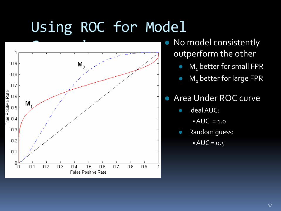
Using ROC for Model Comparison

47

No model consistently outperform the other

M1 better for small FPR

M2 better for large FPR

Area Under ROC curve Ideal AUC:

AUC = 1.0

Random guess:

AUC = 0.5

Cumulative Response Curve

Cumulative response curve more intuitive than ROC curve Plots TP rate (% of positives targeted) on the y-

axis vs. percentage of population targeted (x-axis)

Formed by ranking the classification “rules” from most to least accurate. Start with most accurate and plot point, add next

most accurate, etc.

Eventually include all rules and cover all examples

Common in marketing applications

48

Cumulative Response Curve

The chart below calls the one curve the “lift curve” but the name is a bit ambiguous (as we shall see on next slide)

49

Lift Chart

Generated by dividing the cumulative response curve by the baseline curve for each x-value.

Lift of 3 means that your prediction is 3X better than baseline (guessing)

Data Mining tools also generate non-cumulative curves that may be more insightful

50

Learning Curve

51

Learning curve shows how accuracy changes with varying sample size

Requires a sampling schedule for creating learning curve:

Arithmetic sampling (Langley, et al)

Geometric sampling (Provost et al)

Methods for Partitioning Data

Need to partition labelled data to form a training and test set (sometimes validation set)

Holdout Reserve fixed amount for training (2/3) and testing (1/3)

Random subsampling Repeated holdout

Cross validation Partition data into k disjoint subsets

k-fold: train on k-1 partitions, test on the remaining one

Leave-one-out: k=n

52

Cross-validation Partition data into k “folds” (randomly)

Run training/test evaluation k times

K=10 for 10-fold cross validation common

53

Cross Validation

Example: data set with 20 instances, 5-fold cross validation

training test

d1 d2 d3 d4

d5 d6 d7 d8

d9 d10 d11 d12

d13 d14 d15 d16

d17 d18 d19 d20

54

d1 d2 d3 d4

d5 d6 d7 d8

d9 d10 d11 d12

d13 d14 d15 d16

d17 d18 d19 d20

d1 d2 d3 d4

d5 d6 d7 d8

d9 d10 d11 d12

d13 d14 d15 d16

d17 d18 d19 d20

d1 d2 d3 d4

d5 d6 d7 d8

d9 d10 d11 d12

d13 d14 d15 d16

d17 d18 d19 d20

d1 d2 d3 d4

d5 d6 d7 d8

d9 d10 d11 d12

d13 d14 d15 d16

d17 d18 d19 d20

compute error rate for each fold then compute average error rate

Leave-one-out Cross Validation

Leave-one-out cross validation is simply k-fold cross validation with k set to n, the number of instances in the data set.

The test set only consists of a single instance, which will be classified either correctly or incorrectly.

Advantages: maximal use of training data, i.e., training on n−1 instances. The procedure is deterministic, no sampling involved.

Disadvantages: unfeasible for large data sets: large number of training runs required, high computational cost.

55

Multiple Comparisons

Beware the multiple comparisons problem The example in “Data Science for Business” is telling:

Create 1000 stock funds by randomly choosing stocks See how they do and liquidate all but the top 3 Now you can report that these top 3 funds perform very well (and

hence you might infer they will in the future). But the stocks were randomly picked!

If you generate large numbers of models then the ones that do really well may just be due to luck or statistical variations.

If you picked the top fund after this weeding out process and then evaluated it over the next year and reported that performance, that would be fair.

Note: stock funds actually use this trick. If a stock fund does poorly at the start it is likely to be terminated while good ones will not be.

56

cisc 4631 data mining - computer and information...

Documents