chromospheric line blanketing and the hydrogen …aa.springer.de/papers/7326001/2300287.pdf288 c.i....

Astron. Astrophys. 326, 287–299 (1997) ASTRONOMYAND

ASTROPHYSICS

Chromospheric line blanketing and the hydrogen spectrumin M dwarfsC.I. Short and J.G. Doyle

Armagh Observatory, College Hill, Armagh BT61 9DG, Northern Ireland ([email protected] – [email protected])

Received 13 December 1996 / Accepted 17 April 1997

Abstract. We present non-LTE calculations of the H i spectrumin a grid of chromospheric models that represents a dM0 star inwhich the activity level ranges from quiescent to very active. Weinvestigate three different treatments of the background opac-ity: 1) continuous opacity only, 2) blanketing due to lines thatform in the photosphere below Tmin, and 3) blanketing by linesthat form throughout the entire outer atmosphere. We show thatthe predicted Wλ of Lyα in all models is reduced by as muchas a factor of ≈ 4, and that of Hα in very active (dMe) starsis enhanced by a factor of about two by the inclusion of back-ground line opacity. A consistent treatment of line blanketingthat includes the effect of the chromospheric and transition re-gion temperature structure in the calculation of background lineopacity is necessary for the accurate calculation of Lyα, and insome cases Hα, in these stars. The Hα line in less active mod-els, and the Paβ line in all models, is negligibly affected by thetreatment of background opacity. We also show that, in addi-tion to the expected suppression of emergent flux in the visibleby line blanketing, the broad-band continuum flux in regionswhere λ < 2000A is increased by as much as a factor of threein some models by the inclusion of line blanketing. This reducesthe equivalent width of the Lyman series by a factor of four andis due to the veil of background lines going into emission inthe UV, and to the stronger coupling of the background sourcefunction to the Planck function in the presence of blanketingby thermal lines. We confirm the results of earlier calculationsthat suggest the dominance of the continuum emission in the ra-diative cooling of the chromosphere. Therefore, any proposedheating mechanisms must supply at least an order of magnitudemore non-radiative heating than would be required on the basisof an analysis in which only emission line cooling is considered.We also include a preliminary assessment of non-LTE effects inthe background opacity on the emergent UV continua.

Key words: stars: late-type – stars: activity – stars: chromo-spheres – line: formation

Send offprint requests to: C.I. Short

1. Introduction

Strong spectral lines play a special role in the modelling oflate-type stellar atmospheres because their cores are sensitiveto the outer layers where poorly understood non-radiative heat-ing processes affect the atmospheric structure (for a review, seeAvrett 1990). The spectrum of H i plays a particularly importantrole, not only because it contains strong lines, but because theionization balance of H i/H ii in the outer atmosphere partly de-termines the atmospheric structure. In a recent series of papers,Doyle et al. (1994), Houdebine & Doyle (1994), Houdebineet al. (1995), and Houdebine et al. (1996) have explored thedetailed line formation physics of the hydrogen spectrum in anextensive grid of chromospheric models of early M dwarfs. Thismonumental study includes an investigation of the response ofthe H i spectrum to atmospheric parameters and details of thechromospheric structure in models that span the entire range ofobserved activity level. This study provides a valuable guide tousing H i lines as semi-empirical chromospheric diagnostics.

Among the modelling achievements and important resultsof the above study are the following: 1) the construction of lowactivity models that can reproduce the very weak Hα absorp-tion of the ”zero Hα” dM(e) stars and simultaneously repro-duce the observed low surface flux of the Ca ii HK and Mg iihk emission lines in these stars (Doyle et al. 1994); 2) the de-termination of constraints on the mass loading, (mo), at theonset of the transition region at the top of the chromosphere(equivalent to determining the chromospheric pressure and thesteepness of the chromospheric gradient or the thickness of thechromosphere for a given value of Tmin), the temperature atthe onset of the transition region (8500 K in most cases), andthe thickness and functional form of the transition region thatis required to simultaneously fit the self-reversed Hα and Hβemission line profiles and the ratio of Lyα to Hα surface flux inthe most active (dMe) stars (Houdebine & Doyle 1994); 3) theconstruction of a comprehensive grid of chromospheric modelsthat successfully reproduces the observed morphology of theHα line in dM stars, from the lowest activity dM(e) stars to in-termediate activity stars with either strong Hα absorption or Hαemission wings and an absorption core, to the highest activitydMe stars with strong Hα emission. This grid has been used

288 C.I. Short & J.G. Doyle: Chromospheric line blanketing and the hydrogen spectrum in M dwarfs

to derive chromospheric diagnostics by comparing the relativeresponse of the various series of the H i spectrum (Lyman toBrackett) to changes in the structure of both the lower and upperchromosphere (Houdebine et al. 1995); and, 4) the modelling ofthe H emission continua and the hitherto unexpected realizationthat these continua, rather than the emission line spectrum, isthe dominant coolant in the chromospheres of those stars withrelatively hot Tmin values, and that the excess H i continuumemission in the highest activity stars decreases theU−B colourto an extent that is observable (Houdebine et al. 1996).

In the present investigation, we refine the above study by in-cluding additional physics: line blanketing of the radiation fieldin the non-LTE treatment of hydrogen. In general, the cores ofstrong lines that form at relatively low gas densities high in theatmosphere differ greatly from those predicted by calculationsdone with the approximation of Local Thermodynamic Equi-librium (LTE) (see the review by Avrett 1990). As a result, theline under investigation may depend on radiative rates in othertransitions of the atom, and these rates may be sensitive to thenon-local radiation field. Therefore, a detailed description ofthe background radiation field may be important for an accuratesolution of the non-LTE problem (see, for example, Mihalas(1978)). The reduction of non-LTE over-ionization in the UVcontinua of Fe i in the Sun due to the inclusion of line veilingin the background radiation field is a particularly instructiveexample (Rutten 1988).

Many previous non-LTE calculations of chromosphericlines have ignored line blanketing in the background radiationfield. Some have included photospheric line opacity only, as inthe case of the H i and Na i study in chromospheric dM starmodels by Andretta et al. (1997) (ADB henceforth), or the non-LTE multi-line chromospheric modelling of g Her (M6 III) byLuttermoser et al. (1994). Because the Lyman and Balmer lineseries and the Lyman continuum form well above Tmin, thestatistical equilibrium of hydrogen may be affected by blan-keting due to lines that form in the chromosphere (and tran-sition region in the case of Lyα) as well as blanketing due tophotospheric lines. Therefore, we have used the recently devel-oped PHOENIX model atmosphere code of Allard & Hauschildt(1995) to include line blanketing of the background radiationfield throughout the entire outer atmosphere, taking into accountthe chromospheric and transition region temperature structure.We discuss the behavior of chromospheric and transition regionline blanketing and assess its impact on the hydrogen equilib-rium and line formation physics in chromospheric models.

2. Computational method

2.1. Atmospheric models

Because the calculation of moderate resolution line opacity overa range of 50 000 A is computationally intensive, we considera restricted sample of six chromospheric models taken from thegrid presented by ADB. These models have as their photosphericbase a radiative equilibrium model calculated with PHOENIX(Allard & Hauschildt 1995). This photospheric model corre-

Fig. 1. Temperature structure of models in grid. 1A series: thin dashedline, 2A series: thick dashed line.

Table 1. Parameters of grid models

Series 1A Series 2Alog mo Tmin log mmin Tmin log mmin−6.0 2660 −2.72 2480 −3.72−4.8 2830 −1.70 2650 −2.70−3.8 2960 −0.80 2810 −1.80

sponds to a star of Teff = 3700 K, log g = 4.7, [AH ] = 0.0, andξT = 1.0 km s−1. These parameters correspond to a star of spec-tral type dM0 or dM1 (Lang 1992; Mihalas & Binney 1981).The PHOENIX model atmosphere code includes many impor-tant diatomic and triatomic molecules such as TiO and H2O inthe equation of state and opacity data and has been shown toprovide realistic models of early M stars (Allard & Hauschildt1995).

From each of the two model series of ADB labeled 1A and2A, we take models with the smallest, largest, and an interme-diate value of mo, which is the mass loading at the onset of thetransition region. These two model series differ in the value ofdT

dlogm in the chromosphere, with the series 2Amodels having a

steeper chromospheric temperature rise. Therefore, comparisonof spectral diagnostics computed with these two model series al-lows an assessment of the sensitivity to the location ofTmin andthe steepness of the chromospheric gradient (or, equivalently,the thickness of the chromosphere). The constancy of the chro-mospheric dT

dlogm in these models is in keeping with the results

of previous semi-empirical modeling of the outer atmospheresof a large variety of late-type stars (cf. Eriksson et al. 1983; Basriet al. 1981; Kelch et al. 1979 and other papers in those series).The value of dT

dlogm in the transition region, ( dT

dlogm )TR, is also

constant in these models, and we have chosen to use the sub-setof the grid that has a value of−6.5. The temperature at the top ofthe chromosphere where the transition region begins, T (mo), is

C.I. Short & J.G. Doyle: Chromospheric line blanketing and the hydrogen spectrum in M dwarfs 289

fixed at 8500 K following Houdebine & Doyle (1994). We onlyconsider models that are in radiative equilibrium below Tmin.Therefore, by fixing the value of Tmin, we also fix the value ofmmin, which is the mass loading at Tmin. Table 1 shows thechromospheric parameters of the grid models, and Fig. 1 showstheir temperature structure.

The increase in temperature throughout the chromospherehas an associated increase in the micro-turbulent velocity, ξT.In these models, ξT rises exponentially with decreasing log(m)in the chromosphere to a value of≈ 10 km s−1 atmo, then risesrapidly in the transition region to a value of ≈ 50 km s−1. Avalue of 10 km s−1 at the top of the chromosphere is typical ofvalues found for other late-type stars (see, for example, Erikssonet al. (1983) and papers in that series).

2.2. Line opacity

We have used PHOENIX to compute for our grid of models themean of the total mass absorption due to lines, κl, in 2A inter-vals from 500 to 25000A, and in 50A intervals from 25000 to50000A. The line lists used for the calculation incorporate thoseof Kurucz (1990), which contain about 58 million lines due toatoms and diatomic molecules, as well as the most recent andcomprehensive line lists for molecules of particular importancein M stars such as TiO and H2O. The total line list contains≈ 70 million lines. The PHOENIX code was originally devel-oped to compute atmospheric models of nova and supernova,therefore, it been proven over a wider range of temperature anddensity than most codes that are optimized for the atmosphericmodelling of M stars. Furthermore, PHOENIX calculates theline opacity by direct Opacity Sampling rather than by pre-tabulated Opacity Distribution Functions. Therefore, we wereable to computeκl at all depths from the base of the photosphereto a point in the lower transition region around a temperature of20 000 K.

The temperatures and densities in the upper chromosphereand lower transition region in our models correspond to the par-tial ionization of H i, which is, therefore, the main e− donorat those heights. The calculation of the ionization equilibriumof H i in the chromosphere is complicated by severe non-LTEeffects. Therefore, the Ne structure used in the calculation ofκl is calculated from a multi-level non-LTE solution of the cou-pled radiative transfer and statistical equilibrium equations forthe first five levels of H i using an operator splitting/acceleratedlambda iteration procedure that is incorporated into PHOENIX.The Ne structure and the value of κl in the chromosphere mayalso be affected by the non-LTE ionization of various met-als. Therefore, we have also treated in non-LTE some of thosespecies for which PHOENIX incorporates detailed atomic mod-els: the first five levels of Mg ii and Ca ii, the first ten levels ofHe i and He ii, and the first three levels of Na i.

2.3. Non-LTE hydrogen

We have used the code MULTI (Carlsson 1986) to solve thecombined radiative transfer and statistical equilibrium equations

for an atomic model that incorporates the lowest nine levels ofH i and the H ii state. Because the chromospheric Ne densitystructure is determined by the H i/H ii ionization balance, weiterate the non-LTE solution and the equation of hydrostaticequilibrium to convergence. The radiative transfer problem issolved in detail for all 36 b− b transitions connecting the nineH i states and for the b − f transitions of these states. The cal-culation of the background radiation field includes the additionof the PHOENIX line opacities, κl, to the continuous opacitynormally computed by MULTI. These were incorporated usinga modified version of MULTI that was presented in ADB. Forthe b− b transitions, κl was included in the Lyα, Hα, and Paβlines as a straight arithmetic mean in 2A intervals. We includedblanketing in the first two of these because of their importantrole in the statistical equilibrium of H i, and in the latter be-cause we wish to develop the detailed line shape of Paβ as achromospheric diagnostic (Paα is generally too contaminatedby telluric absorption to be a useful). For the b−f transitions, κlwas included as a harmonic mean in 100A intervals. An intervalwidth of 100A is necessary because normally a sparse frequencysampling of the b − f continua is used in MULTI calculationsin order to control the computation time. A harmonic mean wasused because occasional strong lines have a disproportionatelylarge effect on the straight mean in a large wavelength interval.

ADB also included background line opacities computedwith PHOENIX in their non-LTE H i/ii calculation with thesame models. However, they were able to compute κl for aphotospheric model only. For their chromospheric models theygradually ramped the value of κl down to zero, ad hoc, over adecade in column mass density aboveTmin. In order to compareour results with previous studies, we have used our procedureto calculate κl for a radiative equilibrium model and rampedit down to zero just above Tmin using the same procedure asADB. We then re-calculated the non-LTE H i/ii andNe solutionusing these photospheric κl tables. For clarity, we henceforthdesignate as κc

l the line opacity that reflects the chromospheric

and transition region temperature structure, and as κpl the line

opacity that is purely photospheric.

3. Results and discussion

3.1. Chromospheric line blanketing

Figs. 2 and 3 show the ratio ofκcl to the total continuous mass ab-

sorption,κc, in the 500 to 12000A range for the lowest and high-est pressure models in the 1A series, respectively. The dashed

lines indicate the location of Tmin. The value ofκclκc

reaches alocal minimum near Tmin, then begins to rise again with de-creasing m in the lower chromosphere. This mirrors the rise ofκl with increasingm in the upper photosphere just below Tmin.In the upper chromosphere the higher temperatures dissociatemolecules and ionize many metals leading to a decrease in κc

lin this wavelength regime, and finally an abrupt decline in thetransition region. The initial rise in κc

l above Tmin differs fromthe ad hoc gradual ramping down of κl above Tmin in the cal-


Fig. 2. Ratio of line to continuous absorption opacity,κcl

κc, computed

by PHOENIX for the lowest pressure model in 1A series. The dashedlines show the position of Tmin.

Fig. 3. Same as Fig. 2 for the highest pressure model in 1A series.

culations of ADB. Therefore, their treatment of transitions thatform in the upper chromosphere and transition region are basedon background opacities that are significantly under-estimated.

3.2. Radiative transfer in hydrogen

Fig. 4 shows the emergent flux, Fν(τ = 0), in the Lyman andBalmer continua as computed by MULTI for the lowest andhighest pressure models in the 1A series, with κc only, withκ

pl , and with κc

l . The Lyman jump is strongly in emission inthe highest pressure model. The H i lines have been left out ofκl because they are treated in detail in the MULTI calculation.All the important b-f continua of metals that are treated by the

Fig. 4. The Fν (τ = 0) distribution for the radiative equilibrium model(thick lines), and chromospheric models of lowest (top panel) and high-est (bottom panel) pressure in the 1A series. Solid line:κc only; dashedline: κc

l ; dotted line: κpl .

Uppsala Opacity package that accompanies MULTI have beenincluded in all calculations. However, the presence of κl ob-scures the corresponding jumps in the Fν(τ = 0) distribution.In the region just to the blue of the Balmer jump, the inclusionof κc

l lowers Fν(τ = 0), which is consistent with the expectedbehavior of a blanketed radiation field. However, at still shorterwavelengths in the Balmer continuum, κc

l has the opposite ef-fect and causes Fν(τ = 0) to be larger. For the lowest pressuremodel, this behavior extends to the blue side of the Lyman jump,where Fν(τ = 0) is larger by ≈ 0.5 dex in the case of κc

l . The

main qualitative differences between the cases of κcl and κ

pl are

that the κpl predicts largerFν(τ = 0) in the 1500 to 2500A range

of the Balmer continuum, and lower Fν(τ = 0) in the Lymancontinuum, compared to κc

l values.Fig. 5 shows the mean intensity, Jν , the monochromatic

background intensity source function,Sν , and the intensity con-tribution function,CI, for an angle near disk center (µ = 0.887),at two wavelengths on the Balmer continuum, for the cases ofκc only, and κc

l values. The Planck function,Bν , is also shown.For λ <∼ 3647A, in both models, the inclusion of κl causes Jνto be reduced throughout most of the atmosphere, as expected.However, the effect of κc

l on Fν(τ = 0) is controlled by thecondition that Sν ≈ Bν at the depths where CI is maximal, andthe inclusion of κc

l causes the peak of CI to move outwards.

Because CI peaks well below Tmin, the inclusion of κcl causes

Fν(τ = 0) to form at depths where Bν is lower, and, hence,Fν(τ = 0) is reduced.

Further along the Balmer continuum, at λ = 1600A, thedepth distribution ofCI is weighted more toward chromosphericdepths, where Sν <∼ Bν . The inclusion of κc

l raises the chro-


Fig. 5. Various radiative transfer quantities for λ = 3647A (top panels)and λ = 1600A (lower panels) for the lowest (left panels) and highest(right panels) pressure models in the 1A series. The thin solid line,thick solid line, and thin dotted line are Jν , CI, and Sν , respectively,for µ = 0.887, for the case of κc only. The thin short-dashed line, thickshort-dashed line, and thick dotted line are the same quantities for thecase of κc

l . The long-dashed line is Bν .

mospheric part of CI and shifts CI to shallower depths aboveTmin where Bν , and hence Sν , is larger. Furthermore, the in-clusion of κc

l raises Sν in the upper chromosphere. Both ofthese effects cause Fν(τ = 0) to be increased. The increase inSν in the upper chromosphere in the case of κc

l is partly dueto a very small increase in Jν at these depths. Normally oneexpects line blanketing to decrease the value of Jν . However,κc

l will generally include many lines that form at depths aboveTmin, and that have line source functions that are dominatedby the thermal contribution (Sl <∼ Bν). At λ < 3650A andT ≈ 6000 K, Bν is very sensitive to temperature, and at thechromospheric depths where these lines form, we may have thecondition: Jl ≈ Bν > Jcontinuum. In other words, the chro-mospheric temperature inversion may drive many of these linesin to net emission, and κc

l may become a net contributor to Jν inthe UV. This is consistent with the greater size of the Jν increasein the highest pressure model. The resulting increase in Jν isslight and can only account for a small fraction of the increase inSν . The rest of the increase in Sν in the case of line blanketingis the result of κl being treated as a purely thermal source ofopacity which, therefore, increases the relative contribution ofBν to the value of Sν .

Fig. 6 shows the same quantities as Fig. 5, but for λ = 911A.The situation differs from that of the Balmer continuum in thatCI is sharply peaked at depths in the uppermost chromosphereand transition region. Because of the much larger value of thecontinuous opacity in the Lyman continuum, Sν = Bν through-out almost the entire atmosphere. However, in the lowest pres-sure model,Sν <∼ Bν in the uppermost part of the chromosphere

Fig. 6. Same as Fig. 5, but for λ = 911A. The lower panels showthe same quantities as the upper panels, but on an expanded scale incolumn mass density.

whereCI is maximal. This slight departure from LTE allows thevalue of Jν to influence Sν , and furthermore, this figure showsthat Jν in the upper chromosphere is increased slightly by theinclusion of κc

l , as was the case at λ = 1600A. Therefore, Sν ,

and consequently Fν(τ = 0), are increased by κcl . For the high-

est pressure model, Sν = Bν throughout the entire atmosphere,and CI is so sharply peaked in the narrow transition region,that the inclusion of κc

l does not affect its location or value.

Therefore, κcl has negligible effect on Fν(τ = 0).

3.3. The NH i and Ne density structure

The left panel of Fig. 7 shows the radiative rate per atom fromthe n = 1 and n = 2 states of H i throughout the chromospherein the same two models. Because the hydrostatic equilibriumpopulation of H i and the statistical equilibrium population ofthe level populations may both be different for the cases with andwithout line blanketing, we show in the right panel the radiativerate per volume element. Figs. 5 and 6 show that for the lowestpressure model, in the case where κc

l is included, Jν at 911 and3647A is lower throughout the Tmin region and most of thechromosphere. Correspondingly, the radiative ionization ratesfrom n = 1 and n = 2 are lower throughout the chromosphere.

Fig. 8 shows the NH i and NH ii population densities nor-malized by the total H population density of the lowest andhighest pressure models in the 1A series for the cases κc andκc

l . Fig. 9 show the corresponding Ne population density and

also includes the case of κpl . The effect of including κc

l is mostpronounced in the lowest pressure model where it reducesNe byas much as≈ 0.3 dex at some depths in the chromosphere. Theeffect of κc

l is less pronounced in the highest pressure model.As expected, the decrease in Ne in the chromosphere caused


Fig. 7. Radiative ionization rates for H i from the n = 1 (thin lines) andn = 2 (thick lines) states for the lowest (top panel) and highest (bottompanel) pressure models in the 1A series. Solid line: κc only; dashedline: κc

l . Left panel: rates per atom; right panel: rates per unit volume.

by κcl is mirrored by a corresponding decrease in NH ii. How-

ever, the effect on the H i/H ii balance due to κcl persists deeper

into the atmosphere by over two decades in column mass densitythan the effect onNe. Unlike solar type stars, hydrogen remainsmostly neutral until near the top of the chromosphere, as can beseen from Fig. 8. Therefore, the details of the H i/H ii balanceonly have a significant effect on the Ne density in the upperchromosphere. As a corollary, we conclude that it is necessaryto determine the effect of κc

l on the ionization equilibria of met-als that are important electron donors in the lower chromosphereand Tmin region, as well as on the H i/H ii balance, in order toproperly assess the sensitivity of the Ne density throughout theentire chromosphere to the opacity treatment.

The dotted line shows theNe density resulting from a calcu-lation with κ

pl . The neglect of the chromospheric component of

the line blanketing causes Ne to be underestimated by ≈ 0.05dex near the top of the chromosphere in the lowest pressuremodel. In the highest pressure model, the two treatments of κlproduce Ne densities that differ negligibly.

Any differences in the final NH i and Ne density that resultfrom different treatments of the opacity may have two sources:1) the H i/H ii balance will differ as a result of different amountsof total opacity being included in the calculation of the radiativerates of the hydrogen transitions, 2) because the hydrostaticequilibrium equation was re-converged separately for each case,the equilibrium density structure differs for each case. In orderto determine the relative importance of these two effects, wealso show in Fig. 9 the Ne density normalized by the total Hpopulation (Ne/(H i + H ii)). Noting that the y− axis scale isnecessarily more compressed in the Ne/NH plot, Fig. 9 showsthat the differences in Ne between the cases with and without

Fig. 8. The NH I/NH total (thick lines) and NH II/NH totalnumber density (thin lines) resulting from non-LTE H i solution forthe lowest (top panel) and highest (bottom panel) pressure models inthe 1A series. Dotted line: κc only; dashed line: κc

l .

κcl are almost entirely due to direct radiative transfer effects

on the H i/H ii balance. The reduction in Ne and NH II valuesdue to κc

l are consistent with the reduction in radiative photo-ionization rate seen in Fig. 7 and this is consistent with thechanges being directly due to radiative transfer effects. For thehighest pressure model, the effect of κc

l on both the Jν valuesand the radiative rates is rather smaller, which corresponds tothe smaller effect on the Ne and NH II densities.

3.4. The hydrogen spectrum

3.4.1. Lyα

Fig. 10 shows the Lyα flux profile for our entire grid with κconly and with κc

l . Also shown are line profiles for the 1A series

with κpl . The computed flux level of the emission peaks and the

central reversal for all the models is negligibly affected by theinclusion of κl and by the particular treatment of κl. Therefore,the absolute brightness of the line near ∆λ = 0 may be usedas an accurate chromospheric and transition region diagnosticwithout the inclusion of κl. However, the inclusion of κc

l causesthe computed flux level of the continuum in the region of Lyα tobe increased by as much as≈ 0.3 dex. This increase is consistentwith the behavior of the computed broad-band continuum shownin Fig. 4.

The increase in the local continuum level is reduced to thepoint of being negligible in the case of κ

pl . The effect of includ-

ing κl in the photosphere, but neglecting it in the chromosphere,can be understood from a consideration of Figs. 5 and 6. For λin the range 912 to 1600A, CI arises largely at chromospheric

depths. Therefore, κpl neglects line blanketing in the part of the


Fig. 9. TheNe (left panel) andNe/NH (right panel) population densityresulting from the non-LTE H i solution for the lowest (top panel) andhighest (bottom panel) pressure models in the 1A series. Solid line: κconly; dashed line: κc

l , dotted line: κpl .

Table 2. Wλ of Lyα

log mo Wλ in A

1A Series κc κpl κc

l−6.0 −2.14e + 03 −2.04e + 03 −8.57e + 02−4.8 −1.85e + 04 −1.86e + 04 −4.30e + 03−3.8 −1.36e + 04 −1.50e + 04 −3.71e + 03

atmosphere where the background Fν(τ = 0) at λ = 1215A isforming. Therefore, if the relative brightness of the line corewith respect to the local continuum, or the equivalent width,Wλ, is to be used as a diagnostic, then the accuracy will beaffected by the treatment of background opacity. Table 2 givesthe Wλ values for the models of the 1A series with the variousopacity treatments. The value of Wλ is reduced by as much as75% by κc

l in the case of the highest pressure model. This largechange in Wλ is difficult to see by visual inspection of Fig. 10.However, a ≈ 0.3 dex increase in the background Fν(τ = 0)corresponds to about a factor of five increase in linear flux units.Because the Fν(τ = 0) level of the line core does not changesignificantly when κc

l is added, the total area of the emissionabove continuum decreases by an amount that is approximatelyproportional to the increase in background Fν(τ = 0).

3.4.2. Hα

Fig. 11 shows the computed Hα profiles for the entire grid withκc only, and with κc

l . Also shown are line profiles for the 1A

series only with κpl . Table 3 shows theWλ values for the models

in the 1A series with the various opacity treatments. Compari-

Fig. 10. Lyα flux profiles. Left panel: κcl ; right panel: κc only. Models

in series 1A: thin dashed line; 2A series: thick dashed line; the 1A seriesonly with κ

pl : dotted line. The lowest and highest pressure models are

the ones that have the weakest and strongest line emission, respectively.

Fig. 11. Hα flux profiles. Left panel: κcl ; right panel: κc only. Models

in series 1A: thin dashed line; 2A series: thick dashed line; the 1Aseries with κ

pl : dotted line. The lowest pressure models are the ones

that have the weakest line absorption.

son of the left and right panels of Fig. 11 shows that inclusionof κl causes the ”continuum” to be noticeably depressed anddistorted. It is not straight-forward to rectify the computed lineprofiles to a continuum level of unity because the backgroundradiation is not a true continuum due to the inclusion of lineblanketing. Therefore, we have plotted absolute flux and thecomparison of line profiles between the calculations with andwithout κl is with respect to their respective continua.

Historically, the morphology of Hα has been the main di-agnostic for classifying dM stars by activity level, and Fig. 11


Table 3. Wλ of Hα

log mo Wλ in A


l−6.0 0.075 0.050 0.055−4.8 0.710 0.680 0.705−3.8 −3.560 −7.124 −6.375

Table 4. Integrated line flux in Lyα and Hα and Lyα/Hα in dMe (logmo = −3.8) models

Models κc κpl κc

lLyα flux (ergs s−1 cm−2 A−1)

1A Series 1.57e + 07 1.58e + 07 1.57e + 072A Series 1.64e + 07 1.65e + 07 1.65e + 07

Hα flux (ergs s−1 cm−2 A−1)1A Series 3.77e + 06 4.41e + 06 4.32e + 062A Series 3.74e + 06 4.34e + 06 4.28e + 06

Lyα/Hα1A Series 4.16 3.57 3.642A Series 4.40 3.81 3.87

shows that our grid spans the range of observed activity levelfrom the least active dM(e) stars (profile with almost no ab-sorption) to very active dMe stars (profile with the strongestemission). For the highest pressure model, the flux level of theemission peaks and central reversal are negligibly affected byκc

l , but the Wλ value of the net emission above continuum isapproximately doubled due to the depression of the continuum.For the models where the profile is in absorption, the effect onWλ is negligible. Therefore, Hα modelling of dMe stars in par-ticular must incorporate κc

l in order to be accurate. The profilesof all the models are negligibly affected by the choice betweenκc

l and κpl .

The Lyα to Hα flux ratio in dMe stars is a diagnostic of thethickness of the transition region (Houdebine & Doyle 1994).Table 4 shows the integrated line fluxes and the flux ratio in ourmost active models with the different treatments of line blanket-ing. The large dependence of Wλ on background opacity treat-ment shown in Tables 2 and 3 is proportional to a correspondingchange in the background continuum level. Therefore, the totalflux in the emission lines has a much weaker dependence. How-ever, the Lyα to Hα flux ratio is reduced by≈ 12 to 15% in thecase of line blanketing. The flux ratio is only marginally affectedby the choice between κ

pl and κc

l . From Fig. 14 of Houdebine& Doyle (1994), we estimate that the neglect of line blanketingwould cause an estimate of the transition region thickness basedon a fit to Lyα/Hα flux to be too small by a factor of<∼ 2. Doyleet al. (1997) present observed values of FLyα/HLyα that havebeen corrected for the interstellar attenuation of Lyα for a va-riety of M drawfs. For Gl278C (dM1.0e), they find a value of3.5, which is in excellent agreement with value calculated herewith line blanketing included.

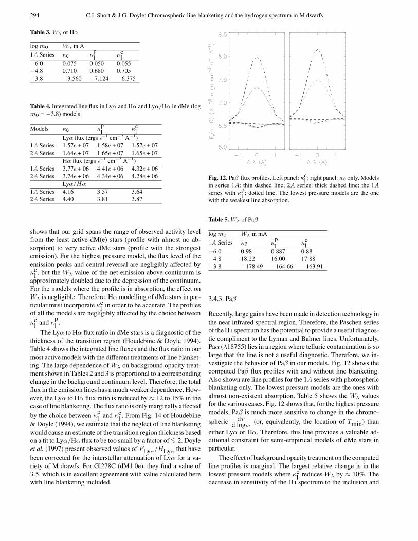
Fig. 12. Paβ flux profiles. Left panel: κcl ; right panel: κc only. Models

in series 1A: thin dashed line; 2A series: thick dashed line; the 1Aseries with κ

pl : dotted line. The lowest pressure models are the one

with the weakest line absorption.

Table 5. Wλ of Paβ

log mo Wλ in mA


l−6.0 0.98 0.887 0.88−4.8 18.22 16.00 17.88−3.8 −178.49 −164.66 −163.91

3.4.3. Paβ

Recently, large gains have been made in detection technology inthe near infrared spectral region. Therefore, the Paschen seriesof the H i spectrum has the potential to provide a useful diagnos-tic compliment to the Lyman and Balmer lines. Unfortunately,Paα (λ18755) lies in a region where telluric contamination is solarge that the line is not a useful diagnostic. Therefore, we in-vestigate the behavior of Paβ in our models. Fig. 12 shows thecomputed Paβ flux profiles with and without line blanketing.Also shown are line profiles for the 1A series with photosphericblanketing only. The lowest pressure models are the ones withalmost non-existent absorption. Table 5 shows the Wλ valuesfor the various cases. Fig. 12 shows that, for the highest pressuremodels, Paβ is much more sensitive to change in the chromo-

spheric dTd logm (or, equivalently, the location of Tmin) than

either Lyα or Hα. Therefore, this line provides a valuable ad-ditional constraint for semi-empirical models of dMe stars inparticular.

The effect of background opacity treatment on the computedline profiles is marginal. The largest relative change is in thelowest pressure models where κc

l reduces Wλ by ≈ 10%. Thedecrease in sensitivity of the H i spectrum to the inclusion and


Table 6. Relative contribution to radiative cooling

Unblanketed Blanketedlog mo Lines Continuum Lines Continuum

Series 1A−6.0 0.000 0.000 0.000 0.000−4.8 0.017 0.983 0.013 0.987−3.8 0.174 0.826 0.114 0.886

Series 2A−6.0 0.001 0.999 0.006 0.994−4.8 0.015 0.985 0.014 0.986−3.8 0.190 0.810 0.164 0.836

treatment of κl as λ increases is consistent with the generaldecrease in spectral line blanketing as λ increases.

3.5. Chromospheric energy budget

One of the important conclusions of Houdebine et al. (1996)is that, contrary to what has been assumed previously, chromo-spheric radiative cooling in the emission continuum is greaterthan that in the H i emission lines for many chromospheric mod-els. For their series of models with the largest value of Tmin(3000K), they find that the relative contribution of the total H iseries to the energy loss is at most 15%. For their lower Tmin(2660K) models, the continuum contribution is about 50%. Forboth the lines and continuum, they define cooling as the excessflux above that from a basal flux model with minimal emission.The model with the lowest total emission (continuum + H i lines)in our grid is the lowest pressure model of the 1A series. Wetake this model as a fiducial basal flux star and subtract its H iline spectrum and continuum emission from each of the othermodels in the grid to produce excess emission values.

Table 6 shows the relative contribution to the total excess ofthe total H i line series up to and including the series of nl = 5,and of the total H i continuum emission up to and including theB-F continuum of the n = 5 level. We confirm, qualitatively, theresult of Houdebine et al. (1996) for the higher Tmin models,where we find that the continuum carries over 80% of the ex-cess flux at high chromospheric pressure. We also confirm thetrend shown in their Fig. 7 toward increasing dominance of thecontinuum as chromospheric pressure decreases. However, ourresults differ radically from those of Houdebine et al. (1996)for lower Tmin models, where we find that the continuum isdominant as in the higher Tmin models. Lines play a minor rolein the chromospheric energy loss throughout our entire grid. Atthis time we are unsure of the reason for the difference in theresults for the lower Tmin models. Fig 13 shows the overall dis-tribution ofFν(τ = 0) for the entire grid. The strong response ofthe blue and UV continuum to increasing chromospheric pres-sure, combined with the large wavelength range over which theexcess flux contributes, accounts for the dominant role of thecontinuum in the energy balance. Table 6 shows that the inclu-sion of κc

l has a minor effect on the relative contributions, andshifts the balance even more toward the continuum.

Fig. 13. Overall Fν (τ = 0) distribution for entire grid. Upper panel:κc

l ; lower panel: κc only. Models in series 1A: thin dashed line; 2Aseries: thick dashed line; radiative equilibrium model: solid line.

These results are only approximate because the emergentflux in a transition is only equal to the total cooling in thattransition if the transition is optically thin. The central dou-ble reversal of the Lyα and Hα line profiles indicate that thereis some chromospheric self-absorption in these transitions andthat, therefore, τ > 1 at ∆λ ≈ 0. Therefore the cooling ratefor a particular transition computed here and in Houdebine etal (1996), especially in the case of a line, is only a lower limit.Nevertheless, the dominance of the continuum in the total loss isso large that it is unlikely to be entirely due to an underestimatein the line cooling.

The amount of non-radiative heating required to energize thechromospheres of late-type stars is a fundamentally importantconstraint on theoretical heating mechanisms. Traditionally, theamount of heating has been measured by summing the excessflux in emission lines such as the H i Lyman and Balmer seriesand the Ca ii and Mg ii resonance doublets. However, the resultsshown here indicate that the energy loss in these lines may beonly a small fraction of the excess flux in the continuum, and,therefore, the total cooling rates are much larger than previouslythought.

3.6. Background non-LTE effects

3.6.1. Metallic b− f continua

There are at least two important limitations in the computationof the emergent UV flux in both this work and in that of Houde-bine et al. (1996). The first is that the background continuousabsorbers have been treated in LTE. In their detailed modellingof the solar atmosphere, Vernazza et al. (1981) (VAL) showedthat the continuum between 1000 and 1200 A is reduced byabout an order of magnitude as a result, largely, of the ground


state C i b−f continuum being out of LTE. VAL tabulate depar-ture co-efficients, bi, for the first eight levels of C i, Si i, Mg i,and Al i, and for eight combined levels of Fe i, all of whichshowed large non-LTE departures in their model. The lower ex-citation energy levels that are more heavily populated have bi

values that fall as low as≈ 0.1 in the Tmin region where the nearUV continuum forms, and then rise to values of ≈ 100 in theupper chromosphere. To properly account for non-LTE metallicopacity in our models, we should solve the combined radiativetransfer and statistical equilibrium equations for at least thesefive elements, then re-compute the non-LTE H i/ii solution andhydrostatic equilibrium equation with the modified backgroundopacity and metallic ne contribution, and iterate this procedureuntil the ne values converge at all depths. This is a massive com-putational undertaking and is beyond the scope of the currentstudy. However, we intend to perform such a calculation oncewe have acquired all the necessary atomic data.

For now, we have made an initial estimate of the importanceof metallic non-LTE departures with respect to the Sun in de-termining Fν(0) in the UV by scaling the chromosphere andphotosphere of the VAL solar model to one of our models (thelowest pressure model in the 1A series), and interpolating theVAL bi values for the five metals listed above onto our model.We then recomputed Fν(0) with the VAL bi values incorporatedinto the calculation of the background opacity. There are at leasttwo sources of error in this procedure: 1) The VAL bi values aredetermined by the particular densities and radiative intensitiesin the VAL model; a full non-LTE treatment of the metals in ourmodel will certainly yield different bi values, and 2) we are onlytaking into account the non-LTE departures of the level popula-tions; the b− f source function, Sν , is still equal to the Planckfunction in our calculation. Therefore, this is not a consistentnon-LTE treatment of the background continuous opacity. Nev-ertheless, it gives us an approximate indication of the extent towhich Fν(0) is sensitive to the metallic bi values as comparedto the solar case.

The left panels in Fig. 14 show Fν(0) with κc in LTE andwith the VAL bi values. The upper panel shows the importantUV region and the lower panel shows the overall distribution.The left and right panels show the cases where κl blanketing isexcluded and included, respectively. Careful examination of theupper panel shows that the 1000 to 1200 A region (logλ = 3.0to 3.1 in the figure) is more affected by the metallic bi valuesthan the nearby regions, with the flux there being suppressedby non-LTE effects. This is in general agreement with the VALresults for the Sun, however, the effect is much less that the orderof magnitude Fν(0) reduction found for the VAL solar model.For both the VAL model and our dM star model, κc throughoutmost of the photosphere and lower chromosphere is dominatedby C I around λ1000 A and by C I and Si i around λ1200 A,and in both cases the effect of non-LTE departures is to enhancethe contribution of both metals so that they provide ≈ 100%of the opacity. The difference in the behavior of Fν(0) betweenthe two models when departures are allowed for must dependon the exact location of the continuum formation in this regionin each model. Due to the crudeness of our non-LTE treatment

Fig. 14. The effect of various opacity treatments on Fν (0). Left panels:κc only - LTE treatment (solid line), VAL bi values for five metals(dotted line). Right panels:κc

l blanketing -κc in LTE (solid line),κc withVAL bi values (dotted line), κc in LTE and a line scattering albedo in κl

for the case of minimal scattering (long dashed line) and Anderson’satomic scattering (short dashed line). Top panels: UV region. Bottompanels: overall distribution.

in the M star model, further analysis of the difference in Fν(0)behavior between the two models is unwarranted at this time.Inspection of the right panel shows that the Fν(0) suppressiondue to non-LTE b− f effects is reduced to negligibility by theinclusion of line opacity.

Also, we find an enhancement in Fν(0) due to non-LTEdepartures in the logλ = 3.15 to 3.2 region. At λ = 1500A thedominant contributor changes from Si i to a combination of Si i,Mg i, and Al i as λ increases. These metals contribute close to100% of the opacity in both the LTE and non-LTE case. Onceagain, an explanation of the excess Fν(0) in the non-LTE casewill require a careful study of where the continuum forms andshould wait until the non-LTE treatment of metals in our modelis treated properly.

We conclude tentatively that the impact of metallic non-LTEdepartures on the UV emission in our models is significantly lessthat found for the Sun by VAL and probably does not effect ourconclusion that the continuum emission dominates the chromo-spheric energy budget. However, a self-consistent solution ofthe non-LTE problem for hydrogen and all five dominant met-als must be undertaken for our models before we can reach adefinite conclusion on this point.

3.6.2. Background line scattering

The second limitation in this work is that the line blanketingopacity, κl, is assumed to be entirely thermal throughout themodel. The extensive non-LTE line blanketing calculation ofAnderson (1989) for the Sun demonstrates that many atomic


Fig. 15. Top panel: approximate line thermalization parameter, ε at -926 A (dotted line), 1026 A (dashed line), 1226 A (squares), 3836 A(solid line), 4863 A (thick dashed line). Bottom panels: line scatteringalbedo, σ. Anderson’s albedo parameter, q, equal to 6.0 × 1012 (leftpanels), and 1.0× 109 (right panels).

and ionic lines become scatterers rather than thermal absorbersof radiation in the upper photosphere of a radiative equilibriummodel where the gas density becomes relatively low. As a result,our thermal treatment has the effect of keeping Sν artificiallyclose in value toBν in the outer layers where the UV continuumis forming. In the case of coherent isotropic scattering the linesource function, Sl, is approximately given by

S = J+εB1+ε , (1)

and the extent to which a line is scattering rather than absorbingis determined by the relative weights of J andB in this sum. Theline thermalization parameter, ε, is equal toCij/Aij, whereCij isthe rate of collisional transitions between the upper and lowerstates, andAij is the rate of spontaneous radiative decay from theupper state. The dependence on Cij makes ε depth dependent,and Anderson (1989) has suggested the following approximateformula for ε:

ε = Neq(hν)3 , (2)

where hν is in eV and q = 6×1012 for Fe i lines and 7×1013 forionic lines. Furthermore, the line scattering albedo, σ, is equalto 1/(1 + ε).

We have modified our treatment of κl by adding the quantityσ×κl to the total scattering opacity and (1−σ)×κl to the totalthermal opacity at each depth. The purely thermal treatment ofκl that was described in the previous sections corresponds tothe case of σ = 0. Our κl tables include all lines from atoms,ions, and molecules added together. Therefore, we are not able totreat lines from different types of absorbers separately. However,we have tried two extreme values of q found in the literature:

Table 7. Relative flux excess in UBV with respect to basal model(series 1A, log mo = −6.0)

Unblanketed Blanketedlog mo U B V U B V

Series 1A−6.0 0.000 0.000 0.000 0.000 0.000 0.000−4.8 0.012 0.010 0.008 0.030 0.023 0.026−3.8 0.039 0.023 0.018 0.151 0.049 0.078

Series 2A−6.0 0.007 0.005 0.004 0.030 0.008 −0.002−4.8 0.017 0.014 0.011 0.027 0.023 0.025−3.8 0.038 0.022 0.017 0.275 0.091 0.043

Anderson’s atomic value of 6 × 1012, and a value of 1.0 ×109 that that corresponds to mostly thermal lines with minimalscattering (Avrett et al. 1994). The right panels of Fig. 14 showthe computed Fν(0) with σ included in the treatment of κl. Fig.15 shows the value of ε and σ throughout the model for bothvalues of q.

For q = 6 × 1012, ε, as computed by the approximate for-mula, is very low (< 10−4) throughout most of the model abovethe deep photosphere. As a result, σ is almost unity and Fν(0)for logλ > 3.3 is an order of magnitude brighter than that ofthe thermal case and is indistinguishable from that of an un-blanketed model because the lines are barely absorbent. How-ever, for logλ < 3.3, Fν(0) is reduced by ≈ 0.2 dex with re-spect to the thermal case. Hoflich (1995) has suggested that thevalue of ε based on the treatment of Anderson (1989) may be asmuch as two orders of magnitude too small, which may accountfor the underblanketing found with the atomic q parameter atlogλ > 3.3. At the other extreme, q = 1 × 109 gives an Fν(0)distribution that differs negligibly from the purely thermalFν(0)for logλ > 3.3. For logλ < 3.3,Fν(0), is very close to that com-puted with the much higher q value. This relative insensitivityof the mid-UV flux to the albedo is due to the rapid increase ofσ with decreasing Ne and decreasing λ, which causes σ to be≈ 1 at the depths where radiation with λ < 3.3 forms for bothvalues of q.

The 0.2 dex decrease in the UV flux due to line scatteringwith either extremal value of q is much less than the four ordersof magnitude difference between the UV Fν(0) values for thechromospheric model and the radiative equilibrium model. Weconclude, for now, that the chromosphere produces substantialexcess continuum emission, even in the presence of blanketingby scattering lines.

The extent to which the non-LTE departures discussed aboveaffectFν(0) may depend on the chromospheric pressure. There-fore, these effects will be investigated, more accurately, for theentire grid of models in a future study.

3.7. Photometric colours

Houdebine et al. (1996) have found that in the highest pressurechromospheric models, the structure of the outer atmosphere has


Table 8. Computed colours of grid models

Unblanketed Blanketedlog mo TR U −B B − V U −B B − V

Series 1A−6.0 0.286 1.031 1.481 1.123−4.8 0.284 1.029 1.473 1.126−3.8 0.269 1.027 1.381 1.151

Series 2A−6.0 0.285 1.030 1.458 1.111−4.8 0.283 1.028 1.477 1.124−3.8 0.270 1.026 1.312 1.073

a detectable effect on the U − B colour due to the increasingenhancement of Fν(τ = 0) with decreasing λ seen in Fig. 13.In Table 7, we show for our grid of models with and withoutline blanketing the excess flux with respect to the basal modelnormalized by the flux from the basal model in the JohnsonUBV pass-bands. In Table 8, we show the computedU−B andB−V colours. For the unblanketed models, the highest pressuremodel has a value ofU−B that is 0.015 magnitudes lower thanthat of the lowest pressure model. The changes in Fν(τ = 0)due to the addition of κc

l increase U −B by ≈ 1.1 magnitudesand B − V by ≈ 0.3 magnitudes. The sensitivity of U − B tochromospheric pressure is reduced somewhat in the presenceof κl, but is still significant; the difference between the lowestand highest pressure models is reduced to ≈ 0.01 magnitudes.Therefore, we confirm the result of Houdebine et al. (1996) thatthe chromospheres of the most active stars should be detectablewith centimagnitude precision broad band photometry in theviolet and blue spectral regions.

Amado & Byrne (1997) have analysed de-reddened two-colour diagrams in the Johnson system for a large sample (n >100) of late-type stars with B−V in the range 0.2 to 2.2. Theyhave found that stars classified as ”active” on the basis of theirobserved Hα profile, on average, have a U − B colour that is0.042 magnitudes bluer, with σ = 0.0872, than inactive stars.They caution that the dependence of colour on metallicity hasnot been accounted for in their study. However, their resultssuggest that there is a U − B dependence on chromosphericactivity at the centimagnitude level found in our calculations.

4. Conclusion

The predicted Wλ of the Lyα emission line is strongly reduced,and that of the Hα emission line in active (dMe) stars is stronglyenhanced by the inclusion of line blanketing in the backgroundopacity in the non-LTE hydrogen calculation. In less active starsonly Lyα is significantly affected. Furthermore, to calculateWλ

for Lyα accurately, the calculation of κl must be consistent inthat it must reflect the chromospheric and transition region tem-perature rise. The calculated Paβ line is negligibly affected bythe inclusion, and particular treatment, of κl. We conclude that acareful teatment of background opacity is important when using

Hα to model relatively active dM stars and flares, or when usingLyα emission relative to the local continuum as a diagnostic.

The inclusion of κcl raises Fν(τ = 0) in the Lyman contin-

uum in the lowest pressure models, and raises Fν(τ = 0) in theBalmer continuum for λ < 2500A in the highest pressure mod-els, by a factor of ≈ 3. In both cases, line blanketing directlycauses a slight rise in Jν in the region where CI is maximal.This, combined with a partial decoupling of Sν from Bν , leadsto the increase inFν(τ = 0). This suggests that, in these spectralregions,κc

l is a net source of emission and contributes positivelytoFν(τ = 0). Furthermore, the thermal treatment of κl strength-ens the coupling of Sν to Bν in the upper chromosphere whereBν is increasing rapidly and this also causes the value of Sν tobe larger in the case of line blanketing.

We confirm two of the most important results of Houde-bine et al. (1996): the photometrically detectable influence ofthe highest pressure chromospheres on the U band flux, andthe dominance of the continuum in the radiative cooling of thechromosphere. We disagree with the results of Houdebine et al.(1996) in detail in that we find that the continuum dominates thecooling for all models with Tmin in the 2600 to 3000 K range,whereas they find that the continuum dominates only in the caseof models at the hot end of the range. In either case, this resulthas important implications for the general problem of chromo-spheric heating because it greatly changes the estimated energybudget of the outer atmosphere. If this result is correct, andcomparison with the observational analysis of Amado & Byrne(1997) suggest that it is, then proposed heating mechanismsmust supply at least an order of magnitude more non-radiativeheating to the chromosphere than would be needed in the caseof an energy analysis based only on lines.

An important caveat to these conclusions is that the emergentUV flux in late type stars in known to be sensitive to non-LTEeffects in the background opacity of both lines and continua.We have estimated the size of the expected effect in both casesfor one of the models in our grid, crudely for the case of b− fcontinua. These non-LTE effects must be calculated more accu-rately for the entire grid of models before the role of continuumemission in the chromospheric energy budget can be assessedprecisely.

Acknowledgements. The main body of this work has been carried outat Armagh Observatory, supported by PPARC grant GR/K04613. Wealso acknowledge support at Armagh in terms of both software andhardware by the STARLINK Project, funded by the UK PPARC.

We are indebted P. Hauschildt for access to PHOENIX and forextensive help running the code to produce opacity tables. We are alsovery grateful to Vincenzo Andretta for providing the line blanketedversion of Multi and for helpful discussion.

References

Amado, P. & Byrne, P. B., 1997, A&A, in pressAllard, F., & Hauschildt, P. H., 1995, ApJ, 445, 433Anderson, L. S., 1989, ApJ, 339, 558Andretta, V., Doyle, J. G., & Byrne, P. B., 1997, A&A, in press


Avrett, E. H., 1990, in IAU Symposium 138, Solar Photosphere: Struc-ture, Convection, and Magnetic Fields., ed. J. O. Stenflo (Dordrecht:Kluwer), p. 3

Avrett, E. H., Chang, E. S., & Loeser, R., 1994, in IAU Symposium154, Infrared Solar Physics, eds. D. M. Rabin, J. T. Jefferies, andC. L. Lindsey (Dordrecht: Kluwer), p. 323

Basri, G. S., Linsky, J. L., & Eriksson, K., 1981, ApJ, 251, 162Carlsson, M., 1986, Uppsala Observatory Internal Report no. 33Doyle, J. G., Houdebine, E. R., Mathioudakis, M., & Panagi, P. M.,

1994, A&A, 285, 233Doyle, J. G., Mathioudakis, M., Andretta, V., Short, C. I., & Jelinsky,

P., 1997, A&A, in pressDrake, J. J., 1991, MNRAS, 251, 369Eriksson, K., Linsky, J. L., & Simon, T., 1983, ApJ, 272, 665Haisch, B., Strong, K. T., & Rodono, M., 1991, ARA&A, 29, 275Hoflich, P., 1995, ApJ, 443, 89Houdebine, E. R. & Doyle, J. G., 1994, A&A, 289, 169Houdebine, E. R., Doyle, J. G., & Koscielecki, M., 1995, A&A, 294,

773Houdebine, E. R., Mathioudakis, M., Doyle, J. G., & Foing, B. H.,

1996, A&A, 305, 209Kelch, W. L., Linsky, J. L., & Worden, W. P., 1979, ApJ, 229, 700Kurucz, R. L., 1990, Transactions of the IAU, XXB, ed. M. McNally

(Dordrecht: Kluwer), p. 168Lang, K. R., 1992, Astrophysical Data: Planets and Stars, (Springer-

Verlag: New York)Luttermoser, D. G., Johnson, H. R., & Eaton, J., 1994, ApJ 422, 351Mauas, P. J. D. & Falchi, A., 1996, A&A 310, 245Mihalas, D., 1978, Stellar Atmospheres, 2nd ed., (W. H. Freeman and

Co.)

Mihalas, D. & Binney, J., 1981, Galactic Astronomy, 2nd ed., (W. H.Freeman and Co.)

Rutten, R. J., 1988, in IAU Coll. 94, Physics of formation of FeIIlines outside LTE, R. Viotti, A. Vittone, and M. Friedjung, eds.(Dordrecht: Reidel), p. 185

Vernazza, J. E., Avrett, E. H., & Loeser, R., 1981, ApJS, 41, 635

This article was processed by the author using Springer-Verlag LaTEXA&A style file L-AA version 3.

chromospheric line blanketing and the hydrogen …aa.springer.de/papers/7326001/2300287.pdf288 c.i....

Documents