NBER WORKING PAPER SERIES

QUANTIFYING PRODUCTIVITY GAINS FROM FOREIGN INVESTMENT

Christian Fons-RosenSebnem Kalemli-Ozcan

Bent E. SørensenCarolina Villegas-Sanchez

Vadym Volosovych

Working Paper 18920http://www.nber.org/papers/w18920

NATIONAL BUREAU OF ECONOMIC RESEARCH1050 Massachusetts Avenue

Cambridge, MA 02138March 2013, Revised April 2018

The authors thank NBER-MIT SLOAN Project for Global Financial Crisis for support. Fons-Rosen acknowledges financial support by the Spanish Commission of Science and Technology (ECO2011-25272). Carolina Villegas-Sanchez acknowledges financial support from Banco Sabadell. We thank Galina Hale, Alessandra Bonfiglioli, and participants in seminars at the following universities and conferences: Trinity College Dublin, Erasmus University Rotterdam, University of Zurich, University of Connecticut, NIPE Universidade do Minho, the CEPR Macroeconomics of Global Interdependence Conference, the 2012 NBER Summer Institute, the 2012 AEA Meetings, Dynamics, Economic Growth and the International Trade (DEGIT - XVII) Conference. The views expressed herein are those of the authors and do not necessarily reflect the views of the National Bureau of Economic Research.

NBER working papers are circulated for discussion and comment purposes. They have not been peer-reviewed or been subject to the review by the NBER Board of Directors that accompanies official NBER publications.

© 2013 by Christian Fons-Rosen, Sebnem Kalemli-Ozcan, Bent E. Sørensen, Carolina Villegas-Sanchez, and Vadym Volosovych. All rights reserved. Short sections of text, not to exceed two paragraphs, may be quoted without explicit permission provided that full credit, including © notice, is given to the source.

Quantifying Productivity Gains from Foreign InvestmentChristian Fons-Rosen, Sebnem Kalemli-Ozcan, Bent E. Sørensen, Carolina Villegas-Sanchez, and Vadym VolosovychNBER Working Paper No. 18920March 2013, Revised April 2018JEL No. E32,F13,F36,O16

ABSTRACT

We quantify the effect of foreign investment on productivity of acquired firms using a new firm-level database that tracks foreign ownership changes. To control for endogenous selection on unobserved firm-level characteristics, we study the differential impact of majority and minority foreign ownership; to control for selection on observables, we perform propensity score matching; and to control for selection on unobserved fundamentals, we include country- sector trends. The productivity of affiliates increases modestly four years after foreign acquisition, but only when foreign owners buy majority stakes. Our results highlight the importance of foreign investors having corporate control.

Christian Fons-RosenUniversitat Pompeu Fabra and CEPR Barcelona GSECarrer Ramon Trias Fargas, 25-27 08005 BarcelonaSPAINchristian.fons-rosen@upf.edu

Sebnem Kalemli-Ozcan Department of Economics University of MarylandTydings Hall 4118DCollege Park, MD 20742-7211and CEPRand also NBERkalemli@econ.umd.edu

Bent E. SørensenDepartment of Economics University of Houston204 McElhinney HallHouston, TX 77204and CEPRbesorensen@uh.edu

Carolina Villegas-SanchezDepartment of Economics, Finance and Accounting ESADE Business SchoolAvenida de Torreblanca, 5908172 Sant Cugat - BarcelonaSPAIN carolina.villegas@esade.edu

Vadym VolosovychFinance Group, Department of Business Economics Erasmus University RotterdamRoom H14-30P.O. Box 17383000 DR Rotterdam, The Netherlandsand Tinbergen Institute and ERIMvolosovych@ese.eur.nl

1 Introduction

Concentrated corporate control is often a drag on productivity and growth. Following

the influential contribution of La Porta, Lopez-De-Silanes, and Shleifer (1999), a large

literature has tried to understand the determinants and consequences of concentrated

ownership and control. This body of work suggests that when a dominant controlling

shareholder (or family) is present, it creates a wedge between cash flow- and control-

rights and this wedge leads to expropriation of minority shareholders, more rent-

seeking, less innovation, and low productivity and growth. This literature argues that

openness to trade and external finance might alter this pattern if foreign investors

improve the governance.1

We test this hypothesis by asking whether foreign acquisitions, in the form of

majority-controlling foreign ownership, deliver productivity benefits. We compare

the productivity impact of majority foreign ownership to minority foreign ownership.

This approach delivers a twofold contribution. First, we can test directly whether

negative effects of corporate control in a domestic context are overturned when the

controlling owners are foreigners. Second, the comparison of majority and minority

FDI allows us to pin down the causal effect of foreign investment on productivity.

Under the identifying assumption that would-be minority owners are enticed to in-

vest to the same extent as would-be majority owners because of firm-level growth

prospects which would have happened in the absence of foreign acquisition, a larger

effect on acquired firms’ productivity from foreign majority investment has a causal

(“difference-in-difference”) interpretation. This strategy focuses on the differential

impact of corporate control over the organization of production.2

We control for country-sector trends by estimating the regressions of acquired

firms’ productivity in growth-rates with country×sector fixed effects. These fixed

effects control for the fact that productivity growth (which may attract foreign in-

1See Shleifer and Vishny (1997), Morck, Stangeland, and Yeung (2000) and Morck, Wolfenzon,and Yeung (2005).

2Firms with more than 50% foreign ownership are in the hands of very few owners. The mediannumber of foreign owners is 1, and the 99th percentile is 4, when foreign owners owns more than 50percent of a company.

2

vestors) often is specific to certain sectors (maybe due to technological breakthroughs)

or countries (maybe due to growth-friendly policy reforms). With the inclusion of

those fixed effects our results are identified from deviations from sector- or country-

specific trends.

In a regression of productivity on FDI, the results may be driven by reverse causal-

ity due to endogenous selection: would-be foreign owners may select firms that are

likely to have increasing productivity growth based on various features of the ac-

quired firms—these features may be observed or unobserved.3 In fact, subsidiaries of

multinational firms generally outperform domestic firms even when they operate in

the same narrowly defined industries.4 The superior performance of foreign owned

companies could be due to multinationals selecting domestic firms which a priori were

better performing. It could also be due to acquired firms having good future growth

prospects independently of the fact that they are acquired.5 Our strategy comparing

majority and minority acquisitions accounts for this type of time varying firm-level

selection if both type of investors have access to the same information set.

The literature that finds productivity benefits of foreign acquisitions controls se-

lection on observable factors by using the propensity score matching techniques. To

compare our results to the existing literature, we also use propensity score match-

ing method (PSM). This approach matches each acquired firm with a domestic firm

which is as similar as possible in terms of observable characteristics prior to the acqui-

sition. This creates an “artificial counterfactual” by having the estimated coefficients

being identified from productivity growth of acquired firms compared to productivity

3More precisely, “unobserved” refers to features that is not measured in our database. Investorswill typically collect more information than what is observed by us.

4See Caves (1974), Helpman, Melitz, and Yeaple (2004), Criscuolo and Martin (2009), and Arnoldand Javorcik (2009), Conyon, Girma, Thompson, and Wright (2002), Guadalupe, Kuzmina, andThomas (2012). Over 95% of global foreign direct investment (FDI) by multinationals is basedon foreign acquisitions, rather than greenfield investment as documented by Barba-Navaretti andVenables (2004).

5Although the FDI literature argues that multinationals target high productivity firms, the fi-nance literature typically focus on the situation where financial investors target low productivityfirms with growth potential and buy these firms at fire-sale prices (Lichtenberg, Siegel, Jorgenson,and Mansfield (1987), Brav, Jiang, and Kim (2009), and Lim (2015)). Damijan, Kostevcz, and Rojec(2012) shows a great deal of heterogeneity in the acquired firms in terms of productivity.

3

growth of similar non-acquired firms.6 To provide an alternative strategy, we also

run regressions on the whole sample (rather than on the matched sample used for

PSM) and explicitly control for initial firm-level TFP, allowing for mean reversion in

productivity. The reason why we control for mean reversion is as follows. If foreign

investors select firms with a high level of productivity, the impact of foreign acqui-

sition would be underestimated when those high-productivity firms experience low

productivity growth.

Finally, in order to control for selection on unobservable time-invarying factors, we

estimate our regressions in differences which removes any constant firm-level effects.

This is equivalent to using firm fixed effects in levels regressions, and we demonstrate

how important this is by performing an initial set of regressions in levels and com-

paring the results of regressions with and without fixed effects.7 To re-emphasize,

firm fixed effects can only account for time-invariant firm factors, whereas our strat-

egy of comparing majority to minority foreign investment has the added benefit of

accounting for important aspects of unobserved time-varying firm level heterogeneity.

Our main finding is that there are causal productivity effects from foreign acquisi-

tions in advanced economies, but they are significantly smaller than the effects found

for developing countries and productivity improves only when corporate control of

target firms shifts to foreigners; that is, when foreigners acquire a majority share.

Further, we robustly find that productivity of the majority-acquired foreign firms

improves only after four years of acquisition.

We use the Orbis/Amadeus database from Bureau van Dijk (BvD), a Moody’s

company, focusing on the manufacturing sector from eight advanced European coun-

tries (Belgium, Finland, France, Germany, Italy, Norway, Spain, and Sweden) for the

years 1999–2012.8 These countries have excellent coverage in terms of comparing our

6Using such methods Arnold and Javorcik (2009) find a 13 percent increase in TFP three yearsafter acquisition in Indonesia and Guadalupe, Kuzmina, and Thomas (2012) find a 16 percentincrease in TFP upon acquisition for Spain. Neither of these papers study the differential impact ofmajority foreign ownership.

7Many authors, see Aitken and Harrison (1999); Javorcik (2004); Liu (2008), find no effect offoreign acquisition on productivity upon inclusion of firm fixed effects.

8The data for Germany is for the period 2003-2012 and the data for Norway is for the period2000–2012.

4

“aggregated FDI”—obtained by summing up the output produced by foreign owned

firms in our sample—to the “official FDI” (See Figure 1). In our data set, we observe

changes in foreign ownership over time at the firm-level both at the extensive margin

(being foreign owned or not) and at the intensive margin (the percent of capital stock

owned by foreigners).

The Orbis/Amadeus database is well suited to analyze the questions we ask in

this paper. We know of three other papers that use the same database to analyze the

determinants and consequences of controlling ownership for corporations. Masulis,

Pham, and Zein (2011) show that controlling ownership by family groups can have

benefits in terms of alleviating financing constraints. Franks, Mayer, Volpin, and

Wagner (2012) show that in countries with strong investor protection, developed

financial markets, and active markets for corporate control, family firms evolve into

widely held companies as they age. Finally, Aminadav and Papaioannou (2016) show

that the well-known positive link between economic growth and dispersed ownership is

systematically present only in large firms.9 None of these papers study the controlling

ownership dimension of foreign ownership.

The rest of the paper is structured as follows. Section 2 reviews the data and

describes the construction of the variables. Section 3 discusses our empirical method-

ology. Section 4 presents the results and Section 5 concludes.

2 Data and Construction of Variables

The Orbis database covers more than 200 countries and over 200 million firms (pri-

vate and publicly listed), with the longitudinal dimension and representativeness of

the firms varying from country to country depending on whether the smallest firms

are required to file information with the business registries. BvD collects financial

9For influential work in this area see, for example, La Porta La Porta, Lopez-De-Silanes, andShleifer (1999), Faccio and Lang (2002), Villalonga and Amit (2006), Anderson, Duru, and Reeb(2009), who all study large listed firms. Some exceptions to the focus on large-firm datasets areBloom and Van Reenen (2007), who study management practices in private firms under dispersedownership in the United States and Giannetti (2003), who studies the capital structure of privateEuropean firms using direct shareholder data from Amadeus.

5

data from various sources, in particular, national business registries, and harmonizes

the data into an internationally comparable format. Orbis provides consistent rep-

resentative time series for both private and public firms for the countries analyzed

in this paper.10 BvD collects ownership data from official registers, annual reports,

private correspondence, telephone research, company web-sites, and news wires.

The unit of observation is the firm and, for each firm, we have full balance sheet

information over time and unique sector codes at the four-digit NACE level. Firms

are linked to their domestic and foreign parents through unique ID numbers, and this

allows us to construct precise firm-level measures of changes in foreign investment into

the firms over time based on changes in ownership stakes by foreigners. We exclude

micro enterprises (those with less than ten employees according to the European

Commission definition).

Of particular importance for our study is the coverage of foreign ownership. We

compare our “aggregated” foreign ownership data to the country-level with the ag-

gregate data from the Organization for Economic Cooperation and Development

(OECD) reported in the Activities of Foreign Affiliates (AFA) database at the ISIC

Revision 3 classification for the years prior to 2008 and Activity of Multinationals

(AMNE) database the ISIC Revision 4 classification from the years starting from

2008 (both available at http://stats.oecd.org/Index.aspx?DataSetCode=AFA IN3).

OECD traces the “affiliates under foreign control”. The definition of “control” varies

greatly by country from explicitly companies in which over 50% of the equity or

voting rights is held directly or indirectly by one (or, in some countries, multi-

ple) foreign party to a vague definition of “majority controlled” entities, or “indi-

rectly controlled” entities. Furthermore in some countries the focus is on the di-

rect owners while in others the ultimate non-resident beneficiaries are considered.

10Significant effort is needed to put the longitudinal firm-level data set together, for both thefinancial accounts and for the ownership structure. The online dataset, or the current vintage, willonly provide current ownership information on firms and the results will suffer from survivorshipbias unless historical ownership data are used. It is also necessary to use older vintages of thedata to avoid missing observations in balance sheet items. Therefore, the dataset constructed forthis study is downloaded from historical vintages of the database. See Kalemli-Ozcan, Sørensen,Villegas-Sanchez, Volosovych, and Yesiltas (2015) for a detailed explanation on how to constructnationally representative firm-level financial and ownership data from the BvD products.

6

In all cases OECD aggregates the entire output of the entities designated as “for-

eign” and expresses them in national currency (Euro for Eurozone countries) or,

in AFA database, as the ratio of the total output in a given reporting industry.

We aggregate the multinational turnover data from the OECD’s AFA and AMNE

databases, expressed in a single currency using the end of period exchange rates from

Bloomberg, across countries and then divide the totals by the total manufacturing

turnover taken from the OECD’s STAN Database for Structural Analysis (available

at http://stats.oecd.org/Index.aspx?DataSetCode=STAN08BIS). In our data com-

parison, we measure output by total turnover and limit ourselves to manufacturing

sector because only this sector is covered over the longest period of time in OECD. To

stay as consistent as possible with the OECD data we identify the companies in the

ORBIS database as foreign if 10 or more percent of their equity is owned directly or,

in case the all direct owners are domestic over all years, ultimately by one or several

foreign entities. We compute the foreign output share in our data as the ratio of

foreign output aggregated over all identified foreign firms in all our countries, to total

output. As with OECD data, we limit ourselves to manufacturing sector. Figure 1

presents this comparison. The extent of multinational activity based on aggregated

micro data from ORBIS follows closely the macro data from the OECD.

We next describe the main firm-level variables used in the analysis. More details

on the cleaning process and firm-level statistics are provided in Appendix A.

2.1 Firm-Level Productivity

Our main dependent variable is total factor productivity at the firm-level. We assume

that firm i’s output is given by a Cobb-Douglas production function,

Yit = AitLβ`itK

βkit , (1)

where firm value added, Yit, is a function of physical productivity (Ait) and firm in-

puts (Lit, Kit), where Lit is labor input, Kit is capital input, βk is the output/revenue

elasticity of capital, and β` is the output/revenue elasticity of labor. We measure

7

nominal value added, PitYit, as the difference between gross output (operating rev-

enue) and expenditure on materials. We do not observe prices at the firm level, and

we calculate “real” output, Yit, by dividing nominal value added with the Eurostat

two-digit industry price deflators. This is still a revenue based measure since firm

level prices are not available to deflate.11 Labor input, Lit, is measured as the firm’s

wage bill (deflated by the same two-digit industry price deflator).12 Finally, we mea-

sure the capital stock, Kit, as the book value of fixed assets, deflated by the price of

investment goods.13

To obtain firm-level revenue productivity estimates (TFPR), we follow the ap-

proach suggested in Wooldridge (2009)—see Appendix C for a detailed description of

the estimation procedure. We estimate the production function by country and two-

digit sector (Table C.1 in Appendix C shows the estimated elasticities) and winsorize

the resulting distribution at the 1st and 99th percentiles by country.

2.2 Firm-Level Foreign Ownership

To construct our main independent variable, we construct a variable for changes in

foreign ownership using Orbis. The ownership section of Orbis contains detailed

information on owners of both listed and private firms, including name, country of

residence, and type (e.g., bank, industrial company, private equity, individual) and

we can identify changes in ownership over time. The database refers to each record of

ownership as an “ownership link.” An ownership link indicating that an entity A owns

a certain percentage of firm B is referred to as a “direct” ownership link. BvD records

direct links between two entities even when the ownership percentages are very small

(sometimes less than one percent). For listed companies, very small stockholders are

11Norway and France do not have industry price deflators at the two-digit level, and we use thetotal manufacturing industry price deflator for these two countries.

12Using the wage bill, rather than the head count, helps adjust for differences in the quality ofworkers across firms because more skilled workers normally are paid more.

13We use country-specific prices of investment from the World Development Indicators to deflatethe book value of fixed assets. The capital stock includes both tangible and intangible assets becausein 2007 there was a change in the accounting system in Spain (leasing items that until 2007 had beenpart of intangible fixed assets were from 2008 included under tangible fixed assets). To avoid breaksin the time series, we opt to use the sum of tangible and intangible fixed assets as our measure ofcapital stock.

8

typically unknown.14 We compute “foreign ownership” of firm i at time t, FOit, as the

sum of all percentages of direct ownership by foreigners in that year, and we repeat

this calculation for every year.15 We define a firm to be “domestic” if it did not have

any foreign owner during the sample period.

Figure 2 displays the distribution of foreign ownership across firms. Panel (a)

shows that close to 90 percent of firms in the sample are domestic firms (i.e., firms

that never had a foreign owner during the period of analysis). Panel (b) shows that

among foreign-owned firms (i.e., those that had at least one foreign owner during the

sample period) more than 80 percent were majority-owned.

Because we are interested in the effect of changes in foreign ownership on the

productivity of target firms after acquisition, we follow Guadalupe, Kuzmina, and

Thomas (2012) and focus on the sample of firms that have no foreign ownership

the first time they appear in the sample. We define a firm to be a majority-owned

foreign firm if the percentage of foreign ownership is 50 percent or more. If ownership

were very dispersed across owners (for example, if majority foreign-owned firms were

owned by 50 different foreign owners, each holding a 1 percent ownership stake) our

interpretation of 50 percent ownership as controlling ownership would be problematic.

However, we show that our results are robust to including controls for the number

of owners. We also show that among majority foreign-owned firms, 75 percent are

single owners, while the 95 percentile of the distribution has only two foreign owners,

and the 99 percentile has four foreign owners.

3 Endogenous Selection and Identification

In Figure 3, we plot the initial productivity of firms that are acquired versus those

that are not. More precisely, the figure shows the density distribution of initial TFPR

14Countries have different rules for when the identity of a minority owner needs to be disclosed forlisted firms. France requires listed firms to disclose all owners with a stake larger than five percentwhile Italy requires listed firms to disclose all owners with a stake larger than two percent.

15For example, if a company has three foreign owners with stakes of 10, 15, and 35 percent, theforeign ownership fraction for this company is 60 percent. The following year, the company may havea fourth foreign owner with a stake of 10 percent, in which case foreign ownership would become 70percent and the year-to-year change would be 10 percentage points.

9

(in term of deviations from country and sector means) for the sample of domestic

firms which are not acquired, and for the sample of firms which are initially domestic

but have some foreign ownership four years later.

The distributions of the two groups of firms in panel (a) in Figure 3 are quite sim-

ilar, but among the firms that are acquired, there is less mass at average productivity

and more mass at the highest level of productivity. So while there is a large spread

in the distribution of the initial productivity of acquired firms, there is also a clear

tendency for FDI to be concentrated in firms with the highest level of productivity.

It is evident that foreign investors do not select firms randomly.

In panel (b), we separate the sample of firms that are acquired by foreigners

into foreign majority and foreign minority acquisitions. The distribution of initial

productivity of firms that are acquired by foreign minority owners has higher variance

than those acquired by foreign majority owners. Some foreign minority owners invest

in a priori low-productivity domestic firms while other foreign minority owners invest

in a priori high-productivity firms. However, both majority and minority foreign

investors on average invest in firms with above-average productivity.

Figure 4 presents estimates of annual TFPR growth in the four years before and after

acquisition of a domestic firm by a foreign investor. The line in the figure connects

the estimated coefficients, ξτ in percent (ξτ × 100 ), from the following regression

performed on the sample of firms that were acquired during our sample:

∆ log TFPRi,t=µt+∑4τ=−4 ξτACQi,t−τ+βTFPRi,1+εi,t , (2)

where τ = 0 indicates the year in which the firm is acquired (i.e., change from no

foreign ownership stake to some positive foreign ownership stake) and ACQi,t−τ is a

dummy that takes a value of one in (firm-specific) four-year prior and after acquisition.

TFPRi,1 represents TFPR of firm i the first year the firm is observed in the sample

and µt indicates time dummies. According to Figure 4, the productivity growth of

foreign targets is between 0.8 and 0.5 percent higher two and three years prior to the

acquisition, compared with the time of acquisition, consistent with foreign investors

10

on average seeking out more productive firms. However, at the time of acquisition,

productivity growth of foreign-acquired firms is relatively low, which indicates that

foreign investors do not particularly search out firms with current high growth in

productivity. Four years past acquisition, productivity growth of acquired firms is

1.2 percent higher than at acquisition, consistent with a delayed causal effect from

foreign investment. In the next section, we explore the relationship between foreign

ownership and productivity using regression analysis, controlling for country- and

sector-level trends and for mean-reversion in initial productivity.

4 Empirical Results

We first estimate the relation between the level of productivity and the level of foreign

ownership using two different specifications. In the first, we regress the log-level of

TFP on the logarithm of (1+the percent foreign ownership share).16 Initial produc-

tivity may be fully persistent or it may decline (or even increase) as time passes. To

capture this, we include initial productivity interacted with the variable FIRM TREND

(the number of years since firm i was first observed in the data; i.e., it equals unity the

first time we observe the firm in the sample, regardless of the actual calendar year)

and “initial” TFP measured for that firm. Because our panel of firms is unbalanced,

the FIRM TREND variable is not identical to the overall time trend. We further include

sector- and country-specific trends and the relation we estimate is thus:

log TFPRi,t = β1 log (1 + FOi,t) + β2 log TFPRi,1 + β3 log TFPRi,1 × FIRM TRENDi,t (3)

+φs4 × TRENDt + δc × TRENDt + εi,t ,

where i is firm, s4 is the 4-digit sector of the firm, c is the country of the firm. TFPRi,1

is the initial level of revenue productivity in the first year that firm i appears in the

regression sample, FOi,t is the share of ownership which is foreign at time t, TRENDt

16As is well known, log (1 + x) ≈ x when x is small, so the regression on foreign ownership is bestinterpreted as a semi-elasticity. We chose the logarithmic specification because the foreign ownershipshare has high kurtosis, which gets down-weighed by the logarithmic transformation, resulting inmore stable regression coefficients.

11

is a linear time trend, and εi,t is a mean zero error term. We assume that the error

term is independent of the regressors and independent across firms, but we allow

for firm specific variances. We allow for either sector- and country-specific trends or

more general country-sector-trends (i.e., the term γc,s4 × TRENDt is included)—if the

latter terms are included the sector- and country-trend terms are subsumed and not

separately identified. Finally, we consider the effect of including a firm-specific fixed

effect denoted by αi. In this specification, the initial level of productivity is dropped

because it would not be identified:

log TFPRi,t = αi + β1 log (1 + FOi,t) + β2 log TFPRi,1 × FIRM TRENDi,t (4)

+γc,s4 × TRENDt + εi,t ,

The combination of firm fixed effects and time trends also controls for the age of firms.

Table 1 about here.

We estimate our relations using Generalized Least Squares (GLS), allowing for firm-

specific weights. The weights are the inverse of the square root of firm-level mean

squared residuals from an initial OLS estimation. Table 1 shows that foreign owner-

ship is strongly correlated with firm-level productivity. Columns (3) to (5) in Table 1

show the results from estimating various versions of equation ((3)). In column (1), the

foreign ownership variable has a coefficient (elasticity) of 0.29, statistically significant

with a two-digit t-statistic. Column (2) includes the level of initial productivity and

initial productivity times the firm trend, which counts the years the given firm has

been in the sample at time t (which allows for the impact of initial productivity to

decline with the “age” of the firm in the sample). The coefficient to foreign ownership

declines by a factor of almost 20 to 0.017 due to the strong correlation between foreign

ownership and initial productivity. This is likely due to foreign investors seeking out

the most productive firms, although the regression coefficient in itself is not informa-

12

tive about the direction of causality.17 The significant negative coefficient to initial

productivity times firm-age indicates that productivity growth, everything else equal,

is negative when the productivity of a firm is about the firm-specific mean—commonly

referred to as mean reversion.

Columns (3) to (5) in Table 1 show the results from estimating various versions

of equation ((4)). Column (3) includes firm fixed effects, which control for all factors

that are constant at the firm-level, and the estimated relation between foreign owner-

ship on productivity becomes very small and only borderline significant. This result

agrees with the findings of the existing literature as outlined in the introduction.

Column (4) includes the time varying effect of initial TFP, and in this specification

foreign ownership again is clearly significant. An interpretation of the patterns in

columns (3) and (4) is that the combination of mean-reversion in productivity and

foreign investors seeking out high-productivity firms will bias the coefficient to foreign

ownership downwards, if the reversion to the mean of the acquired high productivity

firms is not controlled for. Column (5) controls for country-sector trends, allowing

for different trends in each sector in each country. The rate of mean reversion of

productivity in column (5) is larger, but the estimated impact of foreign ownership is

similar to the estimated impact in column (4). The main message of Table 1 is that

foreign ownership is highly correlated with initial productivity and that firm-level

TFP is mean-reverting.

We continue with the growth-rate (differenced) version of equation (3). In the

absence of a stochastic error term, the differenced equation would be equivalent to

the levels equation. In the stochastic case, the choice of specification depends on the

time-series properties of the error term. First, consider the extreme case of serially

uncorrelated errors: in short panels, the coefficient on the lagged endogenous variable

will be biased if the error terms are serially correlated, and because differencing

in this case creates error terms that satisfy a moving-average specification with a

lagged coefficient of minus one, the coefficient to the lagged endogenous variable will

17If foreign ownership were a linear function of the productivity level, the coefficient to foreignownership would be 0 when initial productivity is included, by the Frisch-Waugh theorem, but theresults are not consistent with that extreme case.

13

also be biased in this specification (Arellano and Bond (1991)). Second, consider

the extreme case of random walk errors: a differenced regression will satisfy the

assumption for Ordinary Least Squares (OLS)—GLS in our case—to be efficient and

unbiased. Examining the residuals from an initial levels regression, we find that our

data are closer to the case of random walk errors.18

We difference the data and estimate the model in growth rates and this regres-

sion will, as a first approximation, be unbiased. However, because the error terms

in this specification display some autocorrelation, which is the source of the prob-

lem discussed by Arellano and Bond (1991), we instrument initial productivity with

productivity in the year before the start of the regression sample.19

The differenced equation takes the form

∆ log TFPRi,t = Σ4k=1βk∆ log FOi,t−k + β5 log TFPRi,1 + γc,s4 + εi,t. (5)

In equation (5), the logarithm of initial productivity, log TFPRi,1, corresponds to the

term log TFPRi,1×FIRM TRENDi,t in the levels regression (3). Similarly, the sector/country

dummies, γc,s4, control for sector- and country specific trends in levels, because differ-

encing the sector/country trends delivers sector/country dummies. For this growth-

rate estimation, we allow for lags which capture gradual adjustment.

Table 2 about here.

Table 2 reports the results. We see, robustly across all columns, that an increase

18Regressions of the estimated residuals from the levels regression on the lagged residuals, usingan autoregressive model of order 1 (AR(1) model), gives a coefficient to the lagged error termof 0.86 (with very high significance). While the naive standard errors indicate that this value issignificantly different from unity, AR(1) estimation in this case is known to be downward biased(see, for instance, Hamilton (1994)). Estimated standard errors will also be biased if the error termsare serially correlated although the reporting of (firm-level) clustered standard errors will alleviatethat problem (see Bertrand, Duflo, and Mullainathan (2004)). The exact critical values for testingfor a unit coefficient to the lagged residual are unknown for short panels like ours with a largenumber of fixed effects; however, the estimation errors are much closer to random walks than towhite noise.

19Using the residuals from the differenced regression, we find an AR(1) coefficient of −0.2 (signif-icantly different from 0).

14

in foreign ownership correlates with an increase in productivity, but the effect is only

significant after four years. “Post hoc ergo propter hoc” (after this, therefore resulting

from it) has long been recognized as a potential fallacy, but a four-year delay in the

productivity pick-up seems consistent with a causal effect of new owners reorganizing

the firm. Causality would be broken if foreign firms identified domestic firms which,

whether foreign investment were to be received or not, would become more productive

in four years.

In column (2), initial productivity is included (the level of initial productivity

in this differenced regression captures the effect of initial TFP times firm age-in-

sample in Table 1) and the (four-year) lagged coefficient becomes larger and more

significant.20 The inclusion of sector- and country-fixed effects results in a lagged

elasticity of 0.011, while the inclusion of country-sector fixed effects has little further

impact on the coefficient to lagged changes in FDI. The fact that this coefficient is

immune to different trends in sectors in different countries further points to a causal

effect, because foreign ownership might be attracted to sectors or countries with high

TFP-growth, but this is not what is driving our results.21

We now turn to our main focus that is foreign majority versus minority invest-

ment comparison. Define the variable DFOmaji,t to take a value of unity in period t if

foreigners own a majority share of the firm i and DFOmini,t to take a value of unity if

firm i has foreign ownership in an amount less than 50 percent. We run the regression

∆ log TFPRi,t = Σ4k=1β

majk ∆DFOmaj

i,t−k + Σ4k=1β

mink ∆DFOmin

i,t−k (6)

β5 log TFPRi,1 + γc,s4 + εi,t ,

20The reduced-form estimation is presented in Table B.1 and the estimated coefficients are veryclose to our reported GLS-IV estimates. The results in Table B.2, which includes both initialproductivity and the lagged instrument, show a small coefficient to the lagged productivity level,significant only in one of three specifications, and a much larger coefficient to initial productivity.This is consistent with no major effect of the instrument, besides the impact that goes through initialproductivity; i.e., the instrument satisfies the exclusion restriction. In either event, the impact offoreign ownership remains very robustly estimated. Table B.3 shows the first stage results forcompleteness.

21In Table B.4 in the appendix, we show the results from a non-instrumented regression. Theresults are very close to the ones reported in the main text, which reflects the low level of autocor-relation in the error terms.

15

Table 3 about here.

The results in Table 3 imply that a change to majority foreign ownership four years

ago is associated with a TFP increase in the order of one percent today (ranging

from 0.008 to 0.011 with no statistically significant difference in the coefficients across

columns). The coefficients for majority ownership are statistically significant while

the corresponding coefficients for minority owners are insignificantly different from

0.22 This result is consistent with foreign majority owners adjusting aspects of the

production process in order to improve productivity while foreign minority owners

appear to play no role in improving productivity on average.

The results in Table 3 also provide evidence of a causal effect of foreign invest-

ment on productivity by contrasting majority and minority ownership. If (on average)

majority foreign investors are as likely as minority foreign investors to be attracted

to firms with expected future productivity growth while majority investors control

production significantly more than minority investors, we should expect the results

found in Table 2 to be particularly driven by majority investors. Or to put it dif-

ferently, if majority foreign investors and minority foreign investors both scan firms

for indicators of future TFP growth, then a causal effect of foreign owner’s control

is identified from the different estimates for a change to foreign majority ownership

compared to a change to foreign minority ownership.

The identifying assumption behind this identification is not only that both minor-

ity and majority owners seeking out higher productivity firms on average, as shown in

Figure 3, but it should also be the case that these firms were on similar growth trends

prior to the acquisition. Figure 5 makes this case. Panel (a) in this figure shows that

majority and minority foreign owners select firms that on average have similar TFPR

growth trends four years prior to the acquisition and only diverge four years later.

Panel (b) in the figure shows that majority owned firms are not statistically different

from minority owned firms during the four years prior to the acquisition but four year

22Table B.5 drops the insignificant changes in minority ownership (in Table 3) and verifies thatthe estimated coefficients to changes in majority ownership are robustly estimated.

16

after acquistion, TFP growth of majority foreign-owned firms increase relatively to

TFP growth of minority owned firms.

Next, we examine whether the effect of majority foreign ownership is symmetric

in foreign acquisitions and foreign disinvestment by majority owners. For a sample of

Indonesian firms, Javorcik and Poelhekke (2017) find that productivity declines when

foreign investors sell a firm to local owners. This indicates that foreign-owned firms

in developing countries receive an ongoing stream of services from the headquarters

of multinational owners, which cannot be replicated locally.

To investigate this in our advanced country context, we define ∆(DFOmaj+)i,t =

∆(DFOmaj)i,t if ∆(DFOmaj)i,t > 0 and 0, otherwise. Similarly, define ∆(DFOmaj−)i,t =

∆(DFOmaj)i,t if ∆(DFOmaj)i,t < 0 and 0, otherwise. Clearly ∆(DFOmaj+)i,t+∆(DFOmaj−)i,t =

∆(DFOmaj)i,t and including both of these variable in the regression, with separate co-

efficients, will allow us to see if the effect of increases/decreases in majority foreign

ownership is symmetric. The equation estimated is

∆ log TFPRi,s4,c,t = Σ4k=1β

+k ∆(DFOmaj+)i,t−k + (7)

Σ4k=1β

−k ∆(DFOmaj−)i,t−k +

β5 log TFPRi,1 + γs4,c + εi,s4,c,t ,

which generalizes equation (6), and reduces to that equation if β+k = β−

k for all k.

Table 4 about here.

From Table 4, we see that the lagged effect of foreign ownership is robustly caused

by positive changes in foreign majority ownership, with no effect of disinvestment.

The coefficient to the fourth lag of positive changes in foreign ownership is the only

significant variable with a coefficient that is robust to whether initial productivity

of sector- and country-dummies are included. This implies that the improvement in

productivity associated with foreign ownership is persistent and not reversed within

the first four years of any foreign disinvestment. Likely, the results differ from those

17

found for Indonesia, because we consider a sample of advanced European countries,

where domestic owners are closer to the technological frontier than domestic owners

in developing countries. The loss of foreign headquarter expertise is therefore likely

to have much smaller, if any, impact in our sample.

In Table 5, we display the results of several robustness checks of our main results.

Column (1) shows the results of OLS (non-weighted) estimations because OLS has

been used in the majority of related studies. The OLS-estimator is less efficient, which

is reflected in larger standard errors, but delivers the same qualitative message as our

preferred specification, namely that an increase in foreign ownership has a positive

effect on TFP only after four years and TFP is mean reverting. Column (2) shows

the results obtained for a balanced sample of firms observed continuously between

1999 and 2012. The results are very similar to those of Table 4.23 Column (3) follows

the typical “official definition” of FDI and defines firms to be foreign majority-owned,

when the percentage of foreign ownership is higher or equal to ten percent, and defines

firms to be foreign minority owned if the percentage of foreign ownership is positive

but below ten percent. The coefficients are slightly smaller and foreign ownership

changes are significant at the 10 percent level after two years (besides the stronger

significance after four years), but overall the results are similar.

In the regressions reported in column (4), we control for changes in the number

of foreign owners. We compute the annual change in the number of foreign owners

and check the effect of those changes one year, two years, three years, and four years

lagged. The coefficient for number of foreign owners is negative after three and four

years which, together with the coefficient to majority foreign ownership, indicates

that concentrated foreign ownership is more effective—however, the effect is quite

small.

Table 5 about here.

23In the balanced sample, the initial years for Norway and Germany are 2000 and 2003, respec-tively, due to thin coverage for these countries in the earlier years.

18

We next explore the robustness of our main results in a matched sample of firms

using propensity score matching methods. Firms that receive FDI typically differ

from firms that do not, and this might affect our estimates. We consider the change

in foreign ownership as the treatment event and look for a suitable control group

among the sample of domestic firms. We therefore use the matching procedure to

select domestic firms that were very similar to the firms receiving FDI in terms of

observable characteristics prior to acquisition following, among others, Arnold and

Javorcik (2009). If foreign firms select firms in which to invest based on observables,

the matching procedure controls for the potential bias from endogenous selection.

We match based on characteristics of the firm prior to receiving foreign invest-

ment so for each firm, we keep the first year we observe the firm in the sample and

match based on the logarithms of employment, value added per employee, capital

stock per employee, and assets; the squares of the logarithms of employment and

assets; age; age squared; and country and two-digit sector dummies. We implement a

one-to-one matching with no replacement, based on propensity scores obtained by a

logistic regression.24 We end up with 2,768 foreign firms matched to 2,768 domestic

firms. Table (B.7) in appendix B shows that there are no significant mean differences

between the treatment and control group characteristics in the matched sample (and

there are no differences in TFPR in the initial year). Columns (5) to (8) in Table 5

report our main results obtained using the matched sample.25 The results are very

similar to those obtained using the full sample and only marginally less significant in

spite of the matched sample making up less than 10 percent of the full sample.

Figure 6 displays the four-year change in productivity for acquired and non-

acquired firms in the matched sample. The figure plots the distribution of ∆4TFPR for

purely domestic firms (i.e., firms that did not change their domestic ownership status

during the sample period) versus those firms that were majority acquired by foreign

investors. The change in productivity is very heterogenous with many firms display-

ing declining productivity and the dispersion of ∆4TFPR is larger for domestic firms

24Table B.6 in appendix B shows the results from the logit regression.25Table B.8 in the appendix corroborate our basic results in the matched sample of firms.

19

than for foreign majority-owned firms.26 A noticeably larger mass of productivity

increases of between 30 and 50 percent is visible for foreign acquired firms. Overall,

our robustness exercise supports our main findings and our interpretation.

5 Conclusion

Concentrated ownership has been observed to have a negative effect on innovation

and productivity in a domestic context. In this paper, we find the reverse result in

the case of concentrated foreign ownership. Acquisition of a majority stake by foreign

investors has a positive effect on productivity, while acquisition of a minority stake

by foreign investors has no significant effect.

We use a new data set that tracks foreign investment at the firm level in eight

advanced economies over time, and we find that TFP of firms acquired by foreign in-

vestors increases modestly only after four years and only when firms are acquired by

foreign majority owners. This suggests that the productivity benefits of FDI are real-

ized only when foreigners have corporate control and affect production decisions. Our

identification rests on observing the difference between majority and minority foreign

investment. If both types of investment are driven similarly by unobserved firm-level

heterogeneity, the observed differences in productivity ex-post will be caused by the

difference in the type of foreign owner. We further control for country- and sector-

year trends which might bias the results if FDI and productivity both are affected by

country- or sector-level unobserved developments. We also perform estimations using

propensity score matching techniques, obtaining similar results and we perform our

regressions in differences, which removes the effects of any firm fixed effects.

Our results have strong policy implications. First, if foreign owners acquire ma-

jority ownership, this will deliver productivity benefits; hence, hostility to take-overs

by large foreign firms may be misguided. Second, the effect of foreign investment on

acquired firms’ productivity is gradual and quite small. This implies that the high

26The standard deviation of ∆4TFPR for the sample of domestic firms is 0.224 while that of foreign

majority owned firms is 0.234.

20

macroeconomic correlations found between growth and FDI may be due to either

structural reforms and improved policy which attracts FDI or to spillovers from ac-

quired to non-acquired domestic firms. A caveat of our results is that they might be

unique to the advanced country setting and the effects might differ for foreign firms

in developing countries.

21

References

Ackerberg, D. A., K. Caves, and G. Frazer (2015): “Identification Properties

of Recent Production Function Estimators,” Econometrica, 83(6), 2411–2451.

Aitken, B., and A. Harrison (1999): “Do Domestic Firms Benefit from Direct

Foreign Investment?,” American Economic Review, 89(3), 605–618.

Aminadav, G., and E. Papaioannou (2016): “Corporate Control around the

World,” NBER Working Papers 23010, National Bureau of Economic Research,

Inc.

Anderson, R. C., A. Duru, and D. M. Reeb (2009): “Founders, heirs, and

corporate opacity in the United States,” Journal of Financial Economics, 92(2),

205 – 222.

Arellano, M., and S. Bond (1991): “Some Tests of Specification for Panel Data:

Monte Carlo Evidence and an Application to Employment Equations,” Review of

Economic Studies, 58(2), 277–297.

Arnold, J., and B. Javorcik (2009): “Gifted Kids or Pushy Parents? Foreign

Direct Investment and Plant Productivity in Indonesia,” Journal of International

Economics, 79, 42–53.

Barba-Navaretti, G., and A. Venables (2004): Multinational Firms in the

World Economy. Princeton University Press.

Bertrand, M., E. Duflo, and S. Mullainathan (2004): “How Much Should We

Trust Differences-In-Differences Estimates?,” The Quarterly Journal of Economics,

119(1), 249–275.

Bloom, N., and J. Van Reenen (2007): “Measuring and Explaining Manage-

ment Practices Across Firms and Countries,” The Quarterly Journal of Economics,

122(4), 1351–1408.

22

Brav, A., W. Jiang, and H. Kim (2009): “Hedge Fund Activism: A Review,”

Foundations and Trends in Finance, 4(3).

Caves, R. (1974): “Multinational Firms, Competition and Productivity in Host

Country Markets,” Economica, 41(162), 176–193.

Conyon, M., S. Girma, S. Thompson, and P. Wright (2002): “The Produc-

tivity and Wage Effects of Foreign Acquisition in the United Kingdom,” Journal

of Industrial Economics, 50(1), 85–102.

Criscuolo, C., and R. Martin (2009): “Multinationals and U.S. Productivity

Leadership: Evidence from Great Britain,” Review of Economics and Statistics,

91(2), 263–281.

Damijan, J., C. Kostevcz, and M. Rojec (2012): “Growing lemons and cherries?

Pre-and post-acquisition performance of foreign-acquired firms in new EU member

states,” LICOS: Discussion Paper Series, 318.

Faccio, M., and L. H. Lang (2002): “The ultimate ownership of Western European

corporations,” Journal of Financial Economics, 65(3), 365 – 395.

Franks, J., C. Mayer, P. Volpin, and H. F. Wagner (2012): “The Life Cycle

of Family Ownership: International Evidence,” Review of Financial Studies, 25(6),

1675–1712.

Giannetti, M. (2003): “Do Better Institutions Mitigate Agency Problems? Evi-

dence from Corporate Finance Choices,” The Journal of Financial and Quantitative

Analysis, 38(1), 185–212.

Guadalupe, M., O. Kuzmina, and C. Thomas (2012): “Innovation and Foreign

Ownership,” American Economic Review, 102(7), 3594–3627.

Hamilton, J. (1994): Time Series Analysis. New Jersey: Princeton University Press,

Princeton, NJ.

23

Helpman, E., M. Melitz, and S. Yeaple (2004): “Export vs. FDI with Het-

erogenous Firms,” American Economic Review, 94(1), 300–316.

Javorcik, B. (2004): “Does Foreign Direct Investment Increase the Productivity of

Domestic Firms? In Search of Spillovers through Backward Linkages,” American

Economic Review, 94(3), 605–627.

Javorcik, B., and S. Poelhekke (2017): “Former Foreign Affiliates: Cast Out

and Outperformed?,” Journal of the European Economic Association, 15(3), 501–

539.

Kalemli-Ozcan, S., B. E. Sørensen, C. Villegas-Sanchez,

V. Volosovych, and S. Yesiltas (2015): “How to Construct Nationally

Representative Firm Level data from the ORBIS Global Database,” NBER

Working Papers 21558, National Bureau of Economic Research, Inc.

La Porta, R., F. Lopez-De-Silanes, and A. Shleifer (1999): “Corporate

Ownership Around the World,” Journal of Finance, 54(2), 471–517.

Levinsohn, J., and A. Petrin (2003): “Estimating Production Functions Using

Inputs to Control for Unobservables,” Review of Economic Studies, 70(2), 317–342.

Lichtenberg, F., D. Siegel, D. Jorgenson, and E. Mansfield (1987): “Pro-

ductivity and Changes in Ownership of Manufactoring Plants,” Brookings Papers

on Economic Activity, 18(3), 643–684.

Lim, J. (2015): “The Role of Activist Hedge Funds in Financially Distressed Firms,”

Journal of Financial and Quantitative Analysis, 50(6), 13211351.

Liu, Z. (2008): “Foreign Direct Investment and Technology Spillovers: Theory and

Evidence,” Journal of Development Economics, 85(1-2), 176–193.

Masulis, R. W., P. K. Pham, and J. Zein (2011): “Family Business Groups

around the World: Financing Advantages, Control Motivations, and Organizational

Choices,” Review of Financial Studies, 24(11), 3556–3600.

24

Morck, R., D. Stangeland, and B. Yeung (2000): “Inherited Wealth, Cor-

porate Control, and Economic Growth The Canadian Disease?,” in Concentrated

Corporate Ownership, NBER Chapters, pp. 319–372. National Bureau of Economic

Research, Inc.

Morck, R., D. Wolfenzon, and B. Yeung (2005): “Corporate Governance,

Economic Entrenchment, and Growth,” Journal of Economic Literature, 43(3),

655–720.

Olley, S., and A. Pakes. (1996): “The Dynamics of Productivity in the Telecom-

munications Equipment Industry,” Econometrica, 64(6), 1263–97.

Petrin, A., J. Reiter, and K. White (2011): “The Impact of Plant-level Re-

source Reallocations and Technical Progress on U.S. Macroeconomic Growth,” Re-

view of Economic Dynamics, 14(1), 3–26.

Shleifer, A., and R. W. Vishny (1997): “ A Survey of Corporate Governance,”

Journal of Finance, 52(2), 737–783.

Villalonga, B., and R. Amit (2006): “How do family ownership, control and

management affect firm value?,” Journal of Financial Economics, 80(2), 385 – 417.

Wooldridge, J. (2009): “On Estimating Firm-Level Production Functions Using

Proxy Variables to Control for Unobservables,” Economics Letters, 104(3), 112–

114.

25

6 Tables

.

Table 1: Foreign Ownership and Productivity: Levels

Dependent Variable: log Firm Revenue TFP

(1) (2) (3) (4) (5)

log(1 + FO) 0.290*** 0.017*** 0.007* 0.021*** 0.022***(0.010) (0.004) (0.004) (0.005) (0.005)

log TFPR1 0.953***(0.000)

log TFPR1 × FIRM TREND -0.001*** -0.006*** -0.025***(0.000) (0.000) (0.000)

Observations 826,152 826,152 813,379 813,379 810,637Firm−FE no no yes yes yesYear−FE yes yes yes yes yesCntry×trend yes yes no no n.a.Sec4×trend yes yes no no n.a.Cntry×Sec4×trend no no no no yes

Notes: The dependent variable is log revenue firm-level productivity at time t. The main regressoris log(FO + 1) where FO stands for the percentage of foreign ownership. TFPRi,1 is productivity ofthe firm the first year the firms is in the regression sample. FIRM TREND stands for the number ofyears since firm i was first observed in the data; i.e., it equals unity the first time we observe thefirm in the sample, regardless of the actual calendar year. Standard errors are clustered at the firmlevel. Columns (1) and (2) estimate the specification of equation (3) in the main text. Columns (3)to (5) report the results from the specification of equation (4) in the main text. Standard errorsare clustered at the firm level. Results are obtained by GLS estimation using as weights the squareroot of each firm’s mean squared predicted residuals from an initial OLS estimation. *** denotes1% significance; ** denotes 5% significance; * denotes 10% significance.

26

Table 2: Foreign Ownership and Productivity: Lag Growth Rates

Dependent Variable:∆ log Firm Revenue TFP

(1) (2) (3) (4)

∆ log(FO)t−4 0.012** 0.016** 0.011** 0.013**(0.005) (0.005) (0.005) (0.005)

∆ log(FO)t−3 0.002 0.006 0.001 0.003(0.005) (0.005) (0.005) (0.005)

∆ log(FO)t−2 -0.000 0.003 -0.001 0.002(0.004) (0.004) (0.004) (0.004)

∆ log(FO)t−1 0.004 0.007* 0.004 0.006(0.004) (0.004) (0.004) (0.004)

log TFPR1 -0.006*** -0.004*** -0.013***(0.000) (0.000) (0.000)

Observations 288,961 288,961 288,960 288,927Firm−FE no no no noYear−FE yes yes yes yesSec4−FE no no yes n.a.Cntry−FE no no yes n.a.Cntry×Sec4−FE no no no yes

First Stage F 298,592 86,549 20,820

Notes: The dependent variable is the change in log revenue firm-level productivity at time t (∆ logTFPRi,t). ∆ indicates one-year changes. ∆ log(FO) is the yearly change in the log(FO + 1) where FO

stands for the percentage of foreign ownership. t − 1, t − 2, t − 3 and t − 4 indicate the changein ownership that took place one year, two years, three years, and four years ago, respectively.TFPRi,1 is productivity of the firm the first year the firms is in the regression sample. Standarderrors are clustered at the firm level. Results are obtained by a weighted (GLS) regression where theinstruments are the regressors, except that the lagged initial TFP is used an instrument for TFPRi,1.The regression weights are the square roots of each firm’s mean squared predicted residuals from aninitial OLS-IV estimation. *** denotes 1% significance; ** denotes 5% significance; * denotes 10%significance.

27

Table 3: Majority-Minority Foreign Ownership and TFPR Growth

Dependent Variable:∆ log Firm Revenue TFP

(1) (2) (3) (4)

∆(DFOmajt−4) 0.009** 0.011** 0.008** 0.008**

(0.003) (0.003) (0.003) (0.003)

∆(DFOmint−4) -0.002 -0.002 -0.003 -0.003

(0.003) (0.003) (0.003) (0.003)

∆(DFOmajt−3) 0.002 0.004 0.000 0.002

(0.003) (0.003) (0.003) (0.003)

∆(DFOmint−3) 0.000 -0.000 -0.001 -0.000

(0.003) (0.003) (0.003) (0.003)

∆(DFOmajt−2) 0.001 0.002 -0.000 0.002

(0.003) (0.003) (0.003) (0.003)

∆(DFOmint−2) 0.002 0.003 0.003 0.003

(0.003) (0.003) (0.003) (0.003)

∆(DFOmajt−1) 0.002 0.003 0.001 0.002

(0.003) (0.003) (0.003) (0.003)

∆(DFOmint−1) 0.001 0.001 0.002 0.003

(0.003) (0.003) (0.003) (0.003)

log TFPR1 -0.006*** -0.004*** -0.013***(0.000) (0.000) (0.000)

Observations 288,961 288,961 288,960 288,927Firm−FE no no no noYear−FE yes yes yes yesSec4−FE no no yes n.a.Cntry−FE no no yes n.a.Cntry×Sec4−FE no no no yes

First Stage F 166,145 48,075 11,580

Notes: The dependent variable is the change in log revenue firm-level productivity at time t (∆ logTFPRi,t). ∆ indicates one-year changes. DFOmaj is a dummy variable that equals one if the percentageof foreign ownership is equal or greater than 50%. DFOmin is a dummy variable that equals one ifthe percentage of foreign ownership is lower than 50% but greater than 0. t − 1, t − 2, t − 3 andt − 4 indicate the change in ownership that took place one year, two years, three years, and fouryears ago, respectively. TFPRi1: productivity of firm i at the first period the firm is in the sample.Results are obtained by GLS-IV estimation instrumenting for initial productivity with its laggedvalue and using as weights the square root of each firm’s mean squared predicted residuals from aninitial OLS-IV estimation. *** denotes 1% significance; ** denotes 5% significance; * denotes 10%significance.

28

Table 4: Positive Changes in Majority Foreign Ownership and TFPR Growth

Dependent Variable:∆ log Firm Revenue TFP

(1) (2) (3)

∆(DFOmaj+)t−4 0.014*** 0.014*** 0.013***(0.004) (0.004) (0.004)

∆(DFOmaj−)t−4 -0.012 -0.011(0.008) (0.008)

∆(DFOmaj+)t−3 0.004 0.005 0.004(0.003) (0.003) (0.003)

∆(DFOmaj−)t−3 -0.009 -0.011(0.007) (0.008)

∆(DFOmaj+)t−2 -0.002 -0.001 -0.001(0.003) (0.003) (0.003)

∆(DFOmaj−)t−2 0.011* 0.009(0.006) (0.006)

∆(DFOmaj+)t−1 0.002 0.002 0.002(0.003) (0.003) (0.003)

∆(DFOmaj−)t−1 0.005 0.004(0.006) (0.006)

log TFPR1 -0.013*** -0.013***(0.000) (0.000)

Observations 288,961 288,927 288,927Firm−FE no no noYear−FE yes yes yesSec4−FE n.a n.a n.a.Cntry−FE n.a n.a n.aCntry×Sec4−FE yes yes yes

First Stage F 11,613 20,872

Notes: The dependent variable is the change in log revenue firm-level productivity at time t (∆ logTFPRi,t). ∆ indicates one-year changes. DFOmaj+ is a dummy variable that equals one if the firmwent from minority or domestically owned to majority owned (i.e., majority refers to 50 or morepercentage ownership). DFOmaj− is a dummy variable that equals minus one if the firm went fromforeign majority ownership to minority or domestic ownership. t−1, t−2, t−3 and t−4 indicate thechange in ownership that took place one year, two years, three years, and four years ago, respectively.TFPRi,1: productivity of the firm the first time firm i is in the sample. Standard errors are clusteredat the firm level. Results are obtained by GLS-IV estimation instrumenting for initial productivitywith its lagged value and using as weights the square root of each firm’s mean squared predictedresiduals from an initial OLS-IV estimation. *** denotes 1% significance; ** denotes 5% significance;* denotes 10% significance.

29

Tab

le5:

For

eign

Ow

ner

ship

and

Pro

duct

ivit

y-

Rob

ust

nes

s

Dependent

Varia

ble:∆

log

Fir

mR

evenue

TF

P

Full

Sam

ple

Matched

Sam

ple

non

GL

SP

erm

anen

tT

hre

shol

d10

Num

.Ow

ner

snon

GL

SP

erm

anen

tT

hre

shol

d10

Nu

m.O

wn

ers

(1)

(2)

(3)

(4)

(5)

(6)

(7)

(8)

∆(D

FO

maj+

) t−

40.

025*

*0.

017*

*0.

008*

*0.

013*

**0.

026*

*0.

019*

*0.

007*

0.01

5**

(0.0

09)

(0.0

06)

(0.0

03)

(0.0

04)

(0.0

11)

(0.0

07)

(0.0

04)

(0.0

05)

∆(D

FO

maj+

) t−

30.

003

-0.0

020.

002

0.00

5-0

.002

0.00

3-0

.006

-0.0

02(0

.007

)(0

.006

)(0

.003

)(0

.003

)(0

.009

)(0

.007

)(0

.004

)(0

.004

)

∆(D

FO

maj+

) t−

2-0

.001

0.00

30.

005*

-0.0

01-0

.000

0.00

30.

001

-0.0

03(0

.007

)(0

.005

)(0

.003

)(0

.003

)(0

.009

)(0

.006

)(0

.003

)(0

.004

)

∆(D

FO

maj+

) t−

10.

004

-0.0

040.

001

0.00

10.

003

-0.0

000.

001

0.00

0(0

.007

)(0

.005

)(0

.003

)(0

.003

)(0

.009

)(0

.006

)(0

.003

)(0

.004

)

∆N

Fore

ign

Ow

ns t−

10.

001

0.00

2*(0

.001

)(0

.001

)

∆N

Fore

ign

Ow

ns t−

20.

000

0.00

1(0

.001

)(0

.001

)

∆N

Fore

ign

Ow

ns t−

3-0

.002

**-0

.001

(0.0

01)

(0.0

01)

∆N

Fore

ign

Ow

ns t−

4-0

.000

0.00

1(0

.001

)(0

.002

)

log

TF

PR

1-0

.020

***

-0.0

14**

*-0

.013

***

-0.0

13**

*-0

.024

***

-0.0

16**

*-0

.014

***

-0.0

14**

*(0

.001

)(0

.001

)(0

.000

)(0

.000

)(0

.004

)(0

.003

)(0

.002

)(0

.002

)

Ob

serv

ati

on

s28

8,92

713

4,03

328

8,92

728

8,92

718

,488

10,1

4718

,488

18,4

88F

irm−

FE

no

no

no

no

no

no

no

no

Yea

r−F

Eye

sye

sye

sye

sye

sye

sye

sye

sS

ec4−

FE

n.a

.n.a

.ye

sn.a

.n.a

.n.a

.n

.a.

n.a

.C

ntr

y−

FE

n.a

.n.a

.n.a

.n.a

.n.a

.n.a

.n

.a.

n.a

.C

ntr

y×

Sec

4−

FE

yes

yes

yes

yes

yes

yes

yes

yes

Fir

stS

tage

F8,

858

20,8

6011

,651

513

938

520

Notes:

Th

ed

epen

den

tvari

ab

leis

the

chan

ge

inlo

gre

ven

ue

firm

-lev

elp

rod

uct

ivit

yat

tim

et

(∆lo

gTFPR

i,t).

∆in

dic

ate

son

e-yea

rch

an

ges

.S

tan

dard

erro

rsare

clu

ster

edat

the

firm

level

.R

esu

lts

are

ob

tain

edby

GL

Ses

tim

ati

on

inst

rum

enti

ng

for

init

ial

pro

du

ctiv

ity

wit

hit

sla

gged

valu

ean

du

sin

gas

wei

ghts

the

squ

are

root

of

each

firm

’sm

ean

squ

are

dp

red

icte

dre

sid

uals

from

an

init

ial

OL

Ses

tim

ati

on

an

db

ase

don

the

matc

hed

sam

ple

of

firm

s.C

olu

mn

s(1

)to

(4)

show

rob

ust

nes

sto

ou

rb

ase

lin

ere

sult

su

sin

gth

efu

llsa

mp

leof

firm

s,w

hile

colu

mn

s(5

)to

(8)

rep

eat

the

an

aly

sis

for

the

matc

hed

sam

ple

of

firm

s.C

olu

mn

s(1

)an

d(4

)sh

ow

the

resu

lts

from

OL

Ses

tim

ati

on

s(i

.e.,

non

-wei

ghte

dre

sult

s).

Colu

mn

s(2

)an

d(6

)sh

ow

resu

lts

for

the

per

man

ent

sam

ple

of

firm

s(i

.e.,

those

firm

sth

at

we

ob

serv

eco

nti

nu

ou

sly

bet

wee

n1999

an

d2012

(exce

pt

for

Norw

ay

an

dG

erm

any

for

wh

om

the

data

cover

age

start

sin

yea

rs2000

an

d2003,

resp

ecti

vel

y).

Colu

mn

s(3

)an

d(7

)fo

llow

the

offi

cial

defi

nit

ion

of

FD

Ian

dd

efin

esa

fore

ign

ma

jori

ty-o

wn

edd

um

my

base

don

ap

erce

nta

ge

fore

ign

ow

ner

ship

of

ten

per

cent

or

more

.C

olu

mn

s(4

)an

d(8

)co

ntr

ol

for

an

nu

al

chan

ges

inth

enu

mb

erof

fore

ign

ow

ner

s.TFPR

i,1:

pro

du

ctiv

ity

of

the

firm

the

firs

tti

me

firm

iis

inth

esa

mp

le.

Sta

nd

ard

erro

rsare

clu

ster

edat

the

firm

level

.***

den

ote

s1%

sign

ifica

nce

;**

den

ote

s5%

sign

ifica

nce

;*

den

ote

s10%

sign

ifica

nce

.

30

Figures

31

Figure 1: Foreign Shares in Manufacturing Turnover: ORBIS vs. OECD Data

1015

2025

3035

40FO

Sal

es/T

otal

Sal

es (%

)

2000 2001 2002 2003 2004 2005 2006 2007 2008 2009 2010 2011 2012 2013Year of fin data

ORBIS Micro Data

OECD Aggregate Data

Notes: All ratios are in percent. The shares from the ORBIS data (blue dashed line with circles)are computed as the ratios of the aggregated turnover of firms in manufacturing with 10 or morepercent foreign ownership stake to total manufacturing turnover across all ORBIS firms in our samplecountries. Foreign multinational activity from the OECD data (red solid line with diamonds) is thesum of the multinational turnover in manufacturing reported by the AFA and AMNE databases ofthe OECD divided by the total manufacturing turnover in these countries from the OECD STANdatabase. Countries included in this figure are Finland, France, Italy, Norway, and Spain due tomissing data in OECD databases.

32

Figure 2: Distribution of Foreign Ownership.

(a) All Firms (1999-2012)

89.50

1.77

8.73

020

4060

8010

0Pe

rcen

t

Domestic Firms (0%)

Minority Foreign-owned (up to 50%)

Majority Foreign-owned (more than 50%)

(b) Only Foreign Owned Firms (1999-2012)

16.87

83.13

020

4060

80Pe

rcen

t

Minority Foreign-owned (up to 50%)

Majority Foreign-owned (more than 50%)

Notes: Panel (a) shows the distribution of domestic, minority and majority-foreign owned firms,respectively, in the full sample. Panel (b) focuses on the sample of foreign-owned firms and showsthe distribution of minority and majority owners.

33

Figure 3: Distribution of Initial Productivity for Acquired and Non-Acquired Firms.

(a) Foreign Ownership

0.2

.4.6

.8Pr

obab

ility

Den

sity

-2 -1 0 1 2TFP

Domestic Firms

Foreign-owned Firms

(b) Types of Foreign Owners

0.2

.4.6

.8Pr

obab

ility

Den

sity

-2 -1 0 1 2TFP

Domestic Firms

Majority Foreign-owned Firms

Minority Foreign-owned Firms

Notes: Initial productivity at the firm level is measured by total factor productivity (logTFPR) in thefirst year the firm appears in the sample, demeaned by sector and country over the sample period.The solid line represents (logTFPR) of domestic firms (firms that originally do not have any foreignownership and remain non-acquired after four years (t+4)). In panel (a), the dashed line refers toforeign owned firms (those that are originally domestic but were acquired at some point during thenext four years (t+4)). In panel (b), the dashed line refers to foreign majority-owned firms (thosethat are originally domestic but were majority owned by a foreign investor four years after (t+4));the dotted-dashed line refers to minority owned foreign firms (those that are originally domestic butwere minority owned by a foreign investor four years after (t+4)).

34

Figure 4: Foreign Acquisitions and TFPR Growth.

0.36

0.80***

0.51**

-0.04-0.11

0.23

0.38 0.35

1.16***0.

000.

501.

001.

50

TFP

grow

th

-4 -3 -2 -1 0 1 2 3 4

Years

Notes: TFP growth is the growth in log revenue productivity (logTFPR) relative to the previousyear. The figure displays the estimated ξ-coefficients from the regression

∆TFPRi,t=µt+∑4τ=−4 ξτACQi,t−τ+TFPRi,1+εi,t ,

where τ = 0 represents the year the firm was acquired (i.e., the firm went from having zero foreignownership to show some foreign ownership stake) and ACQi,t−τ is a dummy variable which identifiesthe four years prior and after the acquisition event.µt denotes time fixed effects. ξτ=−3 and ξτ=4 arestatistically significant at the 1% significance level and ξτ=−2 is statistically significant at the 5%significance level, the remaining coefficients are not significant.

35

Figure 5: Foreign Acquisitions and TFPR Growth in the sample of Foreign-OwnedFirms.

(a) Average TFPR Growth Trends

-.03

-.02

-.01

0.0

1.0

2

TFP

grow

th

-4 -3 -2 -1 0 1 2 3 4

Years

MajorityMinority

(b) Majority vs Minority Contrast

-0.19

0.63

0.22

-0.50

0.22

-0.020.10

0.83

1.36**

-0.5

00.

000.

501.

001.

50

TFP

grow

th

-4 -3 -2 -1 0 1 2 3 4

Years

Notes: Panel (a) shows the evolution of TFPR growth (growth in log revenue productivity (logTFPR)relative to the previous year) for the sample of firms that were majority-acquired in year τ = 0 andthose that were minority-acquired (i.e., foreign ownership stakes went from zero foreign ownershipto less than 50 percent foreign ownership). Panel (b) displays the estimated ξ-coefficients from thefollowing regression estimated only in the sample of firms that were acquired by foreign investors attime τ = 0:

∆TFPRi,t=µt+∑4τ=−4 ξτACQmaj

i,t−τ+µi+εi,t ,

where τ = 0 represents the year the firm was acquired (i.e., the firm went from having zero foreignownership to show some foreign ownership stake) and ACQ

maji,t−τ is a dummy variable which identifies

the four years prior and after the majority acquisition event. µt denotes time fixed effects andµi denotes firm fixed effects. Only ξτ=4 is statistically significant at the 1% significance level, theremaining coefficients are not significant.

36

Figure 6: Distribution of the Change in Productivity for Majority-Owned and Non-acquired Firms(Four Years After Acquisition - Matched Sample)

0.5

11.

52

2.5

Prob

abilit

y D

ensi

ty

-1 -.5 0 .5 1TFP

Domestic Firms

Majority Foreign-owned Firms

Notes: Distribution of the change in logTFPR for majority-owned (i.e., firms that were acquired bya foreign investor by more than 50%) and non-acquired firms (i.e., firms that remained domestic).The change refers to the difference in logTFPR between the year of the acquisition and four yearslater in the case of foreign-owned firms and the change during the same sample period in the case ofdomestic firms. Results refer to the matched sample of firms. The distribution has been truncatedat the 1 and 99 percentile to better visualize the distributions.

37

Appendix

38

A Data Details

We follow the four cleaning steps outlined in Kalemli-Ozcan, Sørensen, Villegas-

Sanchez, Volosovych, and Yesiltas (2015) which include: cleaning basic reporting

mistakes, verifying the internal consistency of the balance sheet information, cleaning

variables specific to the manufacturing sector, and winsorizing the variables. We re-

fer the reader to Kalemli-Ozcan, Sørensen, Villegas-Sanchez, Volosovych, and Yesiltas

(2015) for details—here, Table A.1 present summary statistics for the final sample of

firms used in the analysis.

Table A.1: Summary Statistics

Observations Mean SD

Panel (a): Full Sample

log TFPR 826,152 3.58 0.94

L 691,967 67.19 166.23

FO 826,152 0.94 7.82

Panel (b): Four-year Difference Sample

log TFPR 288,961 3.62 0.96

L 242,174 69.77 151.79

FO 288,961 1.47 10.29

Notes: The table displays sample size, means, and standard deviations for our main variables forthe sample of domestic firms used in the regressions. logTFPR is the logarithm of revenue totalfactor productivity; L is the number of employees; FO is the percentage share of foreign ownership.Panel (a) reports summary statistics for the full sample of firms, while panel (b) reports summarystatistics for the sample of firms used in the four-year difference specification.

39

B Further Results

Table B.1: Foreign Ownership and Productivity - Reduced

Dependent Variable:∆ log Firm Revenue TFP

(1) (2) (3)

log TFPR0 -0.006*** -0.004*** -0.012***(0.000) (0.000) (0.000)

∆ log(FO)t−4 0.016** 0.011** 0.012**(0.005) (0.005) (0.005)

∆ log(FO)t−3 0.006 0.001 0.003(0.005) (0.005) (0.005)

∆ log(FO)t−2 0.003 -0.001 0.002(0.004) (0.004) (0.004)

∆ log(FO)t−1 0.007* 0.004 0.005(0.004) (0.004) (0.004)

Observations 288961 288960 288927Firm−FE no no noYear−FE yes yes yesSec4−FE no yes n.a.Cntry−FE no no n.a.Cntry×Sec4−FE no no yes

Notes: The dependent variable is the change in log revenue firm-level productivity at time t (∆ logTFPRi,t). ∆ indicates one-year changes. Standard errors are clustered at the firm level. Results areobtained by GLS estimation using as weights the square root of each firm’s mean squared predictedresiduals from an initial OLS estimation. *** denotes 1% significance; ** denotes 5% significance; *denotes 10% significance.

40

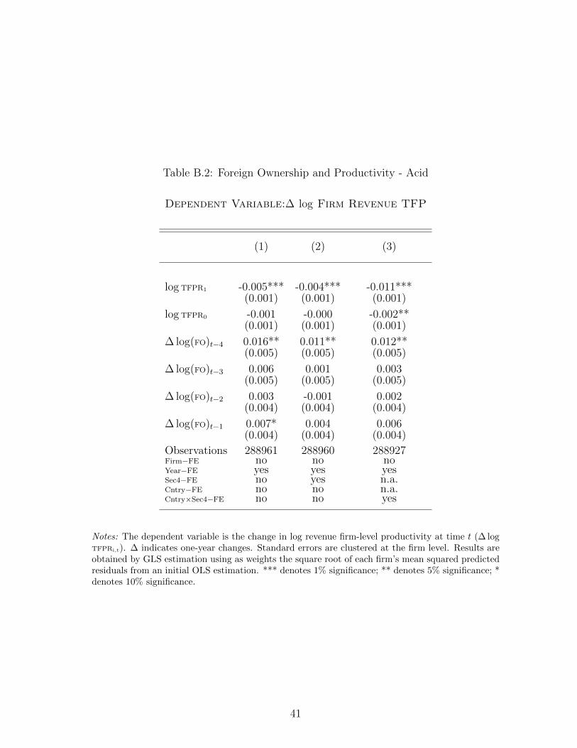
Table B.2: Foreign Ownership and Productivity - Acid

Dependent Variable:∆ log Firm Revenue TFP

(1) (2) (3)

log TFPR1 -0.005*** -0.004*** -0.011***(0.001) (0.001) (0.001)

log TFPR0 -0.001 -0.000 -0.002**(0.001) (0.001) (0.001)

∆ log(FO)t−4 0.016** 0.011** 0.012**(0.005) (0.005) (0.005)

∆ log(FO)t−3 0.006 0.001 0.003(0.005) (0.005) (0.005)

∆ log(FO)t−2 0.003 -0.001 0.002(0.004) (0.004) (0.004)

∆ log(FO)t−1 0.007* 0.004 0.006(0.004) (0.004) (0.004)

Observations 288961 288960 288927Firm−FE no no noYear−FE yes yes yesSec4−FE no yes n.a.Cntry−FE no no n.a.Cntry×Sec4−FE no no yes

Notes: The dependent variable is the change in log revenue firm-level productivity at time t (∆ logTFPRi,t). ∆ indicates one-year changes. Standard errors are clustered at the firm level. Results areobtained by GLS estimation using as weights the square root of each firm’s mean squared predictedresiduals from an initial OLS estimation. *** denotes 1% significance; ** denotes 5% significance; *denotes 10% significance.

41

Table B.3: Foreign Ownership and Productivity - First Stage

Dependent Variable:log TFPR1

(1) (2) (3)

log TFPR0 0.990*** 0.970*** 0.897***(0.001) (0.001) (0.003)

∆ log(FO)t−4 0.005 0.018* 0.041***(0.010) (0.010) (0.010)

∆ log(FO)t−3 -0.007 0.007 0.036***(0.014) (0.011) (0.010)

∆ log(FO)t−2 -0.004 0.009 0.029**(0.013) (0.011) (0.010)

∆ log(FO)t−1 -0.002 0.008 0.026**(0.015) (0.013) (0.012)

Observations 288961 288960 288927Firm−FE no no noYear−FE yes yes yesSec4−FE no yes n.a.Cntry−FE no no n.a.Cntry×Sec4−FE no no yes

Notes: The dependent variable is log TFPR1 the log of revenue firm-level productivity at time t = 1(the second year we observe the firm). The instrument is log TFPR0 which corresponds to the logof revenue firm-level productivity at time t = 0 (the first year we observe the firm). ∆ indicatesone-year changes. Standard errors are clustered at the firm level. Results are obtained by GLSestimation using as weights the square root of each firm’s mean squared predicted residuals froman initial OLS estimation. *** denotes 1% significance; ** denotes 5% significance; * denotes 10%significance.

42

Table B.4: Foreign Ownership and Productivity - GLS

Dependent Variable:∆ log Firm Revenue TFP

(1) (2) (3) (4)

∆ log(FO)t−4 0.012** 0.016** 0.011** 0.012**(0.005) (0.005) (0.005) (0.005)

∆ log(FO)t−3 0.002 0.005 0.001 0.003(0.005) (0.005) (0.005) (0.005)

∆ log(FO)t−2 -0.000 0.003 -0.001 0.002(0.004) (0.004) (0.004) (0.004)

∆ log(FO)t−1 0.004 0.007* 0.004 0.006(0.004) (0.004) (0.004) (0.004)

log TFPR1 -0.006*** -0.004*** -0.013***(0.000) (0.000) (0.000)

Observations 288961 288961 288960 288927Firm−FE no no no noYear−FE yes yes yes yesSec4−FE no no yes n.a.Cntry−FE no no yes n.a.Cntry×Sec4−FE no no no yes

Notes: The dependent variable is the change in log revenue firm-level productivity at time t (∆ logTFPRi,t). ∆ indicates one-year changes. Standard errors are clustered at the firm level. Results areobtained by GLS estimation using as weights the square root of each firm’s mean squared predictedresiduals from an initial OLS estimation. *** denotes 1% significance; ** denotes 5% significance; *denotes 10% significance.

43

Table B.5: Foreign Ownership and Productivity (Majority Ownership and InitialProductivity Only)

Dependent Variable:∆ log Firm Revenue TFP

(1) (2) (3) (4)

∆DFOmajt−4 0.009** 0.011*** 0.009** 0.009**

(0.003) (0.003) (0.003) (0.003)

∆DFOmajt−3 0.002 0.004 0.001 0.002

(0.003) (0.003) (0.003) (0.003)

∆DFOmajt−2 0.000 0.002 -0.001 0.001

(0.003) (0.003) (0.003) (0.003)

∆DFOmajt−1 0.002 0.003 0.001 0.002

(0.003) (0.003) (0.003) (0.003)

log TFPR1 -0.006*** -0.004*** -0.013***(0.000) (0.000) (0.000)

Observations 288927 288927 288927 288927Firm−FE no no no noYear−FE yes yes yes yesSec4−FE no no yes n.a.Cntry−FE no no yes n.a.Cntry×Sec4−FE no no no yes

First Stage-F 298244 86590 20825

Notes: The dependent variable is log revenue firm-level productivity at time t (log TFPRi,t). Standarderrors are clustered at the firm level. Results are obtained by GLS-IV estimation using as weightsthe square root of each firm’s mean squared predicted residuals from an initial OLS-IV estimation.*** denotes 1% significance; ** denotes 5% significance; * denotes 10% significance.

44

Table B.6: Foreign Ownership and Firm Characteristics - Logit Regression

Dependent Variable:Dummy Foreign Ownership

(1)

log L 0.606***(0.148)

log L2 -0.042**

(0.016)

log W 0.614***(0.075)

log VAL 0.311***(0.061)

log KL 0.061**(0.024)

log ASSETS 2.817***(0.370)

log ASSETS2 -0.072***

(0.011)

AGE 0.002*(0.001)

AGE2 -0.000

(0.000)

Observations 84118Sec2−FE yesCntry−FE yes

Notes: The dependent variable is a dummy variable that takes the value of one if the firm everbecomes foreign owned during the sample period (1999-2012). Data included in the estimationrefers only to the first year we observe the firm. Results are obtained by a logit regression. Theobservable variables included are: log employment (log L), log employment squared, log value addedper employee (log VAL), log capital stock per employee (log KL), log assets (log ASSETS), log assetssquared, age (AGE), age squared, wage (log W, which refers to compensation divided by number ofemployees). *** denotes 1% significance; ** denotes 5% significance; * denotes 10% significance.

45

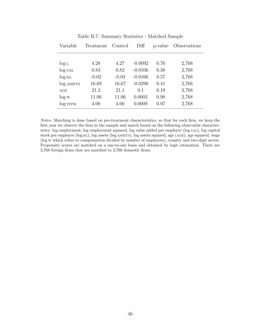
Table B.7: Summary Statistics - Matched Sample

Variable Treatment Control Diff p-value Observations

log L 4.28 4.27 -0.0092 0.76 2,768

log VAL 0.83 0.82 -0.0106 0.38 2,768

log KL -0.02 -0.03 -0.0166 0.57 2,768

log ASSETS 16.69 16.67 -0.0290 0.41 2,768

AGE 21.2 21.1 0.1 0.18 2,768

log W 11.06 11.06 0.0003 0.98 2,768

log TFPR 4.00 4.00 0.0009 0.97 2,768

Notes: Matching is done based on pre-treatment characteristics, so that for each firm, we keep thefirst year we observe the firm in the sample and match based on the following observable character-istics: log employment, log employment squared, log value added per employee (log VAL), log capitalstock per employee (log KL), log assets (log ASSETS), log assets squared, age (AGE), age squared, wage(log W which refers to compensation divided by number of employees), country and two-digit sector.Propensity scores are matched on a one-to-one basis and obtained by logit estimation. There are2,768 foreign firms that are matched to 2,768 domestic firms.

46

Table B.8: Foreign Ownership and Productivity - Matched Sample Results(Coefficients corresponding to lags t− 1, t− 2 and t− 3 are included butsuppressed from the table)

Dependent Variable:∆ log Firm Revenue TFP

(1) (2) (3) (4)

∆ log(FO)t−4 0.017**(0.007)

∆(DFOmajt−4) 0.014**

(0.004)

∆(DFOmint−4) -0.004

(0.004)

∆(DFOmaj+)t−4 0.015** 0.016***(0.005) (0.004)

∆(DFOmaj−)t−4 0.007(0.012)

log TFPR1 -0.014*** -0.014*** -0.014*** -0.014***(0.002) (0.002) (0.002) (0.002)

Observations 18,488 18,488 18,488 18,488Firm−FE no no no noYear−FE yes yes yes yesSec4−FE yes yes yes yesCntry−FE yes yes yes yesCntry×Sec4−FE yes yes no yes

First Stage F 936 527 528 934

Notes: The dependent variable is the change in log revenue firm-level productivity at time t (∆ log TFPRi,t). ∆indicates one-year changes. Standard errors are clustered at the firm level. Results are obtained by GLS-IV estimationusing as weights the square root of each firm’s mean squared predicted residuals from an initial OLS-IV estimation.Matched sample of firms. All columns control for the corresponding t− 1, t− 2 and t− 3 values of the correspondingregressor, but these coefficients are not reported for ease of exposition. Columns (1) to (4) show our baseline resultswith various definitions of foreign ownership. In column (1), ∆ log(FO) refers to the yearly change in the log(FO + 1)where FO is the percentage of foreign ownership. In column (2), DFOmaj is a dummy variable that equals one if thepercentage of foreign ownership is equal or greater than 50%. DFOmin is a dummy variable that equals one if thepercentage of foreign ownership is lower than 50% but greater than 0. In column (3), DFOmaj− is a dummy variablethat equals minus one if the firm went from foreign majority ownership to minority or domestic ownership. Finally,in column (4), DFOmaj+ is a dummy variable that equals one if the firm went from minority or domestically ownedto majority owned (i.e., majority refers to 50 or more percentage ownership). TFPR1: productivity of the firm thesecond time we observe the firm in the sample. *** denotes 1% significance; ** denotes 5% significance; * denotes10% significance.

47

C Production Function Estimation

C.1 Methodology

To obtain firm-level productivity estimates, we estimate the log-value added produc-

tion function

yit = β0 + β``it + βkkit + ωit + εit , (C.1)

where yit is the logarithm of real output, `it is the logarithm of labor input, kit is the

logarithm of capital input, ωit is the logarithm of physical productivity, and εit is a

production shock that is not observable by the firm before making their input deci-

sions at time t. The main concern, when estimating output elasticities with respect

to the inputs in equation (C.1), is whether the firm observes its own productivity ωit

at the time of making input choices. This would render input quantities endogenous

to productivity and ordinary least squares (OLS) estimates of β` and βk would be

inconsistent. We follow the approach suggested in Wooldridge (2009), which builds

on previous work by Olley and Pakes. (1996) (OP) and Levinsohn and Petrin (2003)

(LP), which addresses the concerns raised by Ackerberg, Caves, and Frazer (2015),

who argue that if the flexible labor input is chosen as a function of unobserved pro-

ductivity, the coefficient on labor input is not identified in the previous approaches.

The estimation is based on a two-step procedure to achieve consistency of the

coefficient estimates for the inputs of the production function. Wooldridge (2009)

suggests a generalized method of moments estimation of TFPR to overcome some

limitations of OP and LP, including correction for simultaneous determination of

inputs and productivity, no need to maintain constant returns to scale, and robustness

to the Ackerberg, Caves, and Frazer (2015) critique.27 The following discussion is

based on Wooldridge (2009), accommodated to the case of a production functions

with two production inputs (see Wooldridge (2009) for a general discussion).

27Ackerberg, Caves, and Frazer (2015) highlight that if the variable input (labor) is chosen priorto the time when production takes place, the coefficient on variable input is not identified.

48

For firm i in time period t define

yit = α + βllit + βkkit + ωit + eit , (C.2)

where yit, lit, and kit denote the natural logarithm of firm value added, labor (a

variable input), and capital, respectively. The firm-specific error can be decomposed

into a term capturing firm-specific productivity ωit and an additional term that re-

flects measurement error or unexpected productivity shocks eit. We are interested in

estimating ωit.

A key assumption of the OP and LP estimation methods is that for some function

g(., .):

ωit = g(kit,mit) , (C.3)

where mit is a proxy variable (for investment in OP, for intermediate inputs in LP).

Under the assumption,

E(eit|lit, kit,mit) = 0 t = 1, 2, ..., T , (C.4)

substituting equation (C.3) into equation (C.2), we obtain the regression

E(yit|lit, kit,mit) = α + βllit + βkkit + g(kit,mit) (C.5)

≡ βllit + h(kit,mit) ,

where h(kit,mit) ≡ α + βkkit + g(kit,mit).

In order to identify βl and βk, we need some additional assumptions. First, rewrite

equation (C.4) in a form allowing for more lags:

E(eit|lit, kit,mit, li,t−1, ki,t−1,mi,t−1, ..., li1, ki1,mi1) = 0 t = 1, 2, ..., T . (C.6)

Second, assume productivity follows a first-order Markov process:

E(ωit|ωi,t−1, ..., ωi1) = E(ωit|ωi,t−1) t = 2, 3, ..., T, (C.7)

49

and assume that the productivity innovation ait ≡ ωit − E(ωit|ωi,t−1) is uncorrelated

with current values of the state variable kit as well as past values of the variable input

l, the state k, and the proxy variables m:

E(ωit|kit, li,t−1, ki,t−1,mi,t−1, ..., li1, ki1,mi1) (C.8)

= E(ωit|ωi,t−1) ≡ f [g(ki,t−1,mi,t−1)] .

Recall from equation((C.3)) that ωi,t−1 = g(ki,t−1,mi,t−1).

Plugging ωi,t = f [g(ki,t−1,mi,t−1)] + ait into equation (C.2) gives:

yit = α + βllit + βkkit + f [g(ki,t−1,mi,t−1)] + ait + eit . (C.9)

Now it is possible to specify two equations which identify (βl, βk):

yit = α + βllit + βkkit + g(ki,t,mi,t) + eit (C.10)

and

yit = α + βllit + βkkit + f [g(ki,t−1,mi,t−1)] + uit , (C.11)

where uit ≡ ait + eit.

Important for the GMM estimation strategy, the available orthogonality con-

ditions differ across these two equations. The orthogonality conditions for equa-

tion (C.10) are those outlined in equation (C.6), while the orthogonality conditions

for equation (C.11) are

E(uit|kit, li,t−1, ki,t−1,mi,t−1, ..., li1, ki1,mi1) = 0 t = 2, ..., T . (C.12)

To proceed with the estimation, we estimate these equations parametrically. We

follow Petrin, Reiter, and White (2011) and use a third-degree polynomial approxi-

mation using first order lags of variable input as instruments.28

28We use the Stata routine suggested in Petrin, Reiter, and White (2011).

50

C.2 Estimation Results

Table C.1 reports summary statistics for the output elasticities estimated using the

Wooldridge (2009) approach. The results are consistent across countries with no ma-

jor differences except for Belgium, where the number of observations is slightly lower

and the coefficient on labor is on average marginally lower (0.625) and the average

coefficient on capital marginally higher (0.102).29 Summary statistics are computed

excluding sectors in which the WLP procedure delivers either missing, negative, or

zero coefficients. These cases are few and mainly correspond to sectors 12 “Man-

ufacture of Tobacco products” and 19 “Manufacture of coke and refined petroleum

products,” which have very few observations and contribute little to overall manufac-

turing output.

Table C.1: Summary Statistics of the Production Function Output Elasticities

Labor Elasticity (β`) Capital Elasticity (βk)

Mean 0.734 0.081Median 0.730 0.078Standard Deviation 0.059 0.023Max 0.919 0.338Min 0.453 0.003

29Similarly, the average coefficient on capital is slightly higher in Germany (0.102).

51