chemistry 232. physical chemistry ii · 2020-01-06 · thomas engel and philip reid available with...
TRANSCRIPT
Instructor: Derek Leaist ([email protected])
Office PSC 3072, Lab PSC 3020
Lectures: Monday 8:15 am, Tuesday 10:15 am, Thursday 9:15 am
(MULH 3030)
Lab/Tutorial: Friday 2:15 pm (Lab PSC 3037 / Tutorial PSC 1072)
Course Notes: https://people.stfx.ca/dleaist/Chem232/
(tutorial problems and answers, problem assignments and tests from
2016-2019, equations sheets, and reading material also posted)
Textbook: Thermodynamics, Statistical Thermodynamics and
(optional) Kinetics, 3rd Edition, Thomas Engel and Philip Reid
Chemistry 232. Physical Chemistry II
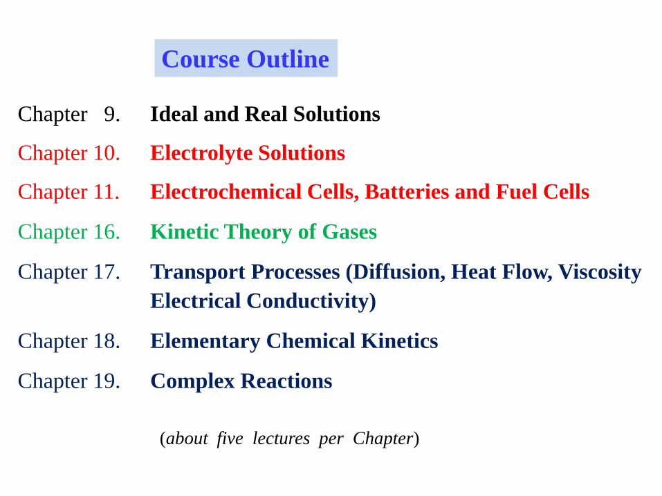
Chapter 9. Ideal and Real Solutions
Chapter 10. Electrolyte Solutions
Chapter 11. Electrochemical Cells, Batteries and Fuel Cells
Chapter 16. Kinetic Theory of Gases
Chapter 17. Transport Processes (Diffusion, Heat Flow, Viscosity
Electrical Conductivity)
Chapter 18. Elementary Chemical Kinetics
Chapter 19. Complex Reactions
Course Outline
(about five lectures per Chapter)
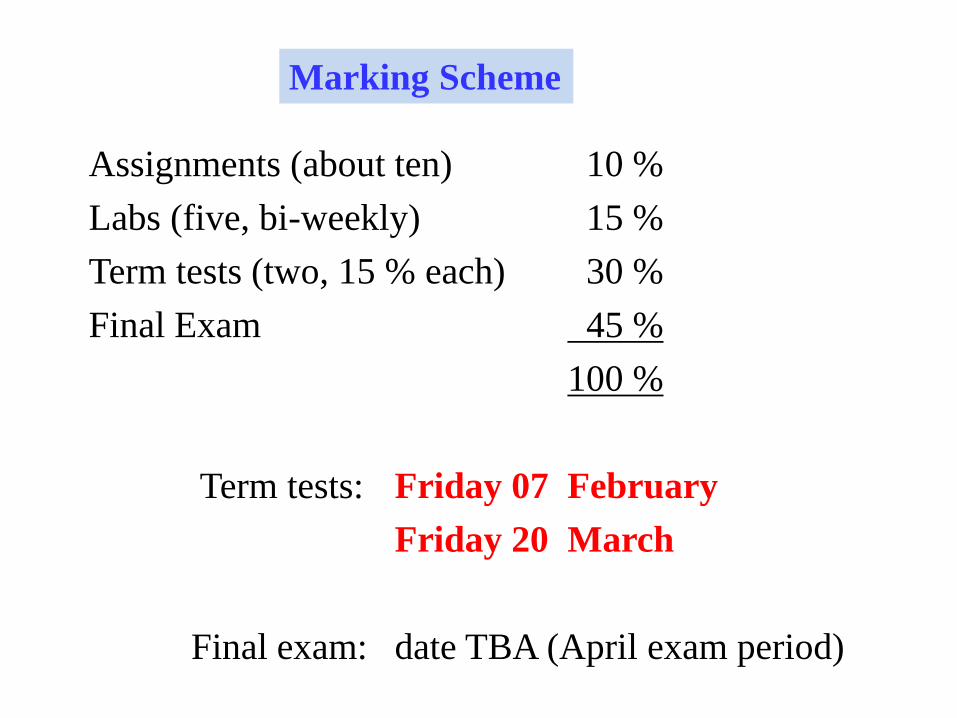
Assignments (about ten) 10 %
Labs (five, bi-weekly) 15 %
Term tests (two, 15 % each) 30 %
Final Exam 45 %
100 %
Term tests: Friday 07 February
Friday 20 March
Final exam: date TBA (April exam period)
Marking Scheme
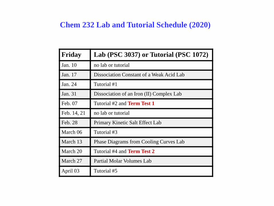
Friday Lab (PSC 3037) or Tutorial (PSC 1072)
Jan. 10 no lab or tutorial
Jan. 17 Dissociation Constant of a Weak Acid Lab
Jan. 24 Tutorial #1
Jan. 31 Dissociation of an Iron (II) Complex Lab
Feb. 07 Tutorial #2 and Term Test 1
Feb. 14, 21 no lab or tutorial
Feb. 28 Primary Kinetic Salt Effect Lab
March 06 Tutorial #3
March 13 Phase Diagrams from Cooling Curves Lab
March 20 Tutorial #4 and Term Test 2
March 27 Partial Molar Volumes Lab
April 03 Tutorial #5
Chem 232 Lab and Tutorial Schedule (2020)
Textbook (optional)
(for Chem 231 and Chem 232)
Thermodynamics, Statistical
Thermodynamics and Kinetics
3rd Edition ($126 Amazon.ca)
Thomas Engel and Philip Reid
available with “free” online
Mastering Chemistry resource
material
or Physical Chemistry, 3rd Edition,
Thomas Engel and Philip Reid
includes chapters on quantum mechanics and
spectroscopy for Chemistry 331 and 332
(but not required for these courses)
Same textbook used previously.
Used copies may be available.
Also available online:https://www.academia.edu/14903550/Thermodynamics_Statistical_Thermodynamics_and_Kinetics_THIRD_EDITION
Student Solutions Manual
(for Chem 231 and Chem 232)
Thermodynamics, Statistical
Thermodynamics and Kinetics
3rd Edition ($34 Amazon.ca)
Thomas Engel and Philip Reid
worked solutions to
end-of-chapter problems
Schaum’s Outline of Physical Chemistry
2nd edition ($25 Amazon.ca)
Clyde A. Metz
Thermodynamics, electrochemistry,
kinetics, and transport properties
for Chem 231 and Chem 232.
concise summaries, worked problems.
Also covers: quantum mechanics
spectroscopy
crystallography
polymers
Chem 232: Course Material
https://people.stfx.ca/dleaist/Chem232/
lab and tutorial schedule
course notes
tutorial problems with answers
problem sets with answers from 2016, 2017, 2018, 2019
term tests with answers from 2016, 2017, 2018, 2019
equation sheets
pdf copy of the textbook: T. Engel, P. Reid, Thermodynamics, Statistical
Thermodynamics and Kinetics, 3rd Ed., Pearson, Boston, 2013.
Chapter 9. Ideal and Real Solutions
Chem 231 Last term, thermodynamics of pure substances and ideal gas mixtures. But what about liquid mixtures? They are “everywhere”, very important, and often strongly nonideal.
Solutions
mixtures of two or more different chemical components
form a single phase
uniform chemical and physical properties on the microscopic scale
a solution can be a: gas (e.g., air – N2, O2, H2O, Ar, CO2, …)
liquid (e.g., NaCl dissolved in water)
solid (e.g., brass – a copper/zinc alloy)
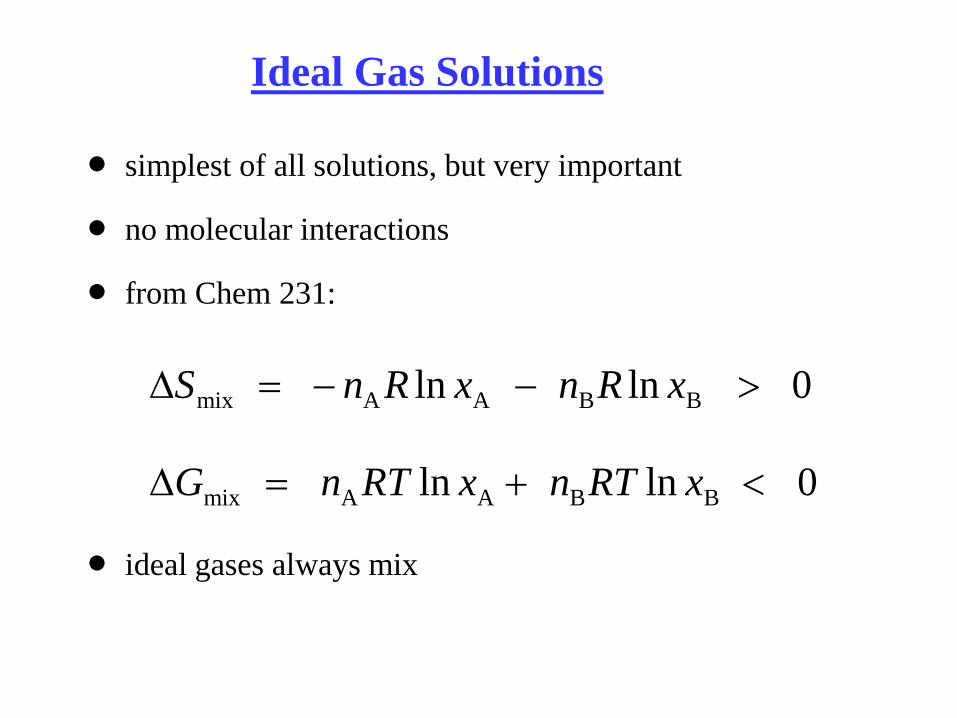
Ideal Gas Solutions
simplest of all solutions, but very important
no molecular interactions
from Chem 231:
ideal gases always mix
0lnln BBAAmix xRnxRnS
0lnln BBAAmix xRTnxRTnG
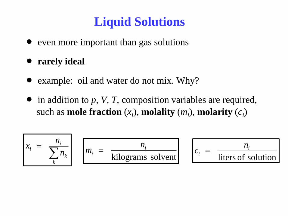
Liquid Solutions
even more important than gas solutions
rarely ideal
example: oil and water do not mix. Why?
in addition to p, V, T, composition variables are required,
such as mole fraction (xi), molality (mi), molarity (ci)
k
k
ii
n
nx
solvent kilograms
ii
nm
solution of liters
ii
nc
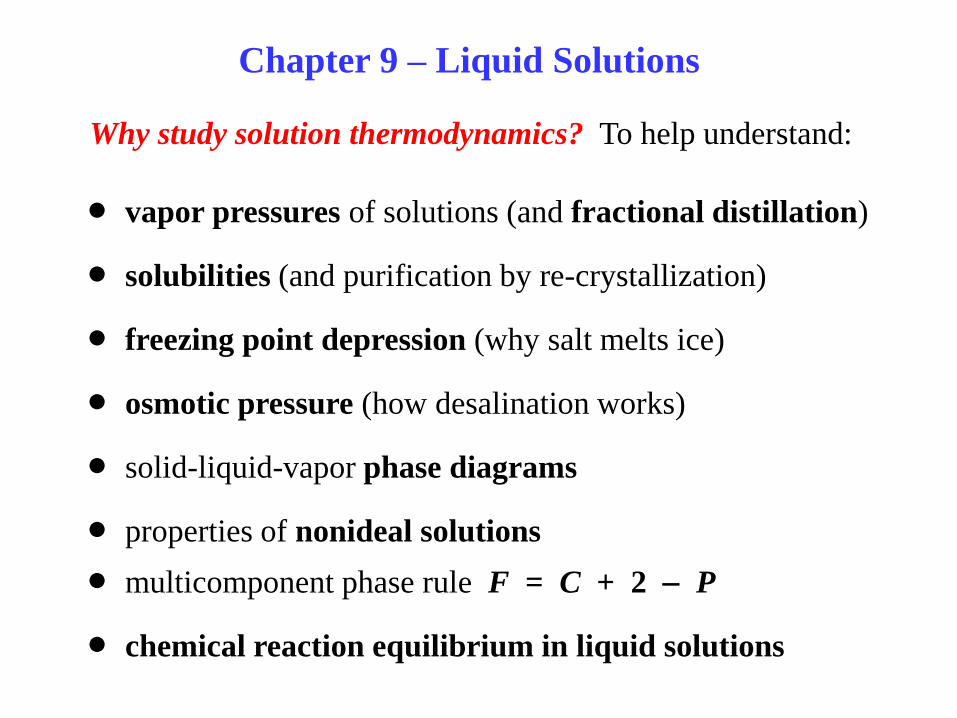
Chapter 9 – Liquid Solutions
Why study solution thermodynamics? To help understand:
vapor pressures of solutions (and fractional distillation)
solubilities (and purification by re-crystallization)
freezing point depression (why salt melts ice)
osmotic pressure (how desalination works)
solid-liquid-vapor phase diagrams
properties of nonideal solutions
multicomponent phase rule F = C + 2 P
chemical reaction equilibrium in liquid solutions
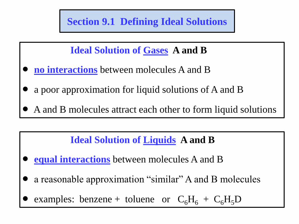
Ideal Solution of Gases A and B
no interactions between molecules A and B
a poor approximation for liquid solutions of A and B
A and B molecules attract each other to form liquid solutions
Section 9.1 Defining Ideal Solutions
Ideal Solution of Liquids A and B
equal interactions between molecules A and B
a reasonable approximation “similar” A and B molecules
examples: benzene + toluene or C6H6 + C6H5D
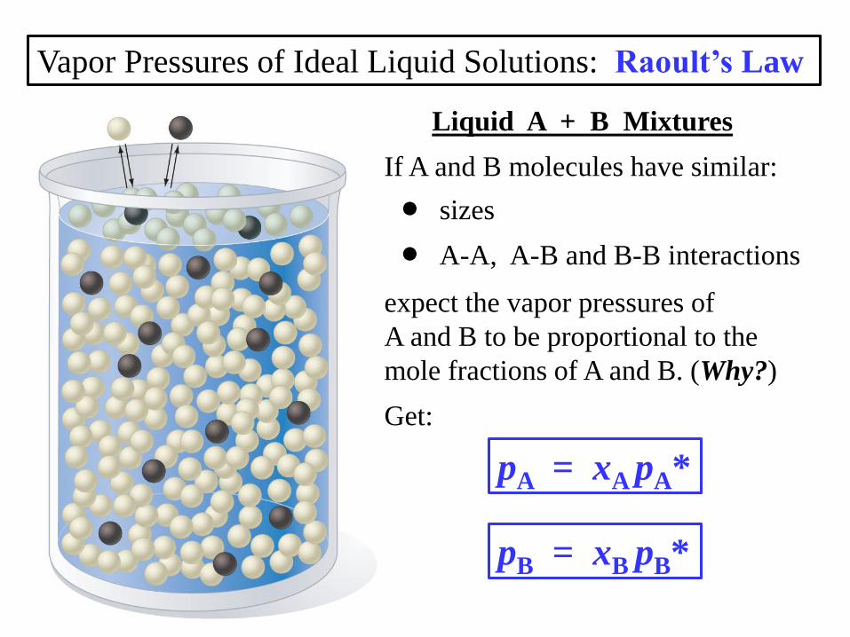
Vapor Pressures of Ideal Liquid Solutions: Raoult’s Law
Liquid A + B Mixtures
If A and B molecules have similar:
sizes
A-A, A-B and B-B interactions
expect the vapor pressures of
A and B to be proportional to the
mole fractions of A and B. (Why?)
Get:
pA = xA pA*
pB = xB pB*
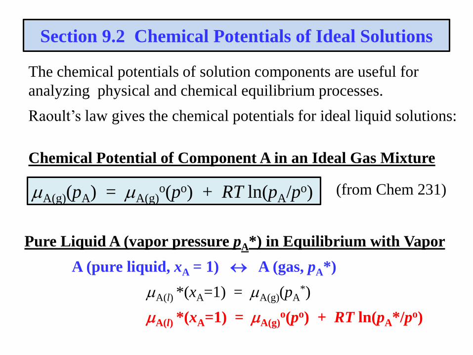
Section 9.2 Chemical Potentials of Ideal Solutions
The chemical potentials of solution components are useful for
analyzing physical and chemical equilibrium processes.
Raoult’s law gives the chemical potentials for ideal liquid solutions:
Chemical Potential of Component A in an Ideal Gas Mixture
(from Chem 231)
Pure Liquid A (vapor pressure pA*) in Equilibrium with Vapor
A (pure liquid, xA = 1) A (gas, pA*)
A(l) *(xA=1) = A(g)(pA*)
A(l) *(xA=1) = A(g)o(po) + RT ln(pA*/po)
A(g)(pA) = A(g)o(po) + RT ln(pA/po)
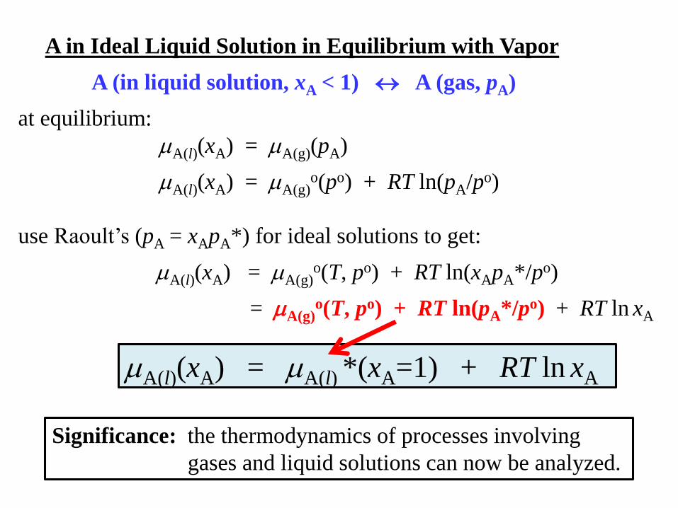
A in Ideal Liquid Solution in Equilibrium with Vapor
A (in liquid solution, xA < 1) A (gas, pA)
at equilibrium:
A(l)(xA) = A(g)(pA)
A(l)(xA) = A(g)o(po) + RT ln(pA/po)
use Raoult’s (pA = xApA*) for ideal solutions to get:
A(l)(xA) = A(g)o(T, po) + RT ln(xApA*/po)
= A(g)o(T, po) + RT ln(pA*/po) + RT ln xA
A(l)(xA) = A(l) *(xA=1) + RT ln xA
Significance: the thermodynamics of processes involving
gases and liquid solutions can now be analyzed.
Ideal Liquid Solutions
Example nA moles of pure liquid A and nB moles of pure
liquid B are mixed at temperature T to form an
ideal liquid solution. Exercise Show:
0lnln BBAAmix xRnxRnS
0lnln BBAAmix xRTnxRTnG
Identical results for mixing ideal gases at fixed T and p.
Why is it unnecessary to specify the pressure for mixing liquids?
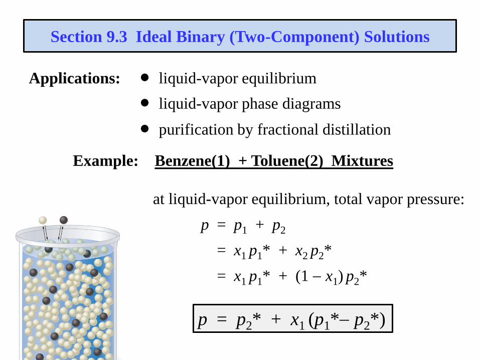
Section 9.3 Ideal Binary (Two-Component) Solutions
Applications: liquid-vapor equilibrium
liquid-vapor phase diagrams
purification by fractional distillation
Example: Benzene(1) + Toluene(2) Mixtures
at liquid-vapor equilibrium, total vapor pressure:
p = p1 + p2
= x1 p1* + x2 p2*
= x1 p1* + (1 x1) p2*
p = p2* + x1 (p1* p2*)
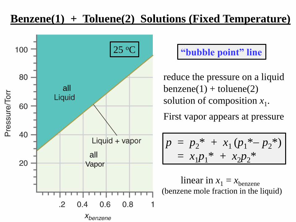
Benzene(1) + Toluene(2) Solutions (Fixed Temperature)
p = p2* + x1 (p1* p2*)
= x1p1* + x2p2*
all
linear in x1 = xbenzene
(benzene mole fraction in the liquid)
allVapor
reduce the pressure on a liquid
benzene(1) + toluene(2)
solution of composition x1.
First vapor appears at pressure
“bubble point” line25 oC
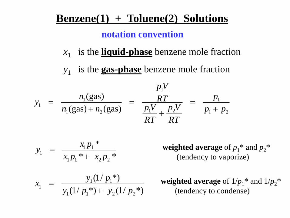
Benzene(1) + Toluene(2) Solutions
notation convention
x1 is the liquid-phase benzene mole fraction
y1 is the gas-phase benzene mole fraction
21
1
21
1
21
11
)gas()gas(
)gas(
pp
p
RT
Vp
RT
VpRT
Vp
nn
ny
**
*
2211
111
pxpx
pxy
*)/1(*)/1(
*)/1(
2211
111
pypy
pyx
weighted average of p1* and p2*
(tendency to vaporize)
weighted average of 1/p1* and 1/p2*
(tendency to condense)
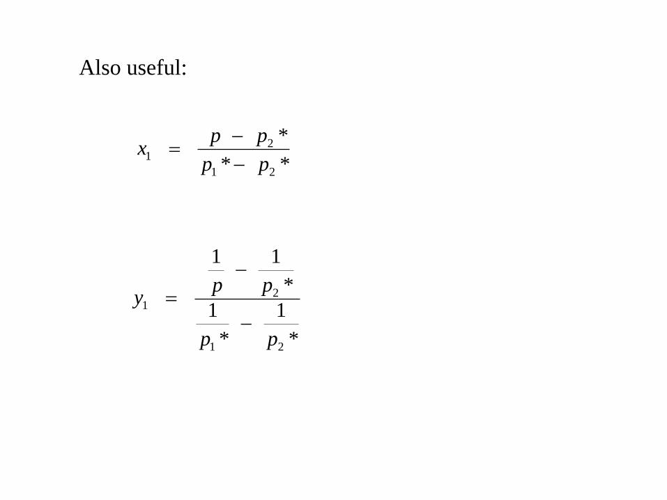
Also useful:
**
*
21
21
pp
ppx
*
1
*
1
*
11
21
21
pp
ppy
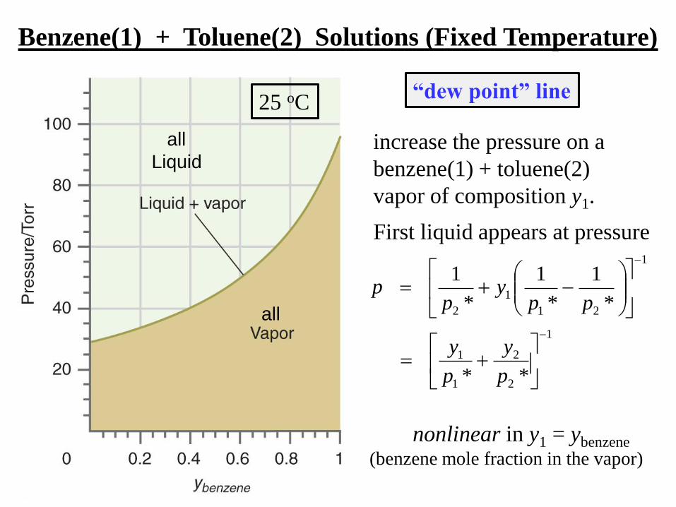
Benzene(1) + Toluene(2) Solutions (Fixed Temperature)
all
Liquid
nonlinear in y1 = ybenzene
(benzene mole fraction in the vapor)
all
increase the pressure on a
benzene(1) + toluene(2)
vapor of composition y1.
First liquid appears at pressure
“dew point” line
1
2
2
1
1
1
21
1
2
**
*
1
*
1
*
1
p
y
p
y
ppy
pp
25 oC
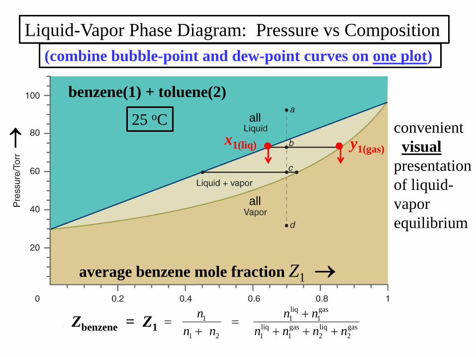
Liquid-Vapor Phase Diagram: Pressure vs Composition
(combine bubble-point and dew-point curves on one plot)
25 oC
Zbenzene = Z1
benzene(1) + toluene(2)
gas
2
liq
2
gas
1
liq
1
gas
1
liq
1
21
1
nnnn
nn
nn
n
convenient
visual
presentation
of liquid-
vapor
equilibrium
all
all
average benzene mole fraction Z1
y1(gas)x1(liq)
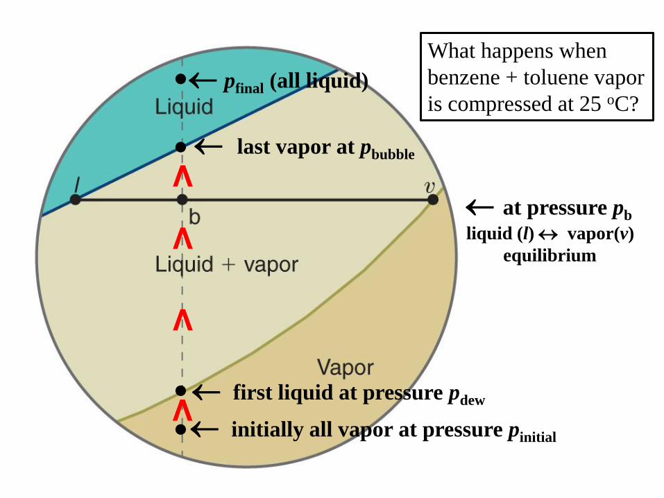
What happens when
benzene + toluene vapor
is compressed at 25 oC?
initially all vapor at pressure pinitial
pfinal (all liquid)
last vapor at pbubble
first liquid at pressure pdew
at pressure pb
liquid (l) vapor(v)
equilibrium
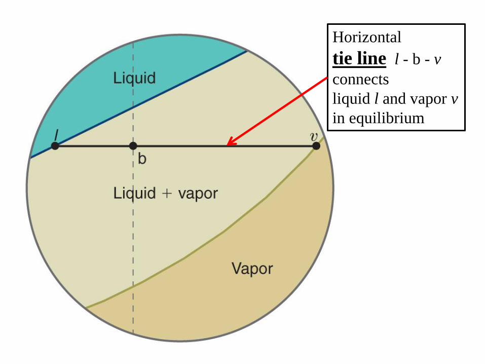
Horizontal
tie line l - b - v
connects
liquid l and vapor v
in equilibrium
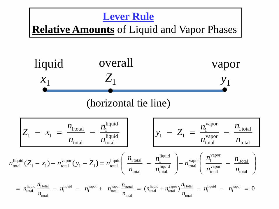
Lever Rule
Relative Amounts of Liquid and Vapor Phases
liquid
x1
vapor
y1
overall
Z1
(horizontal tie line)
liquid
total
liquid
1
total
total1
11n
n
n
nxZ
total
total1
vapor
total
vapor
111
n
n
n
nZy
total
total1
vapor
total
vapor
1vapor
totalliquid
total
liquid
1
total
total1liquid
total11
vapor
total11
liquid
total )()(n
n
n
nn
n
n
n
nnZynxZn
0)( vapor
1
liquid
1
total
total1vapor
total
liquid
total
total
total1vapor
total
vapor
1
liquid
1
total
total1liquid
total nnn
nnn
n
nnnn
n
nn
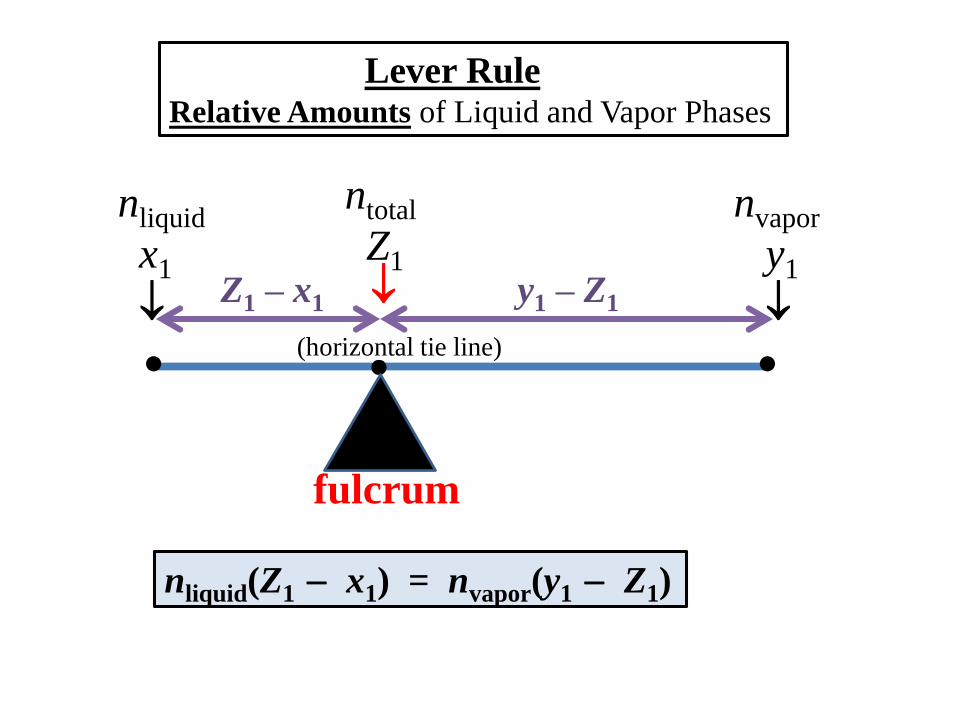
Lever RuleRelative Amounts of Liquid and Vapor Phases
nliquid
x1
nvapor
y1
ntotal
Z1
(horizontal tie line)
nliquid(Z1 x1) = nvapor(y1 Z1)
Z1 – x1 y1 – Z1
fulcrum
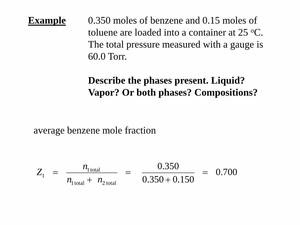
Example 0.350 moles of benzene and 0.15 moles of
toluene are loaded into a container at 25 oC.
The total pressure measured with a gauge is
60.0 Torr.
Describe the phases present. Liquid?
Vapor? Or both phases? Compositions?
average benzene mole fraction
700.0150.0350.0
350.0
total2 total1
total11
nn
nZ
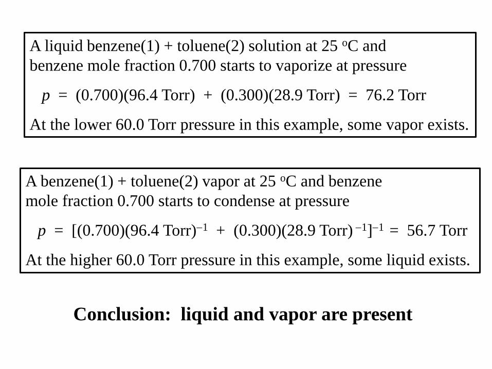
A liquid benzene(1) + toluene(2) solution at 25 oC and
benzene mole fraction 0.700 starts to vaporize at pressure
p = (0.700)(96.4 Torr) + (0.300)(28.9 Torr) = 76.2 Torr
At the lower 60.0 Torr pressure in this example, some vapor exists.
A benzene(1) + toluene(2) vapor at 25 oC and benzene
mole fraction 0.700 starts to condense at pressure
p = [(0.700)(96.4 Torr)1 + (0.300)(28.9 Torr) 1]1 = 56.7 Torr
At the higher 60.0 Torr pressure in this example, some liquid exists.
Conclusion: liquid and vapor are present
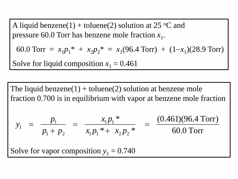
A liquid benzene(1) + toluene(2) solution at 25 oC and
pressure 60.0 Torr has benzene mole fraction x1.
60.0 Torr = x1p1* + x2p2* = x1(96.4 Torr) + (1x1)(28.9 Torr)
Solve for liquid composition x1 = 0.461
The liquid benzene(1) + toluene(2) solution at benzene mole
fraction 0.700 is in equilibrium with vapor at benzene mole fraction
Solve for vapor composition y1 = 0.740
Torr0.60
)Torr4.96)(461.0(
**
*
2211
11
21
11
pxpx
px
pp
py
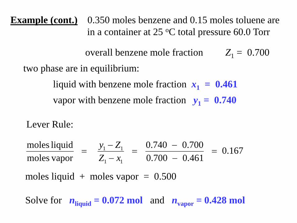
Example (cont.) 0.350 moles benzene and 0.15 moles toluene are
in a container at 25 oC total pressure 60.0 Torr
overall benzene mole fraction Z1 = 0.700
two phase are in equilibrium:
liquid with benzene mole fraction x1 = 0.461
vapor with benzene mole fraction y1 = 0.740
167.0461.0700.0
700.0740.0
vapormoles
liquid moles
11
11
xZ
Zy
Lever Rule:
moles liquid + moles vapor = 0.500
Solve for nliquid = 0.072 mol and nvapor = 0.428 mol
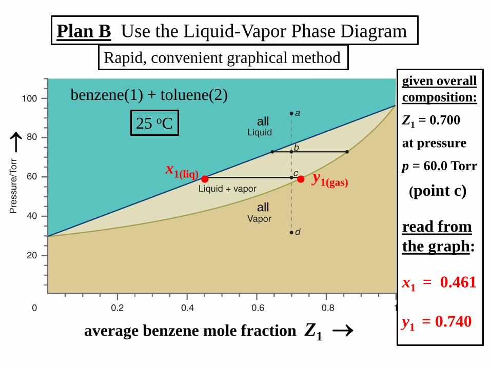
Plan B Use the Liquid-Vapor Phase Diagram
Rapid, convenient graphical method
25 oC
benzene(1) + toluene(2)
all
all
average benzene mole fraction Z1
y1(gas)
x1(liq)
given overall
composition:
Z1 = 0.700
at pressure
p = 60.0 Torr
(point c)
read from
the graph:
x1 = 0.461
y1 = 0.740
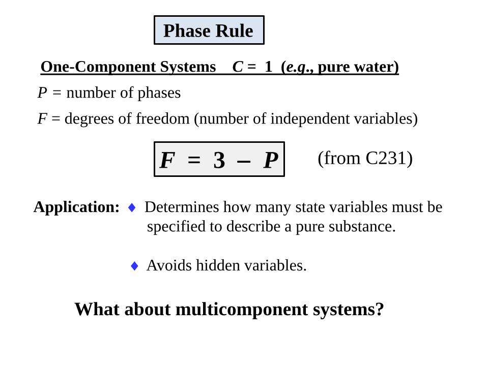
Phase Rule
One-Component Systems C = 1 (e.g., pure water)
P = number of phases
F = degrees of freedom (number of independent variables)
(from C231)
Application: Determines how many state variables must be
specified to describe a pure substance.
Avoids hidden variables.
What about multicomponent systems?
F = 3 P
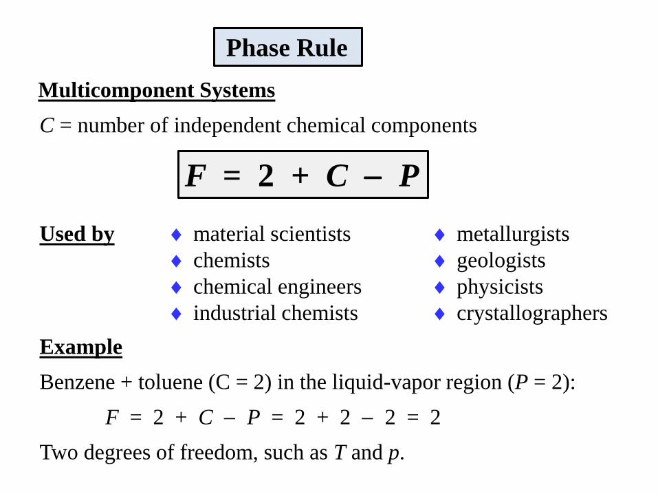
Phase Rule
Multicomponent Systems
C = number of independent chemical components
Example
Benzene + toluene (C = 2) in the liquid-vapor region (P = 2):
F = 2 + C P = 2 + 2 2 = 2
Two degrees of freedom, such as T and p.
F = 2 + C P
Used by material scientists metallurgists
chemists geologists
chemical engineers physicists
industrial chemists crystallographers
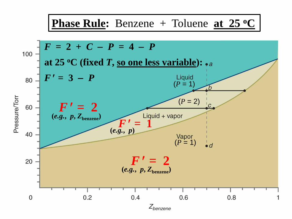
Phase Rule: Benzene + Toluene at 25 oC
F = 2 + C P = 4 P
at 25 oC (fixed T, so one less variable):
F = 3 P
F = 2
F = 2
F = 1 (e.g., p, Zbenzene)
(e.g., p, Zbenzene)
(e.g., p)
(P = 1)
(P = 1)
(P = 2)
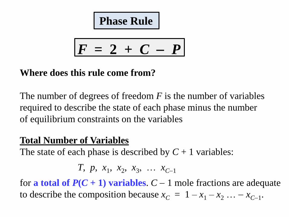
Phase Rule
F = 2 + C P
Where does this rule come from?
The number of degrees of freedom F is the number of variables
required to describe the state of each phase minus the number
of equilibrium constraints on the variables
Total Number of Variables
The state of each phase is described by C + 1 variables:
T, p, x1, x2, x3, … xC1
for a total of P(C + 1) variables. C 1 mole fractions are adequate
to describe the composition because xC = 1 – x1 – x2 … xC1.
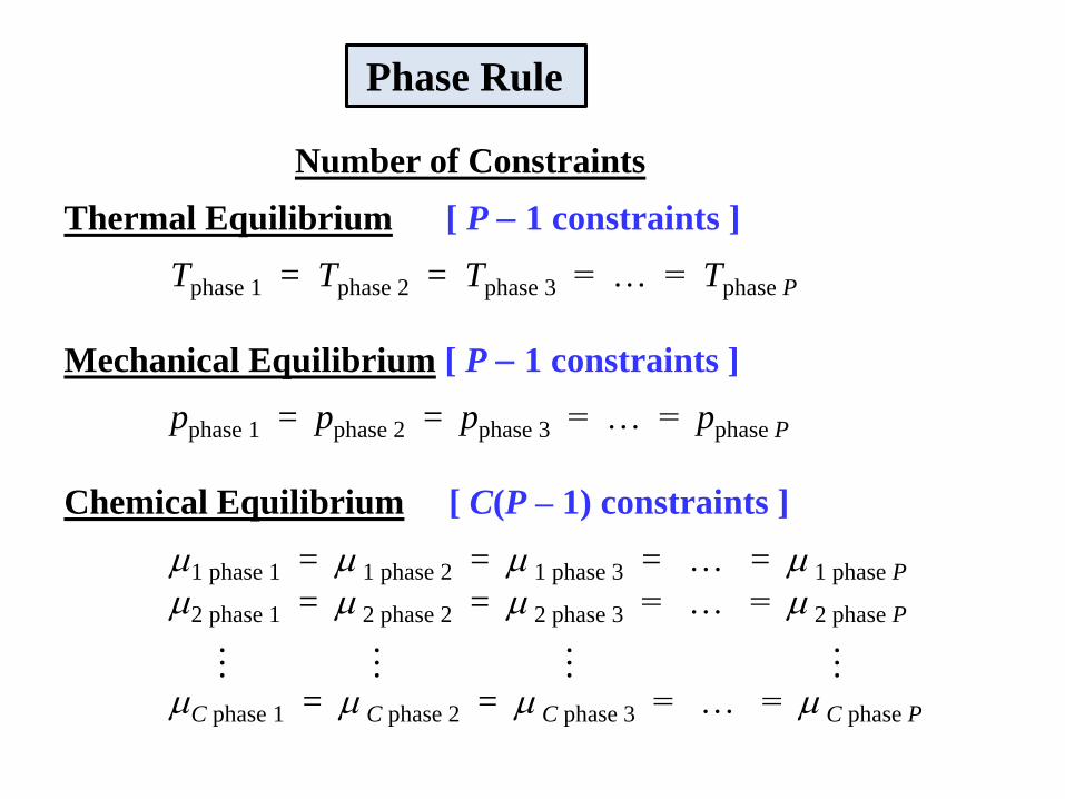
Phase Rule
Number of Constraints
Thermal Equilibrium [ P 1 constraints ]
Tphase 1 = Tphase 2 = Tphase 3 = … = Tphase P
Mechanical Equilibrium [ P 1 constraints ]
pphase 1 = pphase 2 = pphase 3 = … = pphase P
Chemical Equilibrium [ C(P – 1) constraints ]
1 phase 1 = 1 phase 2 = 1 phase 3 = … = 1 phase P
2 phase 1 = 2 phase 2 = 2 phase 3 = … = 2 phase P
C phase 1 = C phase 2 = C phase 3 = … = C phase P
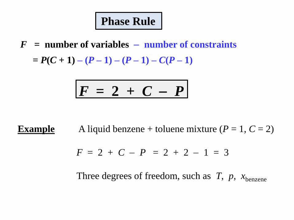
Phase Rule
F = number of variables number of constraints
= P(C + 1) – (P – 1) – (P – 1) – C(P – 1)
F = 2 + C P
Example A liquid benzene + toluene mixture (P = 1, C = 2)
F = 2 + C P = 2 + 2 1 = 3
Three degrees of freedom, such as T, p, xbenzene
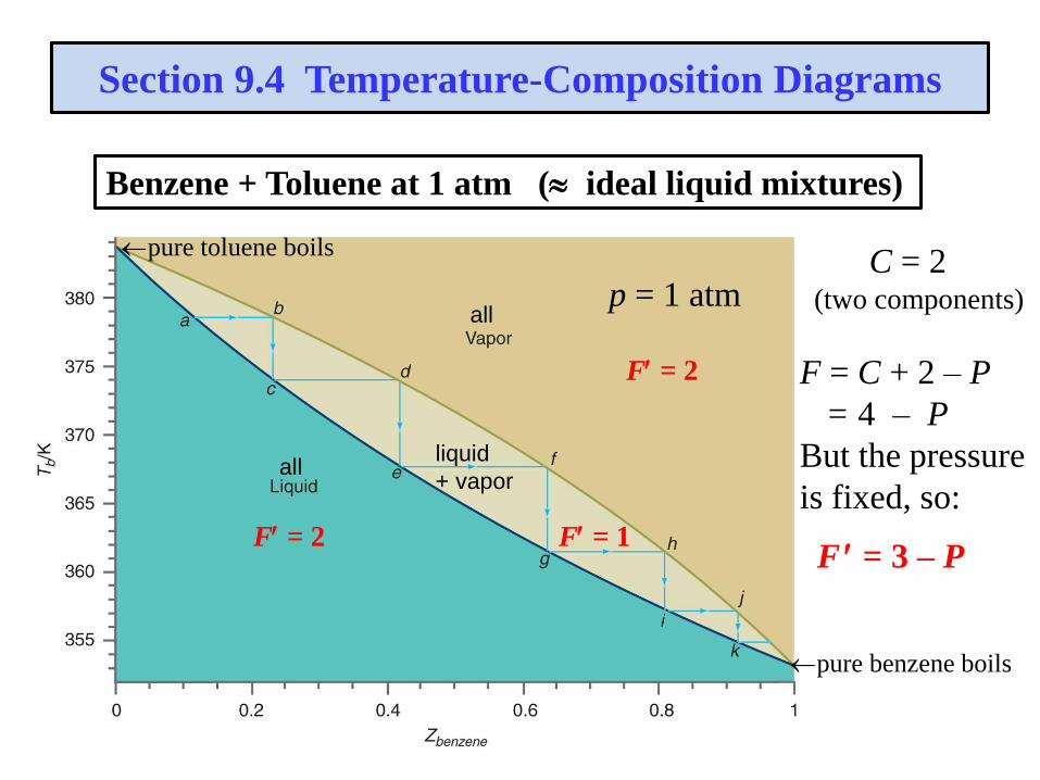
Section 9.4 Temperature-Composition Diagrams
Benzene + Toluene at 1 atm ( ideal liquid mixtures)
all
allliquid
+ vapor
pure benzene boils
pure toluene boils
F = 2
F = 1F = 2
p = 1 atmC = 2
(two components)
F = C + 2 – P
= 4 – P
But the pressure
is fixed, so:
F = 3 – P
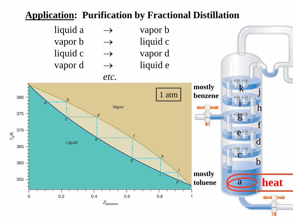
Application: Purification by Fractional Distillation
liquid a vapor b
vapor b liquid c
liquid c vapor d
vapor d liquid e
etc.
a
bc
de
fg
hi
1 atm
mostly
toluene
mostly
benzene
heat
k j
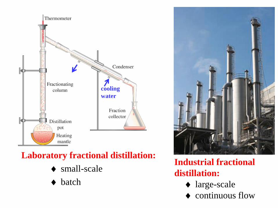
Laboratory fractional distillation:
small-scale
batch
cooling
water
Industrial fractional
distillation:
large-scale
continuous flow
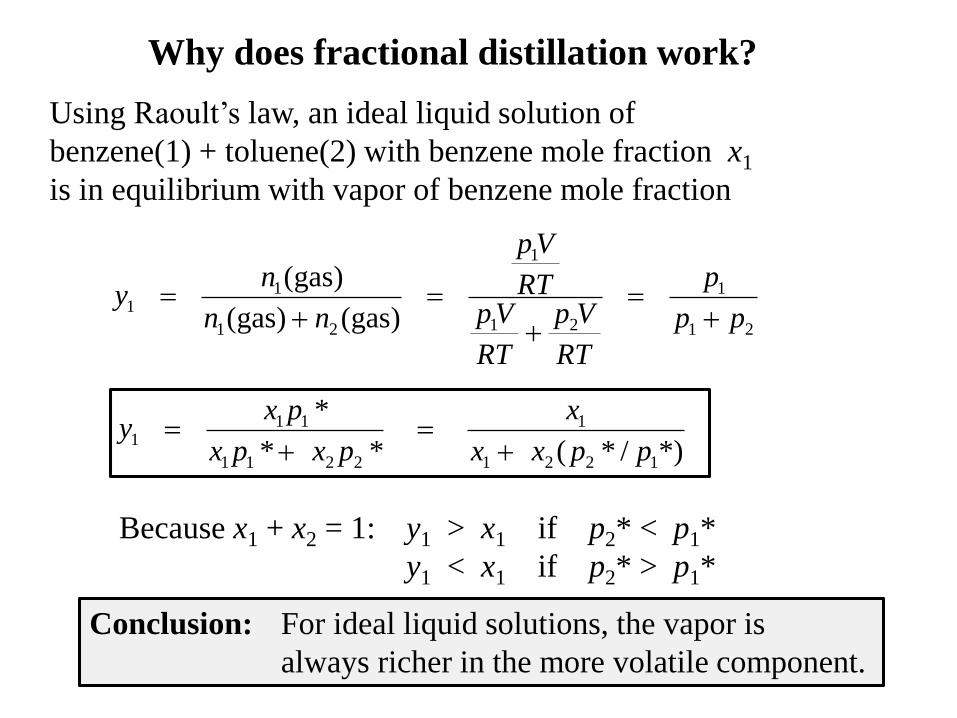
Using Raoult’s law, an ideal liquid solution of
benzene(1) + toluene(2) with benzene mole fraction x1
is in equilibrium with vapor of benzene mole fraction
21
1
21
1
21
11
)gas()gas(
)gas(
pp
p
RT
Vp
RT
VpRT
Vp
nn
ny
*)/*(**
*
1221
1
2211
111
ppxx
x
pxpx
pxy
Why does fractional distillation work?
Because x1 + x2 = 1: y1 > x1 if p2* < p1*
y1 < x1 if p2* > p1*
Conclusion: For ideal liquid solutions, the vapor is
always richer in the more volatile component.
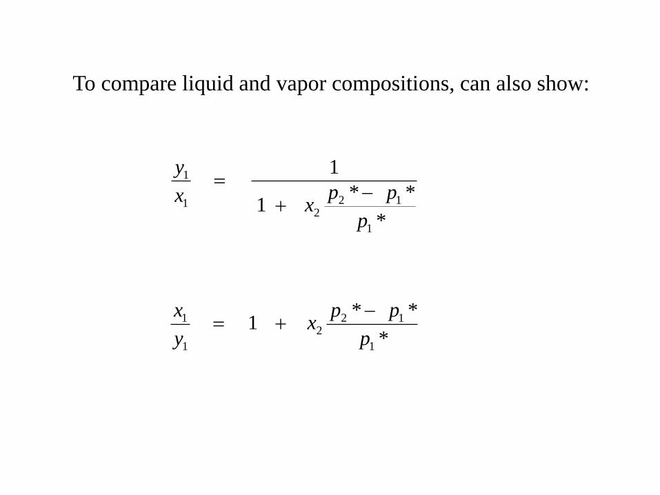
To compare liquid and vapor compositions, can also show:
*
**1
1
1
122
1
1
p
ppx
x
y
*
**1
1
122
1
1
p
ppx
y
x
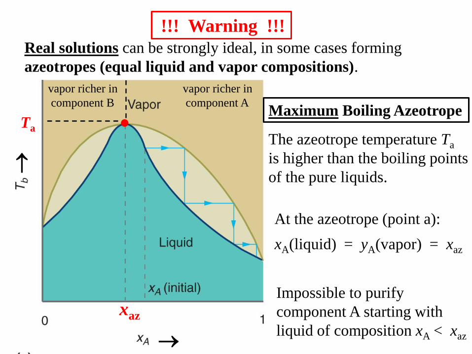
Real solutions can be strongly ideal, in some cases forming
azeotropes (equal liquid and vapor compositions).
!!! Warning !!!
Maximum Boiling Azeotrope
At the azeotrope (point a):
xA(liquid) = yA(vapor) = xaz
The azeotrope temperature Ta
is higher than the boiling points
of the pure liquids.
vapor richer in
component A
vapor richer in
component B
Ta
xaz
Impossible to purify
component A starting with
liquid of composition xA < xaz
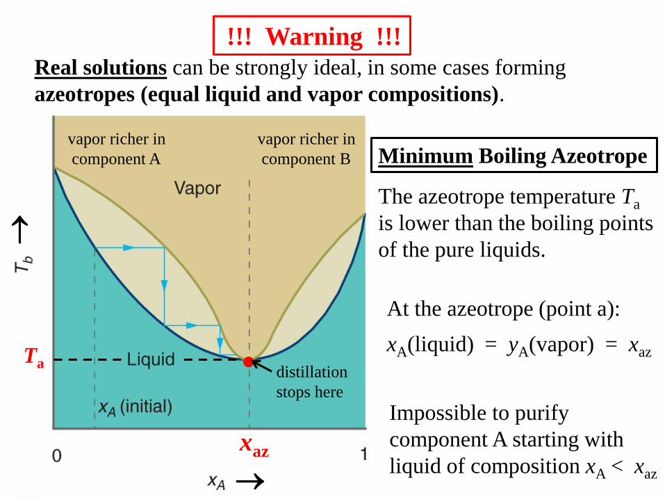
Real solutions can be strongly ideal, in some cases forming
azeotropes (equal liquid and vapor compositions).
!!! Warning !!!
Minimum Boiling Azeotrope
At the azeotrope (point a):
xA(liquid) = yA(vapor) = xaz
The azeotrope temperature Ta
is lower than the boiling points
of the pure liquids.
vapor richer in
component B
vapor richer in
component A
Ta
xaz
Impossible to purify
component A starting with
liquid of composition xA < xaz
distillation
stops here
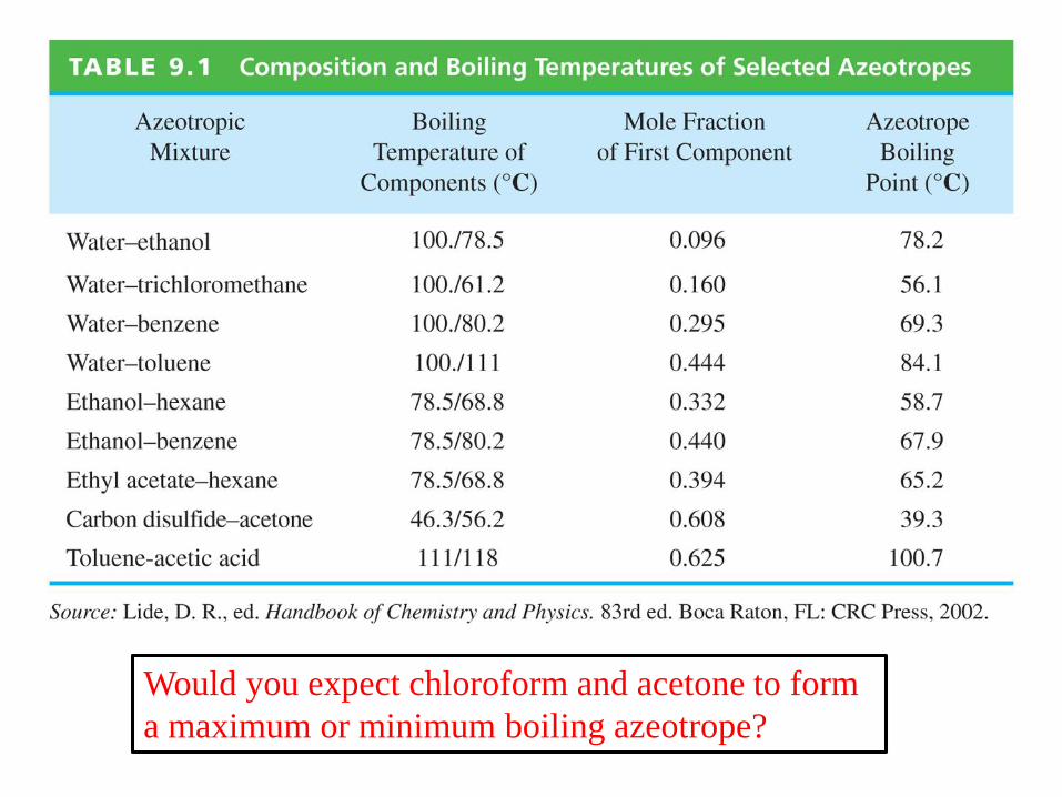
Would you expect chloroform and acetone to form
a maximum or minimum boiling azeotrope?
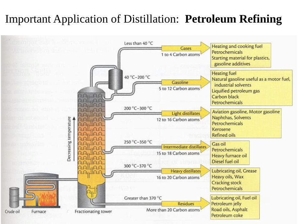
Important Application of Distillation: Petroleum Refining
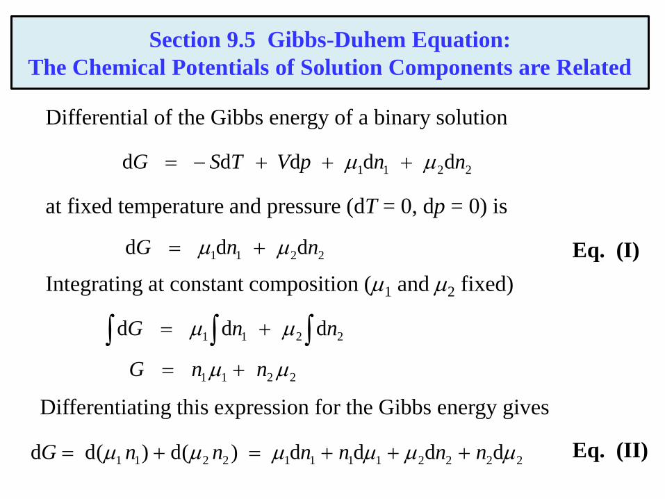
Section 9.5 Gibbs-Duhem Equation:
The Chemical Potentials of Solution Components are Related
Differential of the Gibbs energy of a binary solution
2211 ddddd nnpVTSG
at fixed temperature and pressure (dT = 0, dp = 0) is
2211 ddd nnG
2211 ddd nnG
Integrating at constant composition (1 and 2 fixed)
2211 nnG
Differentiating this expression for the Gibbs energy gives
222211112211 dddd)(d)(dd nnnnnnG
Eq. (I)
Eq. (II)
Gibbs-Duhem Equation:
The Chemical Potentials of Solution Components are Related
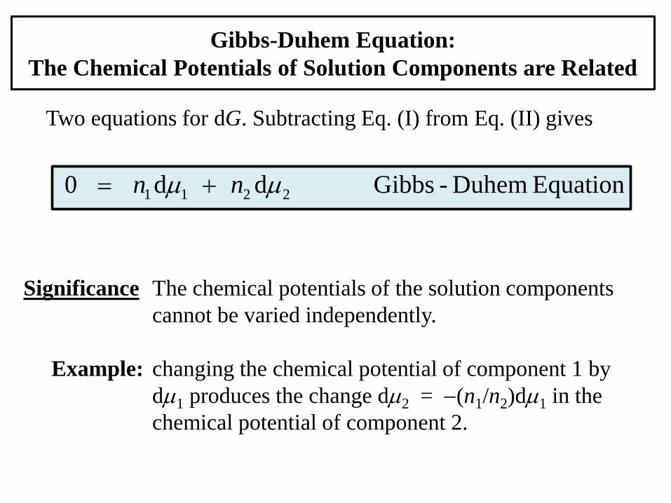
Two equations for dG. Subtracting Eq. (I) from Eq. (II) gives
Equation Duhem-Gibbs dd0 2211 nn
Significance The chemical potentials of the solution components
cannot be varied independently.
Example: changing the chemical potential of component 1 by
d1 produces the change d2 = (n1/n2)d1 in the
chemical potential of component 2.
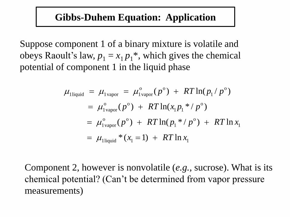
Gibbs-Duhem Equation: Application
Suppose component 1 of a binary mixture is volatile and
obeys Raoult’s law, p1 = x1 p1*, which gives the chemical
potential of component 1 in the liquid phase
11liquid1
1
o
1
oo
vapor1
o
11
oo
vapor1
o
1
oo
vapor1vapor1liquid1
ln)1(*
ln)/*ln()(
)/*ln()(
)/ln()(
xRTx
xRTppRTp
ppxRTp
ppRTp
Component 2, however is nonvolatile (e.g., sucrose). What is its
chemical potential? (Can’t be determined from vapor pressure
measurements)
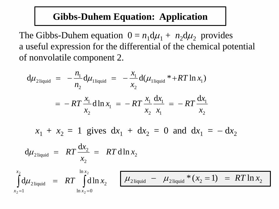
Gibbs-Duhem Equation: Application
The Gibbs-Duhem equation 0 = n1d1 + n2d2 provides
a useful expression for the differential of the chemical potential
of nonvolatile component 2.
)ln*d(dd 1liquid1
2
1liquid1
2
1liquid2 xRT
x
x
n
n
x1 + x2 = 1 gives dx1 + dx2 = 0 and dx1 = dx2
2
1
1
1
2
11
2
1 ddlnd
x
xRT
x
x
x
xRTx
x
xRT
2
2
2liquid2 lnd
dd xRT
x
xRT
2
2
2
2
ln
0ln
2
1
liquid2 lndd
x
x
x
x
xRT 22liquid2liquid2 ln)1(* xRTx
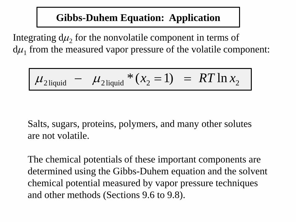
Gibbs-Duhem Equation: Application
Integrating d2 for the nonvolatile component in terms of
d1 from the measured vapor pressure of the volatile component:
22liquid2liquid2 ln)1(* xRTx
Salts, sugars, proteins, polymers, and many other solutes
are not volatile.
The chemical potentials of these important components are
determined using the Gibbs-Duhem equation and the solvent
chemical potential measured by vapor pressure techniques
and other methods (Sections 9.6 to 9.8).
Several important properties of dilute solutions
collectively (leading to the terminology “colligative”)
depend only on the number of solvent and solute molecules,
not on their chemical composition or molecular structure.
vapor pressure lowering
freezing point depression
boiling point elevation
osmotic pressure
Why?
Section 9.6 Colligative Properties
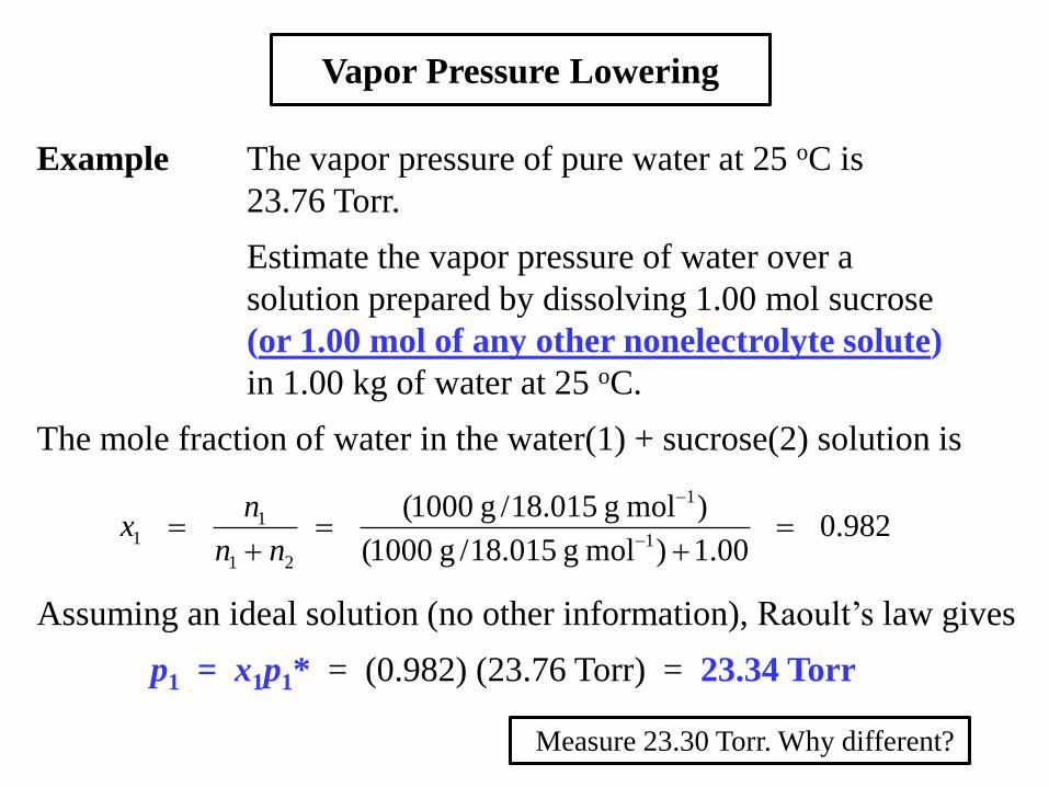
Example The vapor pressure of pure water at 25 oC is
23.76 Torr.
Estimate the vapor pressure of water over a
solution prepared by dissolving 1.00 mol sucrose
(or 1.00 mol of any other nonelectrolyte solute)
in 1.00 kg of water at 25 oC.
The mole fraction of water in the water(1) + sucrose(2) solution is
Vapor Pressure Lowering
982.000.1)mol g015.18/g1000(
)mol g015.18/g1000(1
1
21
11
nn
nx
Assuming an ideal solution (no other information), Raoult’s law gives
p1 = x1p1* = (0.982) (23.76 Torr) = 23.34 Torr
Measure 23.30 Torr. Why different?
Freezing Point Depression
Salt (NaCl) spread on winter roads melts ice. Why?
But if it gets really cold (< 15 oC), no melting. Why?
Can other compounds melt ice?
Thermodynamics of automotive antifreeze products?
F.p. depression is used to measure molecular weights. How?
Solid-liquid phase diagrams introduced
How does purification by re-crystallization work?
Section 9.7 Freezing Point Depression
and Boiling Point Elevation
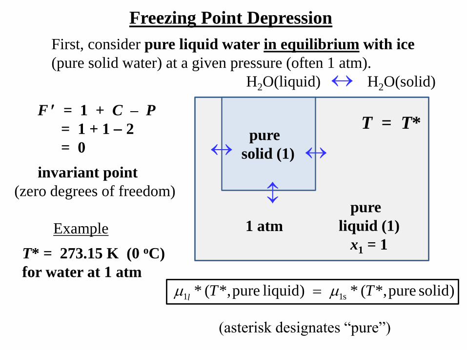
Freezing Point Depression
First, consider pure liquid water in equilibrium with ice
(pure solid water) at a given pressure (often 1 atm).
H2O(liquid) H2O(solid)
)solid pure*,(*)liquid pure*,(* s11 TTl
F = 1 + C – P
= 1 + 1 2
= 0
invariant point
(zero degrees of freedom)
Example
T* = 273.15 K (0 oC)
for water at 1 atm
pure
solid (1)
pure
liquid (1)
x1 = 1
(asterisk designates “pure”)
T = T*
1 atm
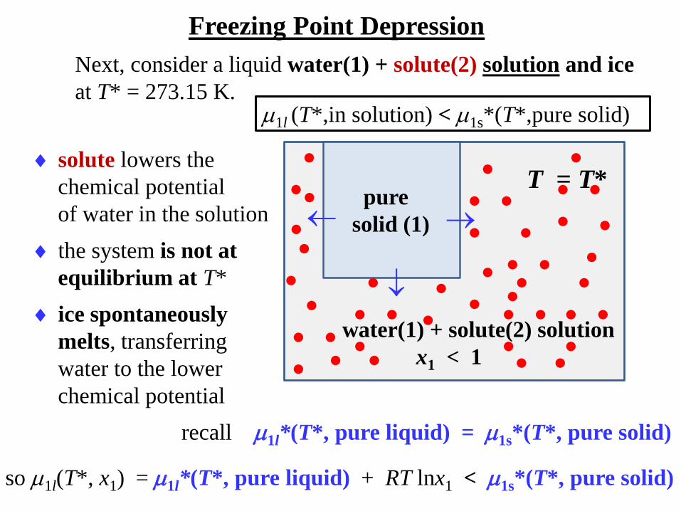
Freezing Point Depression
Next, consider a liquid water(1) + solute(2) solution and ice
at T* = 273.15 K.
pure
solid (1)
water(1) + solute(2) solution
x1 < 1
T = T*
solute lowers the
chemical potential
of water in the solution
the system is not at
equilibrium at T*
ice spontaneously
melts, transferring
water to the lower
chemical potential
recall 1l*(T*, pure liquid) = 1s*(T*, pure solid)
so 1l(T*, x1) = 1l*(T*, pure liquid) + RT lnx1 < 1s*(T*, pure solid)
1l (T*,in solution) < 1s*(T*,pure solid)
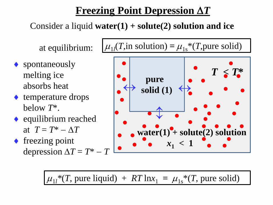
Freezing Point Depression T
Consider a liquid water(1) + solute(2) solution and ice
at equilibrium:
pure
solid (1)
water(1) + solute(2) solution
x1 < 1
T < T*
spontaneously
melting ice
absorbs heat
temperature drops
below T*.
equilibrium reached
at T = T* T
freezing point
depression T = T* T
1l*(T, pure liquid) + RT lnx1 = 1s*(T, pure solid)
1l(T,in solution) = 1s*(T,pure solid)
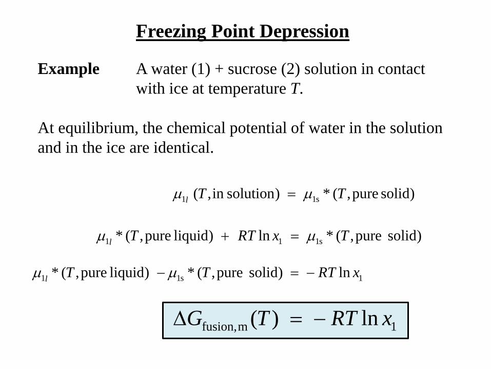
Freezing Point Depression
Example A water (1) + sucrose (2) solution in contact
with ice at temperature T.
At equilibrium, the chemical potential of water in the solution
and in the ice are identical.
)solid pure,(*)solutionin ,( s11 TTl
)solid pure,(*ln)liquid pure,(* s111 TxRTTl
1s11 ln)solid pure,(*)liquid pure,(* xRTTTl
1mfusion, ln)( xRTTG
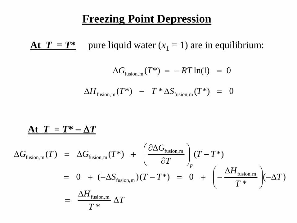
Freezing Point Depression
0)1ln(*)(mfusion, RTTG
At T = T* pure liquid water (x1 = 1) are in equilibrium:
0*)(**)( mfusion,mfusion, TSTTH
*)(*)()( mfusion,
mfusion,mfusion, TTT
GTGTG
p
)(*
0*)()(0 mfusion,
mfusion, TT
HTTS
At T = T* T
TT
H
*
mfusion,
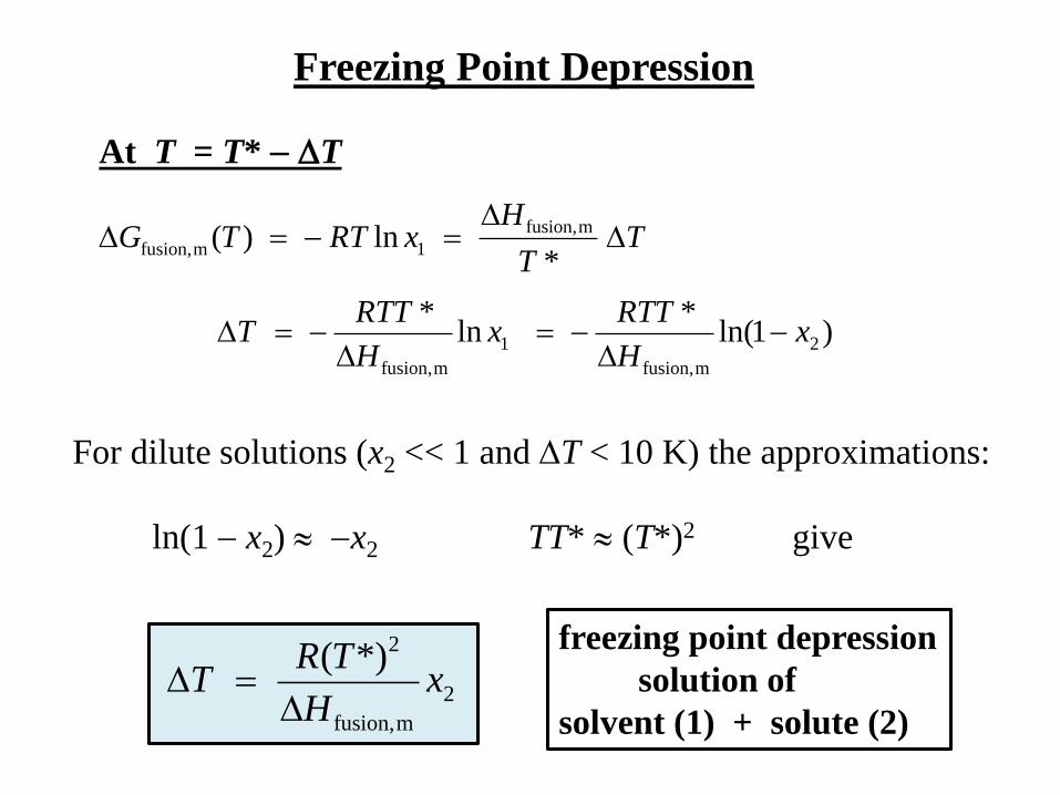
Freezing Point Depression
At T = T* T
TT
HxRTTG
*ln)( mfusion,
1mfusion,
)1ln(*
ln*
2
mfusion,
1
mfusion,
xH
RTTx
H
RTTT
For dilute solutions (x2 << 1 and T < 10 K) the approximations:
ln(1 x2) x2 TT* (T*)2 give
2
mfusion,
2*)(x
H
TRT
freezing point depression
solution of
solvent (1) + solute (2)
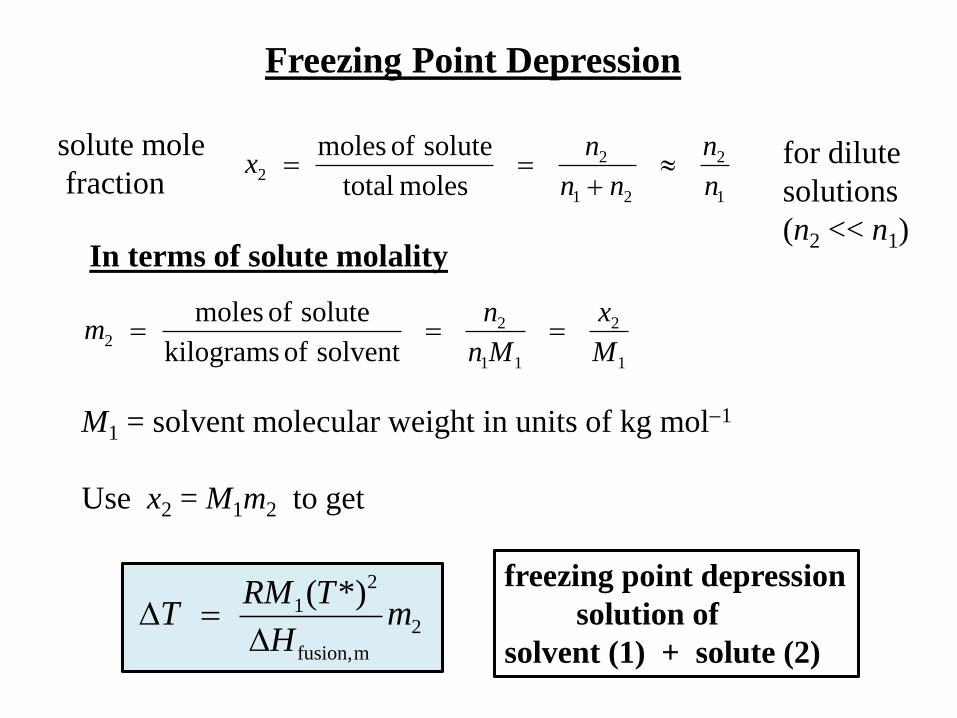
Freezing Point Depression
In terms of solute molality
1
2
11
22
solvent of kilograms
solute of moles
M
x
Mn
nm
2
mfusion,
2
1 *)(m
H
TRMT
freezing point depression
solution of
solvent (1) + solute (2)
solute mole
fraction 1
2
21
22
moles total
solute of moles
n
n
nn
nx
for dilute
solutions
(n2 << n1)
M1 = solvent molecular weight in units of kg mol1
Use x2 = M1m2 to get
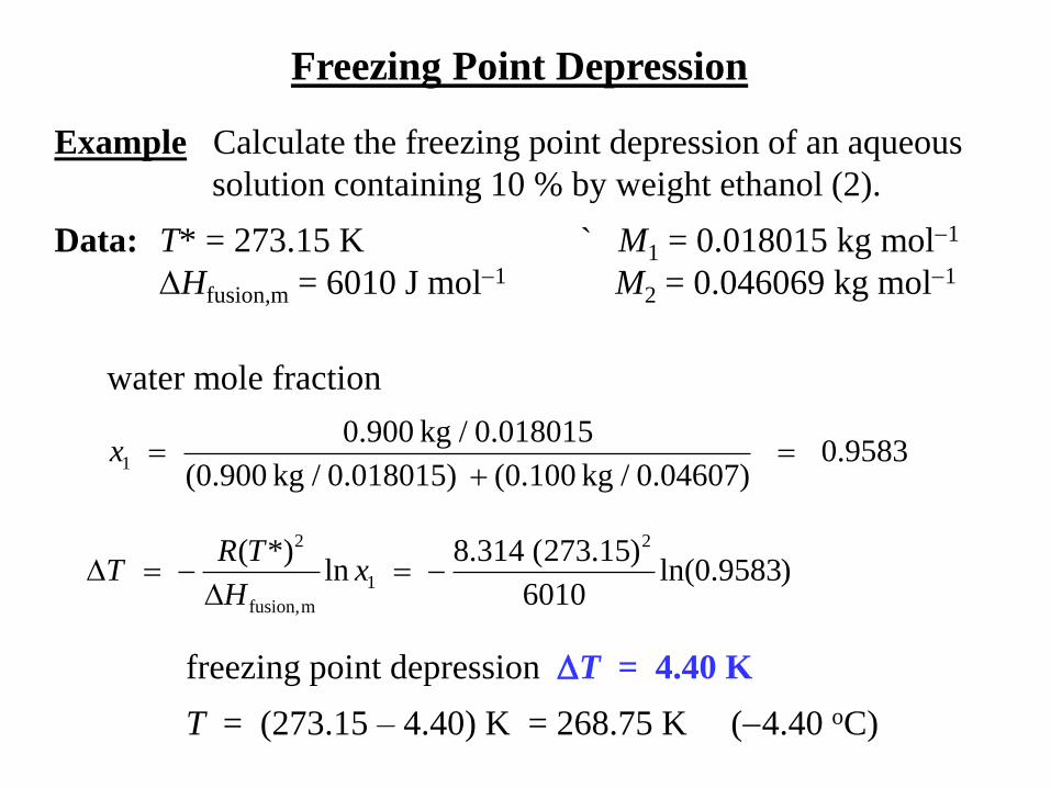
Freezing Point Depression
Example Calculate the freezing point depression of an aqueous
solution containing 10 % by weight ethanol (2).
Data: T* = 273.15 K ` M1 = 0.018015 kg mol1
Hfusion,m = 6010 J mol1 M2 = 0.046069 kg mol1
9583.00.04607) / kg (0.100 0.018015) / kg (0.900
0.018015 / kg 0.9001
x
)9583.0ln(6010
)15.273(314.8ln
*)( 2
1
mfusion,
2
xH
TRT
water mole fraction
freezing point depression T = 4.40 K
T = (273.15 – 4.40) K = 268.75 K (4.40 oC)
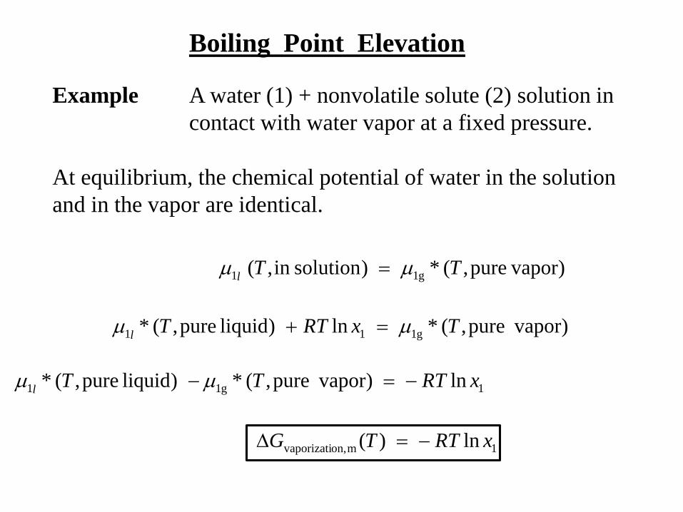
Boiling Point Elevation
Example A water (1) + nonvolatile solute (2) solution in
contact with water vapor at a fixed pressure.
At equilibrium, the chemical potential of water in the solution
and in the vapor are identical.
) vaporpure,(*)solutionin ,( g11 TTl
) vaporpure,(*ln)liquid pure,(* g111 TxRTTl
1g11 ln) vaporpure,(*)liquid pure,(* xRTTTl
1mon,vaporizati ln)( xRTTG
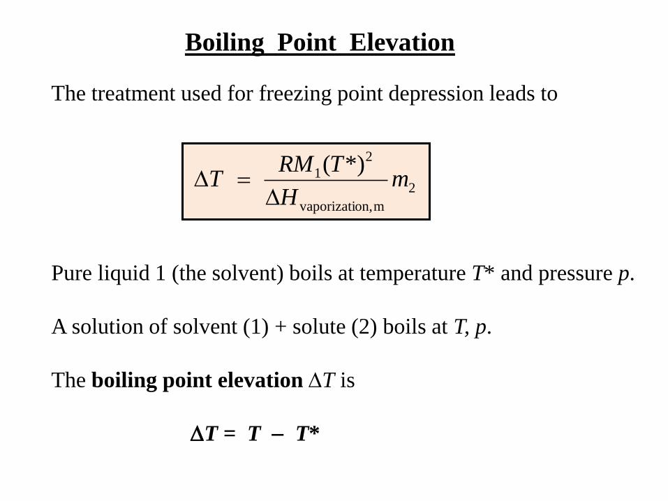
Boiling Point Elevation
The treatment used for freezing point depression leads to
2
mon,vaporizati
2
1 *)(m
H
TRMT
Pure liquid 1 (the solvent) boils at temperature T* and pressure p.
A solution of solvent (1) + solute (2) boils at T, p.
The boiling point elevation T is
T = T T*
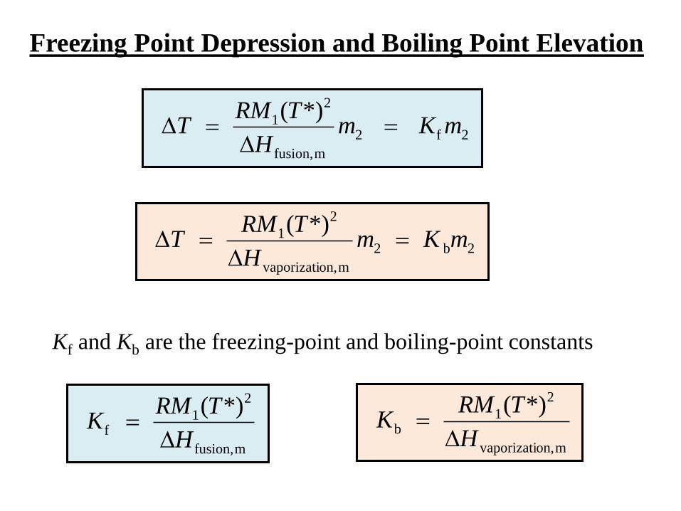
Freezing Point Depression and Boiling Point Elevation
2b2
mon,vaporizati
2
1 *)(mKm
H
TRMT
Kf and Kb are the freezing-point and boiling-point constants
2f2
mfusion,
2
1 *)(mKm
H
TRMT
mfusion,
2
1f
*)(
H
TRMK
mon,vaporizati
2
1b
*)(
H
TRMK
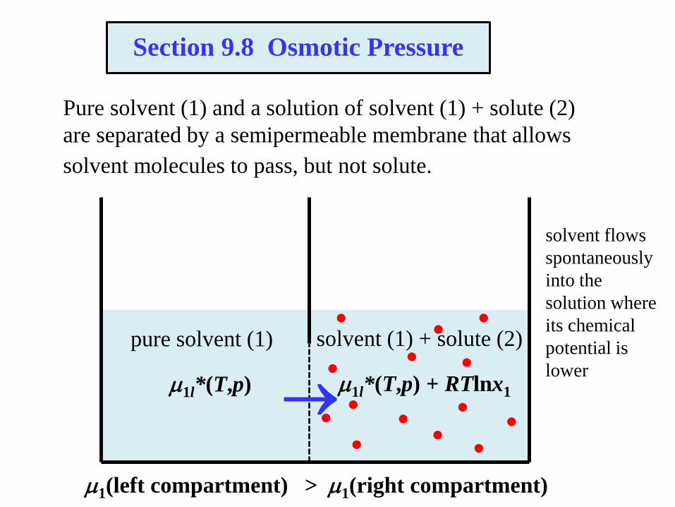
Pure solvent (1) and a solution of solvent (1) + solute (2)
are separated by a semipermeable membrane that allows
solvent molecules to pass, but not solute.
Section 9.8 Osmotic Pressure
pure solvent (1) solvent (1) + solute (2)
1l*(T,p) 1l*(T,p) + RTlnx1
1(left compartment) > 1(right compartment)
solvent flows
spontaneously
into the
solution where
its chemical
potential is
lower
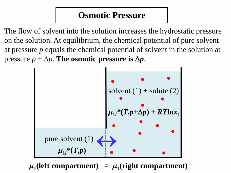
The flow of solvent into the solution increases the hydrostatic pressure
on the solution. At equilibrium, the chemical potential of pure solvent
at pressure p equals the chemical potential of solvent in the solution at
pressure p + p. The osmotic pressure is p.
Osmotic Pressure
pure solvent (1)
solvent (1) + solute (2)
1l*(T,p)
1l*(T,p+p) + RTlnx1
1(left compartment) = 1(right compartment)
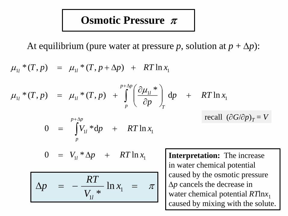
At equilibrium (pure water at pressure p, solution at p + p):
Osmotic Pressure
111 ln),(*),(* xRTppTpT ll
11
11 lnd*
),(*),(* xRTpp
pTpT
T
pp
p
lll
11 lnd*0 xRTpV
pp
p
l
11 ln*0 xRTpV l
1
1
ln*
xV
RTp
l
recall (G/p)T = V
Interpretation: The increase
in water chemical potential
caused by the osmotic pressure
p cancels the decrease in
water chemical potential RTlnx1
caused by mixing with the solute.
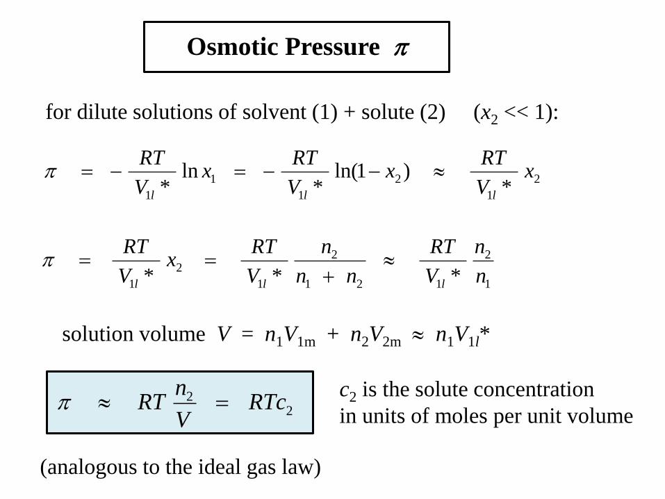
Osmotic Pressure
2
1
2
1
1
1 *)1ln(
*ln
*x
V
RTx
V
RTx
V
RT
lll
for dilute solutions of solvent (1) + solute (2) (x2 << 1):
1
2
121
2
1
2
1 *** n
n
V
RT
nn
n
V
RTx
V
RT
lll
solution volume V = n1V1m + n2V2m n1V1l*
22 RTc
V
nRT
c2 is the solute concentration
in units of moles per unit volume
(analogous to the ideal gas law)
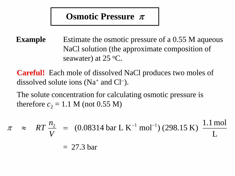
Osmotic Pressure
Example Estimate the osmotic pressure of a 0.55 M aqueous
NaCl solution (the approximate composition of
seawater) at 25 oC.
L
mol1.1)K15.298()molKLbar08314.0( 112
V
nRT
Careful! Each mole of dissolved NaCl produces two moles of
dissolved solute ions (Na+ and Cl).
The solute concentration for calculating osmotic pressure is
therefore c2 = 1.1 M (not 0.55 M)
= 27.3 bar
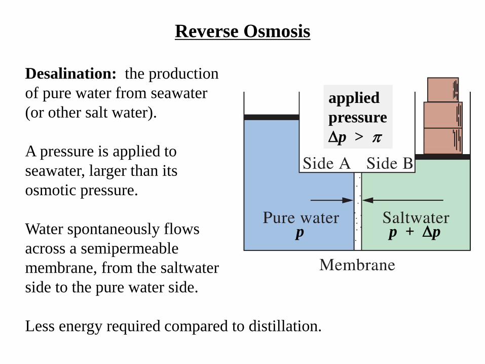
Reverse Osmosis
Desalination: the production
of pure water from seawater
(or other salt water).
A pressure is applied to
seawater, larger than its
osmotic pressure.
Water spontaneously flows
across a semipermeable
membrane, from the saltwater
side to the pure water side.
Less energy required compared to distillation.
p p + p
applied
pressure
p >
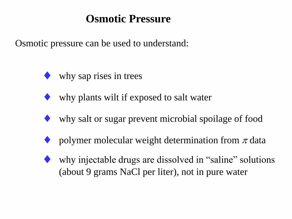
Osmotic Pressure
Osmotic pressure can be used to understand:
why sap rises in trees
why plants wilt if exposed to salt water
why salt or sugar prevent microbial spoilage of food
polymer molecular weight determination from data
why injectable drugs are dissolved in “saline” solutions
(about 9 grams NaCl per liter), not in pure water
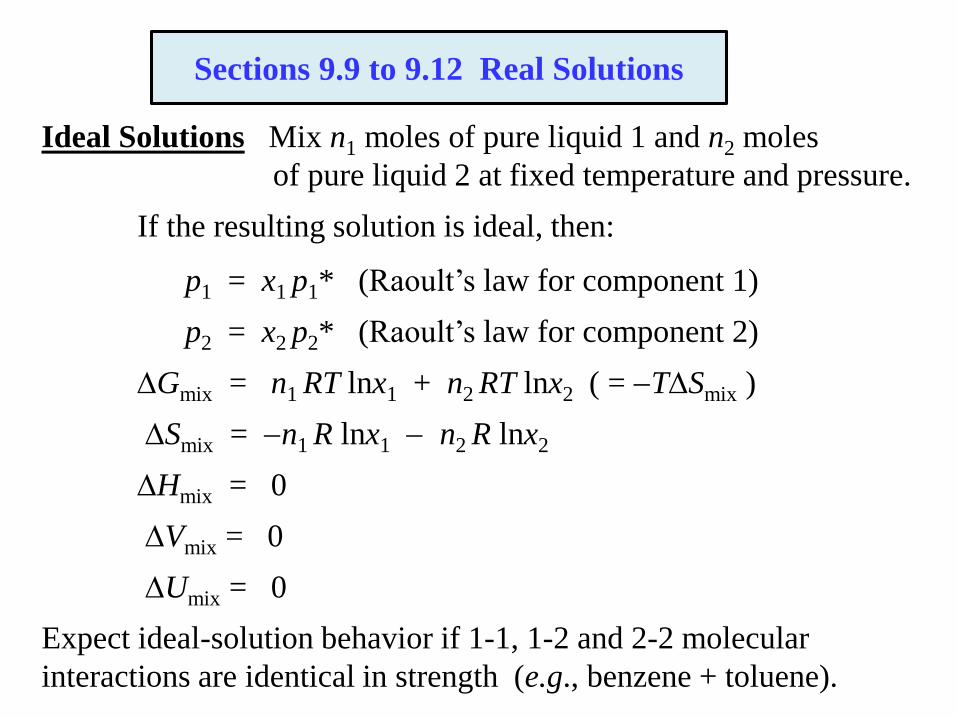
Ideal Solutions Mix n1 moles of pure liquid 1 and n2 moles
of pure liquid 2 at fixed temperature and pressure.
If the resulting solution is ideal, then:
p1 = x1 p1* (Raoult’s law for component 1)
p2 = x2 p2* (Raoult’s law for component 2)
Gmix = n1 RT lnx1 + n2 RT lnx2 ( = TSmix )
Smix = n1 R lnx1 n2 R lnx2
Hmix = 0
Vmix = 0
Umix = 0
Expect ideal-solution behavior if 1-1, 1-2 and 2-2 molecular
interactions are identical in strength (e.g., benzene + toluene).
Sections 9.9 to 9.12 Real Solutions
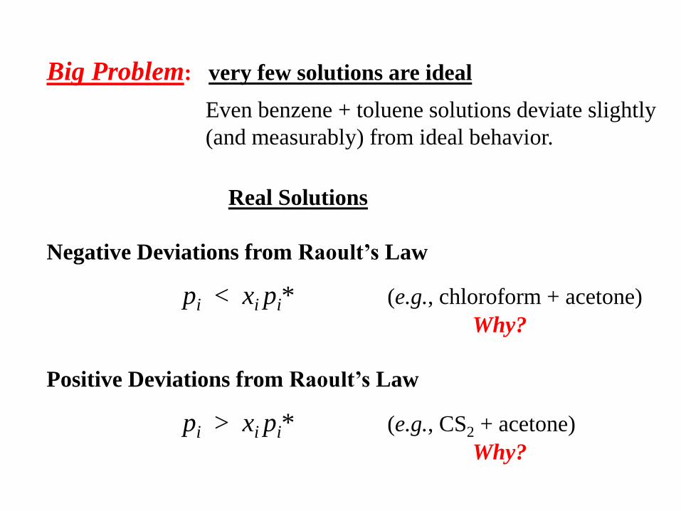
Big Problem: very few solutions are ideal
Even benzene + toluene solutions deviate slightly
(and measurably) from ideal behavior.
Real Solutions
Negative Deviations from Raoult’s Law
pi < xi pi* (e.g., chloroform + acetone)
Why?
Positive Deviations from Raoult’s Law
pi > xi pi* (e.g., CS2 + acetone)
Why?
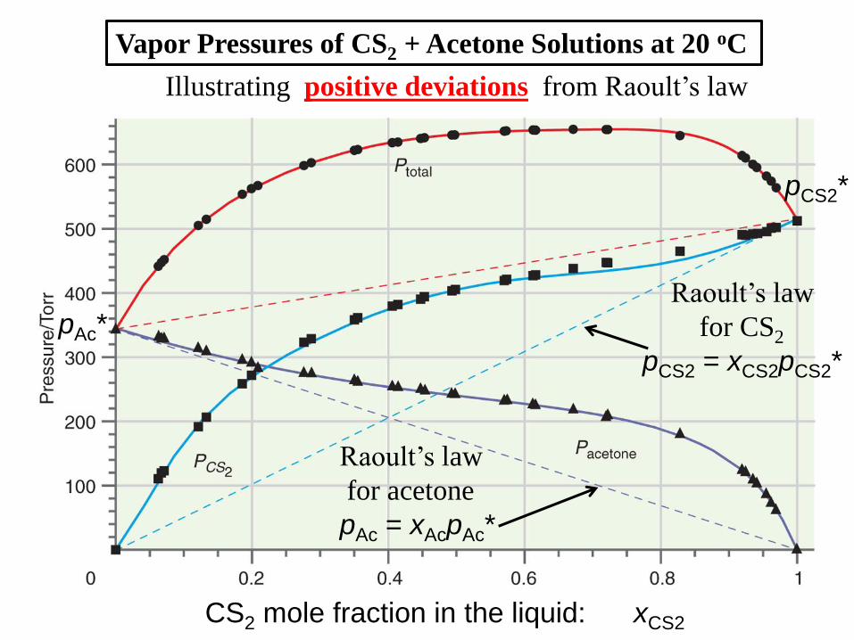
Vapor Pressures of CS2 + Acetone Solutions at 20 oC
Raoult’s law
for CS2
pCS2 = xCS2pCS2*
Raoult’s law
for acetone
pAc = xAcpAc*
Illustrating positive deviations from Raoult’s law
CS2 mole fraction in the liquid: xCS2
pCS2*
pAc*
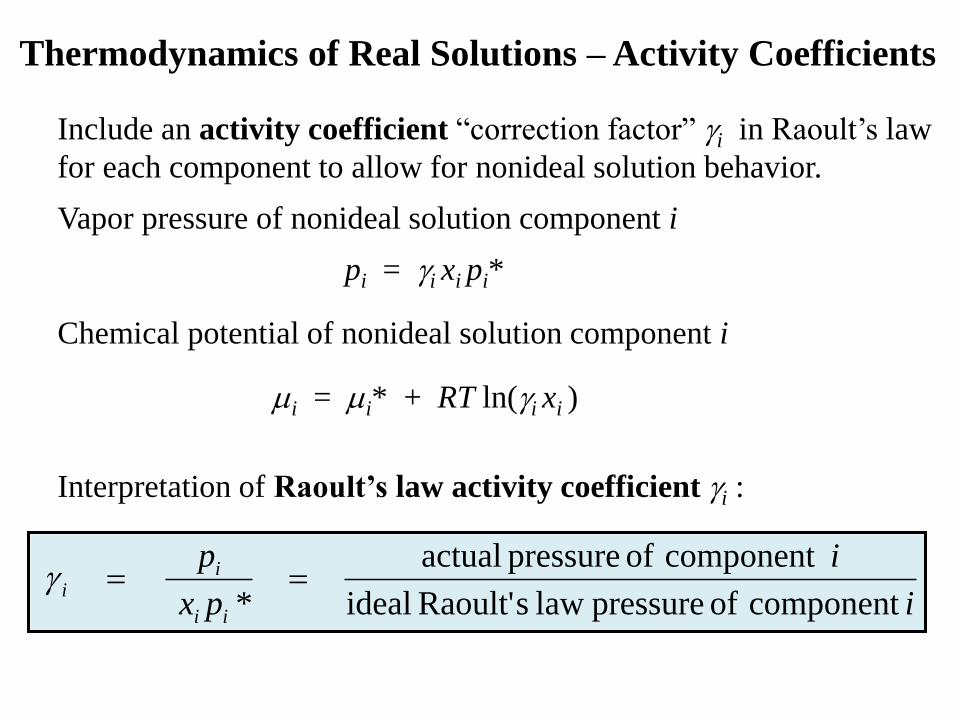
Thermodynamics of Real Solutions – Activity Coefficients
Include an activity coefficient “correction factor” i in Raoult’s law
for each component to allow for nonideal solution behavior.
Vapor pressure of nonideal solution component i
pi = i xi pi*
Chemical potential of nonideal solution component i
i = i* + RT ln(i xi )
Interpretation of Raoult’s law activity coefficient i :
i
i
px
p
ii
ii
component of pressure law sRaoult' ideal
component of pressure actual
*
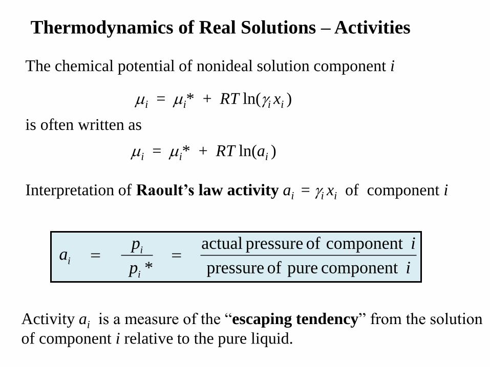
Thermodynamics of Real Solutions – Activities
The chemical potential of nonideal solution component i
i = i* + RT ln(i xi )
is often written as
i = i* + RT ln(ai )
Interpretation of Raoult’s law activity ai = i xi of component i
i
i
p
pa
i
ii
component pure of pressure
component of pressure actual
*
Activity ai is a measure of the “escaping tendency” from the solution
of component i relative to the pure liquid.
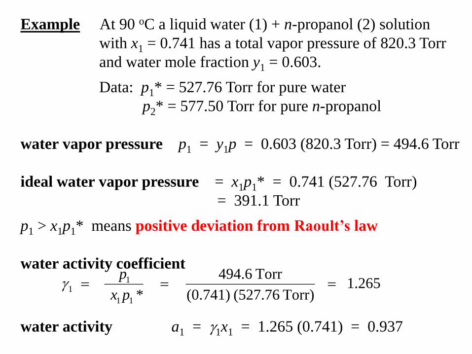
Example At 90 oC a liquid water (1) + n-propanol (2) solution
with x1 = 0.741 has a total vapor pressure of 820.3 Torr
and water mole fraction y1 = 0.603.
Data: p1* = 527.76 Torr for pure water
p2* = 577.50 Torr for pure n-propanol
water vapor pressure p1 = y1p = 0.603 (820.3 Torr) = 494.6 Torr
ideal water vapor pressure = x1p1* = 0.741 (527.76 Torr)
= 391.1 Torr
p1 > x1p1* means positive deviation from Raoult’s law
water activity coefficient
water activity a1 = 1x1 = 1.265 (0.741) = 0.937
265.1Torr)(527.76(0.741)
Torr494.6
*11
11
px
p
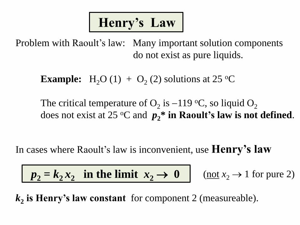
Henry’s Law
Problem with Raoult’s law: Many important solution components
do not exist as pure liquids.
Example: H2O (1) + O2 (2) solutions at 25 oC
The critical temperature of O2 is 119 oC, so liquid O2
does not exist at 25 oC and p2* in Raoult’s law is not defined.
In cases where Raoult’s law is inconvenient, use Henry’s law
(not x2 1 for pure 2)
k2 is Henry’s law constant for component 2 (measureable).
p2 = k2 x2 in the limit x2 0
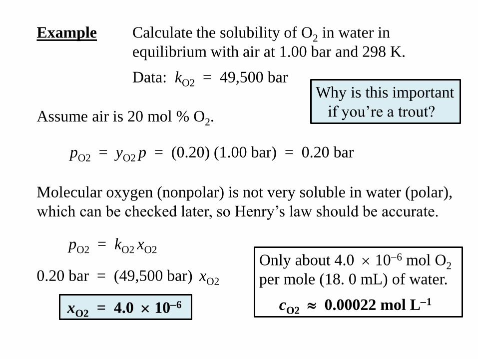
Example Calculate the solubility of O2 in water in
equilibrium with air at 1.00 bar and 298 K.
Data: kO2 = 49,500 bar
Assume air is 20 mol % O2.
pO2 = yO2 p = (0.20) (1.00 bar) = 0.20 bar
pO2 = kO2 xO2
Molecular oxygen (nonpolar) is not very soluble in water (polar),
which can be checked later, so Henry’s law should be accurate.
0.20 bar = (49,500 bar) xO2
xO2 = 4.0 106
Only about 4.0 106 mol O2
per mole (18. 0 mL) of water.
cO2 0.00022 mol L1
Why is this important
if you’re a trout?
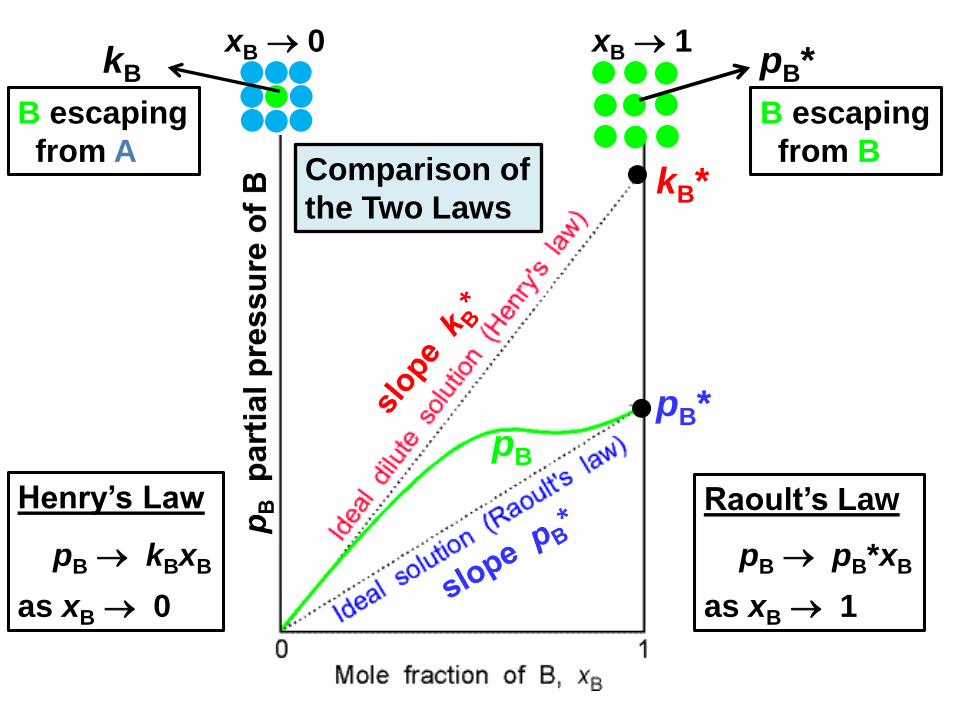
pB
pB*
kB*
pB*kB
Henry’s Law
pB kBxB
as xB 0
Raoult’s Law
pB pB*xB
as xB 1
B escaping
from A
B escaping
from B
xB 0 xB 1
Comparison of
the Two Laws
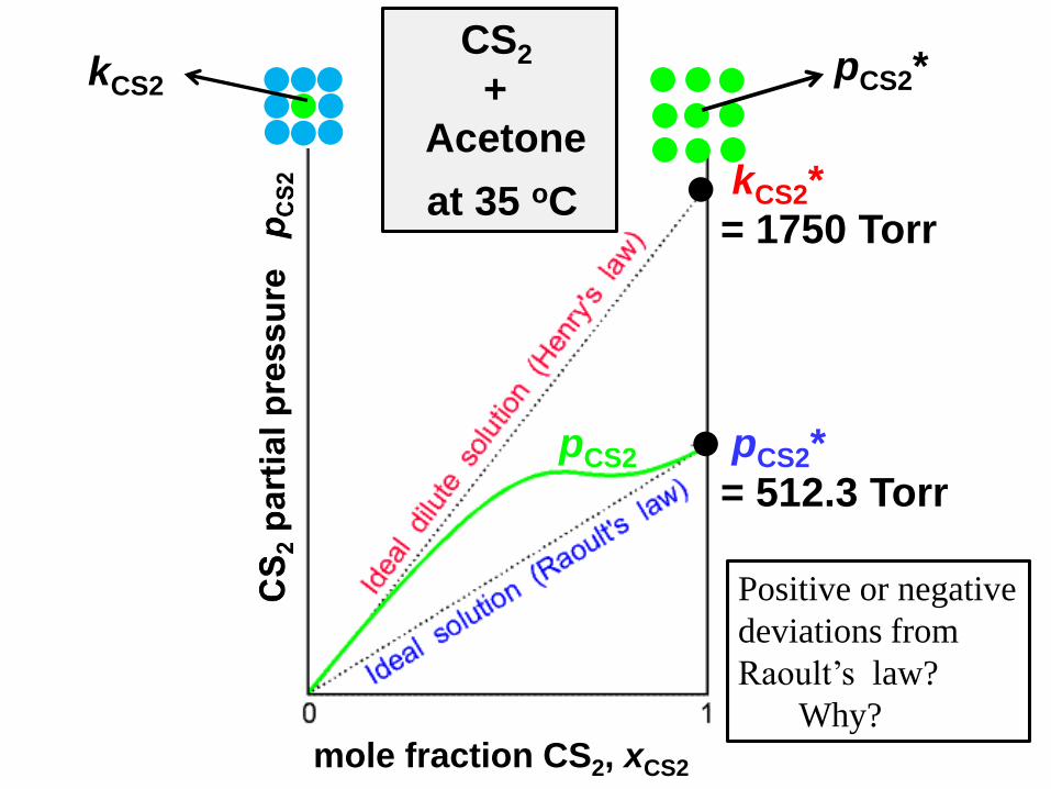
pCS2 pCS2*
= 512.3 Torr
kCS2*
= 1750 Torr
pCS2*kCS2
CS2
+
Acetone
at 35 oC
mole fraction CS2, xCS2
Positive or negative
deviations from
Raoult’s law?
Why?
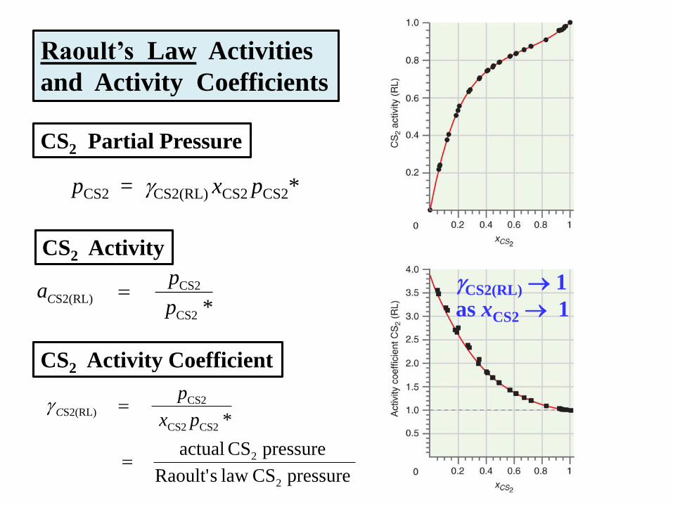
Raoult’s Law Activities
and Activity Coefficients
pCS2 = CS2(RL) xCS2 pCS2*
pressure CS law sRaoult'
pressure CS actual
*
2
2
CS2CS2
CS2S2(RL)
px
pC
CS2 Partial Pressure
CS2 Activity
*CS2
CS2S2(RL)
p
paC
CS2 Activity Coefficient
CS2(RL) 1
as xCS2 1
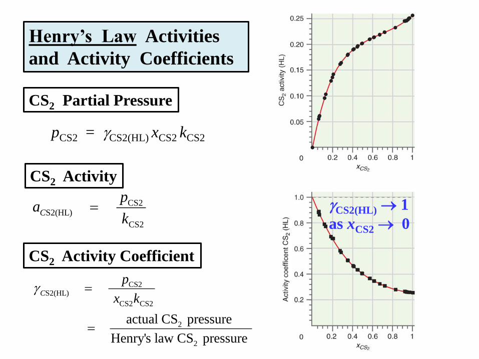
Henry’s Law Activities
and Activity Coefficients
pCS2 = CS2(HL) xCS2 kCS2
CS2S2(HL)
CS2 CS2
2
2
actual CS pressure
Henry's law CS pressure
C
p
x k
CS2 Partial Pressure
CS2 Activity
CS2S2(HL)
CS2
C
pa
k
CS2 Activity Coefficient
CS2(HL) 1
as xCS2 0
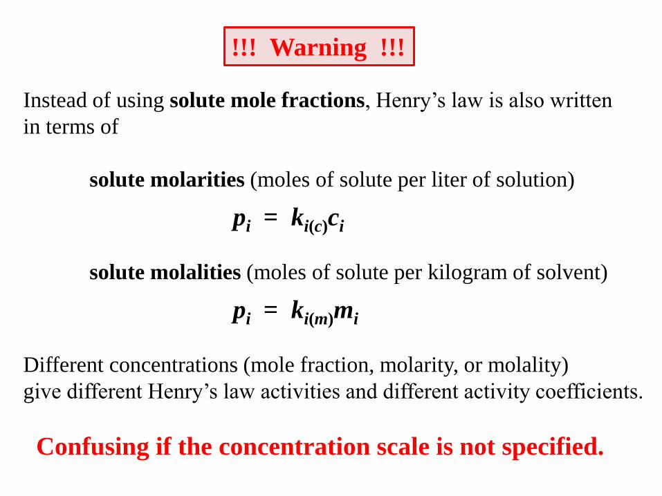
!!! Warning !!!
Instead of using solute mole fractions, Henry’s law is also written
in terms of
solute molarities (moles of solute per liter of solution)
pi = ki(c)ci
solute molalities (moles of solute per kilogram of solvent)
pi = ki(m)mi
Different concentrations (mole fraction, molarity, or molality)
give different Henry’s law activities and different activity coefficients.
Confusing if the concentration scale is not specified.
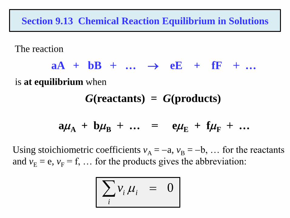
The reaction
aA + bB + … eE + fF + …
is at equilibrium when
G(reactants) = G(products)
aA + bB + … = eE + fF + …
Using stoichiometric coefficients vA = a, vB = b, … for the reactants
and vE = e, vF = f, … for the products gives the abbreviation:
Section 9.13 Chemical Reaction Equilibrium in Solutions
0i
iiv
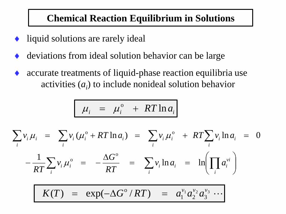
liquid solutions are rarely ideal
deviations from ideal solution behavior can be large
accurate treatments of liquid-phase reaction equilibria use
activities (ai) to include nonideal solution behavior
Chemical Reaction Equilibrium in Solutions
iii aRT lno
0ln)ln( oo i
ii
i
ii
i
iii
i
ii avRTvaRTvv
i
vi
i
i
ii
i
ii aavRT
Gv
RTlnln
1 oo
321
321
o )/exp()(vvv
aaaRTGTK
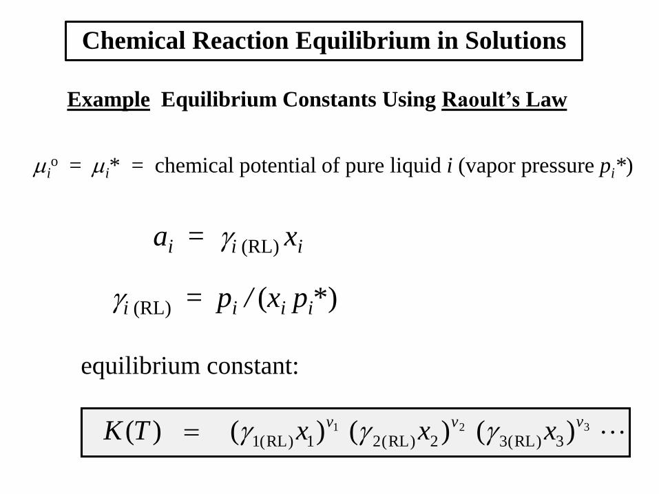
Example Equilibrium Constants Using Raoult’s Law
Chemical Reaction Equilibrium in Solutions
321 )()()()( 3)RL(32)RL(21)RL(1
vvvxxxTK
io = i* = chemical potential of pure liquid i (vapor pressure pi*)
ai = i (RL) xi
i (RL) = pi / (xi pi*)
equilibrium constant:
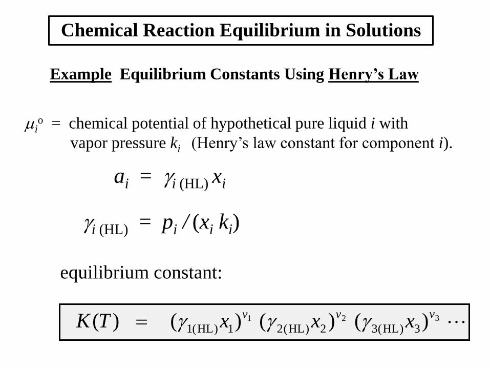
Example Equilibrium Constants Using Henry’s Law
Chemical Reaction Equilibrium in Solutions
321 )()()()( 3)HL(32)HL(21)HL(1
vvvxxxTK
io = chemical potential of hypothetical pure liquid i with
vapor pressure ki (Henry’s law constant for component i).
ai = i (HL) xi
i (HL) = pi / (xi ki)
equilibrium constant:
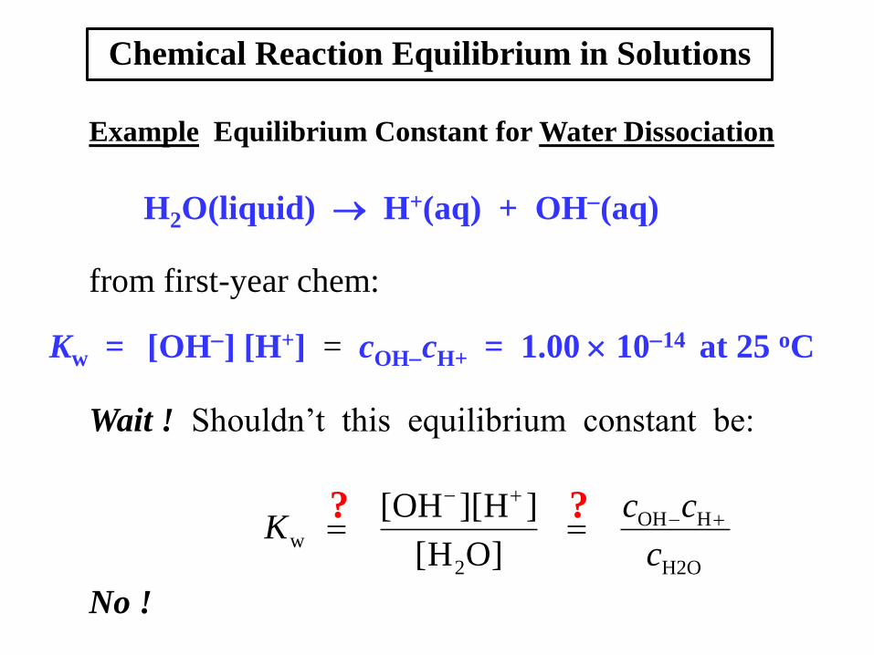
Example Equilibrium Constant for Water Dissociation
Chemical Reaction Equilibrium in Solutions
Wait ! Shouldn’t this equilibrium constant be:
No !
H2O(liquid) H+(aq) + OH(aq)
Kw = [OH] [H+] = cOHcH+ = 1.00 1014 at 25 oC
H2O
HOH
2
w]OH[
]H][OH[
c
ccK
??
from first-year chem:
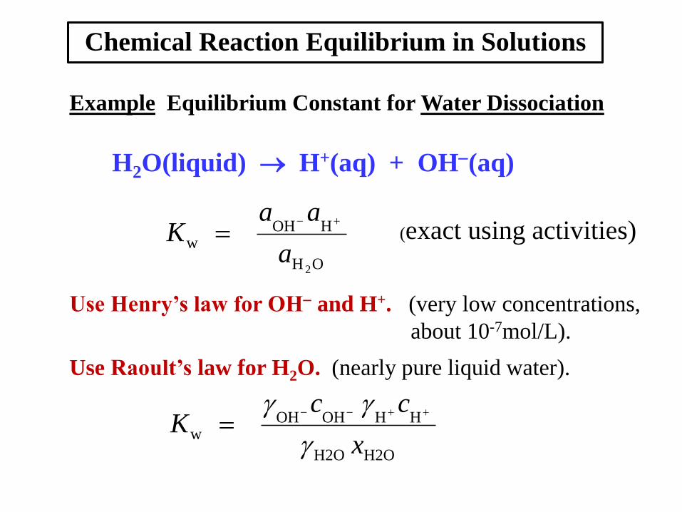
Example Equilibrium Constant for Water Dissociation
Chemical Reaction Equilibrium in Solutions
H2O(liquid) H+(aq) + OH(aq)
OH
HOHw
2a
aaK
(exact using activities)
H2OH2O
HHOHOHw
x
ccK
Use Henry’s law for OH and H+. (very low concentrations,
about 10-7mol/L).
Use Raoult’s law for H2O. (nearly pure liquid water).
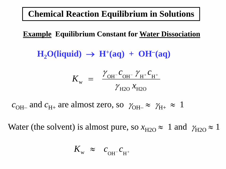
Example Equilibrium Constant for Water Dissociation
Chemical Reaction Equilibrium in Solutions
H2O(liquid) H+(aq) + OH(aq)
cOH and cH+ are almost zero, so OH H+ 1
H2OH2O
HHOHOHw
x
ccK
Water (the solvent) is almost pure, so xH2O 1 and H2O 1
HOHw ccK
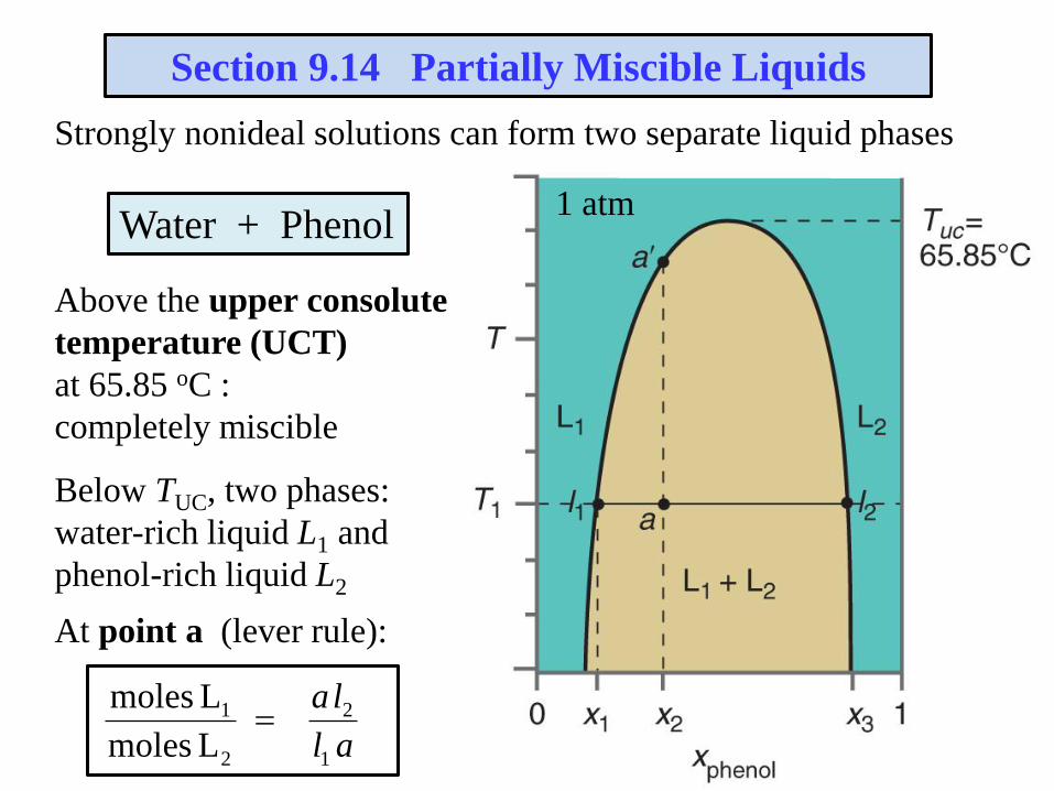
Strongly nonideal solutions can form two separate liquid phases
Section 9.14 Partially Miscible Liquids
Water + Phenol
Above the upper consolute
temperature (UCT)
at 65.85 oC :
completely miscible
Below TUC, two phases:
water-rich liquid L1 and
phenol-rich liquid L2
At point a (lever rule):
1 atm
al
la
1
2
2
1
L moles
L moles
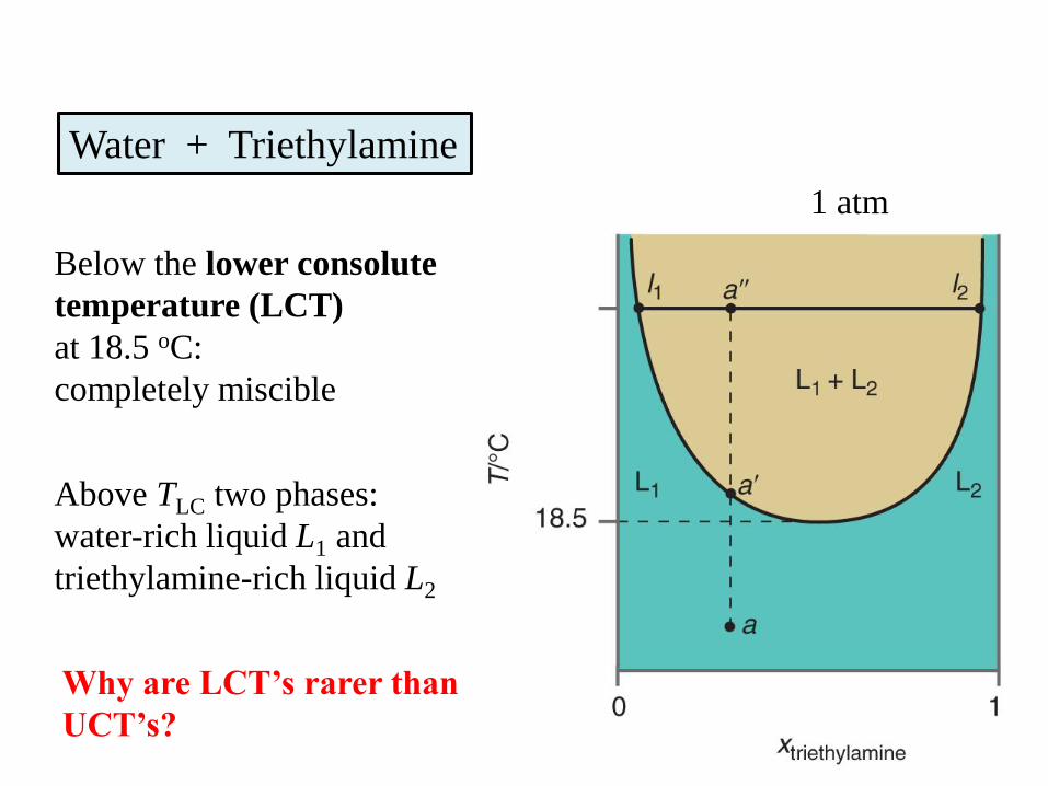
Water + Triethylamine
Below the lower consolute
temperature (LCT)
at 18.5 oC:
completely miscible
Above TLC two phases:
water-rich liquid L1 and
triethylamine-rich liquid L2
1 atm
Why are LCT’s rarer than
UCT’s?
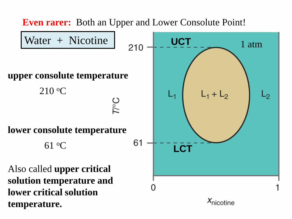
Water + Nicotine
upper consolute temperature
210 oC
lower consolute temperature
61 oC
Also called upper critical
solution temperature and
lower critical solution
temperature.
1 atm
Even rarer: Both an Upper and Lower Consolute Point!
UCT
LCT
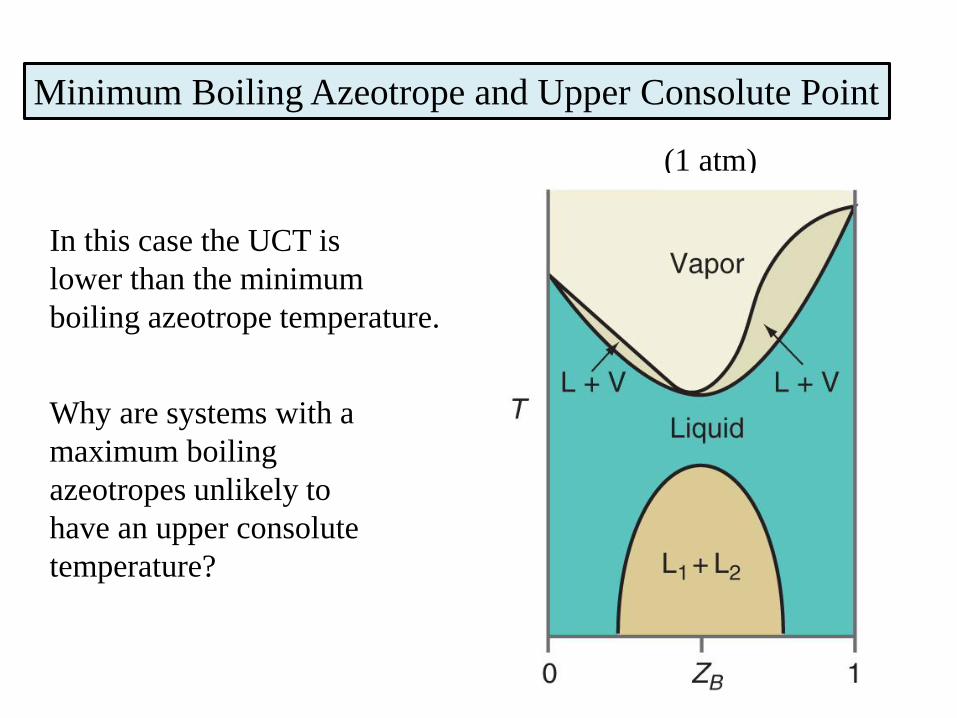
Minimum Boiling Azeotrope and Upper Consolute Point
In this case the UCT is
lower than the minimum
boiling azeotrope temperature.
Why are systems with a
maximum boiling
azeotropes unlikely to
have an upper consolute
temperature?
(1 atm)
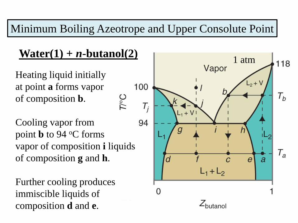
Minimum Boiling Azeotrope and Upper Consolute Point
Heating liquid initially
at point a forms vapor
of composition b.
Cooling vapor from
point b to 94 oC forms
vapor of composition i liquids
of composition g and h.
Further cooling produces
immiscible liquids of
composition d and e.
1 atmWater(1) + n-butanol(2)
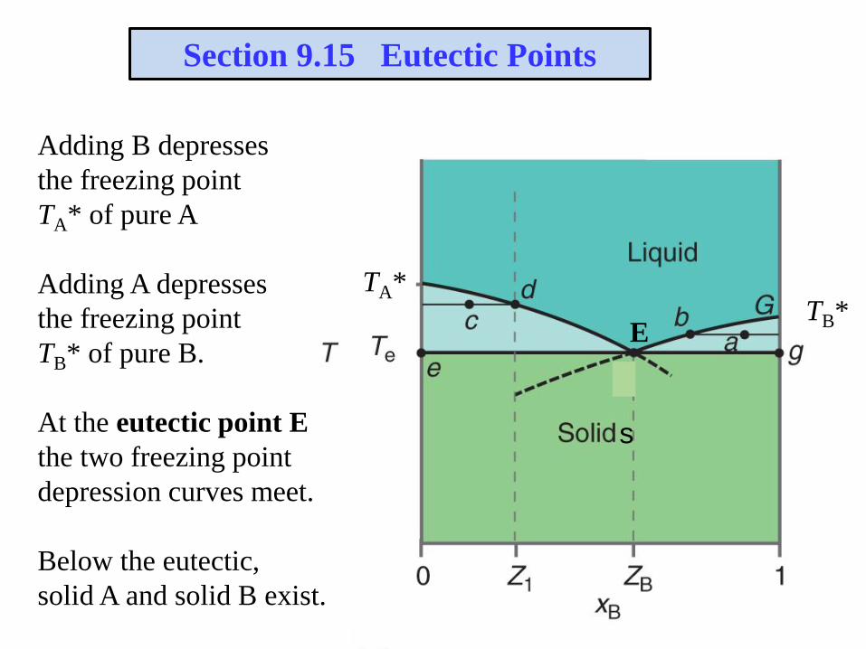
Section 9.15 Eutectic Points
Adding B depresses
the freezing point
TA* of pure A
Adding A depresses
the freezing point
TB* of pure B.
At the eutectic point E
the two freezing point
depression curves meet.
Below the eutectic,
solid A and solid B exist.
TA*TB*
E
s
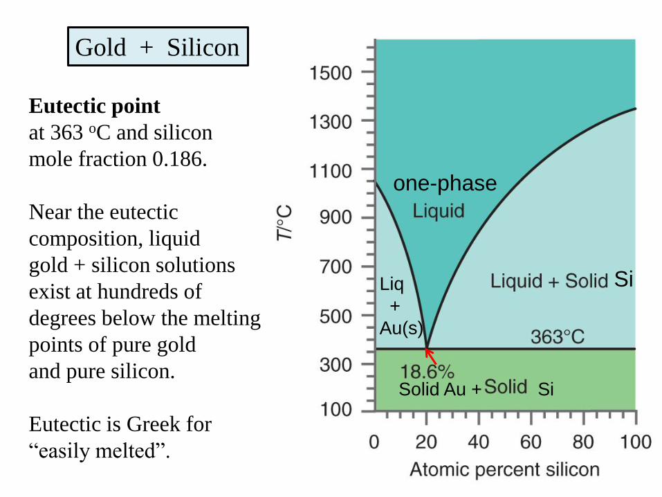
Gold + Silicon
Eutectic point
at 363 oC and silicon
mole fraction 0.186.
Near the eutectic
composition, liquid
gold + silicon solutions
exist at hundreds of
degrees below the melting
points of pure gold
and pure silicon.
Eutectic is Greek for
“easily melted”.
1 atm
one-phase
SiLiq
+
Au(s)
Solid Au + Si
xA
0.0 0.2 0.4 0.6 0.8 1.0
t /
oC
-20
0
20
40
60
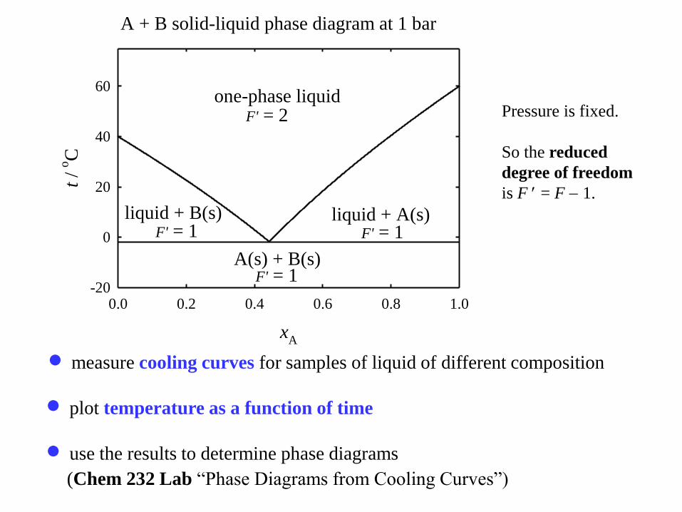
A + B solid-liquid phase diagram at 1 bar
one-phase liquid
liquid + A(s)liquid + B(s)
A(s) + B(s)
F' = 2
F' = 1F' = 1
F' = 1
measure cooling curves for samples of liquid of different composition
plot temperature as a function of time
use the results to determine phase diagrams
(Chem 232 Lab “Phase Diagrams from Cooling Curves”)
Pressure is fixed.
So the reduced
degree of freedom
is F = F 1.
xA
0.0 0.2 0.4 0.6 0.8 1.0
t /
oC
-20
0
20
40
60
B(l)
B(s)
B(l)+B(s)
F = 0
C = 1
F = 0
C = 1
1
3
2 4
5
A(l)
A(s)
A(l)+A(s)
l (mixture) l (mixture) l (mixture)
l + B(s)
l + B(s) + A(s) l + B(s) + A(s) l + A(s) + B(s)
l + A(s)
B(s) + A(s) B(s) + A(s)
A(s)
+
B(s)
b
a
ta
d
e e e
c
tb
td
te tete
tct / oC
time
F = 0
C = 2F = 0
C = 2
F = 0
C = 2
xA
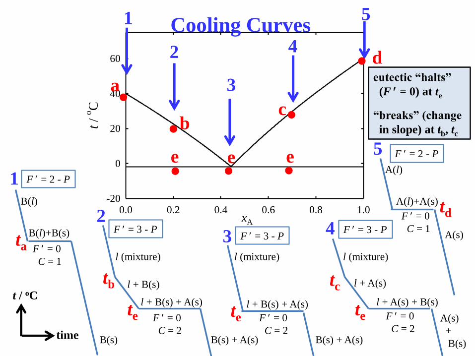
Cooling Curves
eutectic “halts”
(F = 0) at te
“breaks” (change
in slope) at tb, tc
1
23 4
5
F = 2 - P
F = 2 - P
F = 3 - PF = 3 - P
F = 3 - P
Chapter 10. Electrolyte Solutions
Summary
A whole chapter on just one kind of solution ?
What’s so special about electrolyte solutions ?
Enthalpy, entropy, and Gibbs energy of ions in solutions
Ion solvation
Activities of ions in solution
Debye-Huckel theory for dilute electrolyte solutions
Ionic reaction equilibrium
What is an “electrolyte solution” ?
a solution of ionic species of positive and negative
electrical charge dissolved in a solvent
the ions are mobile and conduct electric current in an
applied electric field (ionic conductivity)
usually ( but not always ) liquid solutions
important examples:
all biological and physiological solutions
strong acids and strong bases
buffer solutions for pH control
seawater, brines, and groundwater
battery electrolytes
molten salts
What’s Special About Electrolyte Solutions ?
thermodynamic properties of nonelectrolyte solution
components are functions of T, p, and composition
the properties of ions also depend on the electric potential
applied electric potential changes the chemical potential
of an ion of charge z by
electrical = zF
Example A 1.5 volt applied electric potential (from a common
AA battery) increases the chemical potential of Na+ ions by
electrical = zF = (+1) (96,485 C mol1) (1.5 V)
= 145,000 J mol1 (significant!!!)
application: electrochemical synthesis of sodium metal
Section 10.1 Enthalpy, Entropy, and Gibbs Energy
of Ions in Solution
electrolyte solutions are electrically neutral
impossible to study solutions containing only cations or anions
impossible to independently vary cation and anion concentrations
example aqueous MgCl2 solutions
2cMg2+ = cCl
important result: the internal energy, enthalpy, entropy, Gibbs
energy, volume, … of individual ions cannot be measured
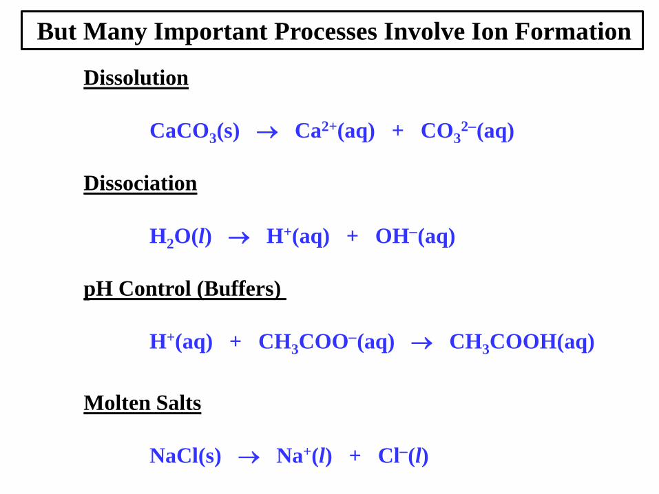
But Many Important Processes Involve Ion Formation
Dissolution
CaCO3(s) Ca2+(aq) + CO32(aq)
Dissociation
H2O(l) H+(aq) + OH(aq)
pH Control (Buffers)
H+(aq) + CH3COO(aq) CH3COOH(aq)
Molten Salts
NaCl(s) Na+(l) + Cl(l)
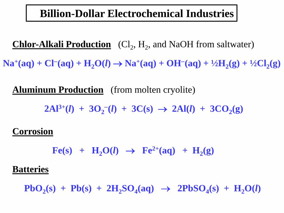
Billion-Dollar Electrochemical Industries
Chlor-Alkali Production (Cl2, H2, and NaOH from saltwater)
Na+(aq) + Cl(aq) + H2O(l) Na+(aq) + OH(aq) + ½H2(g) + ½Cl2(g)
Aluminum Production (from molten cryolite)
2Al3+(l) + 3O2(l) + 3C(s) 2Al(l) + 3CO2(g)
Corrosion
Fe(s) + H2O(l) Fe2+(aq) + H2(g)
Batteries
PbO2(s) + Pb(s) + 2H2SO4(aq) 2PbSO4(s) + H2O(l)
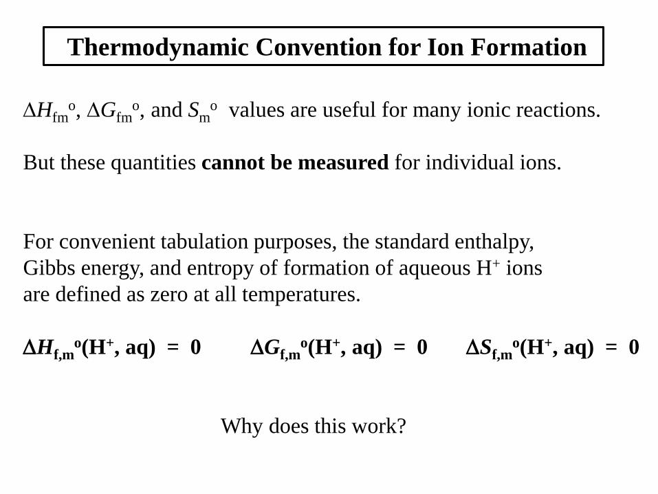
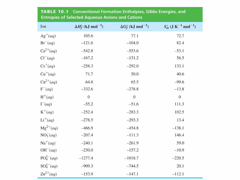
Thermodynamic Convention for Ion Formation
Hfmo, Gfm
o, and Smo values are useful for many ionic reactions.
But these quantities cannot be measured for individual ions.
For convenient tabulation purposes, the standard enthalpy,
Gibbs energy, and entropy of formation of aqueous H+ ions
are defined as zero at all temperatures.
Hf,mo(H+, aq) = 0 Gf,m
o(H+, aq) = 0 Sf,mo(H+, aq) = 0
Why does this work?
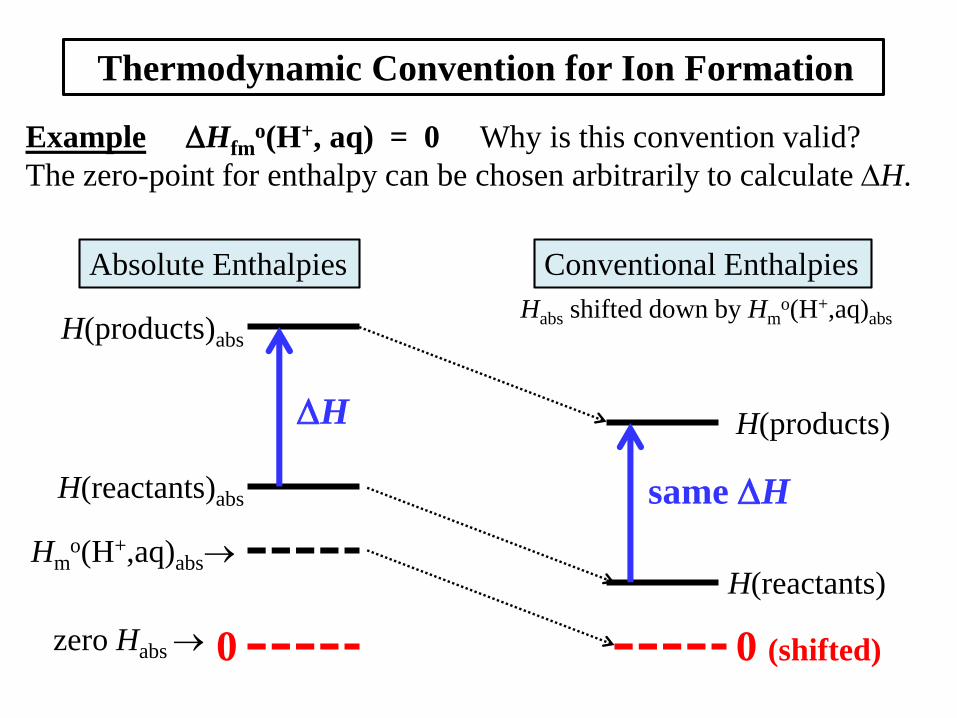
Thermodynamic Convention for Ion Formation
Example Hfmo(H+, aq) = 0 Why is this convention valid?
The zero-point for enthalpy can be chosen arbitrarily to calculate H.
H(products)abs
H(reactants)abs
zero Habs
Hmo(H+,aq)abs
Habs shifted down by Hmo(H+,aq)abs
H(products)
H(reactants)
0 0 (shifted)
Absolute Enthalpies Conventional Enthalpies
H
same H
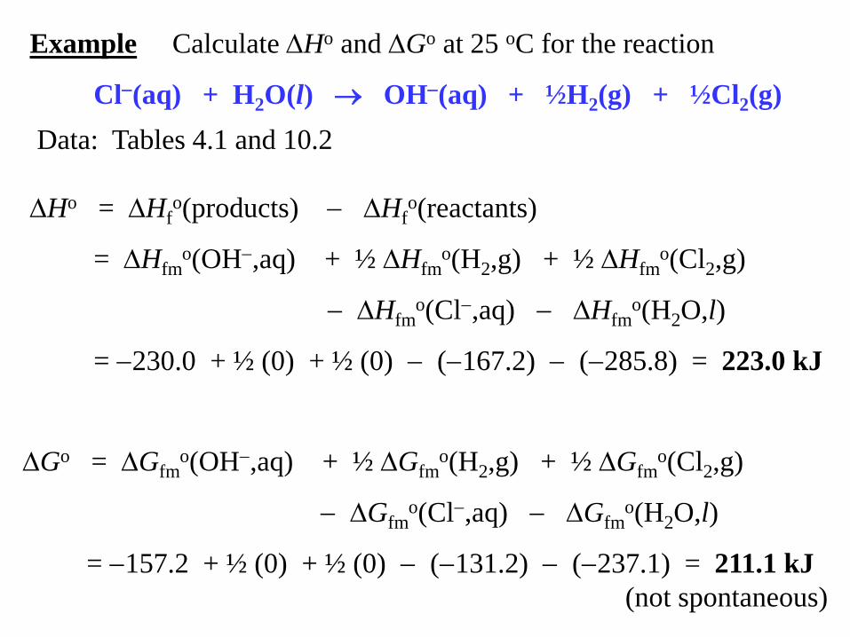
Example Calculate Ho and Go at 25 oC for the reaction
Cl(aq) + H2O(l) OH(aq) + ½H2(g) + ½Cl2(g)
Data: Tables 4.1 and 10.2
Ho = Hfo(products) Hf
o(reactants)
= Hfmo(OH,aq) + ½ Hfm
o(H2,g) + ½ Hfmo(Cl2,g)
Hfmo(Cl,aq) Hfm
o(H2O,l)
= 230.0 + ½ (0) + ½ (0) (167.2) (285.8) = 223.0 kJ
Go = Gfmo(OH,aq) + ½ Gfm
o(H2,g) + ½ Gfmo(Cl2,g)
Gfmo(Cl,aq) Gfm
o(H2O,l)
= 157.2 + ½ (0) + ½ (0) (131.2) (237.1) = 211.1 kJ
(not spontaneous)
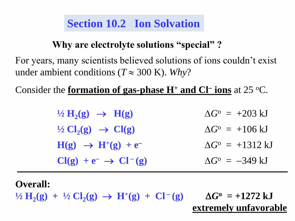
Section 10.2 Ion Solvation
Why are electrolyte solutions “special” ?
For years, many scientists believed solutions of ions couldn’t exist
under ambient conditions (T 300 K). Why?
Consider the formation of gas-phase H+ and Cl ions at 25 oC.
½ H2(g) H(g) Go = +203 kJ
½ Cl2(g) Cl(g) Go = +106 kJ
H(g) H+(g) + e Go = +1312 kJ
Cl(g) + e Cl (g) Go = 349 kJ
Overall:
½ H2(g) + ½ Cl2(g) H+(g) + Cl (g) Go = +1272 kJ
extremely unfavorable
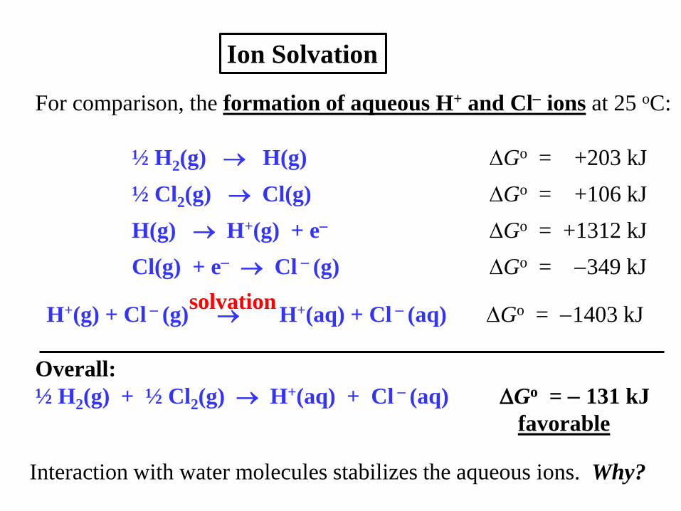
Ion Solvation
For comparison, the formation of aqueous H+ and Cl ions at 25 oC:
½ H2(g) H(g) Go = +203 kJ
½ Cl2(g) Cl(g) Go = +106 kJ
H(g) H+(g) + e Go = +1312 kJ
Cl(g) + e Cl (g) Go = 349 kJ
H+(g) + Cl (g) H+(aq) + Cl (aq) Go = 1403 kJ
Overall:
½ H2(g) + ½ Cl2(g) H+(aq) + Cl (aq) Go = 131 kJ
favorable
solvation
Interaction with water molecules stabilizes the aqueous ions. Why?
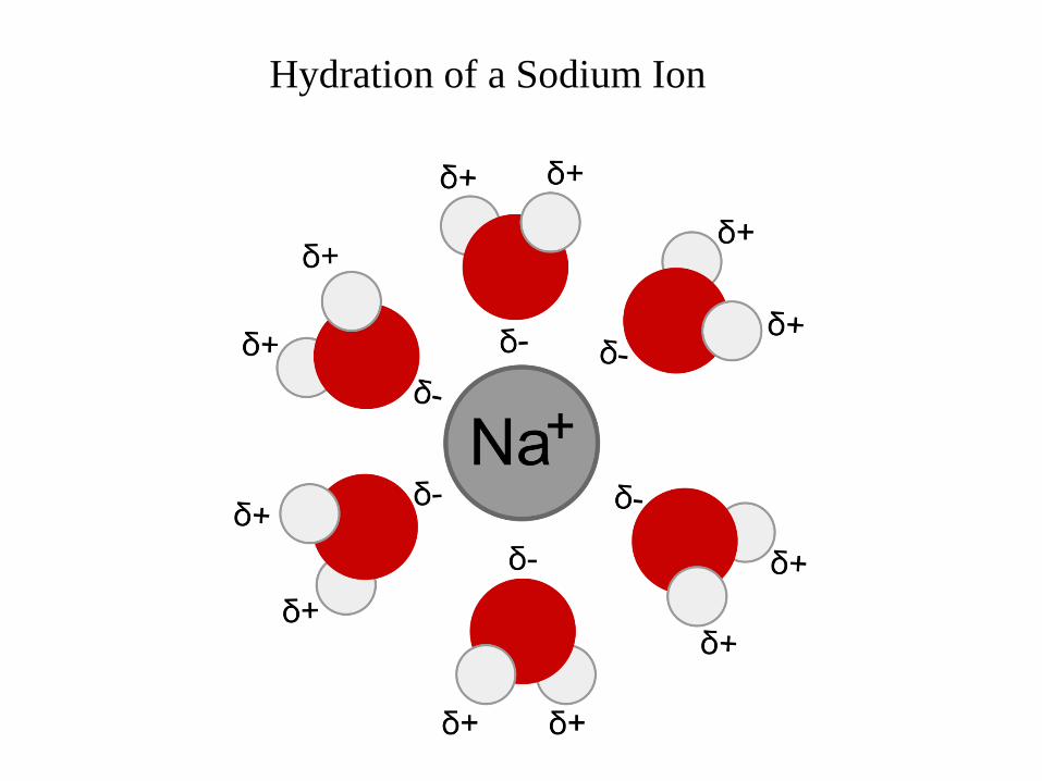
Hydration of a Sodium Ion
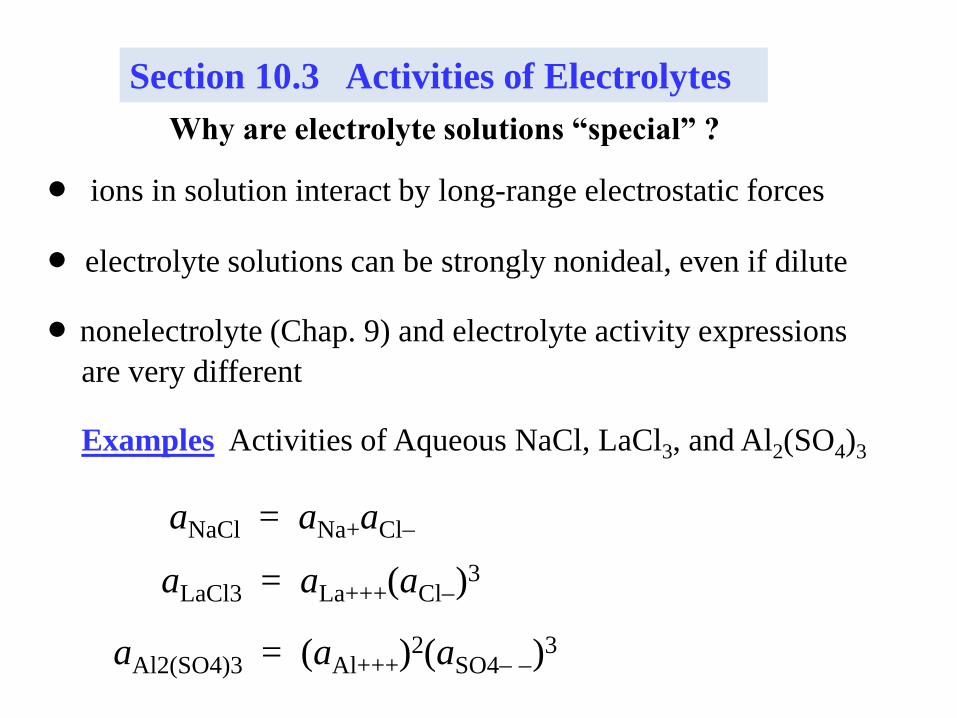
Section 10.3 Activities of Electrolytes
Why are electrolyte solutions “special” ?
ions in solution interact by long-range electrostatic forces
electrolyte solutions can be strongly nonideal, even if dilute
nonelectrolyte (Chap. 9) and electrolyte activity expressions
are very different
aNaCl = aNa+aCl
aLaCl3 = aLa+++(aCl)3
aAl2(SO4)3 = (aAl+++)2(aSO4 )3
Examples Activities of Aqueous NaCl, LaCl3, and Al2(SO4)3
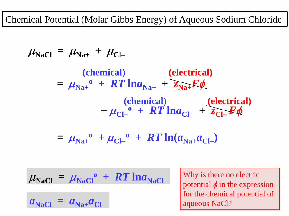
NaCl = Na+ + Cl
= Na+o + RT lnaNa+ + zNa+F
+ Clo + RT lnaCl + zCl F
= Na+o + Cl
o + RT ln(aNa+aCl)
NaCl = NaClo + RT lnaNaCl
aNaCl = aNa+aCl
Chemical Potential (Molar Gibbs Energy) of Aqueous Sodium Chloride
(chemical) (electrical)
(chemical) (electrical)
Why is there no electric
potential in the expression
for the chemical potential of
aqueous NaCl?
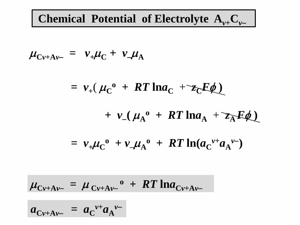
Cv+Av = v+C + vA
= v+( Co + RT lnaC + zCF )
+ v( Ao + RT lnaA + zA F )
= v+Co + vA
o + RT ln(aCv+aA
v)
Cv+Av = Cv+Avo + RT lnaCv+Av
aCv+Av = aCv+aA
v
Chemical Potential of Electrolyte Av+Cv
Cv+Av = Co + A
o + RT ln(aCv+aA
v)
a = (aCv+aA
v)1/v
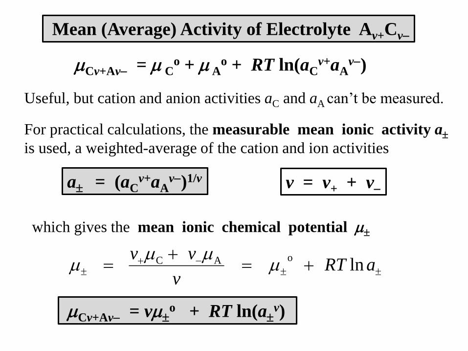
Mean (Average) Activity of Electrolyte Av+Cv
Useful, but cation and anion activities aC and aA can’t be measured.
For practical calculations, the measurable mean ionic activity ais used, a weighted-average of the cation and ion activities
which gives the mean ionic chemical potential
aRTv
vvln
oAC
v = v+ + v
Cv+Av = vo + RT ln(a
v)