chemistry 464 - people 464 manual.pdf · chemistry 464 . advanced physical . ... the physical...
TRANSCRIPT

CHEMISTRY 464
ADVANCED PHYSICAL CHEMISTRY LABORATORY
LABORATORY MANUAL
© P. S. Phillips 2010. All rights reserved.

Plot the graph, then put the data on.
There are no truths, only facts to be manipulated.
Give me six variables and I’ll fit an elephant. Give me seven and I’ll make it’s tail wag.

INSTRUCTIONS AND GENERAL INFORMATION. The physical chemistry laboratory is equipped for the following experiments. Students will carry out six of them. Each takes two lab sessions. Which experiments, and when you do them, will be organized the start of term. The experiments are done with partners.
These experiments are suites. Each suite consists of two or three experiments.
ID TOPIC EXPERIMENT
A Activity coefficients Activities of ions by electrochemistry (and some programming )*
E Enzyme kinetics Various approaches. Inhibition. Non-linear fitting.
G Thermodynamics of glycine Properties of a weak acid, pKa and thermochemistry.
H The hydrophobic effect A study of partitioning and co-solvents to illustrate the hydrophobic effect.
K Kinetics A couple of kinetics experiments, mainly to illustrate computer fitting methods.
M Micelles CMC and aggregation numbers by fluorimetry, UV-Vis and conductometry .
P Permeability A simple investigation of permeability and osmosis.
T Transitions in biomolecules Examine the effect of phase temperature and pH on myoglobin. Comparisons with other enzymes.
W Acidity of wines Look at the pH of mixed diprotic acids and cations on buffering in wine and the effect of alcohol on pKa
Some of the material required for the experiments will not have been covered in any of your classes. Background research is an essential part of the experiments.
*May not run this year.

Introduction:2
PERSONAL EXPERIMENT ROSTER
GROUP #
Experiment Date/Time
Partners Name: Phone No. .
Experiment/Group rotation.
Week →
Group No.Z 1 2 3 4 5 6
1 2 3 4 5 6
Introduction:3
CHEMISTRY LABORATORY SAFETY REGULATIONS A chemical laboratory is a potentially dangerous environment; the most prevalent hazards are fire, chemical burns, cuts, and poisoning. NOTE: Safety rules only work if you obey them and encourage others to do so. Please familiarize yourself with the following regulations. NOTE: These regulations represent a minimum. A member of the lab staff will inform you of variances and other regulations, or supply you with appropriate references. If unsure about anything ask them. NOTE: An eyewash station is available for the treatment of minor accidents. For first aid, phone local 78111 or 807-8111. In an emergency (i.e. one requiring police, fire, ambulance or a hazmat team) phone 911 then phone local 78111 or 807-8111. A member of the lab staff will normally make such calls.
1. Regulations • All accidents and incidents (near misses and spills) must be reported immediately to a member of the lab staff. • Students are not usually permitted to use the laboratory except during their scheduled laboratory period. • No student should attempt unauthorized experiments in the laboratory, or modify any experimental apparatus. • No student can work in a laboratory without a supervisor present unless they have completed a WHMIS and the Chemistry Department Safety course, and then only with the supervisors consent. • Any student deemed dangerously incompetent or intoxicated will be required to leave the laboratory. An incident report will be filed. • Keep walkways clear at all times. Do not leave cupboard doors open.
2. Personal Safety. • Many of the chemicals in the laboratory are poisonous, whether taken orally or absorbed through the skin. If any chemical is swallowed, the supervisor should be summoned immediately. Immediately wash off any chemical comes in contact with the skin with plenty of water. Consult the MSDS data sheets for further information. Make sure you know the location of the eyewash station and emergency shower. • As a minimum students MUST wear safety glasses at all times. You must provide your own safety glasses. Contact lenses must not be worn. Other protection such as side shields, goggles or face shields may be required. Make sure your goggles are sealed against the face. • No food or drink may be bought into the laboratory. Do not chew gum in the laboratory. • There must be no smoking in the laboratory. • Students should keep their arms, legs and torso covered. Students should keep their arms, legs and torso covered. Wearing 100% cotton lab coats is required. Most chemicals will stain or burn your clothing. • You are not permitted to wear open toed shoes in the lab. • Long hair should be tied back at all times. • Unless otherwise informed assume all “unknown samples” are dangerous, that is you must wear goggles, gloves and lab coat while handling them. • Assume all chemicals are corrosive or toxic by ingestion, and take appropriate precautions. • Never handle chemicals with your bare hands. • While heating a substance in a vessel with a narrow mouth (e.g. a test tube) ensure that the mouth of the vessel is not pointing at anyone, including yourself. • When using compressed gas, vacuum equipment, high temperature or high voltage equipment be especially careful. Ask the laboratory instructor for help if you are uncertain of any procedure. Strongly corrosive or toxic materials should only be handled in the fume hood, with the sash down, and suitable gloves on. Do no kneel to look under
the sash! It defeats the whole point of the sash. • Do not wipe your face or eyes with gloves on! • Water play or squirting wash bottles will not be tolerated. • Do not kneel or sit when preparing hazardous samples. If there’s a
spill, you must be able to move fast and keep your face out of the way. Use the center shelf of the lab bench to fill volumetric flasks to the line.
• Be sure you have received proper instruction in: • Boiling of liquids (use boiling chips!) • Use of separatory funnels (don’t point them at anyone) • Use of any unfamiliar equipment or chemicals
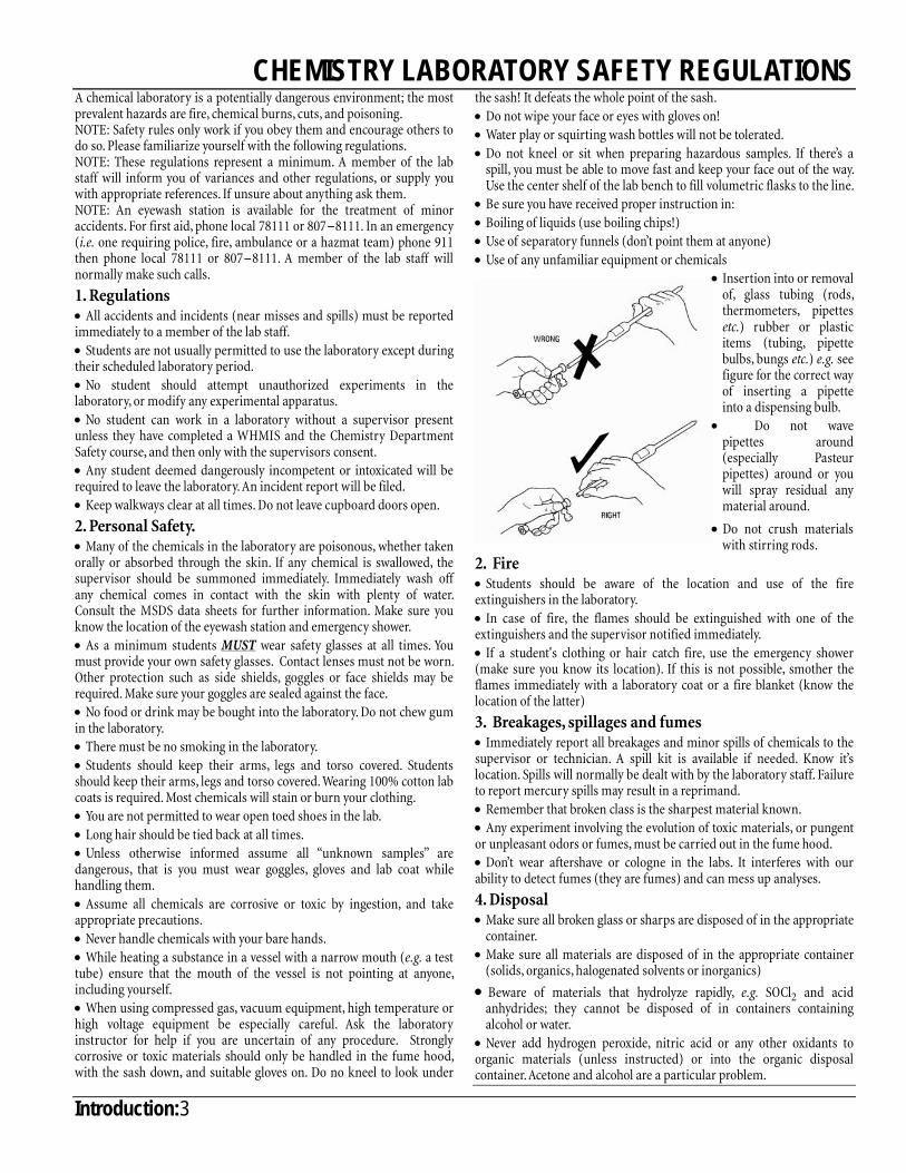
• Insertion into or removal of, glass tubing (rods, thermometers, pipettes etc.) rubber or plastic items (tubing, pipette bulbs, bungs etc.) e.g. see figure for the correct way of inserting a pipette into a dispensing bulb.
• Do not wave pipettes around (especially Pasteur pipettes) around or you will spray residual any material around.
• Do not crush materials with stirring rods.
2. Fire • Students should be aware of the location and use of the fire extinguishers in the laboratory. • In case of fire, the flames should be extinguished with one of the extinguishers and the supervisor notified immediately. • If a student's clothing or hair catch fire, use the emergency shower (make sure you know its location). If this is not possible, smother the flames immediately with a laboratory coat or a fire blanket (know the location of the latter)
3. Breakages, spillages and fumes • Immediately report all breakages and minor spills of chemicals to the supervisor or technician. A spill kit is available if needed. Know it’s location. Spills will normally be dealt with by the laboratory staff. Failure to report mercury spills may result in a reprimand. • Remember that broken class is the sharpest material known. • Any experiment involving the evolution of toxic materials, or pungent or unpleasant odors or fumes, must be carried out in the fume hood. • Don’t wear aftershave or cologne in the labs. It interferes with our ability to detect fumes (they are fumes) and can mess up analyses.
4. Disposal • Make sure all broken glass or sharps are disposed of in the appropriate
container. • Make sure all materials are disposed of in the appropriate container
(solids, organics, halogenated solvents or inorganics)
• Beware of materials that hydrolyze rapidly, e.g. SOCl2 and acid anhydrides; they cannot be disposed of in containers containing alcohol or water.
• Never add hydrogen peroxide, nitric acid or any other oxidants to organic materials (unless instructed) or into the organic disposal container. Acetone and alcohol are a particular problem.

Introduction:4
MARKING POLICIESAllocation of marks will be different from usual labs. and may vary with the experiment. As above, you start with one or two marks less than the maximum otherwise an unrealistic spread of marks will occur. The follow ‘items’ will be considered when marking labs.
TECHNIQUE. This mark will be assigned for things like speed (finishing time), sloppiness, preparation (did you read the lab. before arrival?), contribution to the laboratory discussions, breakage’s, record of original data in your lab. notebook, attentiveness and attitude, as well as pipetting, weighing, titrating and other standard lab. skills. These experiments are all straightforward and in many cases you have done them before so odd factors like attitude will weigh heavily – quietly sitting in a corner, noisily sitting in a corner, or slipping out for a pint – will be viewed dimly. Also, you will be marked on how you solved the problem and the computer techniques used; e.g. proper choice of data ranges, checking convergence criteria, use of special features rather than brute force (e.g. for Excel; in-cell iterations versus huge tables or use of named ranges).
RESULTS. Clearly, the better your technique, the better your results should be, but since some of these experiments are designed to produce bad results so you can use fancy techniques to fix them up a bit, this mark is a little odd. However, the experiments do often have built in checks, there are certain errors that can only be achieved by incompetence – this mark will address these.
PRESENTATION. This will be an opportunity to demonstrate your word-processing skills, HAND-WRITTEN REPORTS WILL NOT BE ACCEPTED for any lab. reports. You will be marked on presentation e.g. clear format, data properly identified, clear use of labels, proper choice of axes on graphs, clear comments (in Maple). Proper placement and sizing of titles, captions and graphs. You MUST record your original data and any in lab. notes in an approved lab. book. Do not submit this book with your reports, but I will wish to see it and assign marks according to it’s clarity and completeness. (The supplementary questions may involve a lot of pictures or derivation in that case it may be acceptable to hand-write that section – check with the instructor).
REPORT. See the appropriate section for a description of the format of your report. Most importantly, do example calculations for one sample and tabulate the final, and some intermediate data, for the rest of the samples. Be sure to
tabulate your original data points (that is working data point; for instance there is no need to reproduce the data from time-runs, only the data points that arises form the time-runs) at the start of the report. Also, at the end, tabulate your calculated results and the literature values. Error discussion is required for each lab. Error analysis may also be required. Make sure you indicate the algorithms used for doing calculations, particularly if you used a computer. Marks are given for extra background research and any insightful comments. (415 is a research based lab. so these are part of your main mark, not an opportunity for brownie points as with most labs.) Marks are deducted for; arithmetic errors, incorrect answers, failure to answer questions, failure to comment on results; incomplete error discussion, lack of literature values, bad organization and extreme untidiness, excessive neatness, and of course handing in the lab. report late. Be sure to answer all questions given. Not all reports are equally easy, marks allocated to a report may vary from 10 to 15 to 20, depending on the length and difficulty of the calculations and questions.
PROBLEMS. Some labs. have lots of questions to answer. In fact, some look like a lab. with a problem set attached to the end. The problems carry significant weight.
SAFETY. Normally, physical chemistry experiments are designed to work with safe chemicals and equipment. For advanced courses this is neither possible nor desirable. Place a small section in your lab. report giving toxicity information and precautions for each (and every one) of the chemicals used (starting material, products and by-products). Look it up, don’t guess. If you don’t take this seriously I won’t let you in the lab. However, remember to use credible sources as some sources tend to over exaggerate the hazards for legal reasons (i.e. beware of the manufacturers literature). The WHIMIS CD-ROM is a good place to start.
PLAGIARISM. See the separate section for details. Basically, if you copy from somebody else or allow somebody else to copy from you, you will get zero for that lab. report. Repeated infractions may get you suspended. Discussion of ideas is permitted, but the write ups must be independent.

Introduction:5
THE FORMAT OF A LABORATORY REPORTIDENTIFICATION. All labs. reports should have a front sheet that gives: Your name, the course number (Chem.309) and section no. Name of partner (if any). Full date of experiment (e.g. Tue. May 10th 2018). Experiment number. Lab. Profs. name.
TITLE. This should give both the substance or system studied and the method of physical measurement made, or of property determined.
OBJECT OR PURPOSE. One sentence; may not be necessary if it just duplicates the title.
PRINCIPLE OF METHOD. Briefly discuss the theory underlying the laboratory and briefly give the principle of the method, and use this as opportunity to write down any equations you will use in results and calculations.
PROCEDURE. You may refer to the lab. manual for this, but you should any modifications to the procedure and indicate possible improvements and sources of errors or other general problems. Draw diagrams of apparatus setup if required.
RESULTS AND CALCULATIONS. Tabulating usually saves a lot of time and space and keeps the prof. happy. Draw graphs using a computer, unless otherwise stated. Embed both the graphs and tables in the text. Be sure to make the graphs readable, say 6x5 in minimum size For repeated calculations, give one example and one only, in full. The example calculation should be embedded in the text, but may be hand written (try doing one by typing to see what a pain it is). This should come more naturally than in the past as you should be using Excel for calculations and will need to explain them. Make sure you always compare your results with the literature values when available. Make sure you indicate the algorithms or programs used for doing calculations.
DISCUSSION. This is a discussion of the results and their errors in the context of the data processing methods used. Benefits and shortcomings of the methods should be discussed.
ERROR DISCUSSION/ANALYSIS. For any quant-ity for which you have found a numerical value, give an estimate of error limits. Do not propagate the errors in your calculations unless an error analysis is required. Estimate random errors from observed scatter of data either visually, or by statistical computation. List possible sources of
systematic error, and estimate their limits (guesswork!). In general, don't make the discussion too detailed, unless you are told that an error analysis is required for that experiment. If you are told to do a full error analysis you need the formula in Table 3 of the Error Analysis section). For most purposes an error analysis using Table 2 of that section will suffice. Error analysis should be done along with your calculations. Discussion is done as a separate section.
CONCLUSIONS. Your major findings in a few lines. This section may not be necessary if you have them clearly set out at the beginning or end of the "discussion" section. Be sure that you have answered all questions in the text. Also, make any comments about the findings and there implications for errors in this and related experiments
QUESTIONS. The question may be in the body of the main body or given in a separate section at the end of the experiment. Clearly identify, separate and answer the questions at the end of your report. Do not embed the questions in the discussion or conclusions or in a long rambling paragraph at the end. Text answers should be typed. Numeric or algebraic questions can be hand-written.
REFERENCES. Place any references, in the standard A.C.S. format, in this section. WEB references, with the exception of the CHEMBOOK site are NOT acceptable. See the section on the Internet elsewhere.
Please feel free to discuss report format and other problems with the instructor, but do not expect detailed explanations or corrections written on your laboratory reports.
See the A.C.S. Authors Guide (in library) for further details on style and format of chemistry documents.

Introduction:6
SOME NOTES ON TYPE SETTING REPORTSAll lab. reports are to be typed using a computer. I recommend Word (and Word on the Mac at a push). Make sure the equation editor is installed (and you know how to use it). If you have last minute printing problems, see me, I may accept a disk copy. For the purposes of proofing your reports I recommend printing them out. I will supply you with a symbol font that contains nearly all the symbols you’ll need for chemistry, and a Greek font with some modifications suitable for scientific work (the standard symbol font has Greek characters, but they have to be italicized). I usually assign some keystrokes to a macro to turn them on or off. I will also give you some macros you might want to use. I want you to follow some basic typographic conventions for your report (or you’ll loose marks). They are as follows.
a) The main body of text should be in a proportionally-spaced (e.g. not Courier) western (e.g. not Cyrillic) serif font (e.g. Times New Roman, Garamond, School Book), not a sans serif font (e.g Arial) or any decorative font (e.g. Brush Script) or anything weird (e.g. Tekton). Use a normal face, not italicized, hollow or bold. Type size should be 12, 13 or 14pt. b) Titles should be bold, serif or sans serif, and larger than the main text; don’t bother with anything fancy. c) There should be a maximum of three fonts in a report (the main text, titles, symbols). If you want some variation on the title page you can use bold and italic (sparingly). d) Keep it simple, no curly borders or color (except maybe in graphs). Use bold or italic for emphasis, do not underline. e) Use tables for your data, don’t rely on tabs etc. Do not box the table, a couple of lines here and there usually does the job. f) Note that stuff like 13 CO3
2+ can only be typed in using the equation editor – learn to use it. g) The main body should be double or triple spaced (with a 1” margin all round) so I can insert comments. However, I will tolerate single spaced reports. h) Diagrams can be drawn by hand, but keep them neat. They should be captioned by a line of type. Equations must be typed in, I suggest you reference the manual (e.g. Exp. G eq.3) to reduce this burden. All graphs must be done by computer, but you can manually cut and paste them into your report if you wish (OLE works nicely, but only on fast machines with lots of memory). i) Do not cut and paste lumps of text from your partner’s reports. I want to see some originality; in both the content and the formatting (Also see the section on plagiarism).
j) Watch for l’s (ells) they look like 1’s (ones). In sans serif you get l’s (ells), 1’s (ones) and I’s (eyes). k) Number the pages just in case the staple falls out. If you need any help with word processing don’t hesitate to come and see me – it’s part of the course. Office 2007 is almost useless for lab. reports get a copy of Office 2003.

Introduction:7
TYPOGRAPHIC CONVENTIONS FOR PAPERSAll journals have conventions that you must adhere to in order to get a paper published in them. These conventions vary from journal to journal, although there are some common conventions to all journals. Below is a set of conventions that you must adhere to for your lab. report to be accepted. (These are over and above the format conventions laid out elsewhere in this manual). The conventions are based on those for A.C.S. journal and are detailed in the A.C.S. style guide (along with a grammatical guide and conventions for hyphenation, abbreviations, capitalization etc., well worth a peek at). Conventions for other journals are usually laid out in the front of the journal.
Fonts and case. • Use 12 pt Roman (or similar). • Do not used bold or italic except as indicated below. • Do not underline – ever. • Lower case Greek letters are always italicized. Upper
Greek letters case are not. • Mathematical variables and constants are italicized. • Numbers and operators are not italicized. • Vectors and tensors are bold. • Math variables are never case sensitive (like in the
moronic C). d and D are the same. • Element symbols are not italicized. • Use italics for emphasis. Use bold for titles. Increasing
font size is also useful for emphasis. • When defining a new word it is common to italicize it. • Italicize latinates (actually optional, but I tend to do it). • Try to make superscripts and subscripts 10pt (there’s a
macro on the disk for this). • Symbols and axis labels in graphs should be 12pt.
Abbreviations and units. • Units are never capitalized when spelt out. • Abbreviations for units should be spaced, e.g. 10 km hr-1
not 10km.hr-1. I tend to ignore this rule as it leads orphaned or widowed units.
• A list of approved abbreviations are in the A.C.S. Guide. • All abbreviations, except as listed below, must be defined
at their point of first use. a) The symbols for the elements. b) the latinates (i.e., e.g., etc.). c) at. wt., w/w, w/v, v/v, vol.
Layout. Consult the Format section for other details. • If the report is double-spaced I can insert comments
easily, but single space is OK. I use 14pt exactly. • Use one inch margins all round. That leaves some space
for comments. • Use a fly page. • Insert diagrams, graphs and tables into the text rather
than on separate pages. (Use cut and paste). • Number the pages. • Do not start sentences with numerals (use the word). • Breaks and indenting for paragraphs are your choice. • Number graphs, figures and tables clearly. • You should use the equation editor for equations.
Calculations can be inserted into the text in hand writing though (they are a real pain to type).
Equations, Tables & Figures. • Equation numbers should be at the left margin. The
equation should be centered. Refer to the equation as eq.n. • Label figures and tables underneath. The caption should
not exceed the with of the figure or table and should be centered. Refer to them as Figure.n or Table.n.
References. Any consistent referencing scheme will do, but the following is recommended. References should preferably be numbers and grouped at the end of the report. Do not use MS Word’s Endnote facility. Placing references in footnotes is ok though. References should be referred to by just a number in parenthesis or an author and a number.
Journals. 1) For sequentially numbered volumes : Name, M. Y.; Other, A.N. , Journal Abbrv. Year, volume, pages. . 2) For individually number volumes: Same, M. Y. , Journal Abbrv. Year, volume(issue), pages.
Books. 3) No editors: Name, M. Y.; Other, A.N. Title of the Book; Publisher: City, Year, Chap. or page refs. 4) Editor only: Title of the Book; Ed. Name; Publisher; City, Year, Chap. or page refs. 5) Author and editor: Author. A. N. In Title of the Book; Editor Name, Ed.; Publisher; City, Year, Chap. or page refs.
Web pages. You should not take reference material from the web as it is not peer reviewed and not a permanent medium. Do look around the page to see if it has a formal reference (most government pages will) or has a reference from which the material is taken. If not, note down the URL of the page and the date you obtained the information.
For reference to other types of materials see the A.C.S. style guide. (For which you have no reference, notice how irritating that is) – it’s in the library). Abbreviations for journal are also in the A.C.S. guide.

Introduction:8
TYPE SETTING TECHNICAL DOCUMENTS Introduction. For hints on typesetting in general, see Robin Williams book The Non-Designers Design Book. She also has a number of useful tips at www.eyewire.com/magazine/columns/robin. Some more information can also be found under www.microsoft.com/typography/ . The hints below refer specifically to type setting lab. reports. or lab. manuals. I’ve attempted to set up this page according to these hints, even if the rest of the manual is not setup that way (do as I say not as I do).
Emphasis and Titling. Do not use underline or ALL CAPS for emphasis or titling, they are a hangover from the typewriter days. However, I still find it useful to use a liberal sprinkling of DO NOT’s in lab. manuals.
For emphasis in text use italic, bold italic or bold. Occasionally, using a small font surrounded by white space works well as does using a larger font. For titling use a larger font, normal, bold or italic. If your main text is serif (as it should be) then a larger Sans Serif font is good. Placing a line across the page (as above) also works well in moderation. The lines may be various weights or doubled.
Typeface. If you are preparing a long document readability is very important. In print readability is best achieved by using a classic serif font such as Times Roman, Caslon, Garamond, Baskerville or similar (This manuals text is set in a slightly narrow Roman font – Adobe Minion). Don’t use anything fancy. If you are type setting a Web page or have a lousy printer then a san-serif font such as Arial may work better. I avoid Arial because of the confusion between I (eye) l (el) and 1 (one). Check for appearance on screen vs. the printer, the fonts named above (except Minion) look quite different on screen than they do in this text. Also, check the numbers for a given font in Times you get 1234567890 with Bulmer you get 1234567890, which is a little ugly (especially on screen).
In general, one should not use more than two or three typefaces per page, typically one for body text, one for titles, one for symbols. One may add one more font to represent computer or instrument input, Courier is usually used for that purpose.
Font Size. As can be seen in the section above that different fonts have different widths, heights, weights and spread, even though they have the same point size. Times is large and open and Caslon small and cramped so Times works well at 10pt, Caslon does not. On the other hand Caslon works fine at 14pt, and so does Times. I use 12pt for lab. manuals since they are usually read standing up (and I’m a little short sighted). For reports 10pt is ok if you have a laser printer, for inkjets 12pt is better.
Spacing. Spacing between lines is usually set to single (which is actually variable). For plain text this is ok, but is poor when you’re using super/subscripts or symbols. I find spacing at exactly 14pt (for 12pt text) works well if the “don’t center exact height lines” option in Word is off. If you’re writing a draft, double or triple spacing can be useful to allow for annotations.
Spacing between words is set by using left justification (no extra spacing) or by using full justification (spacing filled so line exactly fits the line). Full justification is fine as long as you don’t use narrow columns (a fine example of what can go wrong is in the opening paragraph).
Misc. Lines of text should not be more than (on average) eight-nine words long. For large format pages that means two or more columns. Large margins can also help. Setting up double columns can be a little awkward and slows down the computer. Some of the lab. manual is not set that way so I don’t expect it in lab. reports.

Introduction:9
PLOTTING GRAPHS. Most graphics packages give half decent graphs, however Excels defaults settings are setup for Business slides (i.e. for appearance not content.) However, the plots can be readily customized. Below are a set of refinements which can also be used to as general guidelines for plotting.
The top graph is Excels default scatter plot. The scales are wrong, the annotation too large and the plot cluttered. It is almost useless. You should setup a custom graph in a proper format and use that as the default..
For the first step we get rid of the grid lines (only leave grid lines if you need to read data of the graph) and the gray background which reduces contrast. The legend is also deleted. Again, legends are useful when working off the graphs, but for reports the legend should be below the graph along with other information. Note how the graph rescales when the legend is removed. Here we have removed the remaining background color and the joining lines. There is no measured data between the points so we can’t put a line there. We have also just changed the annotation to normal typeface. If you intend to reduce the figure you should scale the annotation accordingly. For reports annotation should match your text size (10-12pt). If you are making slides, overheads or reducing graphs, it will need to be bigger (18-24 pt often works). The title has been moved to the bottom and numbered. Most of these changes are accessible by left clicking on the graph, then right clicking to access the various properties.
The final step is to remove both figure and axis boxes, they serve no purpose. The title has been removed and replaced by text from Word because you can’t do anything fancy in Excel - in this case simply to put the legend in. Note that it is centered below the graph. The axes have been tidied up, the span has been corrected, decimal places reduced and tick marks added. The least square fit lines have been added. The data points have been changed to black and made easily distinguishable.
These graphs have been cut and paste in. If you do that, make sure they are a decent size, including the annotation. (see exp.P for some bad examples. Graphs can be presented on a separate page if necessary.
Figure 1. A plot of Cv vs. Vent time for the Clement – Desormes’. Dots at 20C, squares at 30C
Example Graph
0.0020.0040.00
-4.00 1.00 6.00
Time(s)
Spec
ific
Hea
t
Series1Series2
Example Graph
0.0020.0040.00
0.00 2.00 4.00 6.00
Time(s)
Spec
ific
Hea
t
Figure 1. Example Graph
0.00
10.00
20.00
30.00
40.00
0.00 1.00 2.00 3.00 4.00Time(s)
Spe
cific
Hea
t
20
25
30
35
0 1 2 3 4Time(s)
Spec
ific
Hea
t

Introduction:10
PRESENTING TABLES.
Time(s) P1 (cmHg) Cv 4.03 76.49 28.04099 3.25 76.67 26.34766 3.32 76.57 26.65888 3.06 76.73 26.85892 2.6 76.63 26 2.28 76.52 25.06601 1.75 76.6 25.01056 1.31 76.58 24.84336 0.96 76.6 24.65 0.66 76.51 24.25748
Time(s)
P1 (cmHg) Cv
4.03 76.49 28.04 3.25 76.67 26.35 3.32 76.57 26.66 3.06 76.73 26.86 2.60 76.63 26.00 2.28 76.52 25.07 1.75 76.60 25.01 1.31 76.58 24.84 0.96 76.60 24.65 0.66 76.51 24.26
Vent
Time(s) Pressure, P1
(cmHg) Cv
J/mol-1 4.03 76.49 28.0 3.25 76.67 26.4 3.32 76.57 26.7 3.06 76.73 26.9 2.60 76.63 26.0 2.28 76.52 25.1 1.75 76.60 25.0 1.31 76.58 24.8 0.96 76.60 24.7 0.66 76.51 24.3
Table 2. Vent times, initial pressure, P1, and calculated specific heat, Cv , for the Clement-Desormes experiment.
Excel’s default tables are nearly as poor as the graphs. Here we will illustrate how to tidy them up.
Generally you should cut and paste in from Excel in-line to the text, but if the table is very large it should be presented on a separate page, in landscape mode if neccessary. Either way the default cut & paste table is poorly laid out with lots of clutter and white space. Center the text and the table. The number of decimals are made uniform to clean up the appearance and allow a more meaningful column alignment and spacing. The heavy grid has also been removed. The grids can serve a purpose in large multicolumn data look-up table, but generally they just clutter the table.
The final step is to tidy up the table headings (centered vertically and horizontally) and add subscripts. Use the equation editor if necessary. A caption has also been added along with a light grid. Number formatting has been changed to reflect the correct number of significant figure. You may want to change the font type and size to match your text as well. A final note: Try to avoid E or exponential notation if necessary rescale your data to µM or whatever. e.g. use 0.234 not 2.34E-01 or 2.34x10⁻¹ (the latter is the lesser of two evils). Use 0.345µM, not 3.45x10⁻⁷M and certainly not 0.000000345M. Also remember to limit the number of decimal places, Excel defaults to something too large.

Introduction:11
USING FIGURESFigures are rarely prepared in situ they are usually prepared separately then cut and paste (manually or electronically) into the document. The only real exceptions are sketches in your lab. notebook. Regardless of the type of figure they all need a figure number and caption placed beneath it. The caption should be no wider than the figure. There are a number of ways of preparing figures for formal reports, each with advantages and disadvantages.
a) Hand drawn b) Drafted c) Computer drafted. d) Scanning.
Hand-drawn figures are not usually used in formal reports, but they are fast and convenient. Drafting involves special pens, templates, drawing boards etc. The usual approach is to draw an oversize figure and Xerox reduce it (that cleans it up a lot). You then manually cut and paste it into a prepared gap in the report and Xerox that page. This process is very labor intensive (the chem. dept at UBC has two graphic artists for this purpose), but it is the only way to do some types of pictures. Computer drafting moves all the drafting accessories onto the computer, however it can be difficult to do chemical drafting on the computer and the results are often unsatisfactory. It is most satisfactory if you have prepared templates of flasks etc. (CorelDraw has a good selection) or of rings and bonds (ChemDraw). Drawing pictures from scratch can be a real pain. Be sure to distinguish between CAD type programs (CorelDraw) used for drafting, and paint type programs (CorelPaint). The latter is good for pictures and tends to be poor for equipment figures. Computer figures can be printed out and manually cut and paste in or they can be electronically cut and paste in using OLE. OLE is the best way to go, you don’t loose resolution, but it sucks up computer resources. Also Corel has never mastered OLE so you can’t always use it. You can cut and paste in bitmap files from just about any program, but be careful as their resolution is limited (or they become so big they crash the computer). You need at least 600dpi resolution to reproduce line drawings properly.
Scanning is great – when it works. You use somebody else’s pictures and just cut and paste them electronically into you report. There are three problems though, one is copyright, they are, after all, somebody else’s pictures. Resolution is another, and color is the last. Copyright is usually not a problem for one-off lab. reports, but for anything you sell (such as lab. manuals) you have to get copyright permission, which may of may not be free. Resolution is a serious problem. Grayscale pictures may give acceptable results at 300dpi (check by printing a rough copy out), but even then they will be huge (on disk). Line drawings need at least 600dpi or you get jaggies. Scaling down often exacerbates the problem. Color also creates a problem. Most reports are in black and white with perhaps grayscale pictures. Color does not always converts to grayscale well, and almost never convert to good line drawings (black and white). Basically any picture with a colored background will be unusable. As an exercise go through this manual and see if you can determine which figures are hand drafted and scanned, computer drafted, scanned from other sources, bitmaps from other programs or OLE links.

Introduction:12
KEEPING A LABORATORY NOTEBOOKBasically, you need to record what, with what, when, where, how and how long, all in relation to your laboratory activities. An outline of the information you should record (by category) is given below (you don’t need to put such titles in the book). The laboratory book should have numbered duplicate pages. The duplicates should be removed and stored in a separate place from the laboratory book. If you have a laboratory, the laboratory book should be locked up in the laboratory. Keep the duplicates at home or in your office. Increasing amounts of data are kept on computers, be sure to backup the disks and record file names in your laboratory book. The lab. Manual contains some ‘NOTES’ sheets, they are an artifact of production. They are useful as scratch sheets, but anything of significance should be written in the lab. notebook, only. Incidentally, the examples given are real, not made up for your entertainment.
General a) Each page should be dated and titled. Start each new
date on a new page, unless the entries are less than ¼ of a page. The title should be short, but descriptive and placed in an index at the front of the book.
b) Entries should be neat and in water insoluble pen. c) Entries should be organized – start new topics on a new
line. d) Mistakes should be deleted with one line (leaving the
mistake clear – it might not be a mistake). Do not delete or change entries after the fact.
e) Place any literature references against appropriate entries.
f) Note any modifications to any standard procedures. g) Keep your notes legible. Dalton may have been a great
chemist, but his lab. notes weren’t that great as seen below.
Pre-Laboratory Preparation. a) Write in any directions, calculations, diagrams, flow
charts, molecular weights, cautions, weights and volumes.
Instruments a) Record instrument settings (scan time, resolution, scan
width, temp. etc. etc. – anything that can be varied). Anything that doesn’t have a value, indicate any changes. E.g. lamp height was optimized for the standard sample.
b) State sample cells used (try and get your own). If they break record that (different cells give different results).
c) If there are any power glitches or the signal seems very noisy, indicate those along with the time. E.g. at UBC it used to be impossible to work at 4.30, when everybody was turning their instruments off. There was also trouble with big lasers firing; recording times will help you track these things down.
d) Record the computer file names that any data is held in. Make them useful, have a convention. If the OS supports long file names use them. I find it useful to use a convention like XXYYnnnn.mmm – where XX is a two letter month code, YY is the day (number), nnnn is a code for the experiment/sample type, mmm is the extension, usually you won’t have a choice about that. E.g. JL09dx12.spc might mean a spectrum (spc) taken July 09, of a doxyl-12 spin probe. Most computers are pretty good about keeping the file date correct so you may want to just use an 8-letter code instead. However, it’s often easier to search for a file name than for a file date. I like to use an extension nnn where nnn was 000, 001, 002 etc. for a sequence of files. It can be very difficult to locate three month old data, especially if you generate 100 files a day.
Preparation a) Record the chemicals, grades, weights and volumes
used. b) Record the order in which the chemicals were added. I
once did a preparation with three chemicals, which gives three possible orders (assuming the order of a given pair is irrelevant). Not only did two of the combinations give the wrong product, the reactions were explosive. The order was not given in the original instructions.
c) Draw, or otherwise indicate the equipment used. (Some reactions depend on the size and shape of the flasks). Something a little more auspicious that the efforts of the Greek alchemist shown below, but drafting is not required.

Introduction:13
d) If any of the bottles have old labels, broken caps, or discolored contents, record that. Some chemicals just don’t work when old. Hydrogen peroxide is really bad for that, check the bottle date.
e) Record any changes to the preparation procedures. E.g. 200mL flask used instead of recommended 50mL flask.
f) Note the course of reaction and other details. E.g. 1) reaction proceeded smoothly and was complete in 10mins. 2) Reaction proceed rapidly and blew a bung out (replaced rapidly). 3) Some silicone grease dripped into the reaction vessel. 4) Reaction turned green after 30 min (instead of yellow at 45min.). Mixture detonated after 32min. (The student who noted the latter dropped chemistry and became a lawyer). 5) Initial preparation showed traces of NO2. Reaction vessel was flushed with nitrogen again to remove oxygen. 6) Foul smell, sample stored in fume hood.
Times Time is more important than you think. One preparation in my laboratory, at UBC, didn’t work on sunny winter days, but worked fine on sunny summer days. This was because the sun would shine into the laboratory at 4pm, in winter, just when the silver salts were added to the reaction (it was an 8hr prep.). In the summer, the sun was to high to shine in. Record reaction times, flushing times, reflux times, start times, end times, just about any time you can think of.
Results a) Record basic physical data; total mass, state, % yield,
m.p.t. etc. b) Record any other data including program and version
number, if the result is produced by a computer. Be sure to record any file names.
Miscellany Record anything else you notice. e.g. 1) samples were yellow when removed from freezer, but turned a transient red
(almost a flash) then went pale yellow, the color before freezing. (In this case the pale yellow turned out to be iron contamination from the cheap stainless steel syringe needles used to deliver into reactants to the sample). 2) Fine white needles formed in the acetone wash bath after two days of use. (They turned out to be acetone peroxide, a contact explosive, even when wet).
Computers. REMEMBER TO BACK UP ALL YOUR COMPUTER DATA IMMEDIATELY. Computers generate huge amounts of information and it’s silly to reproduce it in a notebook. There are some exceptions, X-ray data and spectra typically find their way into special libraries. For your work, you can restrict yourself to the following items. a) Record filenames used in a given experiment. Record
any data that the instrument doesn’t put into it’s files. b) If doing simulations setup a table of filenames, input
parameters and comments on success or whatever. c) Computers are finicky, record any difficult to remember
procedures (say for importing data) into your book. d) Paste in things like ASCII tables or program procedures
into the lab. book. e) Record the computer type and program version nos.
Bugs are often undetected for a long time, this data will help you decide their relevance.
f) Make sure you indicate the algorithms used for doing calculations, particularly if you used a computer.
INTRODUCTION:14 © P.S.Phillips 2011 October 31, 2011
PLAGIARISM
You cheat, You’re dead meat.
For a detailed discussion of plagiarism see the OUC Guide to Plagiarism available from the bookstore. The policy is basically one of zero tolerance. The penalty for plagiarism is usually a zero for the work involved and a letter of reprimand. Penalties for theft of papers or repeated plagiarism may be expulsion. Avoiding plagiarism in chemistry labs. is quite simple; don’t copy other peoples work ! That is, do not copy or read the whole or sections of another person laboratory report, draft or final.
There are cases where it is acceptable to copy other peoples work, in which case you should note the following:
a) If you wish to copy blocks of text from some source, put it in quotes and reference the source. You should not do this a lot or you will be penalized for poor style. The source of material must not be another students lab. report or from a ‘tutoring service’.
b) If you use any source to assist in writing your labs. make sure you reference those sources in your write up. If you paraphrase the text from these sources, try to do it as loosely as possible (i.e. keep it close to your personal style). If the paraphrasing is too similar to the original you may be open yourself to a plagiarism charge. I find it best to read two or more sources, close those sources and then write out what I understand of what I’ve just read. Again, the sources must not be other students lab. reports, profs. notes etc.
c) You may discuss labs. with other students and you may compare original data and graphs. At a pinch, you can compare calculations to track down errors. Under no circumstances should you read or copy other students lab. reports (final or draft), that is considered plagiarism. If you read another students report (but not necessarily copy) it will taint the style of your write up. It is quite shocking how easy that is to detect, particularly is small classes – so don’t do it!
d) Do not copy other students graphs or tables either electronically or by Xeroxing. Producing your own graphs and tables is an important part of this course. (This may be acceptable in other courses, but not this one).
See the supplementary information on others marks penalties.
HOUSE KEEPING Before starting an experiment, wash, and if necessary dry, any glassware, before use. Remember, the last person to use the glassware was a student.
At the end of the experiment be sure to clean and wash any glassware. If you found it on the bench, in the cupboard, the draws, the outside and return it there. If it came from a stock cupboard , put it on the drying rack. Make sure you leave the balances clean. If any equipment was disassembled when you got it, disassemble it again and return to where you found it. Leave any equipment or chemicals that the instructor/technician gave you on the bench. Clean up any spills, paper towels, or any other mess you make. Report any breakages or depleted reagents so we can make replacements. Failure to do this housekeeping may result in marks being deducted.

© P.S.Phillips October 31, 2011 ERROR ANALYSIS:1
INTRODUCTION TO ERROR ANALYSIS INTRODUCTION. There is a hierarchy of error analysis. Each step being successively more rigorous.
i) sigs figs ii) simple addition of errors ii) addition of squares of errors iv) series expansions to estimate errors v) calculus
Although each step is more rigorous, they are less conservative. i.e. sig. figs always overestimates the errors. Note that each case requires a prior estimate of the error. If you have to estimate the error from your data set (typical in the earth, life and social sciences) then you must resort to statistics. All quantitative chemistry experiments should incorporate a check using significant figures. For error analysis usually simple addition of errors will suffice, although one may have to resort to series expansion of functions to do that.
I. SHORT CUTS IN ERROR ANALYSIS: A NOTE ON SIGNIFICANT FIGURES. Error analysis is a pain so if we assume all the errors are +1 in the last reported figure of the data, then the error analysis is greatly simplified: One just counts significant figures or decimal places and propagates those according to the rules familiar to you from first year chemistry and physics. At this stage of life, you should do significant figures instinctively. However, the glowing display on your calculators seems to interfere with this process so here are a couple of rules to stop you going too far wrong.
1) Never, ever write down all 10-12 figures off the calculator, but feel free to carry that number in your calculations.
2) Computers/calculators often do not do calculations to more than 5-6 sig. figs. for functions Even though they may print out more.
Never quote errors to more than two sig. figs. One sig. fig. will often suffice. e.g. 56.74+1.32 becomes 57+1, 1032.4+1.3% becomes 1.03x10³+1%. Also you must get the sig. figs. right. An error is a + quantity so follows the rules for addition/subtraction; that is the number of decimal places in your error must match those of the error.
3) If your using volumes in calculations you will never have more than four sig. figs. Usually three after subtractions.
4) If your using weights (in our labs.) you will never have more than six sig. figs. Usually only five after subtractions.
5) Atomic masses are often only good to three sig. figs. due to variations in isotopic composition.
6) If you worry about how many sig. figs. to carry in calculations, carry six, although four is often adequate. (In general, carry one more sig. fig. than you know the answer will generate).
7) Significant figures underestimate the true error so beware that reasonable significant figures may hide a gross error. If you’re down to 2 sig. figs. you should consider doing an error analysis to see if the data actually means anything.
8) Remember sig. figs. only apply to simple math operations. If functions are involved you will have to resort to proper error analysis, at least for that step in the calculation. Watch polynomials in x, in particular, if x<1 then the high order coefficients. need less sig. figs than the lower order ones. If x>1 then the high order coefficients need more sig. figs. Both Excel and Origin have a bad habit of reporting polynomial coefficients with insufficient significant figures. Work out how to reset that.
9) One notable exception to sig. figs, of functions are logs. The leading number carries the exponent so has now error. Thus, the log, 3.13 has two sig. figs., the 3 just tells you to multiply by 1000.
10) Soooooo, unless you have a very good reason (e.g. you are measuring frequencies) never write numbers down to more than 6 sig. figs. In addition, you never write a final answer down to more than four sig. figs, in fact three will do in many cases. IN ADDITION, do the proper sig. figs, don’t just blindly write down three or four sig. figs at each step and don’t give errors more than two (preferably one) sig. fig.
A short cut, but one that requires a fair amount of competence and experience in error analysis, is to break the calculations down into small steps and try to identify where the largest error occurs (Actually it’s always a good idea to do this before the experiment then you know where to focus your attention). Often this error will be so much larger than all the other errors that you can ignore them, i.e. you only need propagate the one error. The most common example of this is where you mix volumes and weights in a calculation. Weights are 2-3 orders of magnitude more precise than volume so you often only need propagate the volume errors.
II. ERRORS. All measurements are associated with some kind of error or uncertainty. We never know exactly how big
ERROR ANALYSIS: 2 © P.S.Phillips October 31, 2011
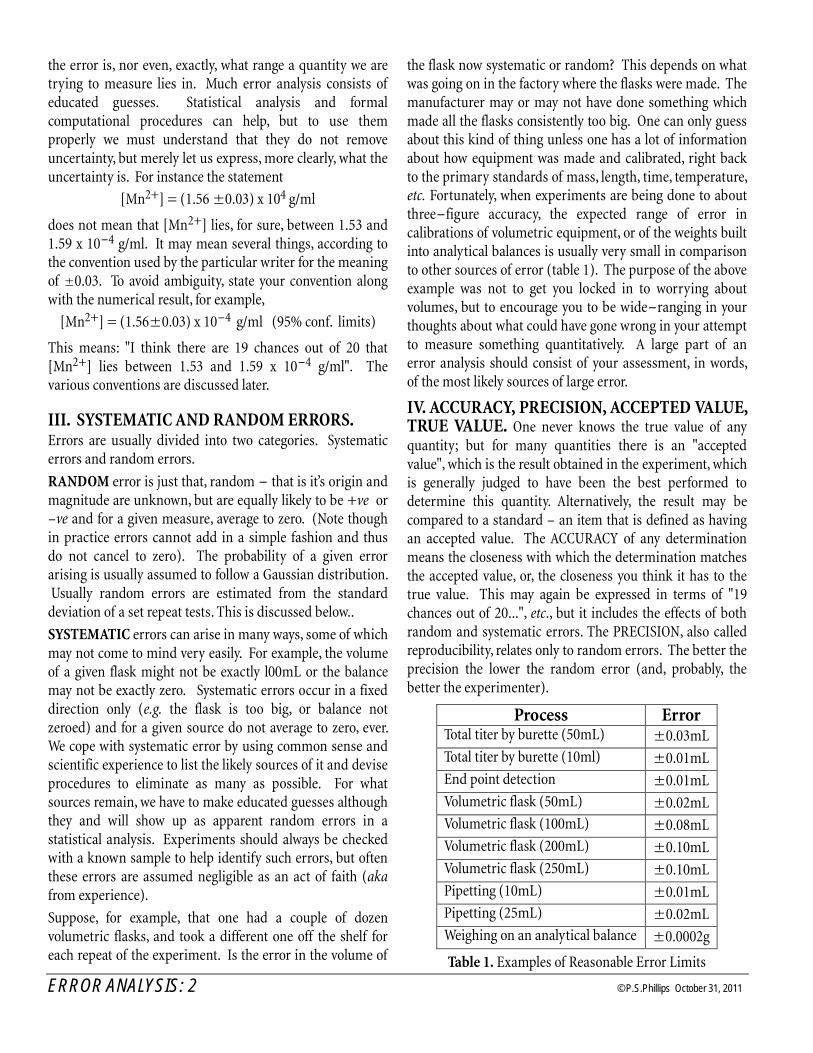
the error is, nor even, exactly, what range a quantity we are trying to measure lies in. Much error analysis consists of educated guesses. Statistical analysis and formal computational procedures can help, but to use them properly we must understand that they do not remove uncertainty, but merely let us express, more clearly, what the uncertainty is. For instance the statement
[Mn2+] = (1.56 +0.03) x 104 g/ml
does not mean that [Mn2+] lies, for sure, between 1.53 and 1.59 x 10⁻⁴ g/ml. It may mean several things, according to the convention used by the particular writer for the meaning of +0.03. To avoid ambiguity, state your convention along with the numerical result, for example,
[Mn2+] = (1.56+0.03) x 10-4 g/ml (95% conf. limits)
This means: "I think there are 19 chances out of 20 that [Mn2+] lies between 1.53 and 1.59 x 10⁻⁴ g/ml". The various conventions are discussed later.
III. SYSTEMATIC AND RANDOM ERRORS. Errors are usually divided into two categories. Systematic errors and random errors.
RANDOM error is just that, random - that is it’s origin and magnitude are unknown, but are equally likely to be +ve or –ve and for a given measure, average to zero. (Note though in practice errors cannot add in a simple fashion and thus do not cancel to zero). The probability of a given error arising is usually assumed to follow a Gaussian distribution. Usually random errors are estimated from the standard deviation of a set repeat tests. This is discussed below..
SYSTEMATIC errors can arise in many ways, some of which may not come to mind very easily. For example, the volume of a given flask might not be exactly l00mL or the balance may not be exactly zero. Systematic errors occur in a fixed direction only (e.g. the flask is too big, or balance not zeroed) and for a given source do not average to zero, ever. We cope with systematic error by using common sense and scientific experience to list the likely sources of it and devise procedures to eliminate as many as possible. For what sources remain, we have to make educated guesses although they and will show up as apparent random errors in a statistical analysis. Experiments should always be checked with a known sample to help identify such errors, but often these errors are assumed negligible as an act of faith (aka from experience).
Suppose, for example, that one had a couple of dozen volumetric flasks, and took a different one off the shelf for each repeat of the experiment. Is the error in the volume of
the flask now systematic or random? This depends on what was going on in the factory where the flasks were made. The manufacturer may or may not have done something which made all the flasks consistently too big. One can only guess about this kind of thing unless one has a lot of information about how equipment was made and calibrated, right back to the primary standards of mass, length, time, temperature, etc. Fortunately, when experiments are being done to about three-figure accuracy, the expected range of error in calibrations of volumetric equipment, or of the weights built into analytical balances is usually very small in comparison to other sources of error (table 1). The purpose of the above example was not to get you locked in to worrying about volumes, but to encourage you to be wide-ranging in your thoughts about what could have gone wrong in your attempt to measure something quantitatively. A large part of an error analysis should consist of your assessment, in words, of the most likely sources of large error.
IV. ACCURACY, PRECISION, ACCEPTED VALUE, TRUE VALUE. One never knows the true value of any quantity; but for many quantities there is an "accepted value", which is the result obtained in the experiment, which is generally judged to have been the best performed to determine this quantity. Alternatively, the result may be compared to a standard – an item that is defined as having an accepted value. The ACCURACY of any determination means the closeness with which the determination matches the accepted value, or, the closeness you think it has to the true value. This may again be expressed in terms of "19 chances out of 20...", etc., but it includes the effects of both random and systematic errors. The PRECISION, also called reproducibility, relates only to random errors. The better the precision the lower the random error (and, probably, the better the experimenter).
Process Error Total titer by burette (50mL) +0.03mL Total titer by burette (10ml) +0.01mL End point detection +0.01mL Volumetric flask (50mL) +0.02mL Volumetric flask (100mL) +0.08mL Volumetric flask (200mL) +0.10mL Volumetric flask (250mL) +0.10mL Pipetting (10mL) +0.01mL Pipetting (25mL) +0.02mL Weighing on an analytical balance +0.0002g
Table 1. Examples of Reasonable Error Limits

© P.S.Phillips October 31, 2011 ERROR ANALYSIS:3
V. USING OF STANDARD DEVIATION AS THE ERROR. The most common way of characterizing random error in a data set is the standard deviation. The true standard deviation for a population is of n observations of a variable x is
22 1lim ( )x i x
nx
ns m
®¥= -å
where µx is the true or population mean. This is sometimes written
22 1( )x ix x
Ns = -å
where it’s understood that N (as opposed to n) is the true population size and not the sample set size, and x is the mean (equals the population mean as N is the population size). In practice, µx is unknown and is calculated for the data; the limit on n ensures that x approaches µx, the true (population) mean. If n is small, then the standard deviation and average are no longer independent as, given n-1 data points and x , the nth data point can be calculated, we have lost a degree of freedom. To account for this we must reduce the sample size by one so
22
1
( )
1
ni
xi
x xsd
n=
-=
-å
Here n is the sample size, x is the mean of the sample set (an estimate of µx) and sd the standard deviation (an estimate of σx).
If n is large and we know µx then any difference between µx and x can be attributed to a systematic error. If n is small then x is inherently unreliable. We can estimate the reliability of the mean by using the standard error on the mean, σm, which is given by
σm = σ / n ½
σm tends to zero for large n. i.e. we can thus improve our estimate of the average by collecting more data points. Do not confuse the standard error on the mean with the standard deviation. The former is a measure of the error of estimating of the mean (i.e. accounts for the fact that the sample size and population size differ); the latter is a measure of the spread (or error) of the data
CALCULATING STANDARD DEVIATION. For the purpose of calculation, it’s convenient to make the following assignments
2( )xx iS x x= -å 1
xxx
SV
n=
-
and x xsd V=
However, it’s inconvenient to calculate Sxx using the above formula so it’s often calculated using the mathematically equivalent formula
( )22 1xx i iS x x
n= -å å
While this is algebraically equivalent, it’s not computationally equivalent. The former method requires lots of storage memory so the latter method tends to be used on calculators. However, the latter method is subject to round-off errors so you can get quite wildly different vales for the standard deviation with different calculators so be warned. An interesting variation in calculating the standard deviation is as follows
( )1
221
1
1
2( 1)
n
i ixi
x xsdn
-
)=
-=- å
In the absence of systematic errors (such as drift or rolling baseline), this reduces to the normal value for the sd. However, in the presence of drift (low frequency noise) it gives the sd. associated with high frequency noise. (i.e. it is robust wrt. to drift). This is useful for identifying ‘noise’ in the presence of drift. Furthermore, this is a running measure, that is, it can be easily calculated as the data is acquired. The usual sd. requires you to constantly recalculate the mean.
CONFIDENCE LIMITS. If the data is normally distributed, then the standard deviation is just the half-width of the normal curve at half-height. While this is a convenient measure of the normal curve, much of the data lays in the tails of the curve. Roughly, one in three points lay outside the +1sd limit of the curve or to put it another way, there’s only a 2 in 3 chance that the true mean lies within the quoted limits. For some reason, this bothers some people and they prefer to use wider error limits, for instance +2sd. That is, limits such there are 19 chances out of 20 that the true value of the mean lies within the limits. Occasionally you will see +3sd, or 99 chances out of hundred. Because of this, it is necessary to state the so-called confidence limits for your error so
3.5+1.0 (68% confidence limits)
means 3.5 with a standard deviation of 1.0
3.5+1.0 (95% confidence limits)
means 3.5 with a standard deviation of 0.5
3.5+1.0 (99% confidence limits)
means 3.5 with a standard deviation of 0.33

ERROR ANALYSIS: 4 © P.S.Phillips October 31, 2011
For our purposes, we will just use first method, i.e. one standard deviation and the limits not explicitly stated. A more rigorous approach is recognize that for small data sets the errors are not normally distributed, they are distributed according to the Student-t distribution. The confidence limits should then be written c
d xx t sd± where cdt is the t
value for a confidence limit of c (0.1 for 90%, 0.05 for 95% etc.) and d degrees of freedom (number of data points –2, which you should quote in your results).
OUTLIERS. Sometimes you obtain data that’s way outside the expected range of values. Such data points are called outliers. There are three reasons for spurious data i) It’ s real: While the probability of a data point beyond the five s.d. limit is small, it is still finite so occasionally you can expect an odd point. ii) It is real: The data distribution is not normal. For example, the data may be distributed with a Poisson or Lorentzian distribution, both of which have long tails. Under such circumstances, outliers can be quite common. iii) It is due an error, e.g. contamination, power bumps. The last case is the most common cause of outliers and for that reason outliers are often just thrown out. The problem is that it is not always clear that the data is a glitch or that it is even an outlier. For highly scattered data, one should always do an outlier test before rejecting a point. Also, remember that it may be real data. Although it may be necessary to throw the point out to keep your statistical analysis valid, that data point may contain information. For instance in soil sampling that point may represent an ore deposit (in fact ore deposit are detected by looking for outliers). In medicine, the data point may be due to a diseased specimen, in which case your analysis may provide a diagnostic for that disease.
My personal preference is to leave outliers in and use robust estimation methods, which are, by definition, insensitive to outliers. If your analysis methods are automated in any way you should use robust methods, because it is very difficult to automate outlier rejection in noisy data.
VI. ERROR ANALYSIS. Although the following is a more rigorous approach to error analysis than you will see in first year chemistry texts and will suffice for our needs, you should be aware that there are still a number of approximations made. Briefly, they are as follows: It is assumed that the errors are random and distributed in a normal fashion (this will usually be true if outliers are rejected). It is assumed that the errors are small ~1% (and certainly <10%. If not then the error will be generally larger than calculated). It is assumed that the errors are derived
from a sample population that is sufficiently large to be reliable and is representative.
Error analysis usually refers to analysis the effect of random errors, not systematic errors. While it is useful to ask questions such as “If the flask was to big, how will that affect the measured density”, it’s not useful to ask such questions in a quantitative fashion. After all, if you know how big a systematic error is, it has ceased to be an error.
ERROR PROPAGATION FOR A PRODUCT OF TWO FUNCTIONS. Consider two functions f(x) and f(y) each with small errors associated with the variables, i.e. f(x+δx) and f(y+δy). What is the error for the product of the two functions? If the errors are small, and the functions well behaved, then we can expand them about the average value of x and y using the Taylor series. So for f(x)
2 ''( )( ) ( ) . '( )
2
f xf x x f x x f x xd d d± = ± ± )
If the function is smooth then f ’’(x) will be small and if the error is small so will be δx so we can ignore higher order terms so
( ) ( ) . '( )f x x f x x f xd d± » ±
Thus for the product of f(x) and f(y), w= f(x) f(y), we get (including the errors)
= ( ) ( )
( ( ) . '( ))( ( ) . '( ))
w + w f x x f y y
f x x f x f y y f y
d d dd d
± ±» ± ±
( ) ( ) ( ) '( )
( ) '( ) '( ) '( )
f x f y f x f y y
f y f x x f y f x x y
dd d d
= ± ±±
Again, for small errors and a smooth function we can drop the last term.
'( ) '( )( ) ( ) 1
( ) ( )
f y y f x xf x f y
f y f x
d dæ ö÷ç ÷» ± ±ç ÷ç ÷çè ø
thus '( ) '( )
( ) ( )
f y y f x xw
f y f x
d dd » ±
For the simple functions f(x)=x and f(y)=y this reduces to the simple rule that the error is the sum of the fractional errors. i.e.
( ) ( ) 1y x
f x f yy x
d dæ ö÷ç ÷» ± ±ç ÷ç ÷çè ø
thus y x
wy x
d dd »± ±

© P.S.Phillips October 31, 2011 ERROR ANALYSIS:5
The + implies that the errors could mysteriously cancel out which is not the case so it’s usual to ignore the signs of the errors and write
y xw
y x
d dd » )
This overestimates the error, but will be dealt with more rigorously below. For more complex functions we need to incorporate the derivative, this will also be dealt with below. For basic error propagation the formula below suffice.
Operations and Errors Addition or Subtraction Z = A + B + C+.…
∆Z =| ∆A| + |∆B| + |∆C|+….
Multiplication or Division Z = A.B.C….
|∆Z/Z| = |∆A/A| + |∆B/B| + |∆C/C|+….
General Z = f(A,B,C….)
|∆Z| = |∆A.df/dA| + |∆B.df/dB| + |∆C.df/dC|+….
ERROR PROPAGATION FOR MULTIDIMENSIONAL FUNCTIONS. We could proceed as above, but it slightly clearer to use the chain rule. To calculate the effect of a small error we need to examine the effect of the error on (i.e. small changes in) the function, which is the same questions as what is the size of the derivative of the function with respect to each of it’s variables. For a function w=f(x,y,z) we have that
, ,,
( , , ) ( , , ) ( , , )
y z y xx z
f x y z f x y z f x y zdw dx dy dz
x y z
öö ö¶ ¶ ¶÷÷ ÷÷= ) )÷ ÷÷÷ ÷÷ø ø¶ ¶ ¶ø
If the errors are small, we can approximate dx to δx etc. This is equivalent to dropping the high order terms in the Taylor expansion. It’s thus straightforward to get the error for such function. Also, if we recognize that the product, xy, is a multidimensional function, f(x,y), it’s easy to see how to get the error for a product.
VII. USING THE STANDARD DEVIATION AS THE ERROR. The error is not a simple number, it can have any number of values, it is in fact a characteristic parameter for a probability distribution of possible errors, it is not the error itself. Assuming the errors are normally distributed and that sufficient data has been collected, the standard deviation of the data will be width of the normal distribution. Since the errors for each term maybe +ve or -
ve they will tend to cancel, but not completely, as that would require all the errors to have their signs anti-correlated, not a very likely event. To take this into account we proceed as follows: Consider that we want to determine quantity w, that is a function of at least two variables, so that w=f(x,y…..). We can determine a value of wi for each measured set of values so that wi=f(xi,yi,…). Now we wish to get the standard deviation of w
22 1( )w iw w
Ns = -å
xi-x is the error for a given measurement so assuming it’s small we can expand the error in w via the chain rule so that
( ) ( )i i iw w
w w x x y yx y
æ öæ ö¶ ¶ ÷ç÷ç ÷- - ) - )ç÷ç ÷÷ç ç ÷çè ø¶ ¶è ø
hence 2
2 1( ) ( )w i i
w wx x y y
N x ys
é ùæ öæ ö¶ ¶ ÷ç÷ê úç ÷- ) - )ç÷ç ÷÷ê úç ç ÷çè ø¶ ¶è øë ûå
222 21
( ) ( )
2( )( )
i i
i i
w wx x y y
N x y
w wx x y y
x y
æ öæ ö¶ ¶ ÷ç÷ç ÷= - ) - )ç÷ç ÷÷ç ç ÷çè ø¶ ¶è øæ öæ ö¶ ¶ ÷ç÷ç ÷- - )ç÷ç ÷÷ç ç ÷çè ø¶ ¶è ø
å
If we now define a covariance between x and y, σxy, as
2 1( )( )xy i ix x y y
Ns - -å
so we get for the error propagation function
222 2 2
2 2
w x y
xy
w w
x y
w w
x y
s s s
s
æ öæ ö¶ ¶ ÷ç÷ç ÷) )ç÷ç ÷÷ç ç ÷çè ø¶ ¶è øæ öæ ö¶ ¶ ÷ç÷ç ÷) )ç÷ç ÷÷ç ç ÷çè ø¶ ¶è ø
If x and y are uncorrelated then we expect that, on average, the covariance will be zero (there will be an equal number of +ve and –ve values in the sum) and we may neglect the last term giving us
222 2 2w x y
w w
x ys s s
æ öæ ö¶ ¶ ÷ç÷ç ÷) )ç÷ç ÷÷ç ç ÷çè ø¶ ¶è ø
Which for the simple case of the product of x and y (w = xy) this reduces to
2 2 2w x ys s s) )
i.e. we sum the squares of the errors, to get the total error.
ERROR ANALYSIS: 6 © P.S.Phillips October 31, 2011
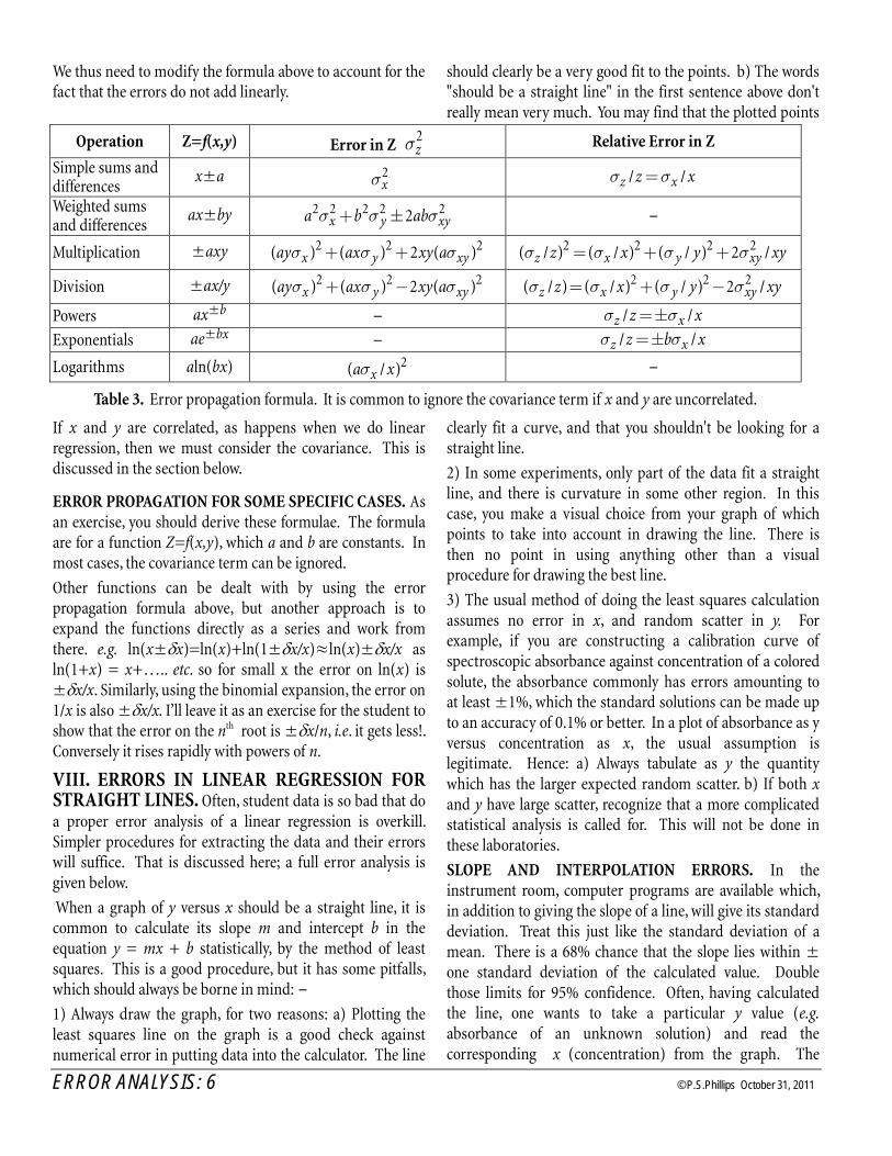
We thus need to modify the formula above to account for the fact that the errors do not add linearly.
If x and y are correlated, as happens when we do linear regression, then we must consider the covariance. This is discussed in the section below.
ERROR PROPAGATION FOR SOME SPECIFIC CASES. As an exercise, you should derive these formulae. The formula are for a function Z=f(x,y), which a and b are constants. In most cases, the covariance term can be ignored.
Other functions can be dealt with by using the error propagation formula above, but another approach is to expand the functions directly as a series and work from there. e.g. ln(x+δx)=ln(x)+ln(1+δx/x)~ln(x)+δx/x as ln(1+x) = x+….. etc. so for small x the error on ln(x) is +δx/x. Similarly, using the binomial expansion, the error on 1/x is also +δx/x. I’ll leave it as an exercise for the student to show that the error on the nth root is +δx/n, i.e. it gets less!. Conversely it rises rapidly with powers of n.
VIII. ERRORS IN LINEAR REGRESSION FOR STRAIGHT LINES. Often, student data is so bad that do a proper error analysis of a linear regression is overkill. Simpler procedures for extracting the data and their errors will suffice. That is discussed here; a full error analysis is given below.
When a graph of y versus x should be a straight line, it is common to calculate its slope m and intercept b in the equation y = mx + b statistically, by the method of least squares. This is a good procedure, but it has some pitfalls, which should always be borne in mind: -
1) Always draw the graph, for two reasons: a) Plotting the least squares line on the graph is a good check against numerical error in putting data into the calculator. The line
should clearly be a very good fit to the points. b) The words "should be a straight line" in the first sentence above don't really mean very much. You may find that the plotted points
clearly fit a curve, and that you shouldn't be looking for a straight line.
2) In some experiments, only part of the data fit a straight line, and there is curvature in some other region. In this case, you make a visual choice from your graph of which points to take into account in drawing the line. There is then no point in using anything other than a visual procedure for drawing the best line.
3) The usual method of doing the least squares calculation assumes no error in x, and random scatter in y. For example, if you are constructing a calibration curve of spectroscopic absorbance against concentration of a colored solute, the absorbance commonly has errors amounting to at least +1%, which the standard solutions can be made up to an accuracy of 0.1% or better. In a plot of absorbance as y versus concentration as x, the usual assumption is legitimate. Hence: a) Always tabulate as y the quantity which has the larger expected random scatter. b) If both x and y have large scatter, recognize that a more complicated statistical analysis is called for. This will not be done in these laboratories.
SLOPE AND INTERPOLATION ERRORS. In the instrument room, computer programs are available which, in addition to giving the slope of a line, will give its standard deviation. Treat this just like the standard deviation of a mean. There is a 68% chance that the slope lies within + one standard deviation of the calculated value. Double those limits for 95% confidence. Often, having calculated the line, one wants to take a particular y value (e.g. absorbance of an unknown solution) and read the corresponding x (concentration) from the graph. The
Operation Z=f(x,y) Error in Z 2zs Relative Error in Z
Simple sums and differences
x+a 2xs / /z xz xs s=
Weighted sums and differences
ax+by 2 2 2 2 22x y xya b abs s s) ± -
Multiplication +axy 2 2 2( ) ( ) 2 ( )x y xyay ax xy as s s) ) 2 2 2 2( / ) ( / ) ( / ) 2 /z x y xyz x y xys s s s= ) )
Division +ax/y 2 2 2( ) ( ) 2 ( )x y xyay ax xy as s s) - 2 2 2( / ) ( / ) ( / ) 2 /z x y xyz x y xys s s s= ) -
Powers ax+b - / /z xz xs s=±
Exponentials ae+bx - / /z xz b xs s=±
Logarithms aln(bx) 2( / )xa xs -
Table 3. Error propagation formula. It is common to ignore the covariance term if x and y are uncorrelated.

© P.S.Phillips October 31, 2011 ERROR ANALYSIS:7
programs again give an error limit, which should be treated as standard deviation and doubled for 95% confidence.
If there are large errors or outliers in the data, it is better to use a robust linear regression (e.g. a least median squares). However, such programs are not widely available. Also, if there is significant error in both x and y, it’s often simpler to abandon statistical procedures. Instead plot the graph, draw around each point a rectangle representing error limits of both x and y, draw the best line through the points, then draw two other lines, passing through the boxes with maximum and minimum slope. If the line can be clearly drawn through all boxes except one, and cannot be adjusted to pass through that one, then there is some error in that one point which has not been taken into account in drawing the box. Such a point is called an outlier. (See figure.1)
mmax ~-0.70, mmin ~ -0.36, and m~-0.50 uncertainty in m = (0.70 - 0.36)/2 = 0.17
so m = -0.45+0.17, similarly b = 5.0+0.8
Figure 1. Choosing a best line fit and the error.
RIGOROUS ESTIMATION OF ERRORS IN AN L.S.F . A rigorous derivation of an l.s.f. is tedious so we will focus on some of the pitfalls and the correct way to estimate errors. Most l.s.f.’s for a fit of y to x make the following assumptions; a) The errors are independent of x and y. b) The errors are all the same. (You can circumvent this by using a weighted linear regression). c) The data contains no outliers. (You can partially circumvent this by using least median squares.) d) The x data contains no errors. (There are routines for allowing for this, but they are difficult to find.) e) The errors are distributed normally. (Outliers violate this, but some errors e.g. counting statistics are distributed as a Poisson curve. There are routine to allow for this, but they are difficult to find.) f) Most importantly, the underlying data is in fact linear!
Given that these criteria are met then we need to worry about how good the fit is, how to compare the fitted parameters with other data sets and what the errors are for values calculated from the parameters
HOW GOOD IS AN L.S.F. The usual criterion is to look at how close the regression coefficient, r, is to one. Regression coefficients are not only misleading they are evil. DO NOT USE THEM. The more normal approach is to use the chi-square parameter, but for our purposes that is usually unnecessary and will not be discussed here. Looking at the errors on the fitted parameters is usually adequate. However, if the data is far from the origin the error on the intercept will be large and one may need to do a chi-square test to reassure oneself that all is ok., although that won’t change the fact that the error really is large. Generally, one is more interested in the errors on values calculated from the parameters. (See below). COMPARING FITTED PARAMETERS. Often we need to know whether two fits give lines with the same slope or intercept. We will not discuss that further here other than to say that a t-test on the parameters will usually work.
ERRORS ON CALCULATED VALUES. To properly calculate the errors for values calculated for the parameters one needs the covariance so one should be sure to use a program that returns this value. For a linear fit, y = ax+b, derived from data points each with an individual error of σi, the errors on the parameters a and b, σa and σb respectively, and the covariance of a and b, 2
abσ are given by
2
2
2
/
/
/
a xx
b
ab x
S
S
S
s
s
s
= D
= D
=- D
where 2( )xx xSS SD= -
and
2
2 2 21 1 1
1
n n ni i
xx xi i ii i i
x xS S S
s s s= = == = =å å å
If all the σi are the same and equal σ, this simplifies to
2
2
2
/
/
/
a xx
b
ab x
S
S
S
s
s
s
¢ ¢= D
¢ ¢= D
¢ ¢=- D
where

ERROR ANALYSIS: 8 © P.S.Phillips October 31, 2011
2
2( )xx xnS S
s
¢ ¢-¢D =
and
2
1 1
n n
xx i x ii i
S x S x= =
¢ ¢= =å å
The error σ may be estimate from the scatter of the y values, i.e.
22 1 ˆ( )2 iy y
ns = -
- å
where y is the fitted y value i.e.
ˆi iy ax b= )
The n-2 arises because we use a and b to estimate y . Some programs simply assume σ is one, in which case the error estimates on a and b (if given) are highly suspect.
The various sums are often provided by the program along with other data. However, what we want is the error in a
predicted y for a given x. Normally we would simply sum the errors for a and b, i.e. 2 2 2( )y a bxσ = σ + σ , however, in this case we must include the covariance à la Table 3 as σa and σb are derived from the same data set so are correlated (or more explicitly x and y are correlated by the definition of a straight line). The desired error is thus
2 2 2 2( ) 2 ( )y a b abx ab xs s s s= ) )
You should note that the covariance term is generally negative so it may partially cancel the other terms. This is expected as a= (y-b)/x so any shift in a, will also shift b. However, y is usually our measured parameter and we are more interested in the spread of the corresponding x value, in which case the error can be deduced by application of the formula in table 3.
2 2 2 2 2( ) ( ) ( ) 2x a a b aby b a abs s s s s= ) ) -
A more common approach is to use confidence intervals for the fit. This is discussed in your anal. chem. course.

© P.S.Phillips October 31, 2011 ERROR ANALYSIS:9
Table 1. Examples of reasonable error limits for various pieces of equipment (check manufacturers manuals for exact numbers). Be sure to distinguish between manufacturer tolerances and precision of measure. Manufacturer tolerances are the accuracy of the calibration of the equipment, which translate to a precision when mixing equipment. It is irrelevant if calibrations are done and standard solutions are used.
If you do repeated measures with a single item of equipment your precision should approach the manufacturers precision, but in general will be more.
Measure Error Measure Error Total titer by burette (50mL) +0.03mL pH meter +0.1 pH units Total titer by burette (10ml) +0.01mL Thermometer (0.1C graduation) +0.02C
End point detection +0.01mL Thermometer (1C graduation) +0.1C Volumetric flask (1mL) +0.01mL Thermometer (bomb) +0.01C Volumetric flask (2mL) +0.015mL Thermometer (digital-absolute) +0.1C-1.0C Volumetric flask (5mL) +0.02mL Thermometer (digital-relative) +0.001C
Volumetric flask (10mL) +0.02mL Thermometer (thermocouple) +0.01C Volumetric flask (25mL) +0.03mL Time interval (manual) +0.1s Volumetric flask (50mL) +0.05mL Time interval (computer) +0.01s
Volumetric flask (100mL) +0.08mL Weighing on a top-loader balance +1 in last figure Volumetric flask (200mL) +0.10mL Weighing on an analytical balance +0.0002g
Volumetric flask (250mL) +0.12mL Viscometer (Canon-Fenske) +0.2% Volumetric flask (500mL) +0.20mL UV spectrometer wavelength +1nm
Volumetric flask (1000mL) +0.30mL UV spectrometer absorbance +0.003A or 1% Volumetric flask (2000mL) +0.50mL
Pipetting (micro pipets) all +1%
Pipetting (GC syringe) all +1%
Pipetting (adjustable-typical) +0.5%
Pipetting (1mL max., calibrated) +0.03mL
Pipetting (5mL max., calibrated) +0.05mL
Pipetting (10mL max., calibrated) +0.07mL
Pipetting (1mL) +0.008mL Pipetting (2mL) +0.01mL Pipetting (3mL) +0.01mL Pipetting (4mL) +0.013mL Pipetting (5mL) +0.015mL
Pipetting (10mL) +0.02mL
Pipetting (15mL) +0.025mL
Pipetting (20mL) +0.03mL
Pipetting (25mL) +0.03mL
Pipetting (50mL) +0.05mL
Pipetting (100mL) +0.08mL

ERROR ANALYSIS: 10 © P.S.Phillips October 31, 2011
NOTES
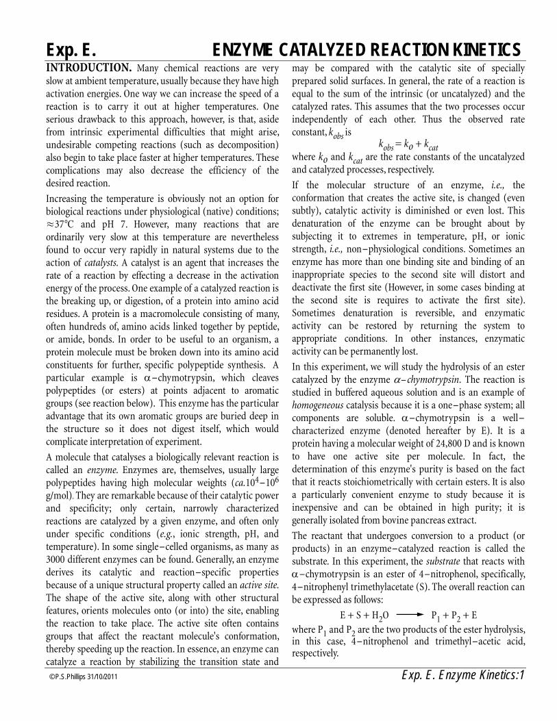
© P.S.Phillips 31/10/2011 Exp. E. Enzyme Kinetics:1
Exp. E. ENZYME CATALYZED REACTION KINETICS INTRODUCTION. Many chemical reactions are very slow at ambient temperature, usually because they have high activation energies. One way we can increase the speed of a reaction is to carry it out at higher temperatures. One serious drawback to this approach, however, is that, aside from intrinsic experimental difficulties that might arise, undesirable competing reactions (such as decomposition) also begin to take place faster at higher temperatures. These complications may also decrease the efficiency of the desired reaction.
Increasing the temperature is obviously not an option for biological reactions under physiological (native) conditions; ~37C and pH 7. However, many reactions that are ordinarily very slow at this temperature are nevertheless found to occur very rapidly in natural systems due to the action of catalysts. A catalyst is an agent that increases the rate of a reaction by effecting a decrease in the activation energy of the process. One example of a catalyzed reaction is the breaking up, or digestion, of a protein into amino acid residues. A protein is a macromolecule consisting of many, often hundreds of, amino acids linked together by peptide, or amide, bonds. In order to be useful to an organism, a protein molecule must be broken down into its amino acid constituents for further, specific polypeptide synthesis. A particular example is α-chymotrypsin, which cleaves polypeptides (or esters) at points adjacent to aromatic groups (see reaction below). This enzyme has the particular advantage that its own aromatic groups are buried deep in the structure so it does not digest itself, which would complicate interpretation of experiment.
A molecule that catalyses a biologically relevant reaction is called an enzyme. Enzymes are, themselves, usually large polypeptides having high molecular weights (ca.104-106 g/mol). They are remarkable because of their catalytic power and specificity; only certain, narrowly characterized reactions are catalyzed by a given enzyme, and often only under specific conditions (e.g., ionic strength, pH, and temperature). In some single-celled organisms, as many as 3000 different enzymes can be found. Generally, an enzyme derives its catalytic and reaction-specific properties because of a unique structural property called an active site. The shape of the active site, along with other structural features, orients molecules onto (or into) the site, enabling the reaction to take place. The active site often contains groups that affect the reactant molecule's conformation, thereby speeding up the reaction. In essence, an enzyme can catalyze a reaction by stabilizing the transition state and
may be compared with the catalytic site of specially prepared solid surfaces. In general, the rate of a reaction is equal to the sum of the intrinsic (or uncatalyzed) and the catalyzed rates. This assumes that the two processes occur independently of each other. Thus the observed rate constant, kobs is
kobs = ko + kcat where ko and kcat are the rate constants of the uncatalyzed and catalyzed processes, respectively.
If the molecular structure of an enzyme, i.e., the conformation that creates the active site, is changed (even subtly), catalytic activity is diminished or even lost. This denaturation of the enzyme can be brought about by subjecting it to extremes in temperature, pH, or ionic strength, i.e., non-physiological conditions. Sometimes an enzyme has more than one binding site and binding of an inappropriate species to the second site will distort and deactivate the first site (However, in some cases binding at the second site is requires to activate the first site). Sometimes denaturation is reversible, and enzymatic activity can be restored by returning the system to appropriate conditions. In other instances, enzymatic activity can be permanently lost.
In this experiment, we will study the hydrolysis of an ester catalyzed by the enzyme α-chymotrypsin. The reaction is studied in buffered aqueous solution and is an example of homogeneous catalysis because it is a one-phase system; all components are soluble. α-chymotrypsin is a well-characterized enzyme (denoted hereafter by E). It is a protein having a molecular weight of 24,800 D and is known to have one active site per molecule. In fact, the determination of this enzyme's purity is based on the fact that it reacts stoichiometrically with certain esters. It is also a particularly convenient enzyme to study because it is inexpensive and can be obtained in high purity; it is generally isolated from bovine pancreas extract.
The reactant that undergoes conversion to a product (or products) in an enzyme-catalyzed reaction is called the substrate. In this experiment, the substrate that reacts with α-chymotrypsin is an ester of 4-nitrophenol, specifically, 4-nitrophenyl trimethylacetate (S). The overall reaction can be expressed as follows:
E + S + H2O [ P1 + P2 + E where P1 and P2 are the two products of the ester hydrolysis, in this case, 4-nitrophenol and trimethyl-acetic acid, respectively.

Exp. E. Enzyme Kinetics:2 © P.S.Phillips 31/10/2011
Because the reaction will be carried out at a pH 8.5, both products exist in their conjugate base forms, trimethylacetate ion and 4-nitrophenoxide ion. In principle, any ester can be used to study α-chymotrypsin catalyzed hydrolysis. By using 4-nitrophenyl trimethylacetate, however, we exploit the facts that a) the bulky alkyl group slows the reaction down to a convenient time scale for simple real-time analysis, and b) the aromatic product absorbs visible light (it has a yellow appearance). The latter property allows the course of reaction to be followed spectrophotometrically. All other species involved in this reaction are colorless.
The kinetics of this reaction are particularly interesting because when the enzyme and substrate are combined, there is an initial "burst" of nitrophenol (P1 formation, which is then followed by a gradual increase in P2 concentration. In an attempt to explain this behavior, we really need to consider several mechanisms of enzyme kinetics.
Mechanism I. The simplest scheme (the so called Michaelis-Menten mechanism) involves the reversible binding of the enzyme to the substrate, followed by the dissociation of this complex to form product:
E + S ES P + E-1
1 2
k
k k] [
This is a three-parameter mechanism (rate constants k1, k-
1, and k2). Because we intend to follow the time evolution of product, the relevant differential equation is
d
dtk
[P]= 2[ES] (1)
We must obtain a relationship between the measurable quantity, [P], and [ES]. To do this, we first write the material balance for enzyme, i.e.,
[E] =[E] + [ES]o (2)
where [E]o is the total (or bulk) enzyme molarity. Equation (2) states that the enzyme must be present either in its free form, E, or in its substrate-bound form, ES. Notice that [E]o is a measurable (and controllable) quantity.
Next, we make the assumption that the dissociation of the enzyme-substrate complex into free enzyme and unchanged substrate is faster than the reaction to form product (and enzyme). This is equivalent to saying that
k1>>k2..The consequence of this assumption is that the concentration of enzyme-substrate complex can be approximated by the equilibrium expression
[ES] ~ [E][S]/K (3)
Where K is the equilibrium constant defined for the dissociation reaction of the ES complex, ES]E + S; i.e., K = k-1/ k1. (K is often written as Km). By combining equations (2) and (3), we can express the concentration of complex as
[ES][E]
/[S]o≈
+( )1 K (4)
Finally, we exploit a common experimental simplification, namely, that of the initial rate approximation. This condition, which is often used in kinetic studies means that the substrate concentration is nearly constant for short reaction times, i.e., as long as the reaction only proceeds to a small degree of conversion. With this restriction, equation (4) becomes
[ES][E]
/[S]o
o≈
+( )1 K (5)
which means enzyme-substrate complex concentration is constant. Incorporating this result in equation (1) allows us to express the time dependence of [P] by using the boundary condition that at t=0, [P]=0
2 o
o
d[P] [E]rate of production of P,
d (1 /[S] )
k
t K≈
+ (6)
This result predicts that the product concentration initially rises linearly (when [S]~[S]o) with time and the reaction velocity is constant and thus is zero order. Catalyzed reactions often exhibit zero-order characteristics at the start of the reaction.
The rate of production of P is, of course, the velocity of the reaction, v. The maximum reaction velocity, vmax is thus given by vmax=k2[E]0 (i.e. when [S]o is large). Eqn.6 is often written as
vv
K=
+max
( )1 /[S] (7)
From which it is clear that a plot of 1/v vs. [S] will be linear with slope K/vmax, intercept (on the y-axis) of 1/vmax and intercept (on the x-axis) of –1/K. Such linearised plots are called Lineweaver-Burk plots. (Note that it not only took four biologists to achieve this simple result, but they also had the audacity to confuse everything by naming the equations after themselves).
Inhibition. Some chemicals reduce or destroy (inhibit) the catalytic activity of an enzyme (without actually destroying

© P.S.Phillips 31/10/2011 Exp. E. Enzyme Kinetics:3
the enzyme). This occurs by two mechanisms i) competitive inhibition ii) non-competitive inhibition: Competitive inhibition occurs because enzymes are usually specific to molecular shape, not the molecule itself. The result of this is that any molecule, of similar shape to the substrate, can occupy the active site and prevent it from reacting with the substrate. Non-competitive inhibition occurs when a molecule binds to the enzyme site at some position other than the active site, but results in the active site becoming distorted thus reducing it’s efficiency.
Inhibition can be readily incorporated into the mechanism above as follows: We will deal with competitive inhibition first. Firstly we modify the mass balance equation (2) to account for the fact that some of the enzyme is bound by the inhibitor [I],
[E] =[E] + [ES] + [EI]o (8)
Next we recognize that EI will be in equilibrium with E and I, i.e.
EI E + I ] with equilibrium constant
[E][I]/[EI]IK = (9)
we then proceed as before making use of (7) and (8) and we get
d[P]
d
k [S][E]2 o
t K KI≈
+ +[S] ( [I]/ )1 (10)
or, in more traditional notation
vv
K KI=
[S]max
[S] ( [I]/ )+ +1 (11)
In this case the Lineweaver-Burk plot will yield a slope and x-axis intercept that depends on the inhibitor concentration, but the y-axis intercept will be 1/vmax, independent of inhibitor concentration (why?).
The case for non-competitive inhibition is developed as above. However, we have one further species to consider, IES. That is the species where the inhibitor is bound to the enzyme-substrate complex. Once again we modify the material balance equation and introduce a new equilibrium constant ′KI for the dissociation of the complex IES to IE and S. If we (reasonably) assume that the binding of the inhibitor to the enzyme is unaffected by the presence of the substrate on the enzyme so that KI= ′KI then we get
vv
K KI=
[S]max
([S] )( [I]/ )+ +1 (12)
In this case the Lineweaver-Burk plot will yield a slope and x-axis intercept that depends on the inhibitor
concentration, but the y-axis intercept will be –1/K. The plots for the three cases are shown in figure 1 overleaf.
As we mentioned earlier, the time dependence of the 4-nitrophenoxide ion concentration in the α-chymotrypsin-catalyzed hydrolysis of the ester precursor is not linear, as predicted in equation (1); hence, Mechanism I cannot be acceptable and must be modified.
Modification of Mechanism I. We will now consider a refinement of Mechanism I in which the pre-equilibrium assumption, eq.(3), is relaxed, and see whether this modification brings the predicted rate law into conformity with the observed one. We will retain, however, the isolation condition assumption, [S]o>[E]o. We proceed by writing the differential equation for the formation of complex,
1 -1 2[ES]
[E][S]- [ES]- [ES]d
k k kdt
= (13)
After using equation (2) and replacing [S] by [S]o, we obtain, after combining terms,
1 o o -1 2 1 o[ES]
[E] [S] -( + + [S] )[ES]d
k k k kdt
= (14)
Using the definitions
1 o o[E] [S]X k= and -1 2 1 o+ + [S]Y k k k=
and integrating equation (14) with [ES]=0 at t=0, provides the time dependence
[ES]
lnX Y
YtX
æ ö- ÷ç =-÷ç ÷çè ø (15)
or more explicitly,
[ES( )] (1 exp( ))X
t YtY
æ ö÷ç= - -÷ç ÷çè ø (16)
The rate equation for product formation is obtained by combining equations (1) and (15). We get for the reaction velocity,
( )2[P]1 exp( )
d k XYt
dt Y
æ ö÷ç= - -÷ç ÷çè ø (17)
and after integrating this equation and simplifying the result, we see that the time dependence of product is
( )2 22
[P( )] 1 exp( )k X k X
t t YtY Y
æ öæ ö ÷÷ çç= - - -÷÷ çç ÷÷ç ÷çè ø è ø (18)
Predictably, perhaps, this result is more complex than that in equation (6). Inspection of equation (18) reveals that after a certain time, the second term becomes constant (-k2/Y2), and the product formation, [P] vs. t, is (again) zero order,
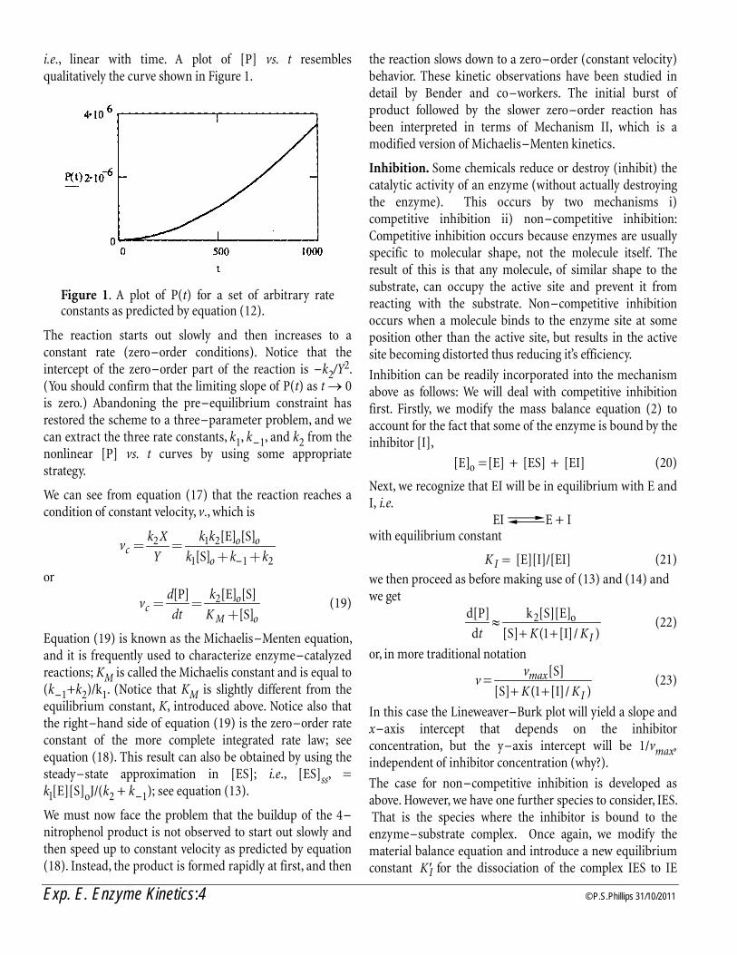
Exp. E. Enzyme Kinetics:4 © P.S.Phillips 31/10/2011
i.e., linear with time. A plot of [P] vs. t resembles qualitatively the curve shown in Figure 1.
Figure 1. A plot of P(t) for a set of arbitrary rate constants as predicted by equation (12).
The reaction starts out slowly and then increases to a constant rate (zero-order conditions). Notice that the intercept of the zero-order part of the reaction is -k2/Y2. (You should confirm that the limiting slope of P(t) as t → 0 is zero.) Abandoning the pre-equilibrium constraint has restored the scheme to a three-parameter problem, and we can extract the three rate constants, k1, k-1, and k2 from the nonlinear [P] vs. t curves by using some appropriate strategy.
We can see from equation (17) that the reaction reaches a condition of constant velocity, v., which is
2 1 2
1 -1 2
[E] [S]
[S]o o
co
k X k kv
Y k k k= =
+ +
or
2[P] [E] [S]
[S]o
cM o
d kv
dt K= =
+ (19)
Equation (19) is known as the Michaelis-Menten equation, and it is frequently used to characterize enzyme-catalyzed reactions; KM is called the Michaelis constant and is equal to (k-1+k2)/k1. (Notice that KM is slightly different from the equilibrium constant, K, introduced above. Notice also that the right-hand side of equation (19) is the zero-order rate constant of the more complete integrated rate law; see equation (18). This result can also be obtained by using the steady-state approximation in [ES]; i.e., [ES]ss, = kl[E][S]oJ/(k2 + k-1); see equation (13).
We must now face the problem that the buildup of the 4-nitrophenol product is not observed to start out slowly and then speed up to constant velocity as predicted by equation (18). Instead, the product is formed rapidly at first, and then
the reaction slows down to a zero-order (constant velocity) behavior. These kinetic observations have been studied in detail by Bender and co-workers. The initial burst of product followed by the slower zero-order reaction has been interpreted in terms of Mechanism II, which is a modified version of Michaelis-Menten kinetics.
Inhibition. Some chemicals reduce or destroy (inhibit) the catalytic activity of an enzyme (without actually destroying the enzyme). This occurs by two mechanisms i) competitive inhibition ii) non-competitive inhibition: Competitive inhibition occurs because enzymes are usually specific to molecular shape, not the molecule itself. The result of this is that any molecule, of similar shape to the substrate, can occupy the active site and prevent it from reacting with the substrate. Non-competitive inhibition occurs when a molecule binds to the enzyme site at some position other than the active site, but results in the active site becoming distorted thus reducing it’s efficiency.
Inhibition can be readily incorporated into the mechanism above as follows: We will deal with competitive inhibition first. Firstly, we modify the mass balance equation (2) to account for the fact that some of the enzyme is bound by the inhibitor [I],
[E] =[E] + [ES] + [EI]o (20)
Next, we recognize that EI will be in equilibrium with E and I, i.e.
EI E + I ] with equilibrium constant
[E][I]/[EI]IK = (21)
we then proceed as before making use of (13) and (14) and we get
d[P]
d
k [S][E]2 o
t K KI≈
+ +[S] ( [I]/ )1 (22)
or, in more traditional notation
vv
K KI=
[S]max
[S] ( [I]/ )+ +1 (23)
In this case the Lineweaver-Burk plot will yield a slope and x-axis intercept that depends on the inhibitor concentration, but the y-axis intercept will be 1/vmax, independent of inhibitor concentration (why?).
The case for non-competitive inhibition is developed as above. However, we have one further species to consider, IES. That is the species where the inhibitor is bound to the enzyme-substrate complex. Once again, we modify the material balance equation and introduce a new equilibrium constant ′KI for the dissociation of the complex IES to IE

© P.S.Phillips 31/10/2011 Exp. E. Enzyme Kinetics:5
and S. If we (reasonably) assume that the binding of the inhibitor to the enzyme is unaffected by the presence of the substrate on the enzyme so that KI= ′KI then we get
vv
K KI=
[S]max
([S] )( [I]/ )+ +1 (24)
In this case, the Lineweaver-Burk plot will yield a slope and x-axis intercept that depends on the inhibitor concentration, but the y-axis intercept will be –1/K. The plots for the three cases are shown in figure 2 overleaf.
Mechanism II The basic assumptions underlying this mechanism are: 1. The ester and enzyme form a reversible complex that is in a rapid pre-equilibrium. 2. The ester binds to the active site of the enzyme causing the acylation of the enzyme (attachment of the RCO- group) and the release of 4-nitrophenoxide ion (P1). 3. The acylenzyme is then deacylated, releasing the trimethylacetate ion, P2, thereby restoring the active enzyme, which can catalyze the hydrolysis of another ester molecule. The following reaction scheme portrays this mechanism:
The mechanism can be expressed kinetically, as follows:
1
-1
E + S ES k
k ] reversible enzyme -substrate binding
2
1ES P + AEk
[ enzyme acylation
3
2AES P + Ek
[ enzyme deacylation
where AE is the acylenzyme (see the scheme). Notice that although P1, which is monitored in this experiment, is released before P2 is produced, the last step is nevertheless important kinetically because it produces the active enzyme, which can then "recycle" and thus react with another substrate.
The scheme described by Mechanism II now contains four parameters, k1 k-1, k2, and k3, but by invoking the pre-equilibrium condition, we can reduce the number of unknowns to three, because K= k-1/k1,. We again assume that [S]o > [E]o. Our objective, as before, is to obtain the time dependence of the observed product, P,. We start by writing the differential rate laws for [P1] and [ES]
12
[P ][ES]
dk
dt= (25)
and
1 -1 2[ES]
[ ][S] [ES] [ES]d
k E k kdt
= - - (26)
The mass balance equation for enzyme gives
[E]o = [E] +[ES] + [AE] (27)
In addition, the equilibrium assumption gives us
-1 o
1
[E][S] [E][S]
[ES] [ES]
kK
kº = » (28)
By combining equations (27) and (28), we can express [ES] in terms of [AE]
o
o
[E] -[AE][ES]
1+ /[S]K= (29)
We will now have to determine the time dependence of the acylenzyme, AE. This step is necessary in order express ES as a function of time. We will then use that result in equation (25) to arrive at the desired result. We proceed by writing the rate law for [AE]:
2 2[AE]
[ES] [AE]d
k kdt
= - (30)
and using [ES] from equation (29) to obtain, after collecting terms,
2 o 23
o o
[AE] [E][AE]
1+ /[S] 1+ /[S]
d k kk
dt K K
æ ö÷ç ÷= - +ç ÷ç ÷çè ø (31)
For convenience, we use the definitions
2 o 23
o o
[E]
1+ /[S] 1+ /[S]
k kA B k
K K= = + (32)
The solution of the differential equation d[AE]/dt = A-B[AE] with the boundary condition t = 0, [AE] = 0 is
[AE]ln
A BBt
A
æ ö- ÷ç =-÷ç ÷çè ø
or, explicitly,
[AE] (1 exp( ))A
BtB
= - - (33)

Exp. E. Enzyme Kinetics:6 © P.S.Phillips 31/10/2011
After substituting this expression for [AE] in equation (29), we get, after rearranging,
o
o o
[E] / /[ES] exp( )
1+ /[S] 1+ /[S]
A B A BBt
K K
-= + - (34)
Notice that according to eq.(34) the ES adduct has a finite concentration at t=0; this physically unreasonable result is a consequence of the pre-equilibrium assumption. Eq.(34) clears the way to expressing the needed time dependence of P,; by combining equations (34) and (25), we find,
1 o 22
o o
[P ] [E] / ( / )exp( )
1+ /[S] 1+ /[S]
d A B k A Bk Bt
dt K K
æ ö æ ö- ÷ ÷ç ç÷ ÷= + -ç ç÷ ÷ç ç÷ ÷ç çè ø è ø (35)
We can integrate this equation to obtain the direct time dependence of P1. The result appears in the form
( )1( ) ( ) 1 exp( )P t X t Y Bt= + - - (36)
in which B is defined in (32), and X and Y are expressions that contain rate constants and initial enzyme and substrate concentrations, i.e.,
o2
o
[E] /
1+ /[S]
A BX k
K
æ ö- ÷ç ÷= ç ÷ç ÷çè ø (37)
22
o(1+ /[S] )
k AY
B K= (38)
Eq.(36) is sketched in Figure 2. This P vs. t curve now conforms to the observation of an initial burst of product followed by a constant rate of product formation. Notice that according to eq.(36), the approach to zero-order kinetics
takes place exponentially (with an apparent rate constant B). Thus for a given set of [E]o and [S]o values, the analysis of curves like that shown in Figure 2 provides three pieces of information, X, Y, and B. We now face the challenge of extracting the three specific system parameters, K, k2, and k3, from this information. In principle, all we need to do is evaluate X, Y, and B from one kinetic experiment of [P1] vs. t, and to solve equations (37) and (38), with the definitions in (32), to obtain K, k2, and k3. In practice, this is not a practical way to proceed because the transformations are too mathematically obtuse. In concept, and we would have to measure X, Y and B at different [E]o and [S]o values, and to use appropriate mathematical transformations of equations (37-39) to extract the rate parameters. Some simplified approaches are presented next.
Figure 3. Plot of P(t) eq.(36) for an arbitrary set of rate constants.
At this point, remember that the substrate in this reaction undergoes spontaneous, or uncatalyzed, hydrolysis in
Figure 2. From left to right. Lineweaver-Burk plots a reaction with no inhibitor at various concentrations of a competitive (middle) and non-competitive inhibitor (right)

© P.S.Phillips 31/10/2011 Exp. E. Enzyme Kinetics:7
parallel with the enzyme-catalyzed reaction. Each process forms the same species, P1, that is followed spectrometrically. Thus, hence you must subtract the uncatalyzed "blank" kinetic run from the experimentally acquired data file to obtain the actual time dependence of the catalyzed reaction that is modeled in eq. (36).
In the case of the α-chymotrypsin-4-nitrophenyl trimethylacetate system studied in this experiment, one important point is that the enzyme used is not pure α-chymotrypsin; the material contains some impurities (including water of hydration). Thus, its bulk concentration is not equal to the enzyme molarity. Instead, we may write
o act o bulk[E] [E]p=
where o act[E] is the initial concentration of active (i.e., pure) enzyme, and o bulk[E] is the initial bulk concentration of the enzyme (i.e., as weighed out in the experiment), and p is the purity factor of the raw enzyme; thus the activity of the enzyme (expressed as a percent) is 100p. We will show next how it is possible to estimate p from the kinetic data. We will assume that values of X, Y, and B have been obtained from a kinetic run at known o bulk[E] and [S]o. Preferably these values have been determined from several different runs at fixed o bulk[E] and various initial substrate concentrations, [S]o. First, we consider X (eq.(37)). With a little work, we may recast X to read
2 3o act o
2 3
3o
2 3
[E] [S]
[S]
k k
k kX
kK
k k
+=
++
(39)
(We emphasize that the enzyme concentration corresponds to the active enzyme.) The reason we present equation (39) is that it has the form of a Michaelis-Menten, (19). Notice that X has units of M s-1, i.e., a rate. This point is clarified by rewriting (39) as
o act o
o
[E] [S]
[S]cat
M
kX
K=
+ (40)
in which kcat = k2k3/(k2 + k3) and KM, an apparent Michaelis constant, is k3K/(k2 + k3). In its recast form, we can conveniently transform X to the linear equation
o act o act o
1 1
[E] [E] [S]M
cat cat
K
X k k= + (41)
which we may use to obtain kcat and KM by plotting 1/X vs. 1/[S]o (if we know o act[E] ). Alternatively, we may apply a nonlinear regression analysis of (X[S]o) data to equation (41). We may invoke an approximation that is justified by
prior knowledge of the α-chymotrypsin-p-nitrophenyl trimethylacetate system, namely, that we can choose [S]o values such that [S]o> KM. With this inequality, equation (41) simplifies to
X = kcat[E]o act (42)
and we can obtain kcat, as long as we know o act[E] . But as we pointed out above, the experimental [E]o is the bulk concentration of enzyme. We need to know p, the actual enzyme activity, in order to obtain o act[E] . To obtain p, we examine the kinetic parameter Y, which we may recast as
22
2 3o act
o
[E]1
[S]M
k
k kY
K
æ ö÷ç ÷ç ÷ç + ÷ç ÷= ç ÷÷ç ÷ç ÷+ç ÷ç ÷çè ø
(43)
Again, using prior knowledge of the system studied here, we add to the inequality [S]o>KM the approximation that k2 > k3. These statements greatly simplify equation (43), so that o act[E]Y » (44)
and we may obtain o act[E] directly from the rate parameter Y. Once we know o act[E] equation (42) immediately furnishes a value of kcat, which, considering the inequality k2>k3, is approximately equal to k3, the enzyme deacylation rate constant.
If the inequalities are not justified, we can, with some effort, transform equation (43) to read
2 3 2 3
2 o act 2 o act
1 1 ( )
[E] [E]Mk k K k k
kY k
æ ö+ +÷ç ÷= +ç ÷ç ÷çè ø (45)
and we can use a plot of o1/ . 1/[S]Y vs to obtain KM and k2/(k2 + k3).
Finally, we may recast B, see (32), into a more convenient form (using the approximation that k3K < (k2 + k3)[S]o; i.e., KM< [S]o ):
2 3 2 3 o
1 1 1
[S]
K
B k k k k
æ ö÷ç ÷= +ç ÷ç ÷ç+ +è ø (46)
in which a double-reciprocal plot of B and [S]o will yield K and k2 + k3. If B is not determined at different substrate concentrations, the approximations [S]o<K and k2>k3 may be made, in which case,
2 o[S]kB
K= (47)

Exp. E. Enzyme Kinetics:8 © P.S.Phillips 31/10/2011
PROCEDURE. Solutions Needed. Prepare the following solutions. 1. Solution #1. Prepare (or obtain) about 60mL of a TRIS buffer with pH = 8.5 (0.01 M). You will use this solution as the reaction medium and also as a solvent blank. 2. Solution #2. Prepare a 3.4 x 10⁻³ M solution of the substrate, 4-nitrophenyl trimethylacetate, in acetonitrile. About 10mL is sufficient for one experiment, although 25mL may be more convenient to prepare. (Use appropriate caution when using acetonitrile. Wear protective gloves and work in a fume hood.) 3. Solution #3. Obtain α-chymotrypsin solution (about 50mg of α-chymotrypsin in 1.0mL of the pH 4.6 acetate buffer). You will use this directly in the kinetic run. 4. Solution #4. Make up 5 or 10mL of a 2.8 × 10⁻⁵M solution of 4-nitrophenol solution in the TRIS buffer. You will use this solution to determine the molar absorptivity of the product, P1. Note that since the pKa of 4-nitrophenol is about 7.0, the predominant species in the pH 8.5 TRIS buffer is the 4-nitrophenoxide ion. 5. Solution #5. Make up 100mL of a 3.0x10⁻³M solution of Malthion (MW=330) in acetone from the stock solution of commercial Malthion (1.5M). Note that Malthion smells and, more importantly, inhibits the enzyme acetylo-cholinase; the enzyme that plays a key role in nerve signal transmission. This is a characteristic of nerve gases and many modern pesticides; breathing them in or splashing them on the skin results in central nervous system failure (a.k.a. death). Be sure to use gloves, make up the solutions in the fume hood and keep them stoppered when not in use.
Determination of the Molar Absorptivity of 4-Nitrophenol. Set the spectrophotometer wavelength to 400 nm, the position at which the hydrolysis product, P1 is measured. Use two matched, 1cm spectrophotometer cells. Preferably these should be constructed of fused silica, but Pyrex cells are acceptable at this wavelength. Add TRIS buffer to both cells, place them in the spectrophotometer cavity, and zero the instrument. Remove the sample cell and rinse and fill it with the 2.8 × 10⁻⁵M 4-nitrophenol solution in the sample cell (solution #4). Replace the cell in the spectrophotometer, and record the absorbance.
Determination of the Spontaneous Hydrolysis Rate of the Substrate. To determine the rate constant of the uncatalyzed (i.e., spontaneous) hydrolysis of 4-nitrophenyl trimethyl-acetate, fill a clean sample cell with precisely 3mL of TRIS buffer. Add 100uL of the 3.4 x 10⁻³M 4-nitrophenyl trimethylacetate/acetonitrile solution (solution #2). Stopper (or cap) the cell, invert it a few times, and place
it in the spectrophotometer cavity (make sure a reference cell containing TRIS buffer is in place), and record the absorbance at 400nm for at least 2 min., every 5s. In this and the enzyme kinetic runs, thermostat the cell if possible. Record the temperature in your notebook. Save the data file in ASCII format. Do not keep this run on the screen, clear it off the instrument.
Run the Reaction. Add 3.0mL of TRIS buffer to the reaction cell (use a pipetter). Place it in the spectrophotometer cavity and zero the instrument at 400nm. Make sure the reference cell contains the same buffer solution. Now, add between 10 and 100µL of the substrate stock solution (solution #2) depending on which sample (samples 1-5) you intend to run (see table 1, use a GC syringe to measure the solutions). Mix thoroughly.
Sample No. Substrate
volume (µL) Inhibitor
volume (µL) Reference 0 0
1 20 0 2 25 0 3 30 0 4 50 0 5 100 0 6 20 40 7 25 40 8 30 40
9 50 40 10 100 40
Table 1. Solutions to run. All samples are made up in 3.0mL of TRIS buffer.
Next add the enzyme to the reaction solution. Use 40µL of the enzyme stock solution (solution #3 above). There are several possible techniques for introducing the enzyme: a) Directly inject the appropriate volume of the enzyme stock solution into the reaction cell; quickly cap the cell, invert it several times (do not shake), place it in the spectrophotometer, and immediately begin data acquisition (remember you want the initial rate). b) Alternatively, you can deposit the enzyme solution onto the tip of a clean, small stirring rod that you then immerse in the cell and use to stir the reaction mixture. Place the cell in the spectrophotometer and begin data acquisition. (Experiment with this technique beforehand; it may be useful to wet the tip of the stirring rod sparingly with buffer solvent.) Collection time should be about 2 min. with data points every 5s (we are only interested in the initial rate). Save the

© P.S.Phillips 31/10/2011 Exp. E. Enzyme Kinetics:9
data file in ASCII format. Repeat until all five solutions have been run. Once you have the data saved, clear it, do not accumulate the inhibited runs on top of it. You can run out of memory if you do (the spectrometer can save 10 spectra only).
Testing an inhibitor. Repeat the runs above, but in addition add some Malathion inhibitor (solution #6) as indicated in table 1 (samples 6-10). Again, remember to save the data file in ASCII format.
Data Analysis. Import the data files to Excel. You will also need a program that is capable of performing nonlinear regression analysis on user-defined functions (Origin). We furthermore assume that each data file (including the spontaneous substrate hydrolysis blank) has the same time interval between data points, and the total acquisition times are nominally equal.
Subtract the spontaneous hydrolysis blank from each of the kinetic runs. However, before doing this, multiply the absorbance values of the blank file by an appropriate factor that reflects the different substrate concentrations used. For example, if you used 100µL in the blank and 80µL for the kinetic run, multiply the absorbances of the blank file by 0.8 before subtracting them from the kinetic data file. (This assumes that the spontaneous hydrolysis constant, ko, is independent of concentration.) Then, convert absorbance to concentration using the molar absorptivity of the product (4-nitrophenoxide ion) determined in this experiment.
Perform a nonlinear regression analysis (you’ll need help with this - using Origin’s non-linear fitting routines - you can download a demo version off the net) on the acquired P1 vs. t data sets according to equation (36), and thus obtain in each case X, Y, and B. From equation (42), obtain kcat [E]o
act and KM by regressing 1/X vs. 1/[S]o. Also, find the purity factor, p, from the known bulk concentration of enzyme.
From equation (47) determine the quotient k2/K. If you have obtained X, Y, and B at several substrate concentrations, use equation (41) to find kcat and KM. Compare these values with those obtained from equation (45). Finally, determine k2 + k3 and K from the double-reciprocal plot displayed in equation (46).
Test the inequalities used in some of the derivations, namely, [S]o > KM and k2 > k3.
QUESTIONS. 1) The mechanism is more complex than the simple Michaelis-Menten one so we cannot determine if the Malathion is competitive or non-competitive using a
Lineweaver-Burk plot. However, Malthion will affect the enzyme the same way so it should be possible to deduce the effect on the kinetic runs and consequently (with luck) which it actually is. 2) You were told to invert the UV-cell several times to mix the enzyme, not to shake it. Explain why. (Assume the cell is properly capped so that spillage is not a problem). 3) The spacing of the substrate volume added is not uniform. Why did we do that ? REFERENCES. R. A. Alberty and R. J. Silbey, Physical Chemistry, 2nd ed., pp. 730-736, Wiley (New York), 1997. P. W. Atkins, Physical Chemistry, 5th ed., pp. 890-891, W. H. Freeman (New York), 1994. P. W. Atkins, The Elements of Physical Chemistry, 1st ed. pp270-277, Oxford (Oxford), 1992. M. L. Bender, F. J. Kezdy and F. C. Wedler, J. Chem. Educ., 44:84 (1967). M. L. Bender and F. J. Kezdy, J. Amer. Chem. Soc., 86:3704 (1964). I. N. Levine, Physical Chemistry, 4th ed., pp. 542-545, McGraw-Hill (New York), 1995. J. B. Milslien and T. H. Fyfe, Biochemistry, 8:23 (1969). J. H. Noggle, Physical Chemistry, 3rd ed., pp. 576-582, Harper Collins (New York), 1996. T. W. G. Solomons, Organic Chemistry, 5th ed., pp. 1181-1184, Wiley (New York) 1996. L. Stryer, Biochemistry, 4th ed., pp. 222-227, W. H. Freeman (New York) 1995. I. Tinoco, Jr., K. Sauer, and J. C. Wang, Physical Chemistry: Principles and Applications in Biological Sciences, pp. 418-441, Prentice Hall (Englewood Cliffs, N. J.), 1995

Exp. E. Enzyme Kinetics:10 © P.S.Phillips 31/10/2011
NOTES

© P.S.Phillips October 31, 2011 EXPERIMENT G:1
Suite G. THERMODYNAMICS OF GLYCINEINTRODUCTION. Want to know the heat of solution of glycine? You just pickup Lange or the CRC and look it up. However, what if you wanted to know the heat of solution of glycine in something that approximates blood plasma, then what? You will have to spend a lot of time in the literature or, you will have measure it. Here we will explore the measurement of some thermodynamic parameters for glycine, the simplest of the amino acids. The experiment should give you some insight into doing these measurements under non-standard conditions, and how to do them rigorously.
In part I, we will simply measure the two pKa values for glycine and explore some numerical tools, including programming Maple, to assist us in getting a reliable value. In part 2 we explore the enthalpy of proton transfer for glycine and pay attention to activity effects. If part 3 we will find the enthalpy of formation of glycine and pay particular attention to error analysis.
Part 1. ACID BASE TITRIMETRY INTRODUCTION. This is a simple pH/conductiometry titration. Glycine has to apK s so the experiment has to be modified accordingly.
THEORY. The theory of strong acids and bases is sufficiently simple to need no further elaboration here. However, the theory for titration of weak acids is messy and is developed in appendix I, from which we can show that the concentration of hydrogen ion during the titration of a weak acid with a strong base is;
[H+]3+α[H+]2-β [H+]-KaKw = 0 (1.1)
where Vao is the initial volume of the analyte, cb
o is the initial concentration of analyte, Vb is the volume of titrant added, cb
o is the concentration of titrant and
(1 ) =
1 1
o oa a a
a wc f c K f
K Krf rf
a b-
= ) )) )
where r c cao
bo= / , and the fraction of analyte titrated, f, is
f V c V cb bo
ao
ao= / . These equations enable us to extract Ka
using the whole titration curve rather than just the one ill-defined end-point.
PROCEDURE. This is a simple pH titration. First, you need to calibrate the pH meter, using the provided standard buffers (pH 4.00, pH 7.00 and pH 9.00 or 10.00). You will be shown how to do this. Make sure you don’t get cross
contamination between the standard buffers, and swish the electrode around. Remember to let the reading stabilize.
Glycine has two pKa’s so we are going to start with a solution of glycine hydrochloride (you make). You will be provided with your titrant; accurately made KOH solution (exact value on the bottle).
We will titrate glycine hydrochloride with KOH over a pH range of about 2 to 13, and record the pH as a function of volume of KOH added. You will need to do a rough titration first to get the two approximate end-points. This will give you the two pKa values for glycine.
Proceed as follows. Makeup 100 mL of 0.1M glycine HCl (it need not be exactly 0.1, but you should know what it is accurately.) Take a 25.0 mL aliquot and adjust the pH < 2.0, if necessary, with a few drops of the supplied standard 0.1M HCl (corrosive!). Titrate this solution with the 0.25M KOH solution provided
Collect data about every 0.5 mL except near the end-point where the pH changes rapidly. At that point change to 0.1ml increments. The increments can be approximate but you must know what the increment is to within 0.005mL, or whatever you can be read the burette to. You may have to let the pH meter stabilize between readings.
Repeat the titration using 0.1 mL increments either side of the first end point and about 0.2mL around the second endpoint. You will need to plot your first data set to establish what “around the endpoint” means.
Ask the instructor if they want you to repeat the experiment with glutamic acid. In that case you make need to run to pH 8, or do an intermediate titration with 0.2M or 0.5M acid. Discuss your observations in your report.
CALCULATIONS. Do the following calculations for both the titrations.
1) Determine the end-point and hence the pKa‘s of both the acids directly from a plot of pH vs. VNaOH.
2) Determine the pKa of both the acids from a plot of dpH/dV vs. VNaOH. That is, setup Excel to do a simple derivative using 1 1/ ( ) / ( )i i i idy dx y y x x) )» - - . You may have to drop the first few points of the amino acid titration. Typical results are shown in figure 1.1 below.
3) Repeat the two plots of the titration curve using CurveFit (if provided by the instructor) with the cubic spline (with and without tension) and Akima spline. One method works better than the other.

EXPERIMENT G:2 © P.S.Phillips October 31, 2011
4) Fit the titration curve to a cubic (in the vicinity of each pKa and get α and β in (1.1) and hence the pKa’s.
5) If you were asked to do a titration using conductivity, repeat the process with the conductivity data using the method of broken lines and the derivative method.
Figure 1.1 Typical titration curve and the differential. The weaker the acid (or base) the less well defined the inflection point becomes.
5) Get the pKa using a Gran plot. That is, plot [H+]VNaOH vs. VNaOH. The slope of the line is –Ka and the x-axis intercept is the equivalence point. Compare those values with those obtained by the other methods. You may want to use the robust LSF to fit the data (CurveFit again). At the very least, you may have to eliminate points from the plot ends before fitting. Note you cannot use this plot over the whole range: select data from around the end-points
QUESTIONS. 1) Compare your data to the literature values. Does the pKa in the 0.3M NaCl differ from water or its literature value?
2) We often talk about sharp and fuzzy to describe slope changes or breaks. The formal terms to describe lines are smoothness, monotonicity and continuity. Briefly, describe the correct descriptions for the terms and support with some math. Be sure to distinguish between the informal and formal definitions of smooth. 3) The conductivity data will go through a minimum. Explain this and the general structure of the titration curve.
Part 2. SOLUTION THERMODYNAMICS INTRODUCTION. As elegant as thermodynamics is (everything follows from the first two laws) there is no way of predicting enthalpies or entropies; they must be measured. Some simplification occurs because we measure state functions so data that are not directly measurable are accessible via what I call the cycle method (just a variation of Hess’s Law). In this experiment, we will measure the heat of protonation of an amino acid (glycine) in aqueous solution via its heat of solution and heat of reaction for solid
glycine. This lab. illustrates the complexity of such apparently simple experiments. In fact, we will have to take some short cuts and make use of literature values or we wouldn’t have time to do it all.
THEORY. Here, we are interested in the enthalpy of protonation ( protonHD of glycine, HGly) in aqueous solution, that is
H+(aq) + HGly (aq) ] H2Gly+(aq) (2.1)
This is characterized by 2apK for glycine. Note that this
reaction is not the dissociation of glycine (or the reverse), that is given by
HGly (aq) ] H+(aq) + Gly-(aq) (2.2)
and characterized by the1apK for glycine.
I have dropped the superscript “o” from the enthalpies for convenience, they do, however, refer to standard conditions.
We can obtain protonHD from the temperature dependence of the pKa . Here we will obtain it from calorimetric reaction cycles:
Reaction 1. + +
1+
2
(Gly)HGly( ) H ( ) HGly( ) H ( )
(HGly( )) H Gly (aq)
protonrx
dissolnHs aq aq aq
H aqH
D) ¾¾¾¾¾¾® )
DD
This is the dissolution of glycine in hydrochloric acid and it’s subsequent protonation. The protonation is not complete and has to be accounted for. In the presence of excess acid, there is no significant dissociation of glycine so this is ignored.
Reaction 2.
- +
(Gly) HGly( ) HGly( )
(HGly( ))
Gly ( ) H
dissocsoln
dissolnHs aq
H aqH
aq
D¾¾¾¾¾¾®
DD
)
This is simply the dissolution of glycine and it’s subsequent dissociation, normally referred to as the heat of solution. The dissociation is not complete and has to be accounted for; see later. The protonation of glycine is not significant under these circumstances and can be ignored. Note the distinction between enthalpy of solution (just adding glycine to water) and enthalpy of dissolution.
Reaction 3.
+ -2 2 3 2NH CH COOH NH CH COO
That is, dissociation to the zwitterion. It turns out that

© P.S.Phillips October 31, 2011 EXPERIMENT G:3
glycine only exists as the zwitterion in solution. This is discussed below.
By examining these schemes above you can see that to get the enthalpy of protonation ( protonHD ) one needs the enthalpy of dissolution ( dissolnHD ) and the enthalpy of dissociation ( dissocHD , see the appendix). The enthalpy of dissolution can then be obtained from reaction cycle 2:
- + proton rx1 soln dissocH H H HD = D D D
There are three problems, however: The first is that the reaction (1) is done in a 0.3M HCl solution. This is strong enough to influence the activities, and thus the reaction enthalpy. This is overcome by doing the enthalpy of solution (reaction (2.2)) in a solvent of the same ionic strength, in this case, 0.3M KCl.
The second problem is quite insidious. Neutral glycine does not exist in solution (at least only 1 in ¼ million) it exists as the zwitterion. However, since it’s always in this form no parameter relating to neutral glycine appears in the equations, so it actually doesn’t matter. However, this is not true of other amino acids where the zwitterion may not dominate.
The third problem is that glycine is not a very acidic so it does not completely dissociate in solution. We thus have to adjust for the degree of dissociation. We can get K1 for dissociation from the appendix. For n moles of glycine we have the ‘ICE’ calculation
HGly(aq)]H+(aq) + Gly- (aq)
n 0 0
n-α – α - α and
+ -
1[H ][Gly ]
[HGly]K =
from which we get 2
1 ( )0.1K
n
αα
=−
Equilibrium constants are for concentrations, not moles, so the factor of 0.1 is to correct for the 100mL solution. Hence we get the factor, 1/α, to multiply the enthalpy of dissociation by to correct for incomplete dissociation (1/α should be about 500).
BASIC PROCEDURE. The calorimeter is a Dewar flask containing a rotating sample cell and a thermocouple (see fig.1) attached to a data processing unit. A known amount of acid (about 100g) will be measured into it, the stirrer will be run continuously, and calorimetric measurements will be
made while a sample of glycine is dissolved in the acid. The temperature is recorded continuously throughout the course of the experiment. The heat change is determined by comparison with a standard run (of adding TRIS to 0.1M HCl). Since we will be using solid glycine, we have to do a third run to establish the heat of solution of the glycine.
You will be dealing with changes in temperature of less than a degree so you should be definitely trying to get better than 1% accuracy for the various individual measurements. A temperature measurement to 0.01C may look impressive to you, but it is not much good for this experiment. The thermocouple is precise to 0.001C, if correctly used. You will have to be very careful to get decent results.
CALORIMETER DISASSEMBLY/ASSEMBLY. The apparatus contains some very fragile glass bits. Be careful when handling them, you'll need a bank balance with five significant figures to repair them. If the calorimeter is assembled (see Figure 2.1), disassemble as follows: If the glass push rod is raised, push it down gently to eject the sample dish. Disengage the drive belt if on. Then gently lift the whole assembly out of the calorimeter and place it in the retort ring provided. NOTE: that the thermocouple is plugged into the back of the calorimeter so don't expect to be able to move the assembly very far without unplugging it first. Hold the glass plunger rod and pull off the Teflon sample cup while twisting it and then slide out the glass rod. Inspect the sample cell and sample dish for dirt and water. Carefully clean and dry if necessary. Now, carefully lift out the Dewar flask and clean and dry if necessary. Reverse the process (including cleaning and drying) to assemble the apparatus. If the calorimeter is already disassembled, familiarize yourself with each of the components and the order in which they fit.
Figure 2.1. Schematic of solution calorimeter.

EXPERIMENT G:4 © P.S.Phillips October 31, 2011
PROCEDURE IN CHRONOLOGICAL ORDER. This experiment goes faster if you coordinate your efforts so read all the instructions first. You may want to do a dry run first (no solutions or glycine); in particular make sure you can assemble the sample cell. First, turn on the calorimeter (switch is on rear left) to check that it's OK. The calorimeter may give a message about re-booting the RAM disk. If it does, just press the <ENTER> button, then <ENTER> again when it prompts for the date, then again when it prompts for the time.
PART I. Heat of reaction.
1. One partner should accurately (4dp) weigh 1.00+0.05 of dried glycine on an analytical balance into a stoppered weighing vial. You may want to pre-weigh the sample on a top-loading balance. The glycine has been ground and dried (and is stored in a desiccator) so minimize exposure to the air! Don't weigh out any big lumps; they won't fit in the dish. Also, prepare the standard sample (see below).
2. Meanwhile, your partner should prepare (or otherwise obtain) a 0.30M solution of hydrochloric acid. Then put about 120mL of the HCl solution into a flask and warm it to 25.5 to 26C, but no more, by running it under the hot tap. When done, weigh to 2dp. about 100g of the warm solution into the Dewar and it back into the calorimeter.
3. Carefully pour the glycine sample into the Teflon sample dish (don't spill any or get it into the center hole, if you do, start that sample again. The sample will nearly fill the dish). Place the sample dish on the bench and hold the sample cell exactly vertically above it and gently press down on the stem of the sample cell until the dish is seated in the bell (it should not take much pressure to do this; do not force it). Now slip in the glass push rod and press on it firmly so it sticks in the sample dish hole.
4. Place the assembly carefully into the Dewar and attach the stirrer belt (at the motor first). Now press *122<ENTER> (with your finger tip NOT your finger nail), you will be prompted for the DAC SPAN (DAC = digital to analog converter), press 1<ENTER> (this means that a 1C change from the offset temperature, vide infra, will produce an output of 10V). Next press *250<ENTER> then 5<ENTER>, wait for about 30 seconds then press *250<ENTER> again followed by 0<ENTER>. (This recalibrates the thermocouple). Note that this calorimeter is very sophisticated, but unforgiving, and pressing any other combination of the buttons will produce all sorts of weird results. For instance it will recalibrate itself in the middle of your runs so don't do it. Now, take a few minutes to check that the (beige) Linear chart recorder is ready. It should be
set for a chart speed of 2cm/min, a sensitivity of 5V and the attenuator must be switched to calibrate (this means that an input of 5V moves the pen 10in – the paper is cm on the x-axis and inches on the y-axis). Put in record mode and lower the pen. Make sure it is plugged into the calorimeter, and then zero the pen to the line about 2½cm (1in) to the right of the left side of the recorder paper. (This is opposite to the usual way of zeroing the recorder). Make sure that the attenuation knob is clicked over to “calib.” Be sure to record all the DAC and recorder settings.
5. Now, start the stirrer motor by pressing the F1 button. From the front panel read the temperature, to one decimal place (i.e. the nearest 0.1), do not round up, and then subtract 0.4 from that value and then round down to the 0.1 degree. This is the offset temperature. Now press *124<ENTER>, you will be prompted for the DAC offset, enter the offset temperature (typically 24 or 25 for the first run) and press <ENTER>. This should return the pen to the left side of the chart paper (if it doesn't use the zero knob to adjust it). THIS IS VERY IMPORTANT, get it right. The offset temperature must be lower than the final temperature; if it's not the DAC will saturate and the recorder pen will bottom out.
If the DAC+offset is too small the line will be dead flat when you start (also could be the recorders not on). You can fix that by shifting the offset up. If the offset temperature is too high the recorder will bottom out( line goes dead flat). You then have to estimate what the DAC span should be and start again. See part IV for further comments.
6. Re-zero the chart recorder, as described above, if necessary. You are now ready to start a run. Flip the chart speed from off to cm/min. Get the instructor to check the drift is ok. After the chart has run for 5-8cm (about 3min, or just before it goes off-scale) gently, but rapidly, press the push-rod down until it hits the stop. Get your partner to note the temperature at this point. The push rod releases the sample into the solution so the temperature will drop and this will be tracked by the chart recorder. Let the recorder run for about another 15cm (about 5min) after which stop the chart. If the temperature drops slowly (it normally takes about a minute to bottom-out) check that the push-rod is pushed down all the way to the stop. Record the final temperature, this will give you a rough measure of ∆Tc so you can check your scaling factors.
7. Stop the motor by pressing <SHIFT> then <F1>. Remove the belt and slowly lift out the assembly part way and allow it to drain and place the assembly in the retort ring and dry. Check the Dewar for undissolved glycine.

© P.S.Phillips October 31, 2011 EXPERIMENT G:5
8. Get the instructor to check that the run is OK.
PART II. Heat of solution. Proceed as above with the following modifications
1. Again, one partner should accurately weigh about 1.0g of powdered, dried, glycine on an analytical balance into a stoppered weighing vial.
2. Meanwhile, your partner should prepare 0.30M sodium chloride if required. Put about 120mL of the saline into a flask, and warm it to 25.5 to 26C and then accurately weigh about 100g of the saline solution into the Dewar.
3. Proceed as described in steps 3-8 above. PART III. Calibration. We determine the Cp of the calorimeter by doing a reaction with a known ∆H, in this case the reaction of TRIS with aqueous HCl. The procedure is as above, but with the following modifications to the steps
1. Accurately weigh out, on an analytical balance, 0.5+0.01g of TRIS.
2. Weigh out 100.00+0.05g of 0.100M HCl, warmed to 26C, into the Dewar using a top-loading balance. 3. Pour the TRIS into the sample dish. 4. Assemble calorimeter. Start the stirrer and wait 3-5 min. Reset the DAC SPAN to 1. 5. Reset the DAC offset as described previously, but calculate and enter the offset, with one decimal place, as follows: round the temperature to the nearest 0.1 and then subtract 0.4. Now zero the pen to the line about 2½cm to the left of the right side of the recorder paper.
CALCULATIONS. The first step is to get the Cp of the calorimeter from the calibration run. The enthalpy of reaction for TRIS with HCl, in joules, is given by
-m.(245.76 + 1.436(25-T0.63R))
where m is the weight of TRIS and
∆Tc = Tf - Ti
T0.63R = Ti + 0.63.∆ Tc where the subscripts i and f are used to denote the initial and final temperature in C. For Ti simply use the value when the plunger was pressed, this will be slightly erroneous, but it is only used to make a small correction. ∆Tc can be obtained directly from the graph. To do that draw the best straight lines through the tails of the plot, extrapolate them so they extend past the vertical portion of the plot. Now choose a point about two thirds down the vertical part of the plot and draw a perfectly vertical line through this point so that it intercepts the two extrapolated lines from the tails. (See figure 2.2, but note that it's for an
endothermic reaction so it’s upside down for the exothermic TRIS+HCl reaction.
The 2/3rd point is half the time is takes to get within 5% of the baseline). The temperature change is then just the length of the vertical line (in inches) times the appropriate scaling factors, which depend on the DAC SPAN and recorder sensitivity setting. To get Cp of the empty calorimeter, divide the enthalpy of reaction by ∆Tc and then subtract off the heat capacity of the HCl solution (specific heat for 0.1M HCl is 4.1796J/g/K).
Figure 2.2. Finding ∆Tc The 0.190 is the drift up from the start (baseline) and the point where Ti is taken, which is used to estimate T0.63R
Getting the other two enthalpies is straight forward, but remember, the solution weighs about 102g (saline or acid + glycine). Assume that the specific heat of the solution is the same as 0.1M HCl so
∆Hsoln = -Cp(Tf - Ti)
and Cp = Cp (calorimeter) + Cp (solution)
The enthalpies are given by these formula, but there is one subtle problem. In order to get the signs right you must recall that you are measuring the temperature of the surroundings and ∆Hsurrounding = -∆Hsystem. That’s’ where the –ve sign comes from in the above equation. Remember to correct the saline run for contributions from reaction (2) (see the theory section and Appendix II) and correct the acid run for incomplete dissociation.
QUESTIONS. 1) Compare the heat of solution and reaction from your data with literature values (preferably at the same ionic strength).
2) What is a zwitterion and what significance does this have for glycine? What if the zwitterions did not dominate, it was say only 50%, how would that effect the analysis of the data.
4) There are a number of assumptions and approximations made throughout the experiment. Can you identify them?

EXPERIMENT G:6 © P.S.Phillips October 31, 2011
Part 3. BOMB CALORIMETRY. INTRODUCTION. If you have ∆Hcomb of a compound then by using ∆Hf(CO2) and ∆Hf(H2O) you can get the ∆Hf of that compound. Since most organic compounds burn, bomb calorimetry gives access to the ∆Hf of a huge number of compounds. However, there are four problems a) Sometimes it is difficult to get the compound to burn. It may be difficult to form a pellet and high carbon compounds tend to ablate or burn with a lot of soot. b) You are measuring large numbers, which are ultimately subtracted from other (similar) large numbers. That means you must collect data to at least four sig. figs. no trivial feat for a relatively complex experiment. c) Organic compounds may or may not burn completely. d) nitrogen in the compound or in the air can burn. Only a little bit, but it is highly endothermic. This has to be compensated for. e) Thermometers that we use are not perfect; they need to be calibrated. We will not worry about that here, but you should note the problem.
We will do it for glycine for the sake of continuity, although we won’t actually use the value for our calculations. You have done this experiment once or twice, but you should note the following modifications:
i) You will make more extensive use of a computer to analyze the results. ii) You will do a complete error analysis. iii) You will do duplicate runs of the sample. iv) You will need to flush the bomb with pure oxygen (as opposed to just filling it). v) We will adjust for the combustion of nitrogen.
THEORY. Energy changes, not enthalpy changes, are measured directly in this experiment. This is because the bomb calorimeter operates under constant volume conditions, not the constant pressure conditions that most experiments are done at. For this experiment we must replace
∆H = Cp ∆T with ∆E = Cv ∆T (3.1)
The experiment to be performed consists of a calibration to find the heat capacity at constant volume, Cv, of the apparatus, followed by determination of the heat of combustion of an unknown. Cv is not found by an absolute method, but by a relative method in which a substance of known heat of combustion is burnt in the calorimeter to determine Cv.
Determination of the heat of combustion of a substance in oxygen requires, in practice, a high starting pressure of oxygen; an even higher pressure is generated transiently
during the combustion. Hence, a strong steel bomb must be used as a reaction vessel, and the experimental instructions
contain a large number of precautions and details which must be carefully followed. It is important NOT to use more than the recommended amounts of solid reactant. (A set of instructions for bomb calorimetry, at another institution, once contained the quantity ".5g of sugar". This was badly copied and looked like "5g sugar". When the calorimeter was loaded with 5g, and ignited, its lid went through the ceiling, and a student, who is now a faculty member at UBCV, narrowly escaped having his career terminated at that point. Two morals to the story: a) do not exceed stated quantities; b) people who make a fuss about putting a zero before the decimal point aren't fooling; always write 0.5, not just .5).
APPARATUS. The Parr bomb calorimeter consists of an oxygen bomb immersed in water contained in a bucket, which is isolated from the surroundings by a fiberglass jacket. The jacket lid is fitted with a calorimeter thermometer and stirrer both of which extend into the water. As the experiment is to determine the temperature increase of the system under adiabatic conditions, some calorimeters encase the bucket and bomb in a double walled jacket containing water, the temperature of which can be adjusted to that of the water surrounding the bomb. However, it is easier in practice to use the system shown in fig.3.1 in which an insulating jacket minimizes heat
Figure 3.1. The assembled bomb calorimeter.
exchange with the surroundings. The results are then corrected for any deviation from the adiabatic condition using a graphical method.

© P.S.Phillips October 31, 2011 EXPERIMENT G:7
PROCEDURE. NOTE! Before performing this experiment, become familiar with the use of the apparatus and the procedure. Failure to do so could cause an accident resulting in serious injury. Mount the bomb (see Fig. 3.2) in the bench clamp and secure it with the Allen key provided.
Make sure there is no internal pressure by unscrewing the release valve 3 or 4 turns, then remove the large screw cap (removable bomb head). The inner bomb head is removed by carefully working it back and forth to free the O-ring seal. Do not apply force to the release valve as this can be damaged. When the head is loose, lift it so that the attached electrodes clear the bomb and place it into the bomb head support stand (this is the smaller of two stands provided). Check that the bomb is clean and dry and that the electrodes are free of any residual fuse wire.
Figure 3.2. The Parr oxygen bomb.
Take a stainless steel combustion cup (clean if necessary) and accurately weigh into it, a commercially pressed pellet of benzoic acid (~ 1.0-1.2g. Do not touch the pellet with your greasy paws, fat is highly caloric). If the sample weighs more than 1.2g, use a spatula to scrape off the excess. Place
the cup into the looped electrode and tilt it slightly to one side so that the flame will not impinge directly onto the straight electrode. Make sure the cup is firmly seated though so it can't shift while moving the bomb around. Use the forceps and scissors to cut a 10.0cm length of iron fuse wire, which is attached between the electrodes as shown in the figure 3.
You may need help in your first attempt at this. The wire must be bent down as far as possible so that it touches the surface of the pellet and stays there. (If this is a problem you may need to scrape a furrow in the pellet, reweigh it and
place the wire in the furrow). Note also that there must be no short circuit to the metal capsule.
Figure 3.3. Steps in attaching fuse wire to the electrodes
Now replace the head onto the oxygen bomb and push it firmly into it's seat (remember the o-ring with the metal washer on top). Do this very carefully so as not to jar the pellet from under the fuse wire. Screw down the knurled cap hand tight then shut off the release valve finger tight. Firmly
press the fitting of the hose from the oxygen tank into the inlet valve on the bomb head. Once the metal shoulder of the hose fitting contacts the valve socket, screw down the knurled union nut. Twist the head to check that it cannot rotate in the main body.
BEFORE PROCEEDING ANY FURTHER, GET THE INSTRUCTOR TO COME AND WATCH!
This is a serious safety instruction, do not insert any commas in it as some clown did one year. Check that both the release valve and control valve of the oxygen pressure gauge are closed. Now check that the bomb’s vent valve is open and then open the oxygen tank valve and very slowly let oxygen. Feel for oxygen coming from the vent and let the bomb flush for 10min. Put your hand on the control valve and close the bomb vent valve. Watch the gauge. It should indicate a gradual flow of oxygen into the bomb - a pressure increase of about 10 atmospheres per minute is about right. If oxygen is introduced too rapidly, the sample could be blown around inside the bomb.
UNDER NO CIRCUMSTANCES REMOVE YOUR HAND FROM THE CONTROL VALVE UNTIL IT IS SHUT OFF.
The bomb can easily be over filled. Shut off the valve at 31 atmospheres and then wait as the pressure stabilizes out; probably at about 30 atmospheres. After the control valve is finally closed release the oxygen from the hose with the release valve (an automatic valve will prevent the oxygen flowing out of the bomb). Remove the hose from the bomb. Place the chromium plated elliptical bucket into the
EXPERIMENT G:8 © P.S.Phillips October 31, 2011
fiberglass jacket such that the three indentations in the bucket register with the locating feet in the jacket. Fit the wire bomb lifter into the holes in the knurled bomb screw cap, loosen the bench clamp, then raise the bomb by a finger inserted through the hole in the lifter. Do not hold the outside of the lifter - this would cause it to open thus releasing the bomb. Place the bomb onto the indentation in the bottom of the bucket then remove the lifter. Ensure that
the ignition power supply is not plugged into the wall outlet then plug the igniter leads into the electrode terminals on the bomb. Attach the leads across the "10 cm fuse" terminals on the power supply. Fill to the mark a 2000mL volumetric flask with water using both hot and cold water taps to bring
the final temperature to between 25.5C and 25.8C. Use a regular thermometer for this and not the calorimeter thermometer. Transfer this quantitatively to the bucket and check that the temperature is (25+0.5)C. Check also that no oxygen leaking from the bomb. If there is, do not proceed with the experiment - get help. Read carefully, so as not to damage the calorimeter thermometer (which costs a small fortune), lift the jacket lid from the large stand onto the jacket so that the stirrer pulley is oriented near the motor mounted on the jacket, then fit the drive belt between the stirrer and the motor and plug in the motor.
Start the stirrer and wait 5 or 10 minutes to allow the apparatus to thermally stabilize, then start a timer and take temperature readings every 20 seconds. Although the thermometer is calibrated in 0.02C divisions, you should be able to estimate temperatures to about +0.003C with the help of the thermometer magnifier. Record the temperature until it has changed at a uniform rate (probably about 0.01-0.02C every 100 seconds) for 5 or 6 readings.
The Parr instruction manual gives the following warning:
"CAUTION: DO NOT HAVE THE HEAD, HANDS OR ANY PART OF THE BODY DIRECTLY OVER THE
BOMB DURING THE FIRING PERIOD, AND DO NOT GO NEAR THE BOMB FOR AT LEAST 20 SECONDS
AFTER FIRING."
Plug in the power supply then, noting the time, stand back and push the firing button for 5 seconds. The red light should normally flash on for about ¼ second. Take approximate readings every 20 seconds as the temperature rises then, after equilibrium is again reached, take a further 10 readings at 10 second intervals.
Unplug the power supply from the outlet and remove the ignition leads from the supply. Unplug the motor, remove the drive belt, then carefully remove the jacket lid and place it onto the special stand. Unplug the leads from the bomb and
use the lifter to put the bomb into the bench clamp. Use an
aspirator to remove water from the top of the bomb then carefully unscrew the release valve thus allowing the bomb to slowly depressurize. Ensure that all pressure is released by unscrewing the valve at least 5 turns then remove the screw cap and bomb head, placing the latter in the special stand. Check that the sample is completely combusted then carefully remove, straighten and measure the length of the remaining ends of the fuse wire. Do not weigh any globules of oxidized iron. Meanwhile your partner should carefully rinse out the bomb with some deionised water (see the section on the nitrogen correction to find out how much, but 20mL is probably a good start) and put in a volumetric flask ready for titration.
Dry the inside of the bomb then repeat the above procedure with about 1.0g of glycine. Finely grind the sample and press it into a pellet as described below. Show that pellet to the instructor.
The pellet of material is prepared with the IR press. If necessary, the components of the press can be cleaned with a small amount of water and then methanol.
Pour the roughly weighed ground sample into the die cavity (beveled edge up) then put the die into the holder and tamp the sample down with the plunger (beveled side up). Place the assembly into the IR press and compress the sample to about 150kbar (2000psi). Release the press then remove and invert the die holder. and remove the pellet out by gently tapping the plunger. Immediately clean all the press parts with water. Then accurately weigh the pellet and combust it as before.
Repeat the run.
Finally, clean and dry the bomb before putting it away.
NITROGEN CORRECTION. When the glycine is burnt some the nitrogen in it (and the air) is converted to nitrogen dioxide. This reaction is quite endothermic and must be accounted for to get an accurate value for the heat of combustion. The nitrogen dioxide dissolves in the water formed to create nitric acid. You can rinse this acid out of the bomb and titrate with NaOH to get the actual amount of NO2 produced Using the maximum value of nitric acid that could be produced from the pellet to calculate how much solution you need to make up in order to get an accurate titration with 0.1M NaOH. (Also, you might want to do some calculations to see if that amount of NO2 will actually dissolve in the amount of water produced. If it’s too much you may need to consider putting some NaOH solution in the bomb to absorb the NO2 then back-titrating to find how

© P.S.Phillips October 31, 2011 EXPERIMENT G:9
much there was.)
CALCULATIONS. These are straightforward. The thermal capacity heat of the calorimeter is determined from the ∆E for benzoic acid (corrected for the burnt wire), the pellet mass and the temperature rise. The same calculation is then applied to the sample to determine its ∆E. The main problem is rather subtle: In order to get the signs right you must correctly identify the system and the surroundings and note that
DEsurrounding = -DEsystem
In this case the system is the pellet + O2. The surroundings are the bomb, water and container. The whole thing is (approximately) an isolated system. In detail: First obtain the corrected temperature for each temperature reading using the correction curve supplied for the thermometer (if one is supplied, otherwise use the readings directly). For reach run, plot the corrected temperature vs. time using an expanded, interrupted (a.k.a. broken) temperature scale. This cannot be done directly with Excel – use graph paper. Actually there is a way of faking it using the 2nd y-axis option of Excel –try it if you are adventurous.. You can also do these plots using Origin (a demo is available from the WEB, or a full version is in the lab.). Given the trouble they are, why do we use a broken scale graphs?
Figure 3.5. An example of a broken scale graph. Note the break in the scale.
Determine an approximate temperature change and the
time at which the temperature was at 60% of the net change. (the vertical line in figure 3.5). Do an Excel fit to the pre-and post run temperatures. Only use the linear part of the post-run (about 11sec onward in figure 3.5 – the fit shown is not quite correct). Make sure you do a full Excel fit to get
the errors on the fit. Using the time for the vertical line and the two linear equations, you can get the temperature difference and the error.
The total energy ∆Et produced in a run is the sum of ∆Es due to the combustion of the sample and ∆Eiron due to the combustion of the ignition wire. That is:
∆Et = ∆Es + ∆Eiron = C.∆T (3.2)
where C(S) is the heat capacity of the system. ∆E for the
standard (benzoic acid) and ∆Eiron are known:
∆Ebenzoic acid = -6316 cal/g
∆Eiron = -1600 cal/g From the weight of the benzoic acid sample used and the weight of the iron wire consumed, determine ∆Ebenzoic acid and ∆Eiron and thus ∆Et for each run of benzoic acid
combustion. From the equation above, determine the heat capacity of the system for each run and the average C(S). For the run of the 'unknown' sample, determine the experimental ∆E using the heat capacity value (of the system) and the observed ∆T value. Calculate ∆Eiron from the weight of the consumed iron wire. From these two values, calculate ∆Es for the sample and estimate ∆Es per gram and ∆Es per mole. Thus, what is actually determined is heat of combustion under a constant volume. The corresponding (molar) enthalpy change is given by:
∆H = ∆ E + ∆(PV) (3.3)
If one assumes a perfect gas law, PV = nRT (the assumption is reasonable in this case), one obtains for ∆H:
∆H= ∆E + ∆(nRT) = ∆E + RT∆ngas (3.4)
where ∆ngas is the increase in the number of moles of gas in
the system (assume all the water produced is as liquid). From the chemical equation of the combustion reaction, determine ∆ngas (per mole of the sample) and then calculate ∆H for the reaction.
ERROR ANALYSIS. A full error analysis will drive you squirrelly so proceed as follows: a) Identify the errors an all quantitative measures and estimate their size and whether they are systematic or random. b) Errors in ∆T can be estimated as indicated earlier. All others can be made using the tables in the error analysis section. Identify all other error sources and estimate their rough size (in this case they will be small or negligible) and whether they are systematic or random. c) Identify the largest error and propagate that. Be sure to pay attention to subtractions.
-2 0 2 4 6 8 10 12 14 16 1823.5
23.6
23.7
23.8
26.0
26.1
26.2
26.3
26.4
Tem
pera
ture
(C)
Time (s)

EXPERIMENT G:10 © P.S.Phillips October 31, 2011
d) Remember that large errors on small correction are not usually a cause for concern.
Compare the error you calculate above with the crude estimate of error from subtracting the values from the duplicate runs.
APPENDIX I: Weak Acid–Strong Base Titration. Consider the aqueous titration of a weak acid, HA, with a strong base MOH to from the salt MA. The reactions and equilibrium constants are
HA H AKa
] + −+ (1.1)
MOH M OHKb
] + −+ (1.2)
MA M AK sp
] + −+ (1.3)
H O H OH2
Kw] + −+ (1.4)
Using the condition of electroneutrality we also have
[M+] + [H+] = [A-] + [OH-] (1.5)
Since MOH is a strong base Kb > 1 so we can neglect [MOH], i.e. MOH is completely ionized. Similarly, we assume that MA is completely ionized so that [MA] is negligible.
Let a be the ‘initial number of moles of non-ionized HA’ divided by ‘total volume’ and b be the concentration of the base that has been added at any time, i.e. ‘number of moles of base added’ divided by ‘total volume’. Note the necessity of defining a and b in number of moles, rather than concentration, as the total volume is changing all the time.
To get [H+] we use the equilibrium expression for (1.1)
Ka =+ +[H ][A ]
[HA] (1.6)
then
[H ][HA]
[A ]
+−=
Ka (1.7)
Strictly, we should define these equations in terms of activities, especially since pH meters, like all ion-selective electrodes, do measure activity, not concentration. We shall use concentrations for typographic convenience. To convert to activities all concentrations derived from the equilibrium expressions should be preceded by an appropriate activity coefficient. Concentrations in the mass balance equations are unchanged.
Since the conjugate base, A-, comes from the acid only then
[HA] = a- [A-] (1.8)
Similarly, since, M+ only comes from the base
[M+] = b (1.9)
Hence from (1.5), (1.8) and (1.9) and rearranging we can get [HA] for (1.7)
[HA] = a – b + [OH-] - [H+] (1.10)
Using (1.10) and (1.8) in (1.7) we get
[H ]( [OH ] [H ])
[H ] [OH ]
+−
−=− + −
−
K a b
ba
+
++ (1.11)
Assuming the activity of the water in our system is 1, then we can get [OH] from the equilibrium expression for (1.4) so that (1.11) becomes
[H ]( /[H ] [H ])
[H ] /[H ]
++
+=− + −
−
K a b K
b Ka w
w
+
++ (1.12)
eliminating [H+] from the top and bottom of (1.12) and rearranging we get
[H+]3 +(b+Ka)[H+]2 – (Kw+Ka(a-b))[H+]-KaKw = 0 (1.13)
which is a cubic, which can be readily solved to give the pH at any given point in the titration. To rearrange (1.13) into the form, (1), in the introduction we need to do some house keeping. If we let Va
o be the volume of the weak acid solution of initial concentration ca
o and Vb be the volume of strong base (titrant) added, (concentration cb
o ), then
a c V V Vao
ao
ao
b= +/ ( ) and b c V V Vbo
b ao
b= +/ ( )
It is convenient to redefine a and b in terms of r and f as defined in the introduction and hence to get equation (1.1).
APPENDIX II. The whole experiment is done at an ionic strength of 0.3M. Standard values use pure materials so any values you do find in the literature will differ slightly from your experimental values. However, some data is available: The pKa’s of glycine at 0.3M ionic strength are given by
pK1=-46.7920+2378.22/T+ 16.64log10T
pK2=-16.1083+3165.76/T+ 6.09log10T
You can then use these values with the Van’t Hoff equation (a form of the Gibbs-Helmholtz equation) to get your literature value for the heat of dissociation for glycine. I’ll leave it to you to work out whether the T’s are celsius or Kelvin.
Use the formula for pK1 to get the heat of dissociation for

© P.S.Phillips October 31, 2011 EXPERIMENT G:11
reaction (2) and subtract it from the observed heat of solution to get the true heat of solution of glycine.
Also, use the formula for pK2 to get the heat of dissociation for reaction (1), the dissociation of the conjugate base (which is the reverse of what you want). This can be compared with your experimental value.

EXPERIMENT G:12 © P.S.Phillips October 31, 2011

© P.S.Phillips October 31, 2011 EXPERIMENT H:1
Suite H. HYDROPHOBICITYINTRODUCTION. The hydrophobic effect accounts for the behavior of non-ionic species in water. Polar species dissolve in water because they can hydrogen bond to water (enthalpically favorable) and then dispersal (entropically favorable). This is balanced against the breaking of water’s hydrogen bonds (enthalpically unfavorable), the break up of the lattice of the polar compound (if solid) and the loss of entropy caused by the binding of water to solute (solvation). For small polar molecules ∆G is favorable, but for larger molecules, where the fraction of polar functional groups is often small, the molecules are not so soluble. If the fraction of polar groups is high (e.g. sugars and some proteins) the molecule will usually be soluble. From these observations, one may deduce that the hydrocarbon chains are responsible for the lack of solubility: they do not hydrogen bond and the entropy of mixing is insufficient to overcome the disruption of hydrogen bonding. In fact, this is not true. Although hydrocarbons do not H-bond, the van der Waals forces are quite large and they should be moderately soluble. This is where the hydrophobic effect comes in.
Water cannot H-bond to hydrocarbons (note that it just cannot bond, it is not repelled ), but it can with itself. To make sure there are no dangling (i.e. unused) H-bonds, which is energetically unfavorable, the water molecules have to take on a geometry (on average) to minimize this. It’s a little difficult to envision, but basically the normal and H-bonds (which are interchangeable in water) organize
themselves so that they form a hollow polygon (see the figure). The hydrocarbon is located in the cavity. This shell is labile, but under high pressures, clathrates can form. The best known is methane clathrate, a white crystalline solid
found on the bottom of the deep ocean. It has the amusing property of being flammable. The net effect of hydrophobicity is that water becomes highly structured in the vicinity of non-polar molecules so ∆S becomes negative, and since ∆H is small in the absence of polar groups, ∆G becomes negative and non-polar species do not dissolve.
This has a major impact on the structure of proteins which
have hydrophilic (polar) and hydrophobic (non-polar) regions. They must fold in such a way that the hydrophilic sections are inside and the polar sections are on the outside. It is possible to change the nature of hydrogen bonding in water thereby reducing the hydrophobic effect allowing the protein to unfold (denature).
We will do two experiments here. One where we study we study the solubility of n-butanol and n-pentanol in water as a function of temperature. And the second the where we study the solubility of toluene (a generic non-polar species) in water in the presence of species that change H-bonding in water (co-solvents).
Part 1. FREE ENERGY OF TRANSFER. THEORY. For a two phase system, (here we have water and alcohol) the chemical potential of any give species must be the same if the two phases are in equilibrium (see the appendix for details). That is
1 2phase phaseA Am m=
but (see appendix)
ln for any species in solution.oA A ART Xm m» +
If we consider the transfer (partitioning) of a hydrocarbon, HC, into water, W, then
lno o HCHC W
W
XRT
Xm m- =-
or, if the hydrocarbon is only slightly soluble (but that’s not the case here) then
Wln as otransfer HC HCG RT X X XD =- (1)
∆Gtransfer is maximum when the solution is saturated so all we need do is determine the saturation point (and its concentration) as a function of temperature and we can get ∆So, ∆Ho and ∆Go for the process.
( .)
( .)ln HC sato
transferW sat
XG RT
XD =- (2)
and
/ and
(1/ )
o oo otransfer transfer
P P
G G TS H
T T
ö ö¶D ¶D÷ ÷÷ ÷=D =D÷ ÷÷ ÷¶ ¶÷ ÷ø ø (3)

EXPERIMENT H:2 © P.S.Phillips October 31, 2011
PROCEDURE. RTFM! Rather than titrate in alcohol to saturation (which takes too long because of the equilibrium times required) we will prepare a series of samples and observe which ones are cloudy (saturated and two phases) and which ones are clear (unsaturated and one phase).
The usual way to proceed is to prepare a series of mixtures solutions in the supplied tubes, say, as follows (label them!) : 0.30 to 11.10g of butanol in 0.40g steps in 10.00g of e-pure water. 0.40-4.00g of n-pentanol in 0.20g steps again in 10.00g of e-pure water. As usual, the amount doesn’t have to be exact, just accurately know. (This is roughly equivalent to doing a titration in 0.2mL steps.) Shake the tubes thoroughly and put them in the rack in the shaker or other bath as directed bath. We then repeat the process with n-pentanol as described below.
Start at 25C and work your way up to 65C in 5C increments. Also, make up an ice-water bath for a 0C point. Ask the prof. about temperatures between 0 and 25 C. Wait at least 15min at each temperature for equilibrium to be achieved. Be sure to vigorously shake the sample a few times. Using the ultrasonic cleaner helps as well. To find the saturation point, look for a pair of adjacent (in mole fraction) tubes where one is cloudy and one is clear. If the cloudy tube is only faintly so (and little other evidence of a second phase), then take that is the saturation point. If it’s fairly cloudy then average the mole fraction for the two tubes. This means your maximum error in X is half the increment.
Aggghhh! He’s torturing us; death by a million samples. No… I just outlined it because it makes things a little clearer. We are going to use a really neat trick to find the cloud point, which goes as follows: the method above is called a linear search and unfortunately requires the preparation of many samples and limits the accuracy to about 3% for 19 samples, i.e. 5% composition intervals. The search time is of order of the number of samples, O(#samples). However, it is possible to get and accuracy of <1% with nine or less samples in a similar time. This is achieved by use the semi-numerical method of a bisection search - search time is O(log #samples).
Bisection is the division of a given curve, figure, or interval into halves. A simple bisection procedure for iteratively converging on a solution which is known to lie inside some interval [a,b] proceeds by evaluating the function in question at the midpoint of the original interval i.e. at m=(a+b)/2 and testing to see in which of the subintervals [a, m] and [m,b] solution lies. The procedure is then repeated with the appropriate subinterval as often as
needed to locate the solution to the desired accuracy. The method is very robust, if there is a solution, this method will find it with an absolute error of, at most |b-a|/2n after n steps. However, if there is more than one solution, it will only find one of them without more information.
Note that are not many restrictions on the nature of a, b and x. a and b just need to be distinguishable (e.g. by a sign change). Nor do they need to be continuous, a sorted list will suffice, in which case it’s called a binary search. This method one of many similar search algorithms. In this case it’s a variant of the divide and conquer algorithm. Interested students can look at Wikipedia, NIST or the Wolfram site, all of which have fairly accessible material.
In our case a and b are the concentrations of our bracketing samples, our “equation solution” is the opalescence concentration and the bracketing test is “one phase” or “two phase”. Ideally we want “”cloudy” (the cloud point). In practice it will be cloudy with signs of two phases. We know what the 0% and 100% samples look like so firstly, you would normally make up a roughly 10% and 90% solution and shake the sample. This defines the direction of the search (the sign change): if the 90% solution separates then the search direction is low to high, if the 10% solution separates the direction is reversed. Weighing on a taring balance is efficient and avoids problems with volume changes due to non-ideality. We can then convert weight % to mol% (or molality).
This is a really elegant approach to the problem, but there is one difficulty – what if there is more than one cloud point! Clearly that can occur, we can have a dilute solution of alcohol in water or a dilute solution of water in alcohol. However, we are interested in studying the hydrophobic, interaction. That is, how the alcohol disrupts the water, so we are only interested in solutions with small mole% of alcohol. It’s interesting to consider how many cloud points one might observe with a two component system at constant pressure.
For example prepare a 10% and 50% sample, equilibrate it at the desired temperature for 15 min then check it. Shake it in an ultrasonic bath to ensure complete dissolution. If the 50% sample is a two phase and the 10% solution one phase then you know the opalescence point lies between 50% and 10%. You then bisect the concentrations; make up a [(50+10)/2]% = 30% solution and equilibrate. If that’s clear then you bisect again to between[ (50+30)/2]% = 40% and so on to an interval of 1% or less. If the 50% and the 10% are both two phase then the cloud point is between 0 and 10% and you bisect accordingly. Record the flanking concentrations, with a note of the degree of separation in the

© P.S.Phillips October 31, 2011 EXPERIMENT H:3
cloudy one, and take the average. If a sample is only faintly cloudy (two phases not immediately obvious), you can take that as the transition point.
Note that the bisection intervals need not be exact as long as there are no gaps in the search. You should keep each sample, as they may be reusable at another temperature.
The whole process requires only seven samples or less to reach a 1% absolute accuracy as opposed to 3% accuracy mentioned for the linear search method.
As initially described, you still need to vary the temperature. Make up a beaker with ice and water in it. That’s your 0 C bath. Start the heated bath at 25C and work your way up to about 70C in 7C increments. Wait at least 15 min for each sample to equilibrate (to save time you could make up the next two bracketing samples needed, then only use the one you need). Shake the tubes vigorously and regularly. Watch for pressure build up in the tubes at the higher temperatures. Crack the tops open to release the pressure occasionally. For the samples close to the cloud point sonicate them for five minutes then return them to the bath.
Do pentanol/water and butanol/water systems in parallel. We will cheat a bit to save time. Your initial solutions should 1 and 15 mol alcohol. Bisect from there
CALCULATIONS. 1) Calculate ∆So, ∆Ho and ∆Go for transfer, and their errors, using equations (2) and (3). 2) The two alcohols differ by one methylene group. Calculate the hydrophobicity increment (∆G difference) for hydrocarbon chains. See if butanol and pentanol are 4 and 5 times this value, respectively. 3) Compare your data with the literature values and comment.
QUESTIONS. 1) There are many reasons to store solutions of biomolecules in the cold. Is hydrophobicity one of them? 2) We could use ∆Go= ∆Ho-T∆So to get, why didn’t we ? (Hint look at the error). 3) At this point, you know what the search direction is. Make some arguments to show that you could predict it for similar solvents. 4) Can you think of other measures one could use for the composition?
Part 2. THE EFFECT OF CO-SOLVENTS INTRODUCTION. Here we look at the transfer of toluene (our model for the hydrophobic core of a protein) into aqueous solutions of “co-solvent” by UV spectroscopy.
We will use two protein co-solvents; guanidine chloride – which denatures (increase solubility of) proteins, and sodium chloride which crystallizes (decreases solubility of) proteins.
A co-solvent will denature a protein if it decreases the hydrophobic effect, thus allowing the hydrophobic core of the protein to be exposed with a reduced entropy penalty. On the other hand, if we use sodium chloride the hydrophobic effect is increased so solubility will be decreased and the protein will precipitate out.
The exact mechanism by which hydrophobicity is changed is unclear, but we just wish to demonstrate the effect.
THEORY. As before, except we want the change in chemical potential (for saturated solutions) of toluene, A, into pure water, W, vs. toluene into co-solvent, S.
, , ,lnoA W A W A WRT Xm m= +
, , ,ln .oA S A S A SRT Xm m= +
,, ,
,ln A Wo
transfer A W A SA S
XG RT
Xm mD = - =-
It’s more convenient to use the concentration scale here. Since toluene is only slightly soluble and it’s a constant volume system, we get
,
,ln A Wo
transferA S
cG RT
cD =-
We can get the concentration, cS, of toluene in the aqueous phase from the *p p® transition of toluene at 268nm. cS, is just the concentration or pure water. So we get
lno Wtransfer
S
AG RT
AD =-
where AW is the absorbance in pure water and AS that in the co-solvent.
PROCEDURE. This experiment should be done concurrently with part 2 or 3. Make up saturated solutions of toluene (just shake one mL with the solution) in 0-6M guanidine chloride and in 0-5M NaCl, both in 1M increments. Equilibrate the solutions at 25C for at least an hour. Shake the solutions every 15min (or use the shaker bath). Zapping it with the ultrasonic cleaner a few times may help, but don’t overdo it or you’ll disperse some of the toluene into the aqueous phase. Record the UV spectrum of the aqueous phase from 260-280nm. Use matched quartz

EXPERIMENT H:4 © P.S.Phillips October 31, 2011
cells with toluene free solutions as the blank.
If the absorbance exceeds one dilute you smaple by (exactly) a factor of five and go from there.
You may have trouble making 5M NaCl, in which case use a saturated solution for the last point (you’ll need to look up the solubility).
CALCULATIONS. Using the absorbance data, calculate otransferGD for each concentration and plot it vs.
concentration.
QUESTIONS. Suppose each sodium ion has a solvation shell of six waters – we will call this “bound “water. How much “free” water is there in a 5M NaCl solution (ignore the chloride ion)? Now consider a 1mM solution of a model protein of molar mass 100kDa (say poly glycine). Would there be enough water to hydrogen bond this molecule completely (assume 2 H-bonding sites per base). Is it possible that we the effect is not due to hydrophobicity changes, but a loss of H-bonding?
Part 3. PARTITIONING INTRODUCTION. In the last two sections we looked at the mutual solubility of two liquids. Here we will look at how a solute distributes between two immiscible solvents, and the effect of pH.
You’ve all heard the expression “oil and water” don’t mix. To be more specific, oil and water are immiscible and form a two phase system. The reason for this is the hydrophobic effect, discussed above.
You’ve also heard the phrase “like dissolves like”. Again, to be more specific, polar materials dissolve in polar solvents and non-polar materials dissolve in non-polar solvents. There are of course many exceptions, acetone dissolves freely in hexane and water, although these two solvents are immiscible. This then begs the question, what happens if you mix acetone, water and hexane? The answer is that the acetone will dissolve in both; it will partition itself between the two solvents. The degree of partitioning will relate to the polarity of the solute and the relative polarity of the two solvents. This apparently mundane observation is rather important: we exploit it in the chemistry laboratory (and industrially) to extract the non-polar species from aqueous solution (by shaking with a non-polar solvent and decanting the non-polar solvent off). Similarly, we can extract polar species using water. In environmental science it’s important to know how various chemicals (a.k.a. pollutants) distribute themselves between water (highly polar), mud (polar) and fish (partly non-polar). In
pharmacy and biochemistry it’s important to know how a drug or bioactive species distributes itself between the cell membranes or fat (both non-polar) and water (90% of most mammals).
Here we will explore the partition coefficient of a simple species, an acid-base indicator, between water (the most important polar solvent) and octanol (the canonical non-polar species – although in food science olive oil is usually used). We will also examine the effect of pH on the partition coefficient.
THEORY. The partition coefficient for a solute X, is defined as
octanol
water
[X]
[X]owK =
So Kow tends to be large for non-polar species. Kow is, of course, an equilibrium constant, albeit for a physical process, rather than a reaction. The corresponding free energy
lnoowG RT KD =-
is just the free energy change when one mole of X is transferred from water to octanol.
One widely overlooked fact is that, for acids and bases (and amphiphiles), Kow depends on pH. For instance, acetic acid (CH3COOH) is quite soluble in non polar solvents. It’s also soluble in water because of H-bonding and also because the conjugate base (CH3COO-) is very polar. The degree of dissociation depends on the pH. For a sufficiently high pH, acetic acid will cease to partition into the non-polar phase because it’s completely dissociated. This means that partition coefficients for organic acids and bases vary with pH. The tabulated values (which are for arbitrary concentrations of the acid or base) are completely useless for environmental or biochemical work where the aqueous phase is nearly always buffered to near neutral.
The system is a parallel (as opposed to sequential) equilibrium:
HA( ) H ( ) A ( )
HA( )
a
ow
Kaq aq aq
K
oct
+ −←→ +
↑↓
which is described by two equations
[H ][A ]
[HA]aK+ +
=
and

© P.S.Phillips October 31, 2011 EXPERIMENT H:5
octanol
water
[HA]
[HA]owK =
as before, where X is now HA. It’s easy to see that
octanol[HA]
[H ][A ]a
owK
K + +=
This can be rearranged, as shown later, in terms of the mass of the acid used.
BASIC PROCEDURE. This experiment should be done concurrently with part 1 or 2. The simplest way to measure partition coefficients is by mixing the material with water, shaking the solution with octanol, then titrating the aqueous layer to find how much is left (or the octanol layer to find out how much crossed). However, this cannot be easily done as a function of pH as buffers (which are often organic acids) interfere with the titration. Here we will use UV-Vis spectroscopy to measure the concentrations. This is a simple experiment so some of the experimental details will be left for you to work out.
There are basically three steps: a) Preparation of stock solutions. b) Preparation of calibration standards. c) The partitioning experiment itself.
Make sure all flasks and their caps are clean and dry. Note that octanol is quite oily, it will pipette slowly. It is also quite smelly, not too unpleasant, but persistent. You should wear gloves and work in the fume hood.
Stock Solutions. Weigh out accurately about 20mg of bromophenol blue (an acid-base indicator) and make up a 200mL aqueous indicator stock. Take 10mL of this stock and dilute with pH 7 buffer to 100mL (10µg/mL). Take another 10mL and dilute to 100mL with pH 4 buffer (prepare as indicated on the bottle). Also, make up a similar stock in pH 2 buffer. Also, do pH 5 if directed to do so. These will be your working solutions.
Calibration Solutions. You need to prepare a range of indicator solutions in pH 7 buffer, from the stock indicator solution. About (but accurately known) solutions of 0, 2, 4, 6, 8 µg/mL should do. I’ll leave you to work out the details (but use a one stage dilution). Do not make them from the 100mL samples above, make them from the stock. Also try to keep the volumes down; 100mL or less to avoid disposal problems. Once you have the standards, run their UV-Vis spectra in the range 320-700nm to get the calibration curve (discussed later). Check the absorbances are below 2 units. Save the spectra on a USB drive as directed.
If time permits also make up standards in octanol to the
same concentration. Try to minimize the amount of octanol used.
Partition run. Take the 100mL of your working solution (pH 7, 4, 5, and 2) and shake it with 5mL of octanol in a separatory funnel. (Remember to safely vent it. If you haven’t used one before get the instructor to show you.) Let the solution settle and drain off the aqueous layer into a beaker (record it’s pH if directed to do so. This serves as a check as some of the buffer may partition as well.) Next filter the solutions with the 45µm syringe filter into a 1cm cuvette and take their UV spectra. Use the corresponding original buffer as a blank).
Interpreting the UV spectra. The indicator is the sodium salt of an organic acid (pKa 3.85) and so exists in two states; the neutral state, HI, absorbing at 440nm (coloured yellow; denoted by subscript HI) and its conjugate base, I-, absorbing at 580nm (coloured purple; denoted by subscript I). To get a calibration curve simply plot amplitude of the 580nm peak vs. concentration (in µg/mL). You may need to do some baseline corrections to get the correct amplitudes. The concentrations of the test samples can then be just read off this graph.
If you did the octanol standards repeat the above, but you only need the 440 nm absorbance. You will need to dilute the samples. Probably at least a factor of 10x.
CALCULATIONS. We are studying a distribution between octanol (denoted by subscript, o) and water (denoted by subscript, w). We can define the partition coefficient many ways, however it’s only useful to define them in terms of the same species or for total concentrations (Ctotal). As charged species (i.e. I-) do not partition into non-polar solvents we can try:
1 2 o o
w w
HI HIow ow
HI total
C CK K
C C= =
2owK is the usual definition of partition coefficient, but is pH dependant as and
w wHI IC C are pH dependant. On the other hand
1owK should be pH independent (why?) so is, perhaps, more relevant. In the literature you will see the symbol owD , but there is some confusion as to which of the two K’s this represents.
The calibration is done at pH 7 where only the charged species is present so we can get the extinction coefficient for that species and hence the concentration of I- in the aqueous phase of all the samples.
wI I IA Ce= l

EXPERIMENT H:6 © P.S.Phillips October 31, 2011
where the cell length, l, is 1cm.
In the aqueous phase the concentration of HI and I- are related by the Henderson-HasselBach equation (see the appendix) so
log w
w
Ia
HI
CpH pK
C= +
As the molar mass of HI and I- differ by only one, so we can write
where m is the mass of the species in the sample. It’s convenient to define
w wI HIR m m= so
- logapH pK R=
The mass of the indicator can be determined by conservation of mass:
w w oHI I HI totalm m m m+ + =
so (1 1/ )o wHI total Im m m R= - +
If you did the octanol standards you can get at oHIm from
the spectra.
Hence (since C=m/V)
1o
w
HI oow
HI w
m VK
m V=
(1 )w
total w
I o
Rm VR
m V
æ ö÷ç ÷ç= - + ÷ç ÷ç ÷çè ø
similarly
2
11 1wI w
owtotal o
m VK
m R V
æ öæ ö÷ç ÷ç ÷= - +ç ÷ç ÷ç ÷ç ÷ç è øè ø
We have and wtotal Im m from the spectra, so we can use
these equations to get 2owK and
1owK at the three pH’s.
Note that there is an interplay between wIm and R that
can result in –ve partition coefficients if these numbers are just a fraction off. This is easily resolved by noting that the result is not –ve, but zero within experimental error.
DISCUSSION. 1) Tabulate your results. Are the partition coefficients consistent with the spectra and the Henderson-Hasselbach equation? 2) Explain in terms of the UV spectra why you see the colors that you do.
QUESTIONS. 1) Synthetic membranes can be made with bilayers of phosphatidyl choline (see fig.1). Would you expect the following species to be able to penetrate the membrane.; water, any anion, alcohol, oxygen. Briefly explain why.
Figure 1. Schematic of a cross-section of part of a bilayer in aqueous solution. The sphere is the polar head. The tails are non-polar chains.
2) How would expect the following compounds to partition between octanol and water (i.e. Kow<1, Kow>1 or other). Briefly explain your answers. Phthalic acid, mercury, ethanol, sodium chloride. 3) How do detergents affect partitioning (see Exp.M). 4) Name one or more instrumental methods that are based on partitioning and very briefly describe them.
APPENDIX. The Henderson-Hasselbach equation relates the concentration ratio of an acid and it’s conjugate base in a solution of given pH. Consider an acid HI;
HI(aq)]H+(aq)+I-(aq)
My preference is to write H+(aq) rather than the hydronium ion. H3O+. (or 25H O+ which is probably closer to the truth) ) so for a dilute solution
+ -[H ][I ][HI]aK =
but pKa = -log Ka and pH = -log [H+]
therefore
-[I ]
pH = pK + log[HI]a
This equation can be used to determine the extent of dissociation of an acid in a buffered solution. Why such a simply derived equation is named after two people, is a mystery. You may wish to delve into the literature to try and discover why.
log w
w
Ia
HI
mpH pK
m= +

© P.S.Phillips October 31, 2011 EXPERIMENT H:7
APPENDIX. Pressure Dependence of Free Energy. We have, by definition, and using the chain rule
G H TS
dG dH TdS SdT
º -\ = - -
but H U PV
dH dU PdV VdP
º +\ = + +
so dG dU PdV Vdp TdS SdT= + + - -
but U q wº +
For a reversible change in a closed system of constant composition (no reactions), with no non-expansion work, this becomes
revU q PdV= -
but since revq TdS= , substituting back into the expression for dG we get
dG TdS PdV PdV VdP Tds SdT= - + + - -
hence we get dG VdP SdT= - (1)
so at constant T T
GV
T
ö¶ ÷ =÷÷ø
Integrating between P1 and P2 assuming P scales inversely with V (e.g. PV=nRT)
22 1
1( ) ( ) ln
PG P G P RT
P
æ ö÷ç ÷= + ç ÷ç ÷çè ø (2)
Solids and liquids are incompressible so the volume change with pressure is tiny, so the change is negligible (1-2 J), but for gases it’s quite large.
If we measure changes in G with respect to some reference state, they become ∆G’s. To simplify things further, we usually make P1 the reference state, so P1 become Po and ∆G(P1) becomes ∆Go , so we get for some pressure P
( ) lnoo
PG P G RT
P
æ ö÷çD =D + ÷ç ÷÷çè ø (3)
Chemical Potential. Gibbs Free Energy is a function of composition
1 2( , ,... )mn n n , temperature, T and pressure, P, i.e.
1 2( , , , ,... )mG f T P n n n=
V is considered a function of P and concentration is function of V and n so these two variables are not needed. Using the slope rule, we get for m components
, , ,... , , ,...1 2 1 2 , , 1
...... (4)P n n T n n T P all nk i
m
iii
G G GdG dT dP dn
T P n¹=
öö ö¶ ¶ ¶ ÷÷ ÷ ÷= + +÷ ÷ ÷÷ ÷ ÷ø ø¶ ¶ ¶ ÷øå
We define the last term as the chemical potential, µ, the variation of G with composition i.e.
, , k i
ii T P all n
G
nm
¹
ö¶ ÷÷º ÷÷¶ ø
so (4) becomes
, , ,... , , ,...1 2 1 2 1
.......P n n T n n
m
i ii
G GdG dT dP dn
T Pm
=
ö ö¶ ¶÷ ÷= + +÷ ÷÷ ÷ø ø¶ ¶ å
Also, for 1 mol, µ is just G so (2) can be written
( ) lnoo
PP RT
Pm m
æ ö÷ç= + ÷ç ÷÷çè ø (5)
It’s a little difficult to see why we would introduce chemical potential; after all, we can only measure changes in it, which, at constant T and P, is ∆G. There are a couple of reasons, but the simplest is that it easier to talk about. Saying ∆Gvap is +ve is the same as saying the chemical potential of a liquid is lower than the vapor. The latter is somehow clearer and more intuitive (things roll downhill). Another example is, that at equilibrium the chemical potential of multiple phases have the same chemical potential. That statement captures the situation more easily than some description using free energy. It also allows us to introduce non-ideality more easily (chemical potential is also known as the partial molar free energy). Lastly, (4) is the not whole equation, there are other terms we won’t discuss here.
Solutions. The chemical potential of a substance is the same throughout a sample at equilibrium, regardless of how many phases are present. This is very important because it allows us to say something about complicated systems. In particular, for a liquid/vapor system, if we know the chemical potential of the vapor, we know the chemical potential of the liquid. This is important because we can calculate (or measure) a lot about gases, even non-ideal ones, but we know very little about liquids and, currently, can calculate diddly-squat about them, but if we have the chemical potential of the vapor, we know everything we need to know (thermodynamically) about the liquid.

EXPERIMENT H:8 © P.S.Phillips October 31, 2011
Let’s consider a pure (denoted by a superscript *) solvent, A, in equilibrium with its vapor in a closed system (no air present), then
* *( ) ( )A Avapor liquidm m=
Since the liquid is pure, and if we have one mole, it’s in its standard state (the pressure is not one bar, it’s whatever its vapor pressure is, but we have shown elsewhere that this effect is negligible for liquids and solids so we can use the standard state), so
*( ) ( )oA Aliquid vaporm m=
However, the chemical potential of the vapor is pressure dependent, (5). so if P* is the vapor pressure of the pure liquid we get
** *( , ) ( , ) lno oA A o
Pvapor P vapor P RT
Pm m
æ ö÷ç ÷ç= + ÷ç ÷ç ÷è ø (6)
The standard state for the vapor being the vapor at one bar pressure.
Now let’s consider a solution of solvent A and a single non-volatile solute B (i.e. it has no vapor pressure).
* ( ) ( )A Avapor solutionm m=
since the chemical potential of A must be the same in both phases. Therefore from (5)
( ) ( , ) lno oA A o
Psolution vapor P RT
Pm m
æ ö÷ç= + ÷ç ÷÷çè ø (7)
where P is now the vapor pressure over the solution.
From (6)
**( ) ( , ) ln lno
A A o oP P
solution vapor P RT RTP P
m mæ ö æ ö÷ ÷ç ç÷ ÷ç ç= - +÷ ÷ç ç÷ ÷ç ç÷ ÷è ø è ø
so *
( ) ( ) lnoA A
Psolution liquid RT
Pm m
æ ö÷ç ÷ç= + ÷ç ÷ç ÷è ø
but Raoult's Law for an ideal solution is
*A A AP X P=
( )( ) ( ) lnoA A Asolution solvent RT Xm m= +
That is, the solute lowers the vapor pressure of the solvent (since XA is <1). Note that the identity of B is irrelevant; vapor pressure is a colligative property. For a real solution,
we change X to activity.
We can now rearrange this equation to give us the chemical potential change for converting one mole of solvent to a solution of concentration XA i.e. o
transferGD Raoult’s Law. Raoult’s Law is empirical and only applies to cases where the solution is dilute or the solute and solvent are very similar. This problem can be side-stepped, in the usual way, by stating “for dilute solutions.....”, however, that defeats the purpose of studying non-ideal cases. The more useful way is to define the activity aA(“apparent “ or thermodynamic concentration) as follows
( ) ( ) lnoA A Asolution liquid RT am m= +
The activity, aA, is purely empirical, but the equation is exact. For dilute solutions of non-polar solutes A Aa X→ . For dilute solutions of ionic compounds, the activity can be calculated by Debye-Huckel theory or one of its extensions.
Some Nomenclature. There are some evil forces at work that refer to the hydrophobic effect as hydrophobic forces, or worse bonds. However, there are some sources of confusion. The first being intermolecular vs. intramolecular. Intermolecular refers to “between molecules” and intramolecular “within a molecule” (and is mainly responsible for protein folding). The next is the distinction between forces, bonds and effects. A bond involves sharing of electrons and is directional. Forces are usually electrostatic in nature (ionic bonds aren’t really bonds, they are an electrostatic force). They may or may not be directional. Hydrogen bonds, π-stacking etc. are electrostatic forces, which we collectively call intermolecular forces (although they can be intramolecular forces. π-stacking is almost exclusively intramolecular.) On the other hand the hydrophobic effect is just that an effect (on entropy). It is caused by H-bonding, but is not bonding, or even a force. To avoid confusion were call all the conditions that organize the structure of molecules, covalent and ionic bond’s excepted, intermolecular interactions.

© P.S.Phillips October 31, 2011 EXPERIMENT K:1
Suite K. KINETICS: Fitting of DataINTRODUCTION. This consists of two experiments (which can be done in any order, but one each period). The first is familiar to you from Chem. 201. Here we will just repeat the experiment, but explore non-linear fitting and also the difficulties of distinguishing 1st from 2nd order reactions.
The second part is new and not so easy. Here will explore the kinetics of a reversible reaction, which can be analyzed a number of ways.
The focus is data analysis, don’t expect it to come easily.
Part 1. FIRST ORDER KINETICS INTRODUCTION. This experiment should be familiar to you from 201 (Experiment D) where we investigated the I- catalyzed decomposition of hydrogen peroxide. The rate of reaction was measured by following the volume of O2 evolved at constant pressure. The theoretical rate was given by
d[O2]/dt = k[H2O2 ]a[I-]b
where ‘a’ and ‘b’ were determined to be 1. Since I- is a catalyst its concentration should remain constant throughout the reaction so for a particular reaction, [I-]b = constant and thus
rate = k'[H2O2] where k' = k[I-]
Hence the reaction is first order in [H2O2] and the volume of O2 will follow an exponential form.
PROCEDURE. The apparatus to be used is shown below. A 125mL Erlenmeyer flask, the reaction flask, sits in a water bath with a magnetic stirrer below it. The flask is fitted with dropping funnel and an outlet connected to a pair of 50mL burettes. Be sure to secure all joints with clamps or rubber bands. Use a short arm clamp to stabilize the flask. The left burette is rigidly clamped, whereas the one on the right can be raised or lowered: they are connected by plastic hose. The burettes are initially filled with water such that the water level is at 0mL in the fixed burette and 50mL in the movable burette. To do that, raise the movable burette until its 50mL mark is adjacent to the 0mL mark on the fixed burette, then fill the burettes with water until the water is near both the 0mL and 50mL marks. You can then adjust the movable burette until the water level is exactly 0mL in the fixed burette. As the reaction proceeds in the reaction flask, O2 gas is produced. This forces the water level down in the fixed burette; the movable burette is moved down so that
the water levels in both burettes are kept the same. The pressure inside the system is therefore always the same as that of the atmosphere. Make sure you record the atmospheric pressure.
Assemble the apparatus as shown in Figure 1 and test for leaks by adjusting the movable burette. Set the water bath to 25C. Adjust the water in the fixed burette to read 0.0mL with the system open (tap of dropping funnel open). Place a one inch magnetic stirrer flea in the Erlenmeyer flask and add, using pipette, 20mL of H2O, 40mL 0.1M KI and 2mL of 0.1M NaOH. Allow the flask to sit in the water bath for several minutes to reach thermal equilibrium.
Figure 1. The apparatus.
Pipette 10mL of H2O2 solution into the supplied test tube and allow it to sit in the 25C water bath for several minutes. Turn on the stirrer to the highest speed possible without the flea becoming unstable (usually about four), you may have to center the flask over the stirrer. Note this stirrer setting and use it for all subsequent runs. This is important as the rate of evolution of the gas from solution depends partly on the stirrer rate. Now turn off the magnetic stirrer and add

EXPERIMENT K:2 © P.S.Phillips October 31, 2011
the H2O2 to the dropping funnel (tap closed). Now lift the funnel slightly out of the flask and open the tap. When all the peroxide is drained, drop the funnel back into place, close the tap immediately, and turn the stirrer on to the selected speed, and simultaneously start the timer. Record the times required to produce 2mL, 4mL, 6mL, 8mL 10mL… etc. up to 24mL of O2. In each case, adjust the movable burette to give the same level of H2O in each burette. Repeat this run to get a duplicate.
In the 201 experiment we did a run to determine the value of Co, here we will not do that we will calculate it from the data. We can do that because we have an extra piece of information, we know that the reaction is first order in H2O2.
DATA MANIPULATION. Suppose the concentration of H2O2 at time zero is Co , and the volume of the reacting solution is Vo, V is the measured O2 volume, Then the concentration C at time t is (see the 201 manual for details)
C = 2P(Vi – V)/RTVo (1)
Where Vi=CoVoRT/2P
and P P Ptotal H Oo= −
2
and PH Oo
2 is the vapor pressure of water at room
temperature. As the reaction is first order with respect to C, the
-dC/dt = k'.C (2)
or in the integrated form
ln(C) = -k'.t + ln(Co) (3)
Therefore, a plot of ln(C) vs. t should yield a straight line. More explicity, for our case, a plot of ln(Vi-V) should be a straight line
ln(Vi- V) / Vi =- k’t (4)
To verify this we equation we can measure Vi and proceed as we did in 201, we can guess Vi until our graph is straight, or we can fit the exponential directly. We will choose the latter course, but we will still need an approximate Vi so we will also do some guessing. We will also investigate the effect of Vi on our results and determine whether it’s better to measure Vi directly or get it by fitting. The exponential form of the equation is
V= Vi (1- e-k’t) (5) Which is a non-linear function.
CALCULATIONS. 1) Choose one of the two data sets and guess Vi (try 50) and using (4) do an LSF. Repeat with another (hopefully better) guess of Vi. Repeat until the calculated data is as close as you can get it to a straight line. You can generate a convenient straight line using your guessed Vi and the k’ from the LSF. Use the final choice to get the value for k’. You could program the computer to do this, just keep incrementing Vi until the square of the residuals (difference between guessed line and the generated line) is a minimum (the convergence criterion).
2) Use (5) and a non-linear fit to get Vi and k’ for both sets of data. (See appendix – Non-linear fitting with Origin). Use the values from question 1 as starting parameters. Also try the non-linear fit with starting parameters that are way off to see the effect on the fit. You should note that while (5) is theoretically correct, it’s the incorrect model for this experiment. You need to add an extra variable, Vo to account for gas loss (or compression) at the start of the experiment. Vo should be around –1mL. Non-linear fitting can be done with Origin or by using the solver in Excel.
3) Do a t-test on your two values for k and Vi and verify that they are the ‘same’ within experimental error.
QUESTIONS. 4) Use the data below from 201 Exp. D (some noise has been added) and fit a straight line for ln([A]) vs. t and a straight line for 1/[A] vs. t. The data is first order so the first plot should be linear and the second not, but can you prove that using the data below?
[A] (M) t (s) 69 0.111
107 0.105 139 0.109 173 0.101 206 0.096 238 0.095 271 0.095 306 0.089 340 0.090 375 0.087 414 0.078 451 0.080

© P.S.Phillips October 31, 2011 EXPERIMENT K:3
Part 2: A REVERSIBLE FIRST ORDER REACTION INTRODUCTION. Here we will study the double exponential time dependence of the reversible reduction of Cr(VI) by glutathione (a widespread antioxidant in biochemical systems) in an aqueous medium, and to obtain the rate constants of the process.
Most of the rate processes that take place in biochemical systems cannot be described by the fundamental, textbook-type kinetic models, such as simple first-order or second-order reactions. Recognizing this fact, many physical chemistry textbooks devote a separate section to the kinetics of complex reactions. Reversible, multistep and consecutive reactions are examples of such kinetic models. They are often relevant to biological reactions; moreover, they exhibit fascinating kinetic behaviour. In addition, the experimental data are amenable to rigorous interpretation if straightforward computer-assisted data acquisition and analysis techniques are used.
Figure 1. The species involved.
In this experiment, the kinetic behaviour of the redox reaction that takes place between the tripeptide glutathione, γ-L-glutamyl-L-cysteinyl-glycine (commonly abbrev-
iated GSH) and Cr(VI) at near-neutral pH is studied. Two GSH units are coupled together through the thiol groups, thus being oxidized to glutathionyl disulphide, GSSG. In the process, Cr(VI), which represents the aqueous chromium ion in the +6 oxidation state, is reduced to Cr(III).
The reaction is described by the following equation:
2- + 3+4 22CrO 6GSH+10H 2Cr +3GSSG+8H O+ →
This reaction is believed to account (in part) for the toxicity and carcinogenicity of chromium(VI); hence its kinetics and mechanism have been the subject of numerous research investigations. GSH and GSSG function as a redox couple, both in intracellular and plasma environments. An enzyme regulates the appropriate proportion of the oxidized (GSH) to the reduced (GSSH) species, both of which are involved in other intracellular redox reactions. GSH also functions as a detoxifying agent that scavenges reactive species, such as free radicals and peroxides. Thus Cr(VI) has the ability to interfere with these processes by causing a depletion of GSH.
The reaction mechanism is believed to involve the reversible formation of a chromium(VI) thioester intermediate (formed from chromium(VI) and GSH). There is a subsequent redox step (followed by one or more kinetically non-determining, i.e. fast, steps) between this intermediate and a second molecule of GSH, resulting in the ultimate products, Cr(III) and GSSG.
2- 2-4 4
3+
2CrO GSH 2CrO -GSH (thioester)
thioester +GSH GSSG+2Cr
+
→
With excess GSH and H+ concentrations, all three of the kinetically important (i.e., slow) steps (the forward and reverse reactions in the first step, and the reaction in the second step) are pseudo first order in nature. Thus, we can describe the reaction by the general scheme that we considered in the theory section below (equation (1)).
THEORY. Consider the reaction mechanism in which the reactant, R, reversibly forms an intermediate that, in turn, is irreversibly converted to the product, P. This mechanism is shown in the following scheme:
1 2
1R I P
k k
k−→
(1)
We will assume that each elementary step in the mechanism is first order in the corresponding reactant species. (Here R, I, and P are symbols for Cr(VI), the Cr(VI)-GSH thioester intermediate, and (probably) Cr(III), respectively). The

EXPERIMENT K:4 © P.S.Phillips October 31, 2011
coupled differential equations that account for the rate of change in the concentrations of the three species are as follows:
1 1
1 1 2
2
[R][R] [I]
[I][R] ( )[I]
[P][I]
dk k
dtd
k k kdt
dk
dt
−
−
= − +
= − +
=
(2)
We also assume that only the reactant, R, is present at the beginning of the reaction, i.e., [I(t=0)]=[P(t=0)]=0. We may now consider three kinetic scenarios for such a system, depending on the relative magnitudes of the three rate constants in the preceding mechanism:
Case 1: If (k1 + k-1) >> k2, then the equilibrium (the first two steps in the mechanism) will be established before the second step becomes important, and the pre-equilibrium approximation will apply. Solving the above differential equations for [R(t)] results in a simple exponential function. Thus
-[R( )] [R(0)]e obsk tt = (3)
where 1 2 1 1/( )obsk k k k k−= +
Case 2: If (k-1 + k2) >> k1, then the depletion of the intermediate takes place faster than its formation, and the steady-state approximation will apply. Again, the integrated rate equation for [R] is a single exponential in t. This time, we find that
-[R( )] [R(0)]e obsk tt = (4)
where 1 2 2 1/( )obsk k k k k−= +
Case 3: If, however, neither of the preceding conditions applies, then the solutions to the differential equations for the time dependencies of [R] and [I] are more complicated. They are as follows (and can be verified using Maple if you wish, tee hee!):
1 22 1
2 1
[ (0)]( )[ ( )] ( )t tR kR t e Beλ λλ
λ λ− −−
= +−
(5)
1 21
2 1
[ (0)][ ( )] ( )t tR kI t e eλ λ
λ λ− −= −
− (6)
and [P(t)] = [R(0)]- [R(t)]- [I(t)]
where 1 11 2
2 1
2 2
X Y X Y kB
k
λλ λλ
− + −= = =
−
and 21 1 2 1 2 4X k k k Y X k k−= + + = −
Notice that λ1is always less than λ2, since both X and Y are positive. From these equations, we can see that [R] shows a double-exponential decay (with decay constants λ1and λ2), and the intermediate I shows an initial build-up (the negative exponential term), followed by exponential decay. The values of λ1, λ2, and A can be estimated from the [R(t)] curve using "exponential stripping" or, alternatively, by non-linear regression
The rate constants k1, k-1, and k2 can be obtained from λ1, λ2, and B using the following equations:
2 1 2 1
1 21
1 1 2 1 2
1
and - -
Bk k
A k
k k k
λ λ λ λ
λ λ−
+= =
+= +
(7)
Note that a successful determination of the three rate constants depends on the extent of difference between λ1and λ2 and the magnitude of A. Thus, if the values of k1, k-1, and k2 are such that λ1and λ2 are not very different from each other, or if A is very large or very small, relative to unity, one of the kinetic approximations case 1 or 2 will apply to the system, and the decay of [R(t)] will be represented by a single exponential function. Thus, the choice of the appropriate experimental conditions is very important in such kinetic analyses if all three rate constants k1, k-1, and k2 are to be determined; otherwise, the single exponential functions that would describe the kinetic behaviour of [R] would provide insufficient information.
For convenience, we rewrite [R(t)] in (5) as
1 2[ ( )] ( )t tR t D e Beλ λ− −= + (8)
2 1
2 1
[ (0)]( )where
R kD
λλ λ
−=
−
Because λ2 > λ1, it follows that the contribution from the faster component (i.e., the 2te λ− term) becomes increasingly less significant, with time, in the decay of R. Thus, after a sufficient time has elapsed (denoted by t ', see fig. 2), the decay approximates to a single exponential function with a decay constant ; λ1. i.e. for t>t’
[R’(t)] = D 1te λ−
thus ln([R’(t)]) = ln D- λ1t (9)

© P.S.Phillips October 31, 2011 EXPERIMENT K:5
where [R’(t)] is the concentration of R at long times. It is now evident that we can estimate D and λ1 from a straight-line fit to the linear portion of the ln[R] vs. t curve using (9). Using these values, we can now extrapolate the slow component function, [R’(t)], back to early reaction times and subtract it from the observed [R(t)] curve to obtain the fast component portion of the decay. Thus for t<t’:
[R(t’)]- [R’(t)]= DB 2te λ− (10)
A linear fit of ln([R(t)]- [R’(t)]) vs. t yields estimates of DB (and hence B) and λ2. Once we have estimates of λ1, λ2, and B, we can evaluate the three rate constants k1, k-1, and k2 using equations (7). This approach, which has been called "exponential stripping," is illustrated in Figure 2.
Figure 2. An illustration of the "exponential stripping" method. The ‘long-time’ portion (t>t') of the observed curve is fitted to a straight line. This line is extrapolated back to t=0, and then the log of the difference between the observed curve and the extrapolated line is plotted vs. t.
An alternative approach is to do a non-linear fit of (8), i.e. we fit four the four unknowns; λ1, λ2, B, k1, directly. We still use linear stripping though, to get starting estimates for λ1, λ2, B, k1. We will use the method outlined in calculations though.
PROCEDURE. A nice feature of this reaction is that Cr(VI) (the reactant, R) and the thioester intermediate, I, have reasonably different absorption spectra, rendering the spectrometric study of the reaction very easy and convenient. This very common experimental strategy is based on the linear relationship between the absorbance, A, of a species and its molar concentration, C. At a given wavelength, λ, we may write
A Cλ λε= l where ελ is called the molar absorptivity coefficient, and l is the path length of the absorption cell (in centimeters).
The time dependence of the Cr(VI) concentration can be followed by monitoring its absorbance at 370nm. The evolution and decay of the thioester intermediate can be followed, if desired, at 430nm. However, in that case, for a quantitative analysis, the time dependence of the 430nm absorbance must be corrected, because Cr(VI) has a small, but finite, absorption at that wavelength. Note that it is not necessary to convert the absorbance values at 370nm to Cr(VI) concentrations because the rate parameters obtained from the decay curve, i.e., λ2 and λ1, are pseudo first order and thus do not explicitly depend on concentration. Also, the other rate parameter, A, is dimensionless).
The three pseudo-first-order rate constants k1, k-1, and k2, besides being dependent on the concentration of GSH and reaction temperature, are also highly sensitive to the pH, the nature of the buffer and the buffer concentration. Hence, the reaction conditions have to be chosen carefully in order for the system to exhibit well resolved, double exponential kinetics.
You will be given (or have to make up) the following aqueous stock solutions:
1.6x10⁻³M K2Cr2O7 (the oxidant) 0.40M K2HPO4 (buffer) 5.0x10⁻³M HC1 (to adjust pH) 8.0x10⁻³M GSH (the reductant) 1M HCl and 1M NaOH (to trim pH)
Note: Since GSH solutions undergo slow oxidative degradation in air it is necessary to prepare the stock solution on the day of the experiment and store it in a refrigerator if necessary. This may be done for you already. Small volumes (<10mL) of the first three solutions are needed; 20mL of the GSH solution is required.
1. Trim the pH. The pH of the reaction medium must be brought to a value of 6.0. Pipet 20mL of the GSH solution into a test tube or other convenient vessel, such as a small beaker or flask into which a pH electrode can be inserted. Into that vessel pipet 4mL of the K2HPO4 buffer and 6mL of the HC1 solution. Mix thoroughly, and measure the pH. Add drop wise, sufficient 1M HCI or NaOH to bring the pH to 6.0.
2. Pipet 3mL of the pH-trimmed reaction solution into a stopper-fitted 1-cm spectrophotometer sample cell (it is

EXPERIMENT K:6 © P.S.Phillips October 31, 2011
assumed that the cell volume is ~3.5 mL). Add the same solution to the reference cell and place it in the reference compartment. Set the spectrophotometer wavelength at 370nm. The sample cell should be kept at constant temperature (20-25°C) during the experiment.
3. Place the sample cell in the cell compartment and zero the instrument at 370nm (where the Cr(VI) absorbs). Remove the sample cell and begin data acquisition (ask the instructor if you are unfamiliar with the operation of the UV spectrometer). Inject 20µL of the Cr(VI) solution into the sample cell, stopper it, invert it several times, and place it in the cell compartment. You should do this quickly to ensure that the data is collected as close to the start as possible. Continue data acquisition for at least two half-lives (~30-40min), obtaining a total of 500-1000 data points.
4. Ask the instructor to check your run to see if you need to repeat the procedure if necessary. In particular check the absorbance is between 0.2 and 1, the 20µL may need changing.
5. Finally, repeat the experiment, but monitor the reaction at 430nm (where the GSH-Cr thioester, I) absorbs. Use the GSH reaction solution in both cells to zero the absorbance at 430nm. You should observe buildup, followed by decay. You may be able to set the spectrometer up to do parts 3 and 4 simultaneously.
CALCULATIONS AND DATA ANALYSIS 1. Import the data file into a scientific spreadsheet as instructed. Estimate where time zero is (when you added the stuff to the cell and started scanning). Eliminate the data points between when you started the scan and when you reinserted the cell and closed the door) from the data (basically where the start of the decay looks clean – again ask the instructor if unclear).
2. Transform the dependent variables (absorbance) to their natural logarithms, and plot them against the independent variable (time). Identify a time, t’, that defines the beginning of the linear portion of the decay curve (see Figure 2).
3. Copy the rows for t > t' from the time and absorbance columns to new columns, transform absorbance to the natural logarithm, make a plot of ln(absorbance) vs. time (t > t'). Perform linear regression to obtain values of C and λ1 (see (9)). You may wish to combine steps 2 and 3 by doing an interactive LSF to the portion of interest. A broken line fit may help also.
4. Transform the original absorbance data for t < t' into another column by subtracting D.exp(-λ1t) from it (see
eqns. 9 and 10). Note: transform only about the first 75% of this "early-time" portion of the data to avoid negative numbers. Now, transform these subtracted values to their natural logarithm and plot vs. time. Use linear regression to furnish values of λ2 and BC (see equation (9)). Next, calculate the amplitude ratio, B. 5. Carry out a non-linear regression analysis of the original data using equation (11) below, a modified version of (8) that incorporates the start time t0 which is the (unknown) time delay between starting the spectrometer and mixing the sample; typically 0.5-1.0s. (The data for the first 20-30s may be missing, but that is a different problem). A good estimate of R(0) can be obtained directly from the data. Use values of λ1, λ2 and A obtained from linear stripping as initial guesses. Good starting values are very important since this is essentially a six dimensional problem. See the notes section at the end.
1 0 2 0( ) ( )2 1 1 1
2 1 2 1
[ (0)]( )[ ( )]
( )t t t tR k k
R t e ek
−λ − −λ − λ − −λ= + λ −λ λ −
(11)
Note that R appears on both sides so its units cancel. That means you can use the absorbance data instead of the actual concentrations.
6. Once you have obtained the regression values of λ1, λ2 and B as required (and their standard deviations), calculate the rate constants k1, k-1, and k2 (see (7)). Using propagation of errors, determine the uncertainties in the rate constants.
7. At 430 nm, the absorbance of the thioester is contaminated by residual absorbance by the Cr(VI) species. Thus (6) cannot be used directly. The 430nm reaction curve must first be "corrected." To do this, scale the 370nm (R) curve by the ratio of the t = 0 value of the 430nm curve to that of the 370nm curve (or at least the first clean values for them as close to t=0 as possible), then subtract the scaled curve from the observed 430nm curve. Thus
430430 430 370
370
( 0)( , ) ( , ) ( , )
( 0)
A tA t corr A t obs A t obs
A t
== − =
where "370" and "430" denote the absorbance vs. time curves at 370 and 430 nm.
Once the 430nm data are corrected, you can analyze them according to (6). Once again, nonlinear regression analysis is necessary, and you must supply seed values of the three parameters λ1, λ2 the pre-factor and the start time. You can use λ1and λ2 values obtained from the previous 370nm analysis, and you can estimate the pre-factor to (6), D', as

© P.S.Phillips October 31, 2011 EXPERIMENT K:7
follows. It can be shown that the regression parameter, D, obtained from the analysis of the 370nm data (8), along with the expression for k1 (7), can be combined to approximate D'. Thus
2 1
2 1'
BD YD
λ + λ= λ −λ
where Y is the ratio of the absorptivity coefficients of I at 430nm to R at 370nm. For the purpose of obtaining an initial estimate of D', you can assume Y~1. With this value of D', along with previously obtained values of λ1, λ2 and A, you can fit the observed 430nm reaction curve and see how well the optimized parameters agree with those you obtained from the 370nm curve.
QUESTIONS. 1) Derive equation (4) from equation(2). 2) By substitution, show that equation 5 is a solution of equation (2) 3) Origin’s ExpDecay2 function also fits the data as well as the logarithmic and reciprocal functions. What does this tell us about the use of fits to determine the mechanism of the reaction. 4) Find an equation that gives a reasonable fit to the data below. Theoretically, it should fit to the sum of two exponentials.
Conc (M) Shift(ppm) 0.000 0.000
0.0002 0.007 0.001 0.061 0.002 0.123 0.004 0.260 0.010 0.517 0.015 0.654 0.020 0.737 0.040 0.980 0.070 1.186
Table 1. Concentration of tetraphenylboron ion in EPC membranes, and the chemical shift difference.
5) Generate data in Excel using the equation 1 2
1 2e ext xty A A− −= +
for x=0-1 in increments of 0.1. Then use Origin to fit the data to a double exponential. Either write your own function or use a built in one (ExpDecay2 if I recall correctly). Either way, use one as the starting value for all four parameters. Press the ‘10 iteration’ button until you get a good fit. Note the number of iterations taken to converge. Reset the starting values to one and repeat using the ‘10 simplex
iterations’ button instead. Note how many iterations it takes to converge. Comment.
6) Repeat question 4) but add some noise to the data. (Do that by appending 4*(rand()-0.5) to your function. Since rand changes every time you change your spreadsheet you might want to cut and paste-as-value to fix the noise). Compare the convergence rate to the case of no noise. Also, compare the fit you obtain (simplex to normal and to q4).
NOTES. Equation 11 is rather formidable to fit, so do a practice run using Origin’s built in ExpDecay2 with y0 and x0 fixed and set to zero. Then, using your starting values, estimated elsewhere, use equation 11 with t0 set to zero and fixed at first then let it free later.
For starting parameters I found, by simulation, exponential stripping, guessing and examination of the data that R(0)~0.2 (actually it’s the absorbance at your first data point), A~1.4, t0~4, λ1~0.00034, λ2~0.003, k1~0.00005 worked ok if times are in seconds. The fit was very good, but the parameter errors were large, which implies that the parameters are not unique. A good fit does not mean good parameters. See the aphorism on elephants at the start of the manual for further insight. One partial resolution is to recognize that the fit is not very sensitive to some of the parameters and fix those after the preliminary fit. For instance, you have good initial guess for R(0) and t0 so if the fit does not shift them too far from the original values you can fix them after the first iteration. In fact you may have to do that, fit, then use the fitted parameters as starting values. You can verify that the fits are not too sensitive to them with the simulation mode. In fact, you should (if time permits) check the sensitivity of the fit to all the parameters. Often with double exponentials, almost any combination of the two time constants will fit, as long as they are within an order of magnitude of each other.
This all illustrates a general problem with kinetics. It is impossible to calculate anything from theory and nearly impossible to measure anything to better than an order of magnitude. For simple reactions, kinetics has told us much about chemistry, but for complex reactions, the returns are less. Fortunately, enzyme reactions are often simple enough to be tractable and this keeps the area alive, never-the-less, it is one area of physical chemistry I find unrewarding.
You need a USB drive for this lab.

EXPERIMENT K:8 © P.S.Phillips October 31, 2011
USING ORIGIN Origin can use Excel directly for its data source, by opening Excel files directly in Origin. However, it’s best, at first, to use Origin’s native mode. You just cut and paste Excel data into Origin’s data tables. (Just mark and copy in Excel, then point to the first cell in Origins table to paste). Like Excel, you can customize many of the graph items with right or left mouse clicks. These instructions are for Origin 6. The newer versions may differ slightly.
Non-linear Fits. Non-linear fits may be done with a number of built in functions or you may define your own. 1) Start Origin as usual, or in Excel mode (see Fitting Peaks) 2) Paste your data in and plot it. You cannot do anything until you have plotted it. 3) Select non-linear curve fit from the analysis menu. You must plot your data first. 4) If the dialog pops up in basic mode press the more button. 5) Select New from the function menu to create a custom function or select function if there is a pre-defined function suitable for use. 6) If there is a built in function proceed to item 9. 7) Tick the ‘User-defined’ box and change the ‘Form’ option to ‘equations’. 8) Set number of parameters to 3 or 4 or whatever the number of unknowns you have and then enter the parameter abbreviations (separated by commas). Use two or more letter abbreviations for the abbreviations. It helps if they are meaningful e.g. L1 for λ1 9) Enter your equation into the equation box. This bit is a bugger. For say y=mx+c you type y=m*x +c. Make sure you get all the brackets in. One trick is to type the equation into Maple in text mode (using *’s etc.). It will reformat it to our “normal” mode and you can check to see if it’s right. You can then cut and paste the text line into Origin. Don’t hesitate to ask for help on this or it will drive you squirrely. 10) Click on Action/Dataset to select your data set. Watch for 0,0 data points if you’ve added one. Do not include this point unless you actually measured one. Make sure you set the data set (look at the top entries) and don’t get your X and Y mixed up. 11) Open Options/Control. Near the top left you see a set of options marked with the variables. Use these to set the number of sig. figs. to four. If you don’t the answers may not display properly. 12) Click on Fit and set the starting guesses for the parameters. Make sure the vary box is ticked.
13) Select the 10 iterations button and hopefully all will work. If the results are good selecting 10 iterations again will not change the results. If they change there is a problem. You may need to change your starting values. If it doesn’t work check your equation syntax very carefully. Also be sure you recheck your data is set properly. 14) You may want to play with the Action-Result options to get some output. You can also get some initial guesses for the parameters by using the Action/Simulation option.
Fitting Peaks. The overlap of peaks does not matter; we just deconvolve it then incorporate it into our calculations (you need to think about how). To do this we use Origin as follows: a) Import your UV data (or other spectra) into an Excel sheet. b) Start Origin c) Select Open Excel for File menu d) Select Excel file and open e) Select Open as Origin Sheet (if you open as an Excel sheet you can only access Origins plotting options). Alternatively, you can just copy and paste from Excel, but in this case it gets very tedious. f) Select Line from Plot menu g) Select X and Y columns you want to plot. NB. In general, you must plot data before you can analyze it with Origin. h) Select Analysis-Fit multiple peaks-Gaussian (or Lorentzian as required) i) In the dialog, enter 3 as the number of peaks. You can probably use the estimated line-width given to you by origin. Check it to see if you need to adjust it. j)Now, working from left to right (the manual is unclear about this, but you must do it) put the cursor on the top of the peaks and double click. If the click ‘takes’ a vertical line will appear. The first peak is a shoulder, just guess where it is. Repeat for the second and third peaks. As soon as you enter the third peak Origin takes over (so mean it when you double click) and will return a bunch of windows: the parameter estimates, the graph with fitted peaks and the fitted data. k) Check the fit; if satisfied note the parameters and exit. If not, close the plot window (do not save) go back to f) and repeat with some other starting guesses for width and positions. If you keep getting the same answer, then, that is the best answer. However, you may need to do baseline correction (Origin will do it, ask me how) or you might try (in general) Lorentzian lines, or you may have to give up, i.e. the lines are not Gaussian or Lorentzian. Plotting Double Error Bars. Origin has an obscure way for adding error bars. To add the double error bars set up two columns in your spreadsheet containing the x and y

© P.S.Phillips October 31, 2011 EXPERIMENT K:9
errors. Plot the x-y data as a scatter plot as usual. Next select the graph option from the top menu then select Add Plot to Layer, then Scatter. This will pop-up a panel that allows you to add new data (don’t), labels for the points and x and y errors. If you only need to add y errors you can do that directly from the original plot menu or from the Add Errors option of the Graph menu. Broken Line Plots. These are straightforward to do in Origin. Just follow your nose around the menus.

EXPERIMENT K:10 © P.S.Phillips October 31, 2011

Exp. M. INTRODUCTION TO SELF ASSEMBLY
© P.S.Phillips October 31, 2011 Introduction to Micelles:1
INTRODUCTION. What is the greatest mystery of the universe? A physicist would probably answer ‘the origin of the universe’; a biologist, ‘life’; a psychologist, ‘consciousness’; a chemist, well, what would the chemist answer? Chemists being somewhat prosaic (in matters philosophical), usually poach ideas from other fields of endeavor. But, what if they were asked to keep the answer in the domain of chemistry? What would you answer? (No, that is not a rhetorical question – answer it briefly, and not with the answer I’m about to give). I would answer self-assembly. How does secondary and tertiary structure in biomolecules arise? (e.g. why is DNA a helix; how did cell membranes form; how do proteins fold etc.) This sounds biological (because it is the first step to biology), but it is not, it is essentially a physiochemical process. Self-assembly violates the spirit (although not the letter) of the second law, which in itself is a mystery. It also requires one to consider random systems, chaotic behavior and emergent systems, areas of study on the leading edge of physics. An understanding of self-assembly is probably essential to nano-technology, arguably the leading edge of engineering. The list goes on, but we will not pursue anything as grandiose as those studies here. We will make a start though, by studying the simplest of self-assembling systems – micelles.
Figure 1. Diagram of micelle, showing monomers and micellular assemblies (the top left figure is a ‘cut away’ and the bottom right the spherical aggregate). This standard representation is somewhat misleading:- the heads are not as tightly packed as shown and the tails are mobile and can curl up .
What is a micelle? Micelles are aggregates of long molecules. The molecules have a polar head group and a
non-polar tail. Such molecules are called amphiphilic or ambipathic (from the Greek, ‘likes it both ways’) or surfactants (a contraction of surface active agents. So-called because of the affect on surface tension). Some of these agents are used commercially where they are called soaps (metal salts of natural fatty acids), detergents (if synthetic, usually sulphonate or phosphate derivatives of fatty acids), foaming agents or floatation agents (after there usage). Other materials of importance in this category are phospholipids, triglycerides and liquid crystals. Not all amphiphiles form micelles, some form other structures such as membranes and some just affect surface tension.
A typical micelle (fig.1) consists of a disordered hydrocarbon core and a charged shell made up of the polar head groups. Another layer (not illustrated), consisting of the counter-ions and their hydration shells, is outside this. (These two ionic layers are called the Stern layer). Finally, there is a third layer consisting of more counter-ions and orientated water molecules. This last layer is called the Gouy-Chapman layer. The micelle often has a fixed size (or range of sizes) for a given amphiphile. That size is described by its aggregation number (or mean aggregation number if there is a range of sizes); the number of molecules in the micelle. The concentration at which micelles start to appear (self-assembly starts) is called the critical micelle concentration or c.m.c. This is usually a well defined concentration, but is sometimes a range of concentrations. The most well studied amphiphiles have fixed aggregation numbers and sharp c.m.c.’s. Typically a micelle will be spherical, ~5nm in diameter and contain ~100 molecules.
THEORY. The Yin and the Yang. There is an aphorism in chemistry that says ‘like dissolves like’. The like refers to the solvent polarity so that polar solvents (e.g. water) will dissolve polar materials (e.g. alcohols and ionic solids) and non-polar solvents (e.g. hexane) will dissolve non-polar materials (e.g. other hydrocarbons). While the reason for the pairings is clear, it is not immediately clear why a non-polar material will not dissolve in polar materials. The answer is, as always, free energy; polar materials stick together (-ve enthalpy; favorable) albeit to form structured solutions (-ve entropy; unfavorable). The enthalpy term from the polar bonding dominates, giving a –ve ∆G for dissolution. The non-polar materials

Introduction to Micelles:2 © P.S.Phillips October 31, 2011
do not stick (the enthalpic term is very small) and therefore cannot form structured solutions so the entropic term dominates and dissolution is favorable. When you mix polar and non-polar materials, there is no sticking, but the non-polar material will disrupt bonding in the polar solution (+ve enthalpy; unfavorable). At the same time, structure is forced in the solvent. The number of degrees of freedom the solvent has is reduced as the solvent has to form a ‘cage’ around the hydrocarbon (-ve entropy; unfavorable). This is called the hydrophobic effect and ∆G is thus unfavorable. Note that the process is due to the lack of bonding. It is not due to the so-called hydrophobic bonding that is alluded to in some texts.
The question now arises as to what happens if the solute is amphiphilic. It turns out that at low concentrations they behave like normal compounds, with the enthalpy terms dominating dissolution. At higher concentrations, the hydrophobic effect for the tails kicks in as well and they aggregate into micelles (essentially they undergo a phase separation). Higher temperatures favor micelle formation, as aggregation is entropy driven (∆S is +ve). (Which is why you wash in hot water). Not all amphiphilic materials form micelles, some are equally happy as monomers or as arbitrarily sized aggregates, in which case they are said to undergo isodesmic association. However, micelles are usually spherical, but there are other possible structures such as vesicles, bilayers and tubes.
The above is a simplified model, there are in fact four factors to consider: i) The hydrophobic effect, ii) interaction between the tails including steric effects, iii) interaction of the head groups with each other, iv) interaction of the head group and the solvent. None of these effects are easily quantifiable, if at all, other than to show that at least three of them have a similar magnitude. That means that the simplest model will contain at least three adjustable parameters. Such models are difficult to interpret physically so we will not pursue them further here.
STUDYING MICELLES: Labeling and Probes. There are a number of methods available for studying micelles, including light scattering, conductivity, thermodynamic studies and various forms of spectroscopy. One particularly useful method, general to liquids, membranes, liquid crystals and related materials, is to use labels or probes. A label or probe is a molecule with some specific property that is position , medium or
motion sensitive. The oldest of these methods is radio-labeling, where the molecule is radioactive and can be tracked with a Geiger counter or similar device. More modern probes use some spectroscopic property such as paramagnetism or fluorescence.
Labels and probes are essentially identical, the only difference being that a label is chemically bound to some part of the system (e.g. 14C is incorporated into an amino acid). Probes are just distributed in the system by dissolution or absorption. Here we will restrict the discussion to fluorometric probes in micellular systems.
Aggregation studies with fluorometric probes. Consider an aqueous solution of a surfactant that has a bulk concentration, [S]o which is above the CMC, the critical micelle concentration. If we make the simple assumption that the surfactant molecules are present either as monomeric units or as micelles that contain N monomers, there will be a concentration of such micelles, [M], which can be expressed as
[S] CMC[M] o
N
−= (1)
where CMC is the concentration of free monomers in solution. In reality, a micellar solution is not a static system containing only two solutes, monomer and micelle. Micelles constantly undergo assembly and dissociation, and at a given instant in time micelles are characterized by a distribution of aggregates containing different numbers of monomer units. Thus in equation (1), N represents the mean aggregation number, and [M] accordingly represents an average micelle concentration. Because the numerator in equation (1) can be directly determined (the CMC can be obtained experimentally), we could find the value of N if we knew the average micelle concentration in the system.
Such information can be obtained from micellar systems using light scattering, which is sensitive to the density of very large, colloidal particles, such as micelles. However, a more indirect approach that relies on a fluorimetric technique can be used. This essentially relies on adding a fluorescent probe to the micelles and a quencher, to quench the fluorescence. The method involves several simple but important assumptions:
1. A luminescent probe molecule is added to the micelle system. This probe is exclusively associated with (i.e., dissolved in or bound to, a micelle rather than being dispersed in the aqueous medium. The luminescence
© P.S.Phillips October 31, 2011 Introduction to Micelles:3
intensity of the system is, then, proportional to the fraction of labeled micelles (not all micelles have a probe in them).
2. There are many more micelles present than probe molecules. Thus, only a fraction of the micelles present contains the probe molecules; a micelle is either empty or associated with a probe molecule.
3. The quencher is associated with micelles only; it is not solvated in the aqueous medium.
4. These solubilized quenchers occupy micelles randomly, irrespective of whether they are vacant or occupied by a luminescent probe molecule.
5. If a probe shares a micelle with one or more quenchers, the probe will not luminescence.
An interesting variation to this approach is to use a quencher that is water-soluble only and a probe that distributes itself between the two media. You can then spectroscopically explore the label in aqueous solution only and compare it with the probe in micelles only (the aqueous probes can be deactivated with the quencher in the aqueous phase).
The micelle is continually exchanging monomers with the solvent (at a rate of roughly several thousand times per second) whereby it undergoes a complete reorganization tens of times per second. Therefore a probe being used to determine its mean aggregation number (a static concept) must “take a snapshot” of the micelle on a time scale of much less than 1-10 ms. Luminescent probes easily satisfy this criterion because their intrinsic lifetimes for light emission are usually less than 1ms.
The luminescence intensity of the system is proportional to the number of micelles that are occupied by a probe molecule but no quencher. Thus for a particular (bulk) quencher concentration, the ratio of the luminescence intensity, I, to that when no quencher is present, Io (the bulk probe concentration being constant) is equal to the fraction of probe-containing micelles that do not contain a quencher molecule.
If q quenchers are placed randomly in m micelles, the distribution of these quenchers in the micelles is governed by Poisson statistics (if q and m are large). Such a distribution means that the probability of finding n quenchers in a randomly selected micelle is given by
!
qn
me
P qn
−= (2)
where <q> is the overall probability that a micelle contains at least one quencher, i.e., <q> = q/m. Macroscopically, <q> = [Q]/[M], where [Q] is the bulk quencher concentration and [M] is the (mean) micelle concentration. Of particular interest to us is the probability that a micelle contains no quencher, because if such a micelle contained a probe, it would produce luminescence. Thus we have from equation (2), where n=0, (Remember 0! = 1)
[Q]/[M]qoP e e− −= =
Finally, we relate the measured quantity I/Io to the fraction of quencher-unoccupied micelles:
[Q]
[M]
o
Ie
I
−= (4)
Recapping, Io is the luminescence intensity of the probe-containing surfactant system in the absence of quencher. It is proportional to the number of micelles containing a probe. I is the luminescence intensity in the presence of Q moles per liter of quencher, and it is proportional to the number of micelles containing a probe, but without a quencher. Substituting the expression for [M] from equation (1) into equation (4) and rearranging, we have
-[Q]
ln[ ] CMCo o
I N
I S
= −
(5)
We can use equation (5) to determine both N and the CMC, depending on the dependent variable used, [Q] or [I]. In either case, the concentration of the luminescent probe is held constant throughout the experiment. If the surfactant concentration is fixed (i.e., constant [S]o), and [Q] is varied, we can use a regression analysis of ln(I/Io) vs. [Q] to obtain N (see equation (5)). Alternatively, if [Q] is constant and [S]o is varied, we may find both N and the CMC from an appropriate regression analysis based on equation (5).
In the former experiment (constant [S]o), the emission intensity decreases with increasing [Q], as expected. But when [S]o increases (at fixed [Q]), the luminescence intensity should increase because the number of micelles increases, thereby decreasing the probability that a given micelle will be occupied by both a probe molecule and a quencher. In this case, it is assumed that the smallest [S]o value used is larger than the CMC, i.e., we begin with a micellar system.

Introduction to Micelles:4 © P.S.Phillips October 31, 2011
STUDYING MICELLES: Other Methods. The problem with probes and labels are they perturb the system and it’s sometimes unclear whether one is studying the micelles or some special case. A considerable amount of work has been done using ESR by attaching a NO moiety to the monomers (spin labels) or introducing similar amphiphiles also with an NO attached (spin probes). This approach can also be done by replacing some protons with deuterium in the monomers and using deuterium NMR to look at the relaxation times or the spectrum. Such isotopic substitution has relatively little effect of the system, but is difficult to do. Ideally we should use a method that does not perturb the system at all. One such method is light scattering. Another is 31P NMR (which works for phospholipids and phosphate detergents). Proton NMR is difficult because water is 55M and solvent suppression methods tend to interfere with relaxation times in unpredictable ways. One way round that is to use D2O or to look at the incorporation of benzene (which is well clear of the water signal). It can also be done with indirectly using 13C NMR, but takes a while.
Another, an oft neglected technique is conductometry. We will use conductivity measurements. A micelle has a mobility well below that of the monomeric species so the overall conductivity drops rapidly at the onset of micelle formation. Since the c.m.c. tends to be sharp so is the conductivity change. We exploit this to measure the c.m.c.

Suite M. MICELLE PROPERTIES
© P.S.Phillips October 31, 2011 Exp. M. Micelle Properties:1
INTRODUCTION. For a discussion of micelles see the introductory section. Here we will the measure the critical micelle concentration, c.m.c., by conductivity, of a common detergent, (SDS, sodium dodecylsulphate, NaOSO3C12H25) and look at the effect of salt on the c.m.c. We will also determine the c.cmc. using a spectroscopic probe. Finally will also use fluorimetry to get the aggregation number.
It should be clear from the introductory section that the entropy of the solvent plays an important role in micelle formation. We will therefore also explore the effect of NaCl concentration on the c.m.c. In fact, this is quite important: life probably evolved via liposomes, which are very similar to micelles, if micelles cannot form, then neither can liposomes. If micelles cannot form in salt water, then life could not have originated in the sea (or at least the sea didn’t exist as we know it now). You may have seen these experiments in 304. Here you will get beaten up on the write up a bit more. Especially the sig figs and answers to the questions.
PROCEDURE. The experiment consists of three parts. They can be done more or less independently as you wish. You have quite a few solutions to do so you may want to think of ways to speed this up. For instance you can prep the samples in the NaCl solutions while your partner does the normal aqueous ones.
Part 1. C.M.C. determination by conductivity. This is a simple titration. We just add standardized detergent solution to water (or saline) and measure the conductivity as a function of concentration. Our detergent will be SDS, sodium dodecyl sulphonate (a.k.a. sodium lauryl sulphate), NaOSO3C12H25. This is the most common non-phosphorus clothes detergent. (Most washing powders consist of SDS, brighteners, perfume, pH balancers and sometimes bleach). The titration is rather lengthy and conductivity and micelle formation are temperature sensitive so it is desirable to do the titration, and keep all solutions, in a 25C water bath.
Make all solutions in e-Pure water.
1) Make up a 500mL standard solution of SDS, ~0.08M. Make a concentrate first, and then dissolve that by stirring. Do not shake! It’s a detergent!
2) Pipette 100mL of water into a 250mL measuring cylinder. Clamp the cylinder and put the electrode in the cylinder. Make sure the electrodes are completely
immersed. Set up the conductance meter and get a ‘blank’ reading.
3) Now, using an Eppendorf pipette of the appropriate size, titrate in 1.5mL aliquots of the 0.08M stock SDS solution to a total of 40mL. After each aliquot, stir the mixture by gently moving the electrode up and down. You should be able to get a stable conductance reading after <10 secs. Do not use a magnetic stirrer as it may interfere with the cell readings. Record both the delivered volume and conductance. You should do a rough plot of your data as you go along.
4) Calibrate the Eppendorf by pipetting an aliquot of water into a beaker and weighing it. The density will give the true volume.
Part 2. C.M.C. determination by spectroscopic probe. For the this part of the experiment we use a probe to follow the micellation process. A probe is simply a compound that changes some fundamental and easily measure characteristic when its local environment changes. They are widely used in biochemistry, but suffer from one problem; they must not perturb the system. That is the environment must change them, but they must not change the environment. In this case, we assume that micellation is the only thing that affects the probe, and the probe does not change the c.m.c.
Here we will use a UV probe, benzoyl acetone (a.k.a. 1-phenyl-1, 3-butadione, or BZA). This exists in a ketonic form that absorbs at 250nm and an enolic form (37.5% in water) that absorbs at 312nm. The later forms by intramolecular H-bonding (draw both structures) and is favoured in non-polar environments where there are no competing species for H-bonding. By following the UV spectrum as a function of SDS concentration and examining the proportion of the tautomeric forms we can determine the c.m.c.
Prepare a concentrated solution (5mg/mL) of BZA in dioxane. From this stock solution (~0.03 mol L-1) prepare an aqueous BZA solution by pipetting 0.40 mL into 25mL volumetric flasks and diluting to the mark with water. To get the spectra transfer 0.40 mL of the aqueous BZA solution with a pipet into a 1.0cm quartz cell together with the appropriate amount of surfactant, and the water volume necessary to give a 3mL total volume in the cell ([BZA]~7 x 10⁻⁵ mol L-1). The reference cell should contain the same concentrations of

Exp. M. Micelle Properties:2 © P.S.Phillips October 31, 2011
surfactant as the sample. The spectrum of BZA in the presence of varying surfactant concentrations. Prepare 9 or 10 solutions containing 70µM BZA probe and between 0 and 16mM SDS, in uniform increments. Measure the UV spectrum between 220-360nm in matched quartz cells and and SDS reference samples.
Repeat the experiment using 0.1 NaCl solutions, instead of water, to make the SDS solutions to see if NaCl changes the c.m.c.
You can use the blanks from the section above. (We can do this a little more easily with the conductivity meter, but the NaCl tends to mask conductivity changes in the SDS).
Part 3. Aggregation number. We will measure the aggregation number, as outlined in the introductory section, by fixing the quencher concentration and varying the surfactant concentration. Again, make all solutions in e-Pure water.
To be explicit, we will hold the Ru(bipy)32+ concentration
constant at ~7 x l0-5M (note the ~, but the concentration should not exceed 7.2x10⁻⁵M), keep the quencher concentration at 1 x l0-4M and vary the surfactant concentration between ~0.01 and 0.05M.
First, prepare a 5mL aqueous stock solution, in e-pure water, of ~7x10⁻³M in Ru(bipy)3C12.
Next, prepare two 50.0mL standard solutions of SDS in e-pure water, one about 0.01M (solution A) and the other about 0.05M (solution B). Set aside 10.0mL of solution A for the standard.
Also, make up 5.0mL of a 0.050 M solution of the quencher, 9-methylanthracene, in absolute ethanol, sonicating if necessary, to achieve dissolution. Inject 100µL of the quencher stock into solution B and also inject 80µL of the quencher stock into the remaining 40mL of solution A.
Next, prepare seven solutions of A and B (now with the quencher in them) in 10mL volumetric flasks as shown in table 1. Be sure to read the caption for complete details. Don’t forget to repeat the experiment in 0.3M NaCl.
It is important to keep these deliveries as uniform as possible so that the resulting probe concentrations are equal. Make sure you shake the samples thoroughly, but don’t generate too much foam. Sonicate each solution for a few minutes as well. Each of the six samples and the standard should be clear, pale yellow-orange in appearance. Label each solution and put into a 25C water
bath to equilibrate before measurement. For each solution measure the luminescence intensity at 665nm with λexcite=440nm. (An instructor will help you with the use of the fluorometer. Once you’ve set it up it’s important that you do not change the gain or span or other instrument parameters).
A (mL) B* Ru(bipy)32~ Solution
1.00 9 100µL 1
2.00 8 2
4.00 6 “ 3
6.00 4 “ 4
8.00 2 “ 5
9.00 1 “ 6
5.00 5 0 Blank
10.00# 0 100µL Standard
Table 1. *Pipette the aliquot of A into a 10mL volumetric flask, then make up to the mark with solution B. Do not pipette in a separate aliquot of B. #This is the 10mL of the original A solution, it contains no quencher. The Ru(bipy)3
2+ is the 7x10⁻³M stock solution; add this to your 10.0mL sample to make a final 10.1mL solution.
CALCULATIONS. The c.m.c. will be calculated from the conductiometric and probe data and both the c.m.c. and aggregation number will be calculated from the fluorometric data.
Conductiometric. The first thing you need to do is to convert all the added aliquots into a final concentration of SDS in solution. The second thing is to subtract the conductance of the starting solution from all your conductance readings to get the adjusted conductance readings.
1) Plot adjusted conductance vs. [SDS] for each of the solutions. The concentration at the line break is the c.m.c. The break point can be determined with Broken Line option of CurveFit (which may not work as the lines may be slightly curved) or you can fit a pair of straight lines ‘manually’, using Excel or some other program.
2) If we assume that there are no micelles below the c.m.c. and only micelles above the c.m.c. we can get the conductance for the two species.
Plot the equivalent conductance vs. [SDS] (equivalent conductance = adjusted conductance/[SDS]). Use Excel or the Broken Line option of CurveFit to find the intercept

© P.S.Phillips October 31, 2011 Exp. M. Micelle Properties:3
(equivalent conductance at zero concentration, Λo) for the two line segments. Remember to adjust for the conductance of the sodium ions (one per SDS molecule, λNa= 50.1 Ω-1 cm2 mol-1). Do the two Λo’s you obtain make sense in light of the relative size and charge of the micelle and monomeric SDS ?
Probe. By making use of a broken line plots of the absorbances of the two species vs. SDS concentration will reveal the c.m.c.
Fluorometric. Analyze the data using the recast form of equation (5) from the introduction:
1oCMC [S ]
ln[Q] [Q]o
I
I N N
−
= −
(6)
where [So] is the bulk concentration of the surfactant, [Q] is the bulk concentration of the quencher, N is the aggregation number and CMC is the critical micelle concentration, I is the fluorometer reading corrected for the blank reading and Io is the reading for the standard solution. Plot the LHS vs. [So] to obtain N and CMC from the regression values of the slope and intercept.
QUESTIONS. 1) Compare the c.m.c.’s from the two methods with each other and, along with the aggregation number, compare with the literature values.
2) Why does conductivity change the way it does when the c.m.c. is reached? Do the two Λo’s in calculation 2) make sense in light of the relative size and charge of the micelle and monomeric SDS?
3) Suggest other techniques that may be suitable for measuring c.m.c.
4) If the hydrocarbon core of a micelle is 3nm in diameter and the core contains one molecule of the fluorescent probe, calculate the molar concentration of the probe in the core and comment.
5) Since the data is discontinuous, differentiating the data may help find the break. How many times would you need to differentiate to get the break as a peak? If instructed to do so, use the Cubic Spline option in CurveFit.
6) We can calculate the aggregation number of a micelle if we have [surfactant], [micelles] and the c.m.c. Derive the algebraic relation for this. (Explain your steps)
7) Explain why the NaCl changes the c.m.c. and aggregation number. What implications do the results
have for trying to wash in seawater?
8) A common problem with probes is that they interfere with each other; there should be one probe only in each micelle. Consider a sample of 10mg of a probe (molar mass 84) solubilised in 100mL of 0.08M surfactant. The surfactant has a mean aggregation number of 70 and a c.m.c. of 6.0x10⁻³M. On average, how many probe molecules are there per micelle (what is the mean occupation number, assuming all the probe is in the micelles)? What fraction of micelles contain no probe? What fraction contains more than one probe molecule? How much probe would be needed to ensure that only 10% of micelles contained more than one probe molecule? (Hint; use the Poisson distribution).

Exp. M. Micelle Properties:4 © P.S.Phillips October 31, 2011
NOTES

© P.S.Phillips October 31, 2011 Potpourri:1
Suite P. PotpourriThis is a suite of three miscellaneous experiments, but they are united by a central theme of modeling (see appendix). All experiments demonstrate a foundational principle with fairly obvious applications, but are also useful for demonstrating modeling, as opposed to theory. The osmosis/permeability demonstrates two very important processes in biology – it is a model for passive transport through membranes and simple cells and diffusion. This experiment is short and not terribly exciting. The wine experiment is straightforward and is about buffering in complex solutions and how to model them. The experimental is easy: modeling not so much. The final one is about glow in the dark stuff. This is a ROB experiment where you develop the methodology. It’s straight forward, we are pretty sure it works, and you will be given help with the fluorimeter. It demonstrates phosphorescence, which is not that well understood. Your data will, in principle, form a model for the process. We then may be able to develop a theory.
Experiment 1 Osmosis and Permeability. Be sure to read the question section before you start; they effect the procedure.
INTRODUCTION. Roughly speaking, a permeable solid is one that permits the passage of materials through it. A semi-permeable material is one that allows the passage of some materials, but not others. Such discrimination is made of the basis of molecular polarity or size. This is widely exploited in chromatographic methods to analyze materials based on size or polarity and in dialysis, which separates low molecular weight components from solution. The latter is used to remove waste product from blood (without removing proteins), alcohol from wine (why?) or smoke taint from wine. A good understanding of permeability is necessary to understand transport across bio-membranes and fluid movement in rocks. An important feature in understanding permeability is osmosis, which is what drives the materials across a membrane, and also diffusion, which describes motion in fluids. This experiment demonstrates osmosis and diffusion, but the focus is on permeability.
METHOD. Diffusion, permeability, osmosis are often simply illustrated in first year biology labs. by dropping a piece of sealed dialysis tubing, full of sucrose solution, into a beaker of water and watching it get fat – this models what happens when you drop a cell into water (it destroys them).
We are going to exploit this to get a quantitative value for the permeability of the dialysis tubing to water. We could use salmon fry in salt water but it would get vetoed. No wait; salmon are adapted to survive that. Besides they are inhomogeneous. This is a short experiment. Note I’m leaving a lot of details out deliberately.
A schematic of diffusion across a semi-permeable membrane (SPM) is shown below
SPM
Water [A]
Figure 1. Schematic of the experiment. The right hand side represents the dialysis bag. There will be a net transfer of water to the solution of A, in the bag. Species A does not cross the membrane.
Here we use a semi-permeable bag (made by clipping the ends of dialysis tubing). Water will enter the dialysis tubing due to the concentration gradient of 10% solute, changing the weight of the tube. The mass change will follow some kind of exponential curve.
Do the experiment with 10%, 20%, 30% and 40% sucrose. (Uh oh! What does 40% mean? 40g/100g solution or 40g/100g water. Doesn’t matter, except that’s why you should never use % or ppm as a concentration unit –it’s ambiguous, just make sure it matches what you find in the CRC tables for density of sucrose solutions).
THEORY. Consider the expression for general first order kinetics (of a species S)
SSr
dnk n
dt= − (1)
Note the use of number of moles not concentration. In inhomogeneous systems (i.e. real ones, particularly ones separated by a membrane, e.g. cells) this expression must be used. This is a very important point and commonly missed. If your reaction is not in a single container, then start all calculations with (1). (In homogenous systems [S]=nc/V so the V cancels on both sides giving the usual expression).
Now we need to introduce a new definition; flux, J. Flux is the amount of material passing through unit area per unit

Potpourri:2 © P.S.Phillips October 31, 2011
time so
SS
1 dnJ
A dt= (4)
where A is the area (not to be confused with a species A). By Fick's first Law of diffusion we have
SS S
dcJ D
dz= (5)
Where DS is the diffusion coefficient and z the distance. Thus
SS
[S]dn dAD
dt dz= − (6)
Now, membranes are pretty thin, say l, so we can approximate to D[S]/Dz using simple differences
S SS
[S]([S ] [S ])i
o idn AD
ADdt z l
D= − = −
D (7)
Where the subscripts ‘i’ and ‘o’ denote in and out respectively. Now we can see that our rate constant is sort of related to the diffusion constant. This makes sense, but we are not there yet. The concentration gradient is the gradient within the membrane, not across it! That is the concentrations need to be modified by the partition coefficient, K of species S between the solution and the membrane.
S S S ([S ] [S ])io i
dn AD K
dt l= − − (8)
This illustrates another important point; diffusion coefficients actually don’t vary much in solution for small species so the transport of species across membranes is mainly dictated by the partition coefficient, that’s why these rather mundane looking constants are so important in real systems.
The constant DK/l is called the permeance, P, and represents; well you tell me. (Hint, look at the units. Note that the permeability is DK, but we don’t have l so we settle for permeance, but some texts confuse the two). It also turns out to be relatively easy to measure (compared to D and K). So we get
S([S ] [S ])i
o idn
APdt
= − − (9)
Replacing iSn with Vi[Si] we finally get
[S ]([S ] [S ])i i
o id V
APdt
= − − (10)
which is in terms of readily measurable parameters.
Equation (10) looks like what we would have expected from simple kinetic arguments based on (1), except for the bug-a-boo of Vi. (Which is why I laboured through this derivation).
In general, concentrations are easy to work with, but not as easy as mass. So using []=n/V and dropping the subscript S (In this case note that it’s water that crosses the membrane, not the sucrose – the sucrose just provides the concentration gradient) and using i and o to represent inside (the bag) and outside respectively we get
i o i
o i
dn n nAP
dt V V
= − −
(11)
but n=m/MW (mass over molecular weight) so
i o i
o i
dm m mAP
dt V V
= − −
(12)
where (just as a reminder) mi is the mass inside, mo the mass outside and Vi and Vo are the respective volumes.
Next, we recognize that the m/V terms are just densities and our observed mass is
, , ,i total i water i sucrose tube clipsm m m m += + +
So
i totaldm dm
dt dt=
Now, if we restrict ourselves to short times and make sure that Vo >>Vi , then both densities will be constant providing that sucrose does not cross the membrane so
( ) constant, totalo i
dmAP Q
dtρ ρ= − − = (13)
Integrating (13) we get
( )( )total o im t AP tρ ρ= − − + R (14)
i.e. a plot of total mass vs. time a straight line (it’s a zero order process) that dead ends when the bag is empty. The slope is ( )o iAP ρ ρ− − so you can get P. The R, of course, is just the mass of the empty bag + clips.
This derivation illustrates, very nicely, the dilemma of applied thermodynamics. The physical chemistry concepts needed for real systems (diffusion, permeability etc.) are quite simple. However, the maths is much worse than in traditional thermodynamics and is full of pitfalls; this is not even a complicated system.
QUESTIONS 1) One parameter you need is the MW cutoff for the dialysis tubing. What does this mean and what value does it have in

© P.S.Phillips October 31, 2011 Potpourri:3
this case. 3) Find a permeability value for a biological system and compare it with that of the dialysis tubing.
4) Does our constant density approximation at short time seem reasonable in light of the experimental results?
5) There is a serious flaw in the design of this experiment for use with sucrose. What is it? How would you demonstrate (if possible) that this flaw exists?
6) Following up on the question above. I tried this experiment with a strong solution of polyvinyl alcohol, MW about 30000, and also starch of a similar MW. They are extremely viscous solutions. Would you expect the experiment to work properly?
7) Plot the initial rate of permeation vs. % concentration of the sucrose solutions. Would you expect this value to change or be constant. Explain. Support your answer with numbers.
8) Define diffusion, effusion, permeation (or permeability), percolation, porosity, osmosis, partitioning, convection and (ion) conduction. Be sure the definitions distinguish each process clearly. Incorporate comments on their relationships, if any. And don’t use Wikapedia!
9) How would you test the approximation that sucrose does not diffuse. Hint use sugar in the tube, and work out how to analyse for sucrose. Do the experiment if time permits.
10) Plot the permeability vs. sucrose concentration and comment. Given an explanation of the data if needed.
11) Analyze and present the data. Answer the questions. In addition write up this experiment for a second year lab, just the procedure. I’ve left a lot of details out.
Experiment 2. Buffer Capacity of a Wine INTRODUCTION. (Draft) Grapes are very unusual in that the principle acid in them is tartaric acid. In fact, they are the only fruit that contains significant amounts of
tartaric acid. They also have the highest concentration
of sugar of any fruit. The high sugar levels gives them a propensity to
ferment producing
alcohol or what we call wine, although some people refer to
it as “nectar of the gods”. (Note the small “g” and the “s”. Monotheistic religions tend to disapprove of alcohol.) The inter play between the sweetness of the sugar, the tartness of the acids, and the fieriness of the alcohol (ok that’s probably just tolerated – it’s the inebriating effect) can make a pleasant drink that plays a significant role in our social history.
The flavor is also influenced by the grape skin (red vs. white wines), which give them individual flavors and determine which wines are best suited to drink with various food. This is not just snobbery, red wine will overpower chicken, but try a gewürztraminer with a light curry. Also, wines from a given grape can vary from year to year and from vine to vine. (The Dirty Laundry in Peachland has three or four kinds of gewürztraminer). However, given that in double blind tests so called wine experts can’t distinguish between red wine and white wine dyed red, ones choice comes down to three things, how much is it, how much of a hangover do you get, and whether you like the taste.
A final comment is that wine is potable, unlike most of the water in the Mediterranean regions. This probably contributes to it’s popularity.
Given the influence of the balance of the acid, sugar, and alcohol (in white wine in particular) we are going to model the acidity of wine. Our model will be tartaric acid, malic acid, sugar and alcohol.
The malic acid occurs in northern grown grapes making them too acid. To raise the pH the malic acid is removed by adding calcium carbonate (calcium malate is insoluble) or by converting it to weaker lactic acid (there are other methods). The latter, called malolactic fermentation, produces biogenic amines, which are responsible for the mild allergies some people have to red wine and some chardonnays. If I could find out which wineries did this I would avoid their wines. Note that there is an interplay between alcohol and sugar. Low sugar and a long fermentation would leave little sugar and all the acid. High sugar and long fermentation gives you high alcohol (14%) and some sugar, but in my experience it taste pretty foul. (It’s interesting to take a dry wine – high acidity – and add sugar, alcohol, and change the pH –with chalk or food grade NaOH, and see how it effects the taste. Sugar of course sweetens it, alcohol can make it “chemically”, and most interesting, raising the pH makes it flat and bland. Unfortunately, we have a bureaucratic ethics committee that prevents us from doing this experiment.)
Probably the most important determinant in the basic flavor of a white wine is the pH so we will model our wines

Potpourri:4 © P.S.Phillips October 31, 2011
using mixtures of tartaric acid and malic acid and their potassium salts. Potassium is the most prevalent metal ion in grape juice. Sugar doesn’t seem to affect pH, but we need to quickly verify that, but alcohol does, although the mechanism is not understood. We will look at that briefly.
So here’s what we will do. Will measure the pH of an unbuffered solution of tartaric acid and see how it changes the pH. We will get a titration curve for tartaric acid and make sure we can find its two pKa’s. Then we’ll mix in some malic acid and see what that does to the titration curve. Then, we add in some potassium hydrogen tartrate (Make it from tartaric acid and KOH then add in more tartaric acid and malic acid.) We will use quantities commensurate with a typical must (the crushed grape mix used for making a wine). Finally we will titrate a red wine. We will use red wine because it adds some interest when using a pH meter to do titrations. We will do the titrations over a wide range because we want to get some insights into pH changes in moderately complex systems. To be specific we want to look at buffering.
Buffering is important in biological systems so that minor changes (say increased CO2 in the blood when exercising) doesn’t cause wild pH fluctuations. It’s similarly important in environmental systems. A poorly buffered lake cannot tolerate much acid rain without its pH plummeting and killing all the fish. In wine, buffering effects the palette. A poorly buffered wine will shift pH in the mouth, affecting its flavor. There are other important effects as well, but they are beyond the scope of this discussion. How little a system changes pH when acid is added is called the buffer capacity.
One of the problems about buffers is that if you look them up in a biochemistry text the authors will waive their arms and refer you to a physical chemistry text. If you look in a physical chemistry text, you will rarely find an index entry for buffers. Sometimes you will find an entry under acid-base equilibria. Even then, you might find they refer you to a biochemistry text. Anyway, if you want some background you will have to hunt around.
PROCEDURE. Let’s do some experiment design. Our auto-titrators are tied up so we want to minimize our titrations. We don’t want to measure a whole titration curve (pH 3-13) every time so let’s look at what we need. You may need to fill in some experimental blanks.
These are simple pH titrations. First, you will need to calibrate the pH meter, using the provided standard buffers - pH 2.00, pH 7.00 and pH 9.00 or 10.00 (You may need help with this unless you have a pre-calibrated meter; ask the instructor).
You may have to let the pH meter stabilize between readings. You should be able to get stable values to +0.01 pH units). Make sure you collect data beyond the end-points to get a good “baseline” (see fig.1). Don’t forget your 0mL pH reading.
We want to see if there are significant impacts on the activity of the acids by alcohol and sugar to see if we need them in our model system. If there are then we need to get our corrected pKa’s but for now we can do as follows. Make up 500mL 7.0g/L solution of tartaric acid. Split it in five (use a 100mL pipette – that’ll be good enough) samples. Take two samples and pipette (graduated pipette) or titrate in three 6mL aliquots of water to one sample, measuring the pH at each stage (four pH measures) – this is your control. Now repeat with alcohol. Plot the data against each other. Any deviation from a straight line of slope one means the alcohol affects the pKa. To test the effect of sugar just add 10g to 100mL of the acid solution in a measuring cylinder (you’ll have one sample for a spare), then measure the pH, and record the volume. then add another 10g and get the pH and volume again. 20g of sucrose That’ll give you two pH’s measures. Show me your data. The question then becomes how much and how do you calculate the pKa from the pH. We’ll worry about what to do with the data when we see it.
Next we need to get the composition of our wine sample so we need to do HPLC to get the tartaric and malic acid concentration. We also need to get the mono-cation concentration. No wait: you are doing this course to avoid analytical chemistry. If you really want to try this, you can, I have some papers; we should have the columns. Instead, we’ll assume it’s a typical wine and just do the titration curve up to about pH11 (it should be about pH3.4 to start. and get it’s shape and measure the buffering capacity.
Now Next we just make up our model wine to compare the real wine with. Take 7.00g/L tartaric acid, 5.00g/L malic acid and 1400ppm of potassium ions (as KOH) and do the titration curve up to about pH11 using 0.25M KOH in 0.5mL increments. Get it’s shape and measure the buffering capacity. The curve is broad so you don’t have to use small increments.
Finally, we will titrate a red wine with the 0.250M KOH to pH11. (Buffer capacity is more important in white wines, but that’s for drinking. Red is only suitable for dyeing cloth and chemistry experiments.). Smell the wine before and after titration.
CALCULATIONS. Now how are we going to interpret this data? For the influence of sucrose and alcohol samples simply set up an ICE box to get the pH at the various

© P.S.Phillips October 31, 2011 Potpourri:5
concentrations (remember an ICE box works with moles not concentrations). Compare your results with the calculated results. Plot graphs as needed. Tables are good to.
The alcohol should have a small effect. Redo the calculations assuming that the alcohol doesn’t affect the acid concentration. Alternatively assume the alcohol dilutes the water, so five mole% water will shift the hydrogen ion concentration by 5% (you’ll need to show me how I did that calculation). If that doesn’t work, speculate how alcohol may influence the activity of the acid. Hydrogen bonding is an obvious choice, but sucrose does that as well, but you should find that it does not change the pH.
Non-polar solutes tend not to change the activity of other species in solution, so we should not see an effect. However, the concentrations used here will affect the activity of water re: osmotic pressure so there may be an indirect effect. We could measure the pKa using a conductiometric titration, but I suspect for high sucrose concentrations we would see an effect (not the effect mentioned above). Why do you think I suspect that?
Buffering capacity is important. It tells us if the wine is likely to shift in taste as it ages (as the acids change). Also, the mouth is alkaline, a poorly buffered wine will shift in taste with each mouthful if it’s poorly buffered. The buffer capacity is simply a measure of how well a solution resists pH changes when acid or base is added. Typically for a wine it’s the amount of KOH that needs to be added to raise the pH by one point (and is bizarrely expressed in equivalents of tartaric acid). We will take a physical chemistry approach. It’s simply the differential of titration curve. Close to zero means a high buffer capacity in that region. The bigger that region, the better the buffering. The width of the region as defined by some convenient parameter is the buffer capacity. See the glycine experiment on how to differentiate data.
If you want a simple reminder of the effects of buffering take 50mL of water stick a pH electrode in, measure, and then and add 1mLof 0.25M KOH, it should shift the pH about 3 units. Repeat the experiment with pH 7 buffer. There should be little effect. 1) Determine the end-point and hence the two pKa‘s of the acid directly from a plot of pH vs. VHCl. (Use the Henderson-Hasselbach equation – look it up). Also refer to the figure 2 below. 2) The buffer capacity can be calculated from the inverse of the differential of the titration curve. Typical results are shown in figure 1. To get the buffer capacity at a certain pH use your titration data to find the volume corresponding to the desired pH. Then use that volume to read the value of the
derivative off your differential graph. The buffer capacity (for the purposes of this experiment anyway) is the reciprocal of that value. Get the buffer capacity of the wine at the pKa of acetic acid (when wine goes off it generates acetic acid), pH 3.4 (a typical wine pH) and pH 6.8 (pH of the mouth).
Figure 2. Titration of a diprotic acid. The two pKa’s are determined from the pH at the ½ equivalence points (e.g. ½V2 and pK2 on the diagram). Note ½V1 (not marked) is ½ way between 0 and V1. ½V2 is ½ way between the two equivalence points – this is the buffer zone.
MODELING. We can compare the shapes of the titration curves to see if our model is reasonable. They will not match because the compositions are different, but the overall shape should be the same. To test this properly we need to be able to match our compositions. However, we are just after insights, we can skip the chemistry altogether and simulate the titration curves. This is the physical chemistry bit. ICE will not work so we have to start from the ground up. Diprotic acids dissociate as follows:
1 2- 2-2H A H + HA H + A
K K+ +
where + - + 2-
2
H HA H A1 2
H A HA
a a a a
K Ka a −
= =
a is the activity which we will approximate to concentrations and ignore the fact that pH electrodes actually give the activity. We will have another two equations for the other acid.
1 2- 2-2H M H + HM H + M
K K+ +

Potpourri:6 © P.S.Phillips October 31, 2011
+ - + 2-
2
H HM H M1 2
H M HM
a a a a
K Ka a −
= =
Next we invoke mass balance - 2-
2 2- 2-
2 2
[H A] = [H A]+ [HA ] + [A ] and
[H M] = [H M]+ [HM ] + [M ]
total
total
Now we get to the bit that may be new to you, charge balance - 2-
- 2-
[K ]+ [H ] = [OH ]+ [HA ] + 2[A ] and
[K ]+ [H ] = [OH ]+ [HM ] + 2[M ]
+ + −
+ + −
Note the potassium ion because we need potassium salts to model our wine. We can ignore the hydroxide below pH 7 (why?). You can get the hydroxide concentration from
14w[H ][OH ]=K 10+ − −=
I’ve never done a simulation past pH 6 so I’m not sure if Maple stays stable in this region; i.e. with this equation added in.
Since we make up our own solutions we have the total amount of acid and potassium (we include the potassium counter ions in with the total acid). We now have seven equations and seven variables. If you rearrange this you end up with cubics in [H+]. This is where Maple (or whatever, I haven’t had any success with MatLab or MathCad though). comes in it can solve this kind of thing easily, but there are two problems. The first is that Maple is quite general so it will give you all three solutions for the [H+]. You have to make sure you get the real +ve root only. You then have to get Maple to generate all the concentrations for given starting values, in a nice table or an array. To do that you have to put everything in a loop. Finally, you have to get Maple to plot it, although it might be easier to cut and paste your table into Excel. Ask me for my Maple hints page.
SAFETY NOTES. HCl, KOH and NaOH solutions are corrosive. Use with caution. Wine is toxic if ingested in large amounts. The symptoms are too well known to bother describing here. Stealing the wine stock bottle is even more hazardous. Symptoms include loss of dignity, credibility, marks, and external organs.
Experiment 3. Luminescence. Don’t do this unless instructed to do so. Basically we will take three samples. Illuminate them at a high frequency (blue light), cut that off, that’s the tricky bit, and then observe the sample at a lower frequency in a fluorimeter. Sample one is a strip of “Glow in the Dark” paint. (In an alternate reality you would have to prepare the
paint – copper doped zinc sulfide; we just want to do proof of principle.) Mount it a 45o and get the light intensity as a function of time. You may need to “prime” the paint with a light bulb rather than the fluorimeter. You’ll have to check that out. The decay may consist of two parts so you will have to do some kind of stripping as described in suite K. Repeat the experiment with the supplied europium salt. (In another alternate reality you would have to prepare the salt.) Then repeat the experiment with a terbium EDTA complex which you will make from terbium chloride and EDTA. I suggest an small excess of EDTA because Tb3+ alone phosphoresces, albeit much more weakly. Furthermore is TbCl3.xH2O, you’ll need a work around for the “x”. Write it up and tell me what’s going on in the experiment and about phosphorescence in general. Remember, I don’t know what’s going on so a clear and informative report earns lots of brownie points.
Why did we do a phosphorescence experiment instead of fluorescence experiment? Fluorescence has more scientific applications.
SAFETY NOTES. None of the materials have noted toxicity, but it would be a poor idea to eat them or slather yourself with them.
APPENDIX. Modeling, Theories, Laws,… A theory a set of statements or principles, often
expressed as equations or laws, and occasionally postulates, devised to explain a group of facts or phenomena. To be accepted as a theory, as opposed to cacodoxy, it must have been be repeatedly tested and can be used to make predictions about natural phenomena.
A model is schematic description of a system or phenomenon that accounts for its known or inferred properties, and may be used for further study of its characteristics. A model may be a simplified version of the system. This makes studying it more tractable and enables you to deduce the critical elements. A model can be a physical system or software.
A simulation is done entirely with a computer. The input information is the theoretical equations and maybe some constraints. There is no reference to real data, although it may be compared with data at the end. This is useful for spectral analysis where the theory and constraints are well known and the solutions tend to be unique. Some believe that computers can substitute for an experiment. They can be a useful as a starting point, but eventually you have to get your hands dirty.

© P.S.Phillips October 31, 2011 Potpourri:7
There are fuzzy areas. Generating a straight line is a simulation. A least squares fit to a straight line is a model – the model being that the data is linear. An equation that is part of a theory could of course be of the form y=mx+c. Anyway, a model is a route to a theory, but there is no real requirement for prediction, or laws, or for it even to be a physical entity. They tend to be used for multipart or complicated systems where the interrelationships are not always known. They are useful for eliminating or determining those relationships. The use of computer models without experimental verification is just plain stupid. Simulations are ok for well-defined systems, but given that the early models for the weather led to the discovery of chaos theory. You can see how much you can become unstuck. Anyway, they are an important and a powerful tool if handled with care.
The models here are just simplifications of real systems. The osmosis model tends to breakdown because of something called active transport (there are pumps in the membranes). The wine model can be extended successfully to much more realistic versions of wines, but in the end a vineyard is just a farm with a marketing manager: they are not interested in computer models. The phosphoresce experiment is a little simpler. We analyze the data using a model based on kinetics and all that implies. There is, a priori, no reason to believe that photochemical data will conform to kinetic equations.

Potpourri:8 © P.S.Phillips October 31, 2011
3

© P.S.Phillips October 31, 2011 EXPERIMENT G:1
Exp T. MYOGLOBIN TRANSITIONS INTRODUCTION. There are four levels in the hierarchy of protein structure that are recognized. They are: primary – the linear sequence of amino acids; secondary – the regular, recurring orientation of the amino acids in a peptide chain due to H-bonds; tertiary- the complete 3-D shape of a peptide due to weak dipole-dipole interactions, p-stacking and van der Waal’s forces; and quaternary – the spatial relationships between different polypeptides or subunits.
Figure 1. 3-D ribbon diagram showing the structure of myoglobin, with extensive a- helices and haem binding site, undergoing a transition to a b-pleated sheet.
Myoglobin is a metalloprotein that acts as a temporary storage of oxygen needed for aerobic metabolism in muscle. Like hemoglobin the oxygen binds at a heme site containing iron. Unlike hemoglobin it is a monomer (it has no quaternary structure); hemoglobin is a tetramer and can carry four dioxygen molecules. Here will investigate changes in the secondary and tertiary structure of myoglobin. Common types of secondary structures include a-helices, b-pleated sheets, random coils and b-turns, usually in various amounts. Myoglobin is unusual in that it consists almost entirely of a-helices. Myoglobin is characterized as a globular protein; its tertiary (3-D) structure consists of eight a-helices which fold in such a manner that most of the hydrophilic groups are on the outside of the protein, facing the aqueous environment (what else would a hydrophilic group do?).
The hydrophobic groups are, as expected, mainly inside the protein. The hydrophobic effect plays a large role in maintaining the stability of the folded protein. Anything that disrupts the hydrophobic effect will change the protein structure. Here we will primarily look at the effect of
temperature. Remember, ∆G=∆H-T∆S and since the hydrophobic effect is an entropic one, it’s clear that temperature will affect it. We will also look the effects of SDS, guanidinium·HCl and pH.
METHOD. By using model compounds, amino acids, and proteins to classify the IR spectra of proteins, biochemists have found the most useful vibrations to be the C=O stretch (amide I, 1655cm-1), N-H bend and C-N stretch (amide II, ~1550cm-1) of the polypeptide backbone. The variation in absorbance spectra of proteins with different secondary structure (and to some extent tertiary structure) is due to the characteristic hydrogen- bonding patterns of the C=O and N-H bonds. For a protein that is predominantly a −helical, IR spectra show amide I peaks centered around 1650 cm-1. Proteins mostly composed of b-sheet conformation show maximum intensity around 1640 cm-1. Random chain proteins have an amide I peak around 1643 cm , and denatured and or aggregated proteins show absorbencies around 1610–1628 cm-1.
One problem of IR spectroscopy is the strong absorbance of water in the amide I region. However, if very short path lengths are employed, spectra can be obtained in water. We can also shift the water absorbance by making use of the isotope effect. If we measure the spectra in deuterium oxide there is a ~400 cm-1 shift of solvent vibrations to lower energy. Furthermore, the use of D2O allows greater distinction between a-helices and random coils as the latter has a larger shift upon deuteration. Amide I peaks shift about 5-10cm-1, but the amide II peaks shift about 100cm-1. The tertiary structure will also influence the position of these vibrations: a-helices are around 1650cm-1 when buried inside the protein and shift down to 1635cm-1 when the helix is solvated; aggregated proteins often display intermolecular anti-parallel b-sheet structure with distinct sharp bands showing up at 1615 and 1685cm-1.
We will use IR spectroscopy to monitor these peaks and how they change as a function of temperature, pH, and the effect of H-bond disruptors. We will also compare myoglobin with two other proteins: chymotrypsin and lysozyme.
PROCEDURE. We will use FTIR coupled with either an ATR attachment or a short path-length IR cell with calcium fluoride windows and a 25mm spacer. The

© P.S.Phillips October 31, 2011 EXPERIMENT G:2
comparison of the different denaturants and protein solutions will be carried out using the ATR, while the temperature denaturation of myoglobin will be performed in the short-path cell. We will use 10-20mL sample of about 60mg/mL of the appropriate protein in deuterium oxide. The protein stock solutions must be stored on ice. Solutions of myoglobin in 160mM SDS, 3M guanidine·HCl or pH 2 buffer made with H2O or D2O, may also be supplied along with solutions of other proteins. These samples need only be 0.1mL. Make sure you have no air bubbles in the cell.
For the ATR samples, the experiment is very simple. Place 10-20mL of a blank on the ATR crystal and measure the background using 25-50 scans and a 4cm-1 resolution (or as instructed).
Repeat with 10-20mL of your sample. Collect all your data as absorbance spectra (rather than the more familiar transmission spectra). This will enable you to compare peak intensities directly and calculate difference spectra.
Clean the crystal with a small amount of methanol after every run and be sure to allow the crystal to dry thoroughly before running your next sample. Measure IR spectra of myoglobin in 3M guanidinium·HCl, 160mM SDS and at pH2. Remember to take blanks of the appropriate solvent. Measure the IR spectra of each of the other two protein solutions provided. It would be interesting to see if the pH effect are reversible by adding NaOD until the pH is 7. We’ll skip that for now.
When all the ATR runs are complete, remove the ATR attachment (ask for help) and install the cell holder in the sample compartment. For the variable temperature run, fill the cell with D2O buffer first and measure a background at room temperature. Use this room temperature blank for all subsequent temperature runs.
Fill the cell with myoglobin sample and take a room temperature spectrum to compare with the other spectra.
For the temperature series, Place the cell inside a zip-lock bag and submerge the bag in the water bath. Try to keep the cell from getting wet as the water vapour from evaporation in the FTIR will cause problems. The cell should stay in the bath for at least 15 min to let the sample equilibrate (see the appendix). The temperature range should be 45C to 85C (see the safety note) – choose equally spaced temperatures (about every 8-9 degrees) but make sure that you will have enough time (about 20 minutes per temperature point) to get to 85C.
If possible use two water baths: one you take your sample from and one heating up to the next temperature while you are taking the spectrum. (If it’s an Isotemp bath be sure to set the safety cutoff knob to maximum.)
Remember to save all your spectra in csv format. Bring a USB drive so you can take it home.
CALCULATIONS. This consists of two parts: determining the transition temperatures for myoglobin and identifying the main contributors to the secondary structure of each protein.
Overlay all the temperature spectra on a single plot from 1300-1800 cm-1. This will allow you to identify the positions of largest change.
You should also try difference spectroscopy. Subtract your room temperature myoglobin spectrum from the other myoglobin spectra and plot an overlay of the subtracted spectra from 1300-1800 cm-1. This should highlight the appearance of the intermolecular antiparallel b-sheets. The a-helices will probably appear as –ve peaks, but the quantitative relationship is retained.
To find the transition temperature, plot the absorbance at selected frequencies vs. incubation temperature. The amide I peak is an obvious frequency to try, but you should try a few others and compare the results. Does the transition temperature depend on the peak chosen?
For other spectra you should try to identify the main changes in the tertiary structure. Calculating the second derivative of the spectra may help, but then the quantitative relationships become unclear. Find literature values if possible. Tabulate your results.
QUESTIONS/DISCUSSION. The questions and discussion are somewhat interlocked so read this whole section before proceeding.
How do we know that the transitions we see are due to the unfolding of helices? Well it’s historically the other way round; we know there are helices because they unfold – there is a phase transition! Nowadays we can get good structures of hydrated proteins from X-ray crystallography, but even then you need to know that there are helical structures to solve the diffraction patterns. What you will do to complete this experiment is to explore the enzyme structures using modeling programs and use them to study the folding/unfolding based on the structures. The programs interfaces, and there, capabilities are all different so that is discussed in another document provided on-line.

© P.S.Phillips October 31, 2011 EXPERIMENT G:3
Play with the various programs (note the plural: playing with different methods of data analysis is part of the course). Print up a couple of pictures of your compounds that make the structural differences clear.
That was fun wasn't it? The PDB ProtienWorkshop (and other programs) have some nice visualization features. Conformation Type and Hydrophobicity are the two that I find of most interest. Hydrophobicity: To a first approximation the proteins will fold (if sufficiently hydrated) to a structure where the hydrophobic regions are on the inside and the hydrophilic (least hydrophobic) are on the outside. Do the structures you see conform with those expectations? Cross check with other programs. The ones showing surface hydrophobicity may help.
Conformation: The conformation types are listed in PDB-WS are Turn, Helix, Coil, Strand. The elements I'm familiar with are a-helix, Random Coil, Chain and b-pleated sheet, ribbon. So help me out here; what's what? What’s with the a and b? Be sure to explain things in terms of structures and intermolecular interactions (H-bonding, sulphur bridges, Pi stacking, hydrophobicity etc.)
Also, some of the programs (Ramplot and Swissplot) have options for Ramachandran plots which seems a neat way of sorting out the different structural types. So what are Ramachandran plots (Wikipedia is as good as any place to start)? Apply them to the species you studied.
At room temperature the more ordered helical structure exists in preference or the less ordered b-sheet, or more to the point a random coil. This would appear to violate the Second Law, but it doesn’t; explain. (i.e. explain the transitions between helices and whatever in terms of enthalpy and entropy, as well as intermolecular interactions.
Rationalize the spectral changes you saw in terms of structural changes (and accompanying changes in intermolecular interactions) with pH, guanidine, SDS and temperature.
See if you can find an X-ray structure of myglobin above it’s transition temperature (i.e. above 90C). Print it out.
SAFETY NOTES. The maximum safe temperature for domestic water is 50C. Water at 80C will definitely scald you, so be careful with the water bath above 50C. Make sure you do not use a plastic water bath. pH 2 buffer is no fun in the eyes. The rest of the stuff is pretty benign, but don’t eat it, it’s too expensive.
REFERENCES 1. F. Meersman, L. Smeller, K. Heremans Biophys. J. 82, 2635-2644 (2002).
2. See help sheet for the PDB programs on the course web site.
APPENDICES.
INFLECTION POINTS. To determine the inflection point of a sigmoidal curve dy/dx vs. x. (here y is absorbance and x temperature). Setup Excel to do a simple derivative using 1 1/ ( ) / ( )i i i idy dx y y x x Typical results are shown in figure 2. The inflection point is the maximum of the derivative.
Figure 2. Figure 2. Typical sigmoidal curve and its differential. (It’s for a electrochemical titration in this case).
EQUILIBRATION TIMES. The experiment may seem strange; we spend 15 min equilibrating a tiny sample, and then stick it into a room temperature FTIR sample compartment. You are able to do this because t h e t r a n s i t i o n s a r e s l o w . In some cases the transition is actually irreversible e.g. boiled eggs. Many proteins are destroyed by heat, pH changes or H-bond disruptors. This is called denaturation and is a result of aggregation, polymerization or folding. Some show “real” phase transitions (i.e. reversible changes). However, you should note that such changes are intra-molecular not inter- molecular, that is, they are changes in molecular structure, not macroscopic structure. So even though the proteins are in solution, these phase changes are essentially solid-solid (or in the case of membranes, gel-gel) transitions, which are very slow. Long equilibrium times are required, >15min, even for tiny samples. You are not just trying to bring the sample up to temperature – you have to wait for the transition (in either direction).

© P.S.Phillips October 31, 2011 EXPERIMENT G:4

USING THE PROTEIN DATABASE (Draft. Report any problems to me.) Sign onto www.rcsb.org with you web browser. The home page is shown below. As you can see it is very cluttered there are only two points of interest – see comments to right.
This is what you get lots and lots of stuff (336 structures). You need to narrow it down.
Comment [PSP1]: This button leads you to a list of important proteins and their stories.
Comment [PSP2]: This the search bar. Type the name of the molecule here. Watch you spelling. You can also use the 4 letter code.
Comment [PSP3]: Click on items in the list. For us organism and method are good lists to use to narrow stuff down.

I selected humans and a 1-2 resolution X-ray structure. You still get tons of stuff and need to scroll through items at the bottom of the page until you get the one you want. Here we have two or three examples with the same information. Plea ignorance (i.e. say you are a chemist) and select one. In this case exceptional ignorance as somewhere it decided to insert hemoglobin into the myoglobin list. Better go find that 101 button at the top. Anyway lets click on 2HHb, or more specifically the the title next to it. Comment [PSP4]: Yay! Our
first Windows 7 pop up. This one is insidious as it can pop up under the window not on top, so don’t touch the keyboard or mouse once you hit that title bar. Just click run. Do not check the box or it won’t work. This is for IE9 under Windows 7. Other OS’s/browsers may behave differently.

A picture at last. I’ve scrolled down so we can see the bottom menus. These give some interesting views, especially under the surface options. We’ll get back to that later. There are other viewing options so let’s scroll back up to see them.
Comment [PSP5]: Here’s our other options. Simple and other viewers are simple. Protein Workshop gives the best pictures. Jmol is the default one.
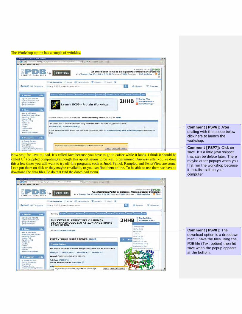
The Workshop option has a couple of wrinkles. Now wait for Java to load. It’s called Java because you have to go to coffee while it loads. I think it should be called C2 (crippled computing) although this applet seems to be well programmed. Anyway after you’ve done this a few times you will want to try off-line programs such as Jmol, Pymol, Ramplot, and SwissView are some. I can put them on disk or they maybe emailable, or you can find them online. To be able to use them we have to download the data files To do that find the download menu.
Comment [PSP6]: After dealing with the popup below click here to launch the workshop.
Comment [PSP7]: Click on save. It’s a little java snippet that can be delete later. There maybe other popups when you first run the workshop because it installs itself on your computer
Comment [PSP8]: The download option is a dropdown menu. Save the files using the PDB file (Text option) then hit save when the popup appears at the bottom.

Before we go on and discuss the viewing programs (Jmol, Pymol, Ramplot, and SwissView) in detail here’s a few pointers. The online Jmol is mainly a viewer but it has some dropdown menus at the bottom that make it a very interesting viewer. I love the way it refers to the standard text book view for proteins as cartoons. The offline Jmol is just the simple viewer in the options list. If that’s what you want go for it. Kiosk (the “other” viewer) makes a good screen display for open house. The Protein Workshop is a supped up viewer. I think it give the best pictures. There are a few bells and whistles I have checked out yet. When you first run it it installs itself on your computer. I my humble opinion Pymol is garbage. RamaPlot (Ramchandran Plot Explorer) is possibly the most interesting. It’s old and the visualization is not fancy but it seems to give stuff other programs don’t, or at least the kind of stuff relevant to this course SwissView (Swiss-PDB Viewer) Lots of options but no fancy pictures. Qutemol is interesting if you want to see the importance of lighting and shading when rendering 3D molecules. For other options see http://en.bio-soft.net/3d.html http://www.pdb.org/pdb/static.do?p=software/software_links/molecular_graphics.html