CH EM I CA L C H A R A CT ER I Z A T I O N O F UR B A N A ER O S OL S C OL L EC T E D I N

B U DA P ES T

EÖTVÖS LORÁND UNIVERSITY

Institute of Chemistry

Department of Analytical Chemistry

BERGEN UNIVERSITY COLLEGE

Department of Chemistry engineering

Institute of aqua culture-, chemistry- and bio engineering subjects

Chemistry engineering

PREFACE

The Bachelor thesis makes up 15 credit points, and it is completed during the last semester of the

bachelor degree at Bergen University College (HiB). This thesis was done at the Deparmtent of

Analytical Chemistry of the institute of Chemistry at Eötvös Loránd University, in the framework of

collaboration between Eötvös Loránd University and Bergen University College.

First of all we would like to thank our supervisor Dr. Gyula Záray for all the help we got from him

throughout the process. We would also like to give a special thanks to Viktor Gábor Mihucz and

Enikő Tatár who has been of great help to us in both the writing process and the experimental part.

Budapest, 24 June 2009

2

Linda Hanekam Nina Terese Sture

3

ABSTRACT

The goal of this thesis was to determine the concentrations of 28 elements (Li, Be, Rb, Sr, Sn, Sb, Te,

Tl, Pb, Bi, U, Ag, Cd, Pt, V, Cr, Mn, Fe, Co, Ni, Cu, Zn, Ga, As, Se, Mo, Rh, Pd) in urban aerosol collected

at three different sites of Budapest, Hungary during a 3-month sampling-campaign from April 2009

to June 2009.

The samples were taken onto quartz fibre filters with a high-volume sampler equipped with a PM 2.5

head. Once a month, one sample was collected from each of the sites with a sampling time of 96

hours. The air intake was 30 m3/h, resulting in 2880 m3 sampled air volume.

For the quantitative determination of the investigated elements a sector-field inductively coupled

plasma mass spectrometer (ICP-SF-MS) was used. Prior to the ICP-SF-MS measurements, one half of

each sample was subjected to water extraction performed in a sonication bath, while the other

halves were digested by microwave assisted acidic digestion procedure. Gold and indium were used

as internal standards.

The mass concentrations of PM2.5 were higher in Budapest than in Rome, Italy, however the

concentrations found in Budapest were lower than the concentrations found at various sites in

Spain. The mass concentration of Budapest is below the annual mean health limit value of PM 10

established by the European Union (1). The average mass concentrations found at Széna tér, Gilice

tér and behind the incinerator of Kápostásmegyer were 20.1, 21.1 and 25.2 µg/m 3, respectively,

while the mean health limit of PM10 is 40 µg/m3.

All of the elements could be determined by ICP-SF-MS in the range of 0.001-52.6 ng/m 3 for the

sample subjected to sonication assisted water extraction, and the range of 0.001-782.6 ng/m3 for

the sample subjected to microwave assisted digestion, in PM2.5 aerosol fractions collected at three

different sites in Budapest during a 3-month sampling campaign started in April 2009. The element

concentrations were the highest generally at Széna tér, a high-traffic related square of Budapest. As

expected iron, copper, antimony and tin had very high concentrations at Széna tér. However, zinc

and especially lead was found to be unexpectedly high at unexpected locations, and they should

therefore be further investigated.

4

CONTENTS

Preface.............................................................................................................................................................................................. 2

Abstract............................................................................................................................................................................................ 3

1. Introduction.............................................................................................................................................................................. 3

2. Theoretical part....................................................................................................................................................................... 3

2.1 Aerosols............................................................................................................................................................................... 3

2.1.1 Adverse Health effects..........................................................................................................................................3

2.1.2 PM investigations................................................................................................................................................... 3

2.1.3 Typical and toxic elements in aerosols.........................................................................................................3

2.2 Inductively coupled plasma mass spectrometry...............................................................................................3

2.2.1 Quadrupole mass spectrometer.......................................................................................................................3

2.2.2 Time-of-flight mass spectrometer...................................................................................................................3

2.2.3 Magnetic sector field.............................................................................................................................................3

2.3 Sampling equipment......................................................................................................................................................3

2.3.1 Samplers..................................................................................................................................................................... 3

2.3.2 Filters........................................................................................................................................................................... 3

3. Experimental.............................................................................................................................................................................3

3.1 Materials and methods................................................................................................................................................. 3

3.1.1 Reagents......................................................................................................................................................................3

3.1.2 Instrumentation...................................................................................................................................................... 3

3.2 Aerosol sampling.............................................................................................................................................................3

3.3 Sample preparation........................................................................................................................................................3

3.3.1 Pre-treatment of the filter samples................................................................................................................3

3.3.2 Microwave assisted digestion...........................................................................................................................3

5

3.3.2 Sonication assisted water extraction of the filter samples...................................................................3

4. Results and discussion..........................................................................................................................................................3

6. Conclusions................................................................................................................................................................................ 3

7. Acknowledgements................................................................................................................................................................3

Samandrag...................................................................................................................................................................................... 3

8. References.................................................................................................................................................................................. 3

Appendix A..................................................................................................................................................................................... 3

Operating conditions.............................................................................................................................................................3

Appendix B...................................................................................................................................................................................... 3

Standard solutions................................................................................................................................................................. 3

Appendix C...................................................................................................................................................................................... 3

Mass determination of the loaded quartz filters.......................................................................................................3

Appendix D..................................................................................................................................................................................... 3

Calculations............................................................................................................................................................................... 3

Appendix E...................................................................................................................................................................................... 3

Concentration values of elements determined in PM2.5 urban aerosol fractions........................................3

Appendix F...................................................................................................................................................................................... 3

Raw data..................................................................................................................................................................................... 3

6

1. INTRODUCTION

In the last years, air pollution has been receiving a lot of attention. There are plenty of sources that

causes air pollution and they are increasing as the world gets more and more industrialized. This

leads to the raising of questions like: how does this emission affect the human health and the

environment in short and long term? This may be some of the reasons that led the leaders of the

European Union to demand the member states to monitor the air pollution. Thus, the member states

have to ensure that the PM10 and PM2.5 fractions of urban aerosols are measured (1). In the previous

years plenty of research focused on the PM10 fraction, while the investigation of PM2.5 fraction has

only drawn the attention in the last couple of years due to the fact that results revealed that the

PM2.5 possibly would have more critical effects on the human health.

This thesis is written based on a three-month sampling campaign, carried out during the spring

season (April-June) of 2009 in Budapest, Hungary. The goal was to make an elemental

characterization of the collected urban aerosols corresponding to PM2.5 fractions. The ICP-SF-MS

was used to measure solutions of the samples. Two parallels were digested by microwave assisted

digestion and the other two parallels were subjected to sonication assisted water extraction.

Because of the fact that the sonication assisted water extraction is more likely to resemble

availability of the investigated elements for human beings, the results originating from this latter

method are also very important. The data acquisitions from the ICP-SF-MS measurements were

followed by the determination of the concentrations for each element.

7

2. THEORETICAL PART

Aerosols are considered as solid and liquid particles in air or in some other gas, which are smaller

than 100 µm in diameter (2). In some cases the gas is the air containing particles produced by

different formation processes like vapour condensation, combustion or mechanical disintegration of

the surface of the Earth. A part of the particles is emitted into the atmosphere from the surface

(primary particles), while other particles come into being in the air by gas-to-particle conversion

(secondary particles). Aerosol particles formed by gas-to-particle conversion either in gas or liquid

phase (e.g. in clouds) generally have sizes (diameters) below 1 µm (10 -6 m) called the fine particles.

On the other hand, surface dispersion creates particles of a diameter larger than 1 µm, termed the

coarse particles. Bio aerosols (e.g. pollens, spores) released directly by the vegetation are generally

in this latter size range. Particles due to combustion can be found in both size intervals mentioned

(3).

2.1 AEROSOLS

The aerosols found in the atmosphere today are both natural and man made. Airborne particles or

aerosols are known as “particulate matter (PM)” or simple “particles” (4). “PM10” refers to particles

smaller than 10 µm in diameter (usually 10-2.5 µm), while “PM2.5” refers to the fine particles of 2.5

µm in diameter or smaller. The major part of the aerosol of < 2 µm comprises man made

components (e.g. lead from motor exhausts, ammonium sulphate from atmospheric oxidation of

sulphur dioxide), whilst the > 2 µm material is frequently natural in origin (e.g. wind-blown soil,

marine aerosol) (5).

The aerosols in the atmosphere are often divided into two groups: the anthropogenic aerosol and

the natural aerosol. The major natural aerosols components are sea salt, soil dust (e.g. viruses,

bacteria, protozoa, algae and humic substances), natural sulphates, volcanic aerosols, and those

generated by natural forest fires (6). Anthropogenic aerosols are formed because of the human

activity, and they are in the largest amount in the big cities. These urban aerosols are often just

associated with emission from vehicles, but they are also caused by power plants, different burning

processes and other various industries. While natural aerosols are uncontrollable, urban aerosols

are controllable even though it is a challenge. This is probably why the urban aerosols attract more

8

attention within research than the natural aerosols. Large amounts of heavy elements are

discharged every day and during the past 100 years the amount of carbon dioxide in the

atmosphere has increased by about 25% on account of human activities (6). It is also a concern that

aerosols may contribute to the global warming, and have negative effects on the human health.

2.1.1 ADVERSE HEALTH EFFECTS

The concentration of many chemicals in the atmosphere has increased considerably due to

industrialization and its factory chimney emission release. Motor vehicles also produce a number of

air pollutants that pose risks to human health. Some of the traffic-generated air pollutants are

oxides of nitrogen (NOx), carbon monoxide (CO), volatile organic compounds (VOCs), and fine

particulate matter (PM2.5). Aerosols can enter the human

body via the skin, but their major route is the respiratory

system (see Figure 1). The health risk differs from one

pollutant to another, for example, nitrogen dioxide (NO2)

mainly acts as an irritant affecting the mucosa of the eyes,

nose, throat and the respiratory tract. On the other hand,

fine particles can penetrate deep into the lungs and cause

serious health problems such as irritation of the breathing

airways, difficulty in breathing, aggravated asthma,

development of chronic bronchitis and also premature

deaths in people with heart or lung disease (7).

Health effects, adverse or therapeutic, of the inhaled

particulate matter are determined by complex sets of

physiological and/or physical, chemical and biological

properties of both the respiratory system and the aerosol

(8). Urban PM has been found to contain significant

amounts of metals (9), which may mediate the health

related effects of PM exposures, as demonstrated in a

number of studies (10) (11) (12). Previous research on an

IDEAL respiratory system (mathematical model) indicated

that the highest deposition values of aerosols were observed in the extrathoracic region, regardless

of size distributions of the aerosol, or the age and gender of the human. Depositions were also

9

Figure 1: The human respiratory

system.

observed in the tracheobronichial tree and the acinar region, but in much smaller amounts (13).

Several mathematical models of the human respiratory system have been developed to be able to

calculate the deposition of the aerosols that are present regardless of size (14) (15) (16) (17) (18).

Former studies have concluded that the ultrafine particles of urban aerosols are possibly

responsible for the particle size dependence of pulmonary diseases (19), which is also indicated by

epidemiological studies (20) (21). Some other epidemiological studies as well as animal inhalation

experiments support the hypothesis that physical (e.g., particle size, shape and electrical charge)

and chemical properties (e.g., solubility or transportability) of single particles are also involved in

their potentially toxic, genotoxic and carcinogenic health effects (19). Nevertheless the fine aerosols

(PM2.5) are small enough to enter the alveoli, and it is therefore necessary to do more medical

research on the long-term effects of this exposal on the human body.

2.1.2 PM INVESTIGATIONS

In 2008, a review dealing with source apportionment of atmospheric particulate matter (PM)

between 1987 and 2007 in Europe was published (22). It pointed to four main source types for the

PM10 and PM2.5 throughout Europe: a vehicular source (traced by carbon/Fe/Ba/Zn/Cu), a crust

source (Al/Si/Ca/Fe), a sea-salt source (Na/Cl/Mg), and a mixed industrial/fuel-oil combustion

(V/Ni/SO42-) as well as a secondary aerosol (SO4

2-/NO3-/NH4

+) source (the latter two probably

representing the same source type) (22).

Until 2005, PM10 was the preferred target metric. PM10 was investigated in 46% of the publications

reported, while PM2.5 was investigated in 33%. However, in 2006 and 2007 38% of the new studies

found in the literature targeted PM2.5, while only 29% focused on PM10 (22). This shifting focus is

most likely related to the effects that fine particles have on human health.

A broad spectrum of techniques was described in the different articles (see Table 1). Ion

chromatography was most commonly used for the determination of ionic species (22% of the

studies), while major and trace elements were determined in similar proportions (9–12%) by

inductively coupled plasma atomic emission spectrometry (ICP-AES), inductively coupled plasma

mass spectrometry (ICP-SF-MS), Particle induced X-ray emission spectrometry (PIXE) and X-ray

fluorescence (XRF). Discrimination between organic (OC) and elemental (EC) carbon was only

carried out in 5% of the studies. The low percentage of OC/EC analyses, as well as the almost

10

complete absence of data on speciation of organic aerosols (OA) in these studies, implies an evident

difficulty to detect and interpret sources of organic PM, such as different vehicular sources (e.g.,

diesel vs. gasoline vehicles) (22).

In 2002 an investigation was done at four different locations in Budapest, Hungary, to determine

elemental mass size distributions and atmospheric mass concentrations of PM 10, PM2.5 and PM (23).

Fraction PM10 contributed 83, 82, 69 and 69% of the total suspended particulate in the order of the

sampling sites: KFKI campus, Lágymányos campus, Széna tér and Castel District Tunnel,

respectively, while PM2.5 made up 55, 62, 40 and 34% of PM10, respectively. By applying X-ray

emission spectrometry (XES), the mass concentration of PM0.1 fraction was found to be only

between 1.5 and 2.1% of the PM2.5 (23).

In 2006, a study analyzing the relation between air pollution (nitrogen dioxide, PM 10 and PM2.5) and

cause-specific mortality was done in a population-wide sample in Oslo, Norway (24). The goal was

to address the thresholds of different causes of death. The major sources of air pollution during the

period were car traffic, road dust, wood burning, and long-range transport by trucks (mainly for

PM2.5 and PM10) (24). The daily average exposure values from all the neighbourhoods were

calculated during the 4-year period 1992-1995 and were categorized into quartiles for each air

pollutant. The mean value for PM10 was 19 µg m-3 (range, 7-30) and for PM2.5 was 15 19 µg m-3

(range, 7-22) (24). Hazard ratios for all causes of death across quartiles of PM2.5 showed an

increasing effect for men and women in both age groups: age 51-70 and 71-90 years (24). The effect

was estimated to be largest for the youngest age group, while the effect on the women in the oldest

age group was comparatively small.

In Spain 21 different sites were monitored between 1999 and 2005 (25). The locations were: three

traffic sites, eleven urban background sites, four suburban sites with variable industrial influences

and three regional background sites. At the least polluted rural sites, most trace metal

concentrations lied within the range of 0.1-10 ng m-3, with only Zr, Mo, Ni, V, Ti, Ba, Cu, Pb, Zn (in

increasing order of abundance) exceeding 1 ng m-3. Concentrations rose with increasing

anthropogenic contamination, in the most extreme cases multiplying values to over 10 times in the

case of the rural background for Ti, Cr, Mn, Cu, Zn, As, Sn, W and Pb. Atmospheric metal particle

mixtures from the sites tend to each have their own characteristic chemical signature (25). Earth

crust related trace elements (Cs, Sr, Ti among others) measured as PM2.5 reach only 20-40% of the

levels of PM10, a percentage that in contrast increased up to 60%, 65%, 70% and 80% for As, Ni, Pb,

and Cd (25).

11

The exposure that children in the age 11-15 years had to PM2.5 during physical education at a school

was investigated in Prague, Czech Republic, in 2009 (26). The indoor concentration of PM2.5

exceeded the WHO recommended 24-hour limit of 25 µg m -3 in 50% of the days measured. The

average 24-h concentrations of PM2.5 in the school were similar to the corresponding average from

the nearest fixed site monitor, suggesting a high outdoor-to-indoor penetration rate (26). The

coarse indoor fraction concentration (PM2.5-10) was associated with the number of exercising pupils,

indicating that human activity was its main source.

The size distribution, spatial variability and temporal variability between chemical fractions of PM10

and PM2.5 were studied in Rome, Italy in 2008 (27). The soluble fractions of As, Mg, Ni, Pb, S, Sn, Tl

and V showed the same temporal pattern at the three sites suggesting spatially homogeneous

sources for the soluble species of these elements. All these, apart from Mg, were almost totally in the

fine fraction. Also the soluble fractions of Cd and Sb were almost totally in the fine fraction; however

these elements were also influenced by localized sources (27).

An experimental work regarding physical-chemical characteristics of fine aerosols was done in the

Venice Lagoon, Italy (28). Sulphate, nitrate and ammonium were largely present in the soluble

fraction of PM1.0 and PM2.5 lagoon atmospheric aerosol. The sum of these ions in the spring campaign

of 2006 varies from 51% to nearly 100% of PM2.5 fraction aerosol. By applying the PIXE and Particle

Induced Gamma-ray Emission (PIGE) analyzing techniques, ammonium was found to be

significantly correlated to non-sea-salt sulphate and nitrate, thus indicating the prevalence of

ammonium nitrate and sulphate in the samples.

There is a renewed interest in domestic wood heating as an alternative to fossil fuel and nuclear

power consumption in Sweden (29). Wood combustion is an important source of particulate matter

(inorganic ash material, condensable organic compounds, and carbon-containing particles), as well

as a source of a complex mixture of gases, some of them known as potentially carcinogenic species

(e.g. benzo[a]pyrene) (29). However, an increasing of aerosol concentration may lead to negative

effects, both on the environment and on human health. In order to characterize the urban aerosol

during the wood burning season in Northern Sweden, a field campaign was conducted in a

residential area in winter 2005/2006 (29). The focus was on the analysis of the temporal variation

and daily pattern of aerosol physical properties. The mean and standard deviation concentrations

were 12.1 ± 10.2 µg m-3 for PM10 and 9.2 ± 5.9 µg m-3 for PM1. On average, PM1 accounted for 76% of

PM10 (29). The results suggested that a combination of emissions from residential wood combustion

and traffic sources might explain the high evening concentration of PM10, PM1, particle number, and

12

light-absorbing carbon as well as large geometric mean diameters observed during weekdays and

weekends (29).

Particle number and PM2.5 concentrations were determined in the cabin of buses and trams and in

the compartment of the driver in Helsinki, Finland in 2009 (30). The average PM2.5 concentrations

were 20 to 25% lower in the compartment of the driver than in the cabin in all the monitored

vehicles independently of the vehicle age and type. It was speculated that this was connected with a

larger re-suspension of particles in the cabin space, but a proper analysis would be required before

any conclusion could be drawn. Heavy metals associated with road traffic emissions (Cu and Zn)

were elevated in the buses while emission from the wheel-trail interface probably increased the Fe

concentration, especially in the older trams (30). The results indicate that the exposure of the driver

to particles can be lowered with the existing techniques by using newer vehicles with improved air

conditioning and filtration as well as good isolation of the compartment of the driver. The low-floor

construction of newer vehicle types was not observed to lead to elevated street dust penetration

(PM2.5) inside the vehicles (30).

Table 1: Relevant particulate matter investigations in Europe between 2002 and 2008, with

emphasis on the type of particulate matter, applied techniques and investigated elements.

Year Place, Country PM Technique Elements Ref

2002 Budapest,

Hungary

10, 2.5,

0.1

XES Na, Mg, Al, Si, P, S, Cl, K, Ca, Ti, V, Cr,

Mn, Fe, Ni, Cu, Zn, Ga, Ge, As, Se, Br,

Rb, Sr, Zr, Nb, Mo, Ba, Pb,

(23)

2006 Oslo, Norway 10, 2.5 - - (24)

2007 Barcelona,

Spain

10, 2.5, 1 ICP-AES, ICP-SF-

MS,

Li, Be, P, Sc, Ti, V, Cr, Mn, Co, Ni, Cu,

Zn, Ga, Ge, As, Se, Rb, Sr, Y, Zr, Nb,

Mo, Cd, Sn, Sb,, Cs, Ba, La, Ce, Pr, Nd,

Sm, Gd, Dy, Er, Yb, Hf, Ta, W, Tl, Pb,

Bi, Th, U

(25)

2008 Prague, Czech

Republic

10, 2.5 - - (26)

2008 Rome, Italy 10, 2.5 ICP-OES, ICP-SF-

MS

Al, As, Ba, Ca, Cd, Co, Cr, Cu, Fe, Mg,

Mn, Na, Ni, Pb, S, Sb, Si, Sn, Sr, Ti, Tl,

V

(27)

13

2008 Venice Lagoon, Italy

2.5 PIXE, PIGE Na+, NH4+, K+, Mg2+, Ca2+, Cl-, NO3

-,

SO42-, C2O4

2-, F-, C2O42-, CH3COO-,

HCOO-, MSA-, CH3COCOO-

or

Na, Mg, Si, S, Cl, K, Ca, Ti, Cr, Mn, Fe,

Ni, Cu, Zn, As, Pb,

(28)

2008 Lycksele,

Sweden

10, 1 - - (29)

2009 Helsinki,

Finland

2.5 - Ca, Cu, Fe, K, Mn, S, Si, Ti, Zn (30)

2.1.3 TYPICAL AND TOXIC ELEMENTS IN AEROSOLS

In 1999, Pinheiro, T, et al. (31) investigated airborne particulate matter (PM10) found in the human

respiratory system. Both particles in the epithelial regions of trachea and bronchi were identified. In

the upper regions of the respiratory, Earth crust elements were mainly found, such as Al, Si, Ca and

Fe. Occasionally, Ti and Zn were also present. In the bronchi, the chemical composition was more

varied. Elements such as V, Cr, Mn, Fe, Cu, and Zn were detected, mainly in the association with S, K,

Ca and Si (31).

The following table (Table 2) summarizes the toxic hazard of some elements.

Table 2: The relative toxicity of cations (32). OH- stands for base (sodium hydroxide or sodium

carbonate), S2- for sulphide, SO42- for sulphate and CO3

2- for carbonate.

Name Toxic hazard Precipitant

Antimony High OH-, S2-

Bismuth Low OH-, S2-

Chromium (III) High OH-

Cobalt (II) High OH-, S2-

Copper Low OH-, S2-

Gallium High OH-

14

Iron Low OH-, S2-

Lithium Low

Manganese (II) High OH-, S2-

Molybdenum Low OH-

Nickel High OH-, S2-

Platinum (II) High OH-, S2-

Rubidium Low

Silver High Cl-, OH-, S2-

Strontium Low SO42-, CO3

2-

Vanadium High OH-, S2-

Antimony (Sb) comes probably from a corruption of an old Arabic word or from the Latin word

stibium, meaning mark (33). Antimony is a metalloid often found in contaminated soils. Auto brake

linings and brake disks are major contributors to antimony emissions along heavily travelled

highways (34). It is a toxic metalloid and is often present in inorganic forms such as more toxic

Sb(III) and less toxic Sb(V) (35).

Bismuth (Bi) comes from the German word weisse Masse, which means white mass and it is used

in low-melting alloys and in medicines that relieve indigestion (33). No industrial poisoning by

bismuth metal has ever been reported but ingestions of compounds and inhalation of dust should be

avoided (36).

Cadmium (Cd) comes from Greek Cadmus, founder of Thebes (33). It is extremely toxic and

accumulates in humans mainly in the kidneys and liver; prolonged intake, even of very small

amounts, leads to dysfunction of the kidneys (36). Normal dietary intakes are in the range 0.21-0.42

mg per week which are close to the WHO recommended maximum (0.4-0.5 mg per week) (37).

Cadmium has caused a serious disease (itai itai) in Japan from pollution. It may also pose pollution

problem associated with industrial use of zinc, e.g., galvanization (38).

Chromium (Cr) comes from the Greek word chroma that means colour and is corrosion-resistant

metal (33). The main use of the chromium metal so produced is in the production of non-ferrous

alloys, the use of pure chromium being limited because of its low ductility at ordinary temperatures

(36). It is highly toxic as CrVI and moderately toxic as CrIII (38).

15

Cobalt (Co) comes from the German word kobold, meaning goblin or evil spirit (33). It is used to

make permanent magnets and for alloying with iron. Humans need cobalt in the diet, because it is a

component of vitamin B12 (33). Extensive areas are known where low soil cobalt affects the health of

grazing animals (38).

Occupational exposure to cobalt may result in adverse health effects in different organs or tissues,

including the respiratory tract, the skin, the hemapoietic tissues, the myocardium or the thyroid

gland. In addition, teratogenic and carcinogenic effects have been observed in experimental systems

and/or in humans (39).

Copper (Cu) derived from aes cyprium (later Cuprum), since it was from Cyprus that the Romans

first obtained their copper metal (36). About one-third of the copper used is secondary copper (i.e.

scrap). The major use is as an electrical conductor but is also widely employed in coinage alloys as

well as the traditional bronze, brass, and special alloys such as Monel (Ni-Cu) (36). Wilson’s disease,

genetic recessive, results in toxic increase in copper storage (38).

Gallium (Ga) comes from Latin Gallia (33). Its main use is in semiconductor technology. For

example, GaAs can convert electricity directly into coherent light and is employed in

electroluminescent and in solid-state devices such as transistors (36). Gallium is the second metal

ion, after platinum, to be used in cancer treatment (40). Its toxicity is well documented in vitro and

in vivo in animals. In humans, the oral administration gallium is less toxic, and allows a chronic

treatment, allowing an improvement of its bioavailability in tumours, by comparison with the

parenteral use (40).

Iron (Fe) is lustrous metallic with a greyish tinge, which is most widely used of all the d-metals. It is

also the most abundant element on Earth as a whole and the second most abundant metal in the

crust on Earth (33). A healthy adult human body contains about 3 gram of iron, mostly as

haemoglobin. Close to 1 mg is lost daily (in sweat, faces, and hair), so iron must be ingested daily in

order to maintain the balance (33). It is normally only slight toxicity, but excessive intake can cause

siderosis and damage to organs through excessive iron storage (hemochromatosis) (38).

Lead (Pb) comes from Latin plumbum (41) and is an extremely toxic metal; its effect on human is

cumulative. It enters the body either as inorganic lead (Pb2+) ion or as tetraethyl lead (41). It can

lead to damage on the central nervous system and cause blood and brain disorder.

16

Lead is a worldwide pollutant of the atmosphere. It is concentrated in urban areas from the

combustion of tetraethyl lead in gasoline as well as local pollutant from mines (38).

Lithium (Li) comes from the Greek word lithos and means stone (33) and belongs to alkali metals.

It is, as all alkali metals, very reactive. The crust of the Earth is about 0.006 percent lithium by mass

and the element is also present in seawater to the extent of about 0.1 µg/g by mass (41). Breathing

in lithium dust can irritate both nose and throat. Lithium is used pharmacologically to treat manic-

depressive patients (38). However, it may be risky, since lithium has a narrow range between

therapeutic and toxic serum levels (42). It is slightly toxic (38).

Manganese (Mn) comes from Greek and Latin magnes and means magnet (33). Millions of tons of

manganese are used annually, and it is most common mineral, pyrolusite, has been used in

glassmaking since the time of the Pharaohs (36). It is moderately toxic (38).

Molybdenum (Mo) comes from the Greek word molybdos and means lead (33). It is used in the

manufacture of stainless steel and high-speed tools, which account for about 85 % of molybdenum

consumption (36). Pollution from industrial smoke may be linked with lung disease (38).

Nickel (Ni) comes from German and means Old Nick (33). Some individuals get an allergic reaction

when in skin contact with nickel, which is known as dermatitis. The reaction is marked by itching

and read skin. Nickel is very toxic to most plants. It is highly toxic to invertebrates and moderately

toxic to mammals (38).

Platinum (Pt) comes from Spanish plata and means silver (33). It is used in different fields ranging

from laboratory equipment and catalysers to dentistry. Cis-diamminedichloroplatinum(II) is used as

an anticancer drug (38). A review of airborne particulate matter, platinum group elements and

human health published in 2009 (43) concluded that platinum may pose a greater health risk than

once thought. Platinum group elements may be easily mobilised and solubilised by various

compounds present in the environment, thereby enhancing their bioavailability. They may also be

transformed into more toxic species upon uptake by organisms. A significant proportion of platinum

group elements found in airborne PM are present in the fine fraction that has been found to be

associated with increases in morbidity and mortality (43).

Rubidium (Rb) comes from the Latin word rubidus, which means deep red or flushed (33). The

main use for rubidium is for hardening platinum and palladium (36). Studies (44) indicate that

17

rubidium is only slightly toxic on an acute toxicological basis and it would pose an acute health

hazard only when ingested in large quantities.

Silver (Ag) or argentum in Latin, is rarely found native (as the metal). It is most obtained as a by-

product of the refining of copper and lead, and a considerably amount is recycled through the

photographic industry (33).

Strontium (Sr) is named after Strontian, a village in Scotland, where it was first discovered (33).

Strontium has a variety of commercial and research uses. It has been used in certain optical

materials, and it produces the red flame color of pyrotechnic devices such as fireworks and signal

flares. Strontium has also been used as oxygen eliminator in electron tubes and to produce glass for

color television tubes. Strontium ion is slightly toxic; the toxicity of its compounds is thus closely

associated with the anion of the compound concerned (45).

Tellurium (Te) comes from Latin tellus meaning earth (33). Compounds of tellurium should be

treated as potentially toxic. For instant H2Te is particularly dangerous, as it is taken up by the

kidneys, spleen, and liver, and even in minute concentrations cause headache, nausea, and irritation

of mucous membrane (36).

Thallium (Tl) comes from Greek thallos meaning green shoot (33). Both the element and its

compounds are extremely toxic; skin-contact, ingestion, and inhalation are all dangerous, and the

maximum allowable concentration of soluble thallium compounds in air is 0.1 mg m-3 (36).

Tin (Sn) is a silvery lustrous grey element, which is resistant to corrosion and is mainly used in

tinplating. It provides a non-toxic corrosion-resistant cover for sheet steel and it can be applied both

by hot dipping in molten tin, or more elegantly and controllably by electrolytic tinning. In addition

to extensive use in food packaging, tinplate is used increasingly for distributing beer and other

drinks. Tin is a non-toxic element (36).

Uranium (U) is named after the planet Uranus (33). Uranium is an emerging pollutant and it can

cause irreversible renal injury and may lead even to death which concerned the USEPA to set the

maximum permissible uranium concentration in drinking water to 30 ng/g. The environmental

impact of uranium mining and milling activities are severe as it releases hazardous and

conventional contaminants to environment (46).

Vanadium (V) comes from Vanadis (33), which is another name for the Scandinavian mythological

goddess, Freya. About 80 % of vanadium produced is used as an additive to steel. The benefit of

18

vanadium as an additive in steels is that it forms V4O5 with any carbon present, and this disperses to

produce a fine-grained steel which has increased resistance to wear and is stronger at high

temperatures (36). Vanadium is possible pollutant from industrial smoke that may cause lung

disease (38).

Zinc (Zn) occurs principally as the mineral sphalerite, ZnS, also called zincblende. Zinc is used as

anode in mercury battery. Mercury batteries are used extensively in medicine and electronic

industries, for instance in pacemakers, hearing aids, electric watches and light meters (41).

Pollution from industrial smoke may cause lung disease and the use of zinc promotes cadmium

pollution. Zinc is moderate to slightly toxic and orally causes vomiting and diarrhoea (38).

2.2 INDUCTIVELY COUPLED PLASMA MASS SPECTROMETRY

The ICP-SF-MS is based on connecting inductively coupled plasma, to produce ions, with a mass

spectrometer that separates and detects the ions, Figure 2. The most common method for

introduction of solutions into the plasma is the pneumatic nebulisation. The nebulizer converts

liquid samples into aerosols and the aerosols is subsequently passed forward into the plasma to

create ions. An ICP is a partly

ionized gas that consists of the

same amount of both negative

and positive charged particles.

It is established and maintained

by electromagnetic field with a

frequency of 27.2 MHz. The

plasma is formed in a torch

(often made of quartz) which

consists of three tubes. Mostly

pure argon gas is used as

plasma auxiliary and sample

carrier gas with flow rate of 10

L/min, 1 L/min and 0.5 L/min,

respectively. Samples to be analyzed are introduced into the central channel of the plasma where

the temperature amounts to 6000-6500 K. Due to this temperature a large proportion of the atoms

of many chemical elements are ionized by loosing its most detachable electron, to form a singly

19

Figure 2: Schematic setup of a magnetic sector field inductively

coupled plasma mass spectrometer (48).

charged ion. The ions are extracted through a sampler cone and further through a skimmer cone

into a mass spectrometer, which operates in a high vacuum. Approximately 75 elements and 300

isotopes can be resolved at the same time (47). The MS consists of three modules: an ion source, a

mass analyzer and a detector. Here the ICP is the ion source. The mass analyzer is applying an

electromagnetic field to sort the ions by masses, while the detector measure the value of an

indicator quantity and thus provides data for calculating the abundances of each ion present.

Inductively coupled plasma mass spectrometers generally incorporate one of two basic detection

schemes: Faraday cup detectors, or electron multiplier detectors (48). Mass spectrometers produce

various types of data; the most common data representation is probably the mass spectrum. Other

types of mass spectrometry data can be mass chromatogram, types of chromatograms that include

selected ion monitoring (SIM), selected reaction monitoring chromatogram (SRM) and total ion

current (TIC). There is also a possibility to use three dimensional contour maps (48).

According to A.L. Gray (49) only mass spectrometry offers the combination of simple spectra,

adequate resolution and low detection limits that were desirable for trace determination in complex

matrices.

2.2.1 QUADRUPOLE MASS SPECTROMETER

Principle:

The quadrupole consists of four parallel metal

rods to which are applied both a constant voltage

and a radiofrequency oscillating voltage, Figure 3.

Over the radiofrequency voltage a direct current

voltage is superimposed. The electric field

deflects ions in complex trajectories as the ions

move towards the detector, other ions collide

with the rods and are lost before they reach the

detector, allowing only ions with one particular

mass-to-charge ratio to reach the detector. By

rapidly varying voltages one can select ions of different masses to reach the detector (47). In the

ICP-QP-MS device a DRC (dynamic reaction cell) is often placed before the quadrupole chamber to

20

Figure 3: Quadrupole mass spectrometer. Ideally,

the rod should have a hyperbolic cross section on

the surfaces that face one another (47).

reduce or eliminate spectral interferences. The DRC is filled with a low pressure reaction gas (or a

mixture of two different gases) which reacts with the molecule ions and therefore removes some of

the interference before the ions reach the quadrupole chamber (50).

2.2.2 TIME-OF-FLIGHT MASS SPECTROMETER

Principle:

In ICP-TOF-MS the ions are detected according to their m/z ratio by means of their flight times.

After the ions are being sampled from the plasma, all of them (ideally) accelerate to the same kinetic

energy. They however do not have the same flight time because their flight time is determined by

the equations:

where Ekin is the kinetic energy of the ion, m is the

ions mass, v is its velocity, z is its charge, q is the

electronic charge, U is the electrostatic potential

and L is the length of the electrostatic field-free

drift region through which the ion travels through

the detector (48). As one can see the lighter ions

will achieve higher velocity than the heavier ions

within the flight tube. This will give the ions different flight times as displayed in Figure 4. As the

ions reaches the detector a mass spectrum will be

produced at once.

2.2.3 MAGNETIC SECTOR FIELD

21

Figure 4: Time-of-flight mass spectrometer. Positive ions

are accelerated out of the source by voltage +v periodically

applied to the back plate. Light ions travel faster and reach

the detector sooner than heavier ions (47).

Principle:

The analyzer consists of a curved flight tube, which is located between the poles of either a

permanent magnet or, in practice, an electromagnet with variable field strength. The ions

(generated in the ICP) are accelerated after passing the interface region by a high extraction

potential. Positively charged ions from the plasma are focused through a sequence of ion lenses

before travelling through a narrow slit of adjustable width (source slit). Furthermore the ions are

injected perpendicular to the magnetic field and traverse the field in different circular trajectories

according to their mass/charge ratio. A second slit (collector slit) positioned at the exit of the

magnet at the focus point results in the selection of a specific mass, Figure 2, (48).

Double-focusing:

The term “double-focusing” is applied to mass spectrometers in which the directional and energy

aberrations of a population of ions are simultaneously minimized, thereby improving the resolution

capabilities of the instrument. Double focusing is achieved by the use of the combination of an

energy-focusing electrostatic field (ESA), located either prior to or after the magnetic field, and the

magnet (48).

In the Nier–Johnson geometry device a 90°

electric analyzer is placed before a 60°

magnetic sector, in which the electrostatic

analyzer field is used to compensate for

the energy dispersion. In use of the

reverse geometry the magnetic field is

placed before the electrostatic analyzer, as

indicated in Figure 5. The geometry in it

self keeps the noise down because the bend prevents the photons from going directly to the

detector, and high transmission is therefore permitted. But the reverse design also appears to

improve the abundance sensitivity and to reduce noise even more because the high ion currents

from the magnetic source are first reduced by mass analysis, and only ions of the selected mass are

subjected to the subsequent energy analysis. To enhance abundance sensitivity in this device, a wide

aperture retarding potential (WARP) filter is applied (48).

22

Figure 5: Operation principle of a double-focusing mass

spectrometer (48).

Interferences:

Operating a mass spectrometer at a high resolution is one of the most utilized ways to overcome the

problem of interferences. High mass resolution allows separation of the peak of the isotope of

interest and the interfering species (48). One of the ways to achieve higher resolution is to use a slit

system, which is found in double-focusing sector field mass spectrometers. A

slit system is equipped with slits of different dimensions, as displayed in

Figure 6, whereas each slit has the shape of a trapezoidal. The slit with the

largest dimensions attain low resolution (R=300). By decreasing the slit

width, the resolution will be increased. The slit with the smallest dimensions

will be able to attain a high resolution (R=10 000). A mass resolution of up to

10 000 and more, which is defined here as “high” resolution, is usually

achieved with double-focusing instruments (51).

Isobaric interferences are caused by overlapping isotopes of different elements of essentially the

same mass. Most elements in the periodic table have at least one, two or even three isotopes free

from isobaric overlap (49). For natural elements the isobaric interferences can be found from mass

36 to mass 204 and for non-natural isotopes they can be found in range above m/z 230, derived

from nuclear processes (48).

Molecular ion interferences are formed by the matrix elements, the atom of the solvent and/or the

atoms of the plasma gas (48). They may also arise from the reagents used for sample pre-treatment.

Another important source of molecular ions is formation of cluster ions from the dominant species

in the plasma, which preferentially occurs in cool plasma boundaries (possibly at the walls of the

skimmer) or in the sampling and expansion areas of the interface (51).

The following table (Table 3) is pointing out the advantages and disadvantages of the mass

spectrometers that are mentioned earlier.

Table 3: Advantages and disadvantages of the differents mass spectrometers.

Mass

spectrometer

Advantages Disadvantages

23

Figure 6: The slit width defines the ion

beam entering the magnetic field.

Narrow slits are used for high

resolution.

Magnetic

sector field

High mass resolution (up to 12000)

(48).

High sensitivity (48).

Low noise (48).

Good isotope ratio precision (48).

Flat-top peaks (trapezoidal shape)

(48).

High linear dynamic range over nine

orders of magnitude (48).

High cost (48).

Duty cycles limited by hysteresis

of magnetic field (48).

Loss of sensitivity at higher

mass resolution (48).

Loss of trapezoid peak shape at

high mass resolution (48).

No solution for interferences

with mass resolutions of more

than 12000 (48).

Time of flight Simple (47).

High acquisition rate (102 to 104

spectra/s) (47).

Capability for measuring very high

masses (m/z ≈106) (47).

TOF-MS seems to be an attractive

alternative to scanning-based

systems for hyphenated speciation

analysis (48).

Requires a low operating

pressure (10-12 bar) (47).

Poorer detection limits than

those obtained by quadrupole

and magnetic sector

instruments (48).

The sensitivity of ICP-TOF-MS is

much as an order of magnitude

poorer than comparable

quadrupole systems (48).

Quadrupole Good multi -purpose instrument

(47).

Reasonable price (48).

High operating pressure (10-9 bar)

(47).

Abundance sensitivity can be 106 or

better (48).

Peak tailing (48).

Ions are lost in the region of the

mass filter near the entrance,

and to a lesser extent in the

region near the exit (48).

Eliminations of spectral

interferences need DRC.

2.3 SAMPLING EQUIPMENT

24

A particulate sampling train consists of the following components: air inlet, particulate separator or

collecting device, air flow meter, flow rate control valve, and air mover or peristaltic pump. Of these,

the most important component is the particulate separator. The separator may consist of a single

element (such as a filter or impinge), or there may be two or more elements in a series (such as a

two-stage cyclone or multi-stage impactor) so as to characterize the particulates into different size

ranges (4).

2.3.1 SAMPLERS

There are two main types of samplers suitable for sampling aerosols in the ambient atmosphere –

high-volume samplers and low-volume continuously recording samplers. For applications where

aerosol concentrations are expected to be low, or when the concentrations are specific compounds

within the aerosol are low (such as dioxins, etc.), a sampler with a high flow rate is preferred. Low-

volume continuously recording samplers is used for remote automatic sampling networks, or the

study of short-term trends in the fraction of ambient aerosol to identify periods of high potential

risk (52).

2.3.2 FILTERS

Sampling on filters is the most practical method currently available to characterize the particle sizes

and chemical composition of airborne particulates (4). Airborne particles are collected from the air

surrounding the filter by a pump, while all gases pass through the filter.

Filter types for aerosol sampling are in general divided in two main categories – fibrous filters and

membrane filters. Fibrous fibres consist of layers of fibres made generally of glass, quartz or

cellulose. While membrane filters contain small pores of controlled size, and they are usually

composed of thin films of polymeric material (3).

The characteristics of different types of fibrous and membrane filters widely used for sampling

aerosol particles for subsequent chemical analysis are summarized in Table 4 .

Table 4: Properties of filters used for particulate sampling with a face velocity of 10 cm s -1. Note

that the efficiencies refer to particles with diameters above 0.03 µm (3).

Filter Composition Density (mg cm-2) Surface reactivity Efficiency (%)

25

Teflon Polytetrafluoro-ethene 0.5 Neutral 99

Whatman 41 Cellulose fiber 8.7 Neutral 58

Whatman GF/C Glass fiber 5.2 Basic (pH 9) 99

Gelman Quartz Quartz fiber 6.5 pH 7 98

Nuclepore Polycarbonate 0.8 Neutral 93

Milipore Cellulose acetate/nitrate 5.0 Neutral 99

Teflon, quartz and Nuclepore filters give the best substrates for chemical studies, because they don’t

react with atmospheric trace gases resulting in a sampling artefact (3).

26

3. EXPERIMENTAL

The sampling sites were located in three different places of Budapest, the capital of Hungary, which

includes a population of 1.7 million. The three sampling sites were Széna tér with mainly traffic

pollution, Gilice tér an urban background site and Káposztásmegyer which is located just behind a

waste incinerator.

3.1 MATERIALS AND METHODS

3.1.1 REAGENTS

Throughout the experiments, ion-exchanged water was used. Commercially available 1000 mg/L standard solutions (Pt, Sb, In, Au) were diluted and used as internal standards, while the multi element standard solution was mixed from standard solutions from Merck, Darmstadt, Germany (). For the microwave assisted digestion and acidification of the samples, hydrochloric and nitric acids of Suprapure grade (Merck, Darmstadt, Germany) were applied. All samples and standards were stored in polyethylene bottles. Standard solutions were prepared daily.

3.1.2 INSTRUMENTATION

For aerosol sampling, a Greenlab DHA-80 type high-volume PM2.5 sampler with 500 L/min air intake

was used, property of the National Meteorological Service. Ion-exchanged water (16.8 MΩ cm) was

used was produced by a PUR1TE (Purite, Thame, Oxfordshire, UK) system. Microwave assisted

digestion was achieved in an Anton-Paar GmbH MultiwaweTM equipment equipped with 6 quartz

vessels. For water extraction of the filter samples an Elma®, S40 Elmasonic, sonication bath was

applied. For the ICP-SF-MS measurements, an inductively coupled plasma sector field mass

spectrometer ELEMENT2 (Thermo Finnigan, Bremen, Germany) were used. The operating

conditions are listed in the Appendix A.

3.2 AEROSOL SAMPLING

The collection of aerosol samples was achieved in collaboration with the National Meteorological

Service, who has a network consisting of 11 completely automated air quality measuring stations in

the charge of the Environmental, Nature Protection and Hydrological Inspectorate of the Central

Danube Valley. The compounds that they usually monitor are: nitrogen dioxide, sulphur dioxide,

27

ozone, BTEX and PM10 fractions. PM2.5 collection has still not been implemented in all of the stations

on a regular basis. The sampling campaign lasted 3 months from April 2009 to June 2009 and

consisted of almost one-week long sampling periods each month at the following three sites; Széna

tér, the vicinity of an incinerator situated in Káposztásmegyer and Gilice tér. The first two sites are

located in Buda; meanwhile Gilice tér is in Pest (see Figure 7). The sampling sites were chosen in

order to collect samples from a high-traffic area (Széna tér) and from a waste incinerator zone. The

site corresponding to the Gilice tér resembled the urban background area.

Figure 7: The location of the three sampling sites (red dots) displayed in a map of Budapest,

Hungary.

The duration of the sampling was 96 hours (4 days), which resulted in a sampled air volume of 2880

m3 for the sampling period. The weather conditions during the sampling period were similar. Even

though the spring of 2009 has been quite warm, and April has been the warmest April since 1901,

the temperatures during the sampling has been quite stabile. The average temperatures during the

week of sampling in April, May and June were 15-16, 13-16.5 14-16°C, respectively. Mostly there

has been no precipitation during the sampling time, but in the last couple of days of the sampling in

June there was some precipitation.

28

3.3 SAMPLE PREPARATION

3.3.1 PRE-TREATMENT OF THE FILTER SAMPLES

For each series of measurements, four quartz filters, one for each sampling site and one blank

sample, were heated in an oven at 550°C for eight hours in order to eliminate organic contamination.

Whatman QM-A filters with a diameter of 150 mm were used. The filters were weighed, attached to

grinds, put in Petri dishes and stored in an exsiccator. Filters were handled and cut with a ceramic

scalpel and silicon tweezers, respectively. To determine the weight of the aerosol sample alone, the

filters were weighed on an analytical scale both before and after the aerosol sampling ( Appendix C).

The cut filters, later subjected to microwave assisted digestion or sonication, were also weighed.

3.3.2 MICROWAVE ASSISTED DIGESTION

For the microwave assisted digestion, ¼ of the original filter was cut out. Furthermore, the ¼ pieces

were split into two 1/8 pieces and weighed. These pieces were placed into microwave assisted

digestion quartz vessels (priory washed with nitric acid and rinsed with water). Then, aqua regia

(2.5 ml nitric acid and 7.5 ml hydrochloric acid) was added to the samples. The quartz vessels were

placed in a carousel, and put into a microwave assisted oven where a microwave assisted digestion

program was applied (Appendix A).

After the microwave assisted digestion, each liquid sample from the quartz containers was

transferred into PP (polypropylene) Falcon test tubes. The filter pieces were still intact; therefore it

was necessary to wash them carefully in order to be able to transfer the whole sample into the test

tubes. Furthermore the test tubes, containing the samples, were filled up with ion-exchanged water

up to 50 ml. Because of the fact that the test tubes now also contained colloidal particles, the

samples also had to be filtered. To strain off the particles, a MILIPORE Millex syringe filter unit (0.22

µm diameter) was utilized. After the filtration, 15 ml of the samples were transferred into 15-ml PP

Falcon test tubes previously soaked with 20% nitric acid solutions and rinsed three times with ion-

exchanged water.

3.3.2 SONICATION ASSISTED WATER EXTRACTION OF THE FILTER SAMPLES

From the loaded filters, another ¼ pieces were cut off and weighed. Furthermore, it was cut into

smaller pieces, which were put into 50-ml PP Falcon test tubes and the test tubes were filled with

29

ion-exchanged water. The tubes were put into a sonication bath for 150 minutes. After the

sonication, the solutions were filtered by applying a MILIPORE Millex syringe filter unit (0.22 µm

diameter). From the filtrate, 10 ml was extracted and mixed with 560 µl cc. nitric acid and 10 µl In,

Au (50 µg/cm3) used as internal standards for the ICP-SF-MS measurements.

30

4. RESULTS AND DISCUSSION

The concentrations for all of the elements for each site in all of the months have been compiled in

tables in Appendix E. However, some of the elements monitored could not be detected because their

concentration fell either under the detection limit (LOD) or the ICP-SF-MS could not detect the

elements at all (see Table 5 and Table 6). The concentration of the elements subjected to sonication

assisted water extraction ranged between 0.001 ng/m3 and 52.6 ng/m3, while the concentration of

the elements subjected to microwave assisted digestion ranged between 0.001 ng/m3 and 782.6

ng/m3.

Table 5: Overview of the elements, subjected to the sonication assisted water extraction, whose

concentration fell under the limit of detection (LOD) or was not detected by the ICP-SF-MS at all.

Month/ Location Not detectable < LOD

April 2009

Széna tér

Gilice tér Pt, Rh

Incinerator

(Káposztásmegyer)

Pt, Rh

May 2009

Széna tér Be, U

Gilice tér Be, U, Pt, Rh

Incinerator

(Káposztásmegyer)

Be, U Pd

June 2009

Széna tér Be, U, Ag Pt

Gilice tér Be, U, Ag Pt

Incinerator

(Káposztásmegyer)

Be, U, Ag Pt

31

Table 6: Overview of the elements, subjected to the microwave assisted digestion, whose

concentration fell under the limit of detection (LOD) or was not detected by the ICP-SF-MS at all.

Month/ Sampling site Not detectable < LOD

April 2009

Széna tér

Gilice tér Be, Pt, Co, As, Se, Pd

Káposztásmegyer Pt, As, Se

May 2009

Széna tér As, Se Pt

Gilice tér As, Se, Be, Pt, Co, Rh

Káposztásmegyer As, Se, Co, Pt, Rh Pd

June 2009

Széna tér Li, Be, U, Pt, As, Se, Rh,

Ni

Gilice tér Li, Be, U, Pt, As, Se, Rh

Káposztásmegyer Li, Be, U, Pt, As, Se, Rh

As displayed in Figure 8 and Figure 9, the concentration of the elements (subjected to sonication

assisted water extraction) has generally decreased from April 2009 to May 2009. If data of Figure 8

and Figure 10 are compared, one can also see that the concentrations of the elements have also

generally decreased from April 2009 to June 2009, with exception of arsenic (As) and zinc (Zn).

However, the concentration of the elements has increased for most of the elements from May 2009

to June 2009, which leads to the belief that some of the reason why the concentration has decreased

to this extent from April to May and from April 2009 to June 2009, may be that the mass

concentration (Appendix E, Table 24) is higher in April than in the other two months.

32

* The concentration of iron (Fe) has been decreased 10 times to make the concentration of the other determined elements more visible.

Figure 8: Concentration of the elements subjected to sonication assisted water extraction, in PM2.5

aerosol fractions collected in April 2009 at the three selected sites of Budapest.

* The concentration of iron (Fe) has been decreased 10 times to make the concentration of the other determined elements more visible.

Figure 9: Concentration of the elements subjected to sonication assisted water extraction, in PM2.5

aerosol fractions collected in May 2009 at the three selected sites of Budapest.

33

* The concentration of iron (Fe) has been decreased 10 times to make the concentration of the other determined elements more visible.

Figure 10: Concentration of the elements subjected to sonication assisted water extraction, in

PM2.5 aerosol fractions collected in June 2009 at the three selected sites of Budapest.

As expected the highest concentration of both iron (Fe), copper (Cu), antimony (Sb) and tin (Sn) was

found in Széna tér for each sampling months. This is in accordance with former European

publications (see 2.1.2 PM investigations or (22)), in which was stated that traffic and vehicle

exhaust was one of the major sources for Fe and Cu emission. Both auto brake linings and brake

disks are sources of the Sb emissions (22), which explain the high concentration found at both Széna

tér and Káposztásmegyer. Although it was expected to find the highest concentration of zinc at

Széna tér, since the main source of zinc emission is the same as the main source for iron and copper,

this was not the case. Zinc was found to have its highest emission at Gilice tér (the urban

background) in both May 2009 and June 2009. The concentration of lead (Pb) was found to be a

little bit high, especially at Gilice tér. Further research is therefore necessary, both to monitor the

concentration and to look for possible sources.

In Figure 11 the mass concentration is compared with the PM10 annual mean health limit value, set

by EU, due to the fact that there is no current existing annual health limit value for PM2.5.

34

Figure 11: PM2.5 mass concentration compared with the annual mean limit value for PM 10, set by

the European Union.

As Figure 11 shows, the mass concentrations from April 2009 to June 2009 are under the mean

health limit value. The average mass concentration found in Széna tér, Gilice tér and

Káposztásmegyer were 20.1 µg/m3, 21.1 µg/m3 and 25.2 µg/m3, respectively, while the mean health

limit of PM10 is 40 µg/m3. If the average mass concentrations are compared to previous works, it is

possible to see that the mass concentration in Budapest is higher than the mass concentration in

Rome, Italy (27). However it is lower than the mass concentration in various sites in Spain (25).

The concentration values of elements determined in PM2.5 fractions by ICP-SF-MS after microwave

assisted digestion are presented in Table 7, Table 8 and Table 9.

The total concentration is considered to be obtained by microwave assisted digestion. Because of

the fact that the concentrations obtained by the sonication assisted water extraction are the

concentrations that are most available for human beings. Due to this fact it is possible to get an

impression of what elements is expected to be absorbed by the respiratory system.

Table 7: The element concentrations of PM 2.5 aerosol samples collected, at three different sites, in

April 2009 and subjected to microwave assisted digestion. Results originating from two parallel

measurements; c = concentration; SD = standard deviation.

Elemen Széna tér Gilice tér Incinerator

35

t

(Káposztásmegyer)

c ± SD (ng/m3) c ± SD (ng/m3) c ± SD (ng/m3)

Li 1.7866 ± 0.1365 0.2205 ± 0.0075 1.7451 ± 0.1263

Be 0.2072 ± 0.0199 - 0.1478 ± 0.0141

Rb 0.6949 ± 0.2219 0.8801 ± 0.0229 0.8773 ± 0.3689

Sr 0.8204 ± 0.2306 0.9240 ± 0.0080 1.2164 ± 0.4886

Sn 384.9768 ± 115.0546 1.6986 ± 0.0196 358.7118 ± 142.5627

Sb 540.7024 ± 142.9713 5.2661 ± 0.0828 782.5842 ± 269.7238

Te 0.0392 ± 0.0046 0.0419 ± 0.0014 0.0459 ± 0.0078

Tl 0.0302 ± 0.0053 0.0529 ± 0.0013 0.0162 ± 0.0035

Pb 23.9200 ± 5.6085 31.8144 ± 0.4494 21.5919 ± 6.0315

Bi 0.1912 ± 0.0516 0.0837 ± 0.0015 0.1424 ± 0.0488

U 0.0296 ± 0.0078 0.0166 ± 0.0005 0.0236 ± 0.0085

Ag 8.7008 ± 2.6688 3.1898 ± 0.0939 4.3333 ±1.6415

Cd 1.3010 ± 0.3286 1.6062 ± 0.0304 1.4524 ± 0.5817

Pt 0.0073 ± 0.0021 - -

V 1.3277 ± 0.2209 1.3122 ± 0.0462 1.2721 ± 0.3516

Cr 2.5402 ± 0.5477 1.3449 ± 0.0319 1.3941 ± 0.3322

Mn 16.6033 ± 2.2808 7.8410 ± 0.1716 11.7301 ± 2.6897

Fe 508.0692 ± 100.5101 323.9420 ± 7.7783 363.5036 ± 63.5791

Co 0.1377 ± 0.0206 - 0.1282 ± 0.0243

Ni 6.9324 ± 1.1201 1.0323 ± 0.0207 3.5492 ± 0.6285

Cu 25.5373 ± 2.7663 17.8531 ± 0.4478 15.4213 ± 3.1849

Zn 129.1941 ± 24.6756 9.0968 ± 0.3057 110.1591 ± 18.9971

Ga 0.1807 ± 0.0338 0.1653 ± 0.0090 0.1592 ± 0.0394

As 15.3139 ± 1.7464 - -

Se 155.0285 ± 16.8307 - -

Mo 1.2731 ± 0.2491 0.3938 ± 0.0218 0.6413 ± 0.1292

Rh 0.0141 ± 0.0030 - 0.0007 ± 0.0001

Pd 0.0959 ± 0.0144 - 0.0881 ± 0.0109

36

Table 8: The element concentrations of PM 2.5 aerosol samples collected, at three different sites, in

May 2009 and subjected to microwave assisted digestion. Results originating from two parallel

measurements; c = concentration; SD = standard deviation.

Element Széna tér Gilice tér Incinerator

(Káposztásmegyer)

c ± SD (ng/m3) c ± SD (ng/m3) c ± SD (ng/m3)

Li 0.2069 ± 0.0069 0.0901 ± 0.0045 0.3325 ± 0.0111

Be 0.0134 ± 0.0005 - 0.0117 ± 0.0003

Rb 0.2518 ± 0.0057 0.3364 ± 0.0032 0.8924 ± 0.0113

Sr 0.4456 ± 0.0054 0.3585 ± 0.0022 1.1241 ± 0.0198

Sn 0.9990 ± 0.0113 0.6724 ± 0.0047 0.7477 ± 0.0069

Sb 1.3300 ± 0.0247 0.9259 ± 0.0115 1.2004 ± 0.0153

Te 0.0133 ± 0.0005 0.0151 ± 0.0005 0.0137 ± 0.0005

Tl 0.0132 ± 0.0004 0.0153 ± 0.0004 0.0168 ± 0.0005

Pb 3.8838 ± 0.0573 5.6765 ± 0.1014 6.8961 ± 0.1147

Bi 0.0817 ± 0.0024 0.1098 ± 0.0031 0.0626 ± 0.0011

U 0.0069 ± 0.0002 0.0081 ± 0.0002 0.0206 ± 0.0003

Ag 1.7218 ± 0.0448 5.0069 ± 0.1984 3.5822 ± 0.1196

Cd 0.2418 ± 0.0055 0.2723 ± 0.0082 0.2590 ± 0.0054

Pt 0.0081 ± 0.0002 - -

V 0.4396 ± 0.0213 0.5325 ± 0.0191 1.1979 ± 0.0519

Cr 1.1766 ± 0.0374 0.5954 ± 0.0146 1.3016 ± 0.0342

Mn 5.6525 ± 0.1415 3.5424 ± 0.0918 9.7727 ± 0.2368

Fe 257.7546 ± 4.3674 125.9903 ± 1.5944 414.1383 ± 5.7418

Co 1.8974 ± 0.0528 - -

Ni 0.5458 ± 0.0159 0.7996 ± 0.0210 0.9720 ± 0.0290

Cu 8.1615 ± 0.1641 5.3185 ± 0.0685 8.2791 ± 0.1808

Zn 2.7683 ± 0.0537 3.0145 ± 0.1137 1.3633 ± 0.0399

Ga 0.0535 ± 0.0030 0.0618 ± 0.0042 0.1669 ± 0.0094

37

As - - -

Se - - -

Mo 0.3567 ± 0.0214 0.2948 ± 0.0159 0.2501 ± 0.0127

Rh 0.0051 ± 0.0002 - -

Pd 0.0642 ± 0.0030 0.0620 ± 0.0031 0.3151 ± 0.0117

Table 9: The element concentrations of PM 2.5 aerosol samples collected, at three different sites, in

June 2009 and subjected to microwave assisted digestion. Results originating from two parallel

measurements; c = concentration; SD = standard deviation.

Element Széna tér Gilice tér Incinerator

(Káposztásmegyer)

c ± SD (ng/m3) c ± SD (ng/m3) c ± SD (ng/m3)

Li - - -

Be - - -

Rb 0.172 ± 0.004 0.146 ± 0.003 0.167 ± 0.003

Sr 0.297 ± 0.007 0.122 ± 0.002 0.124 ± 0.001

Sn 1.047 ± 0.009 0.484 ± 0.006 0.484 ± 0.007

Sb 0.989 ± 0.012 0.629 ± 0.009 0.676 ± 0.006

Te 0.003 ± 0.000 0.006 ± 0.000 0.005 ± 0.000

Tl 0.004 ± 0.000 0.013 ± 0.000 0.009 ± 0.000

Pb 4.311 ± 0.066 4.245 ± 0.069 4.360 ± 0.054

Bi 0.077 ± 0.002 0.027 ± 0.001 0.031 ± 0.001

U - - -

Ag 3.412 ± 0.109 1.122 ± 0.030 1.321 ± 0.023

Cd 0.201 ± 0.006 0.211 ± 0.005 0.206 ± 0.005

Pt - - -

V 0.390 ± 0.014 0.359 ± 0.012 0.412 ± 0.012

Cr 0.782 ± 0.030 0.350 ± 0.011 0.441 ± 0.011

Mn 3.585 ± 0.081 2.272 ± 0.050 2.456 ± 0.068

Fe 199.358 ± 3.223 79.436 ± 0.969 97.576 ± 0.868

38

Co 0.033 ± 0.001 0.046 ± 0.001 0.042 ± 0.002

Ni - 0.050 ± 0.001 0.252 ± 0.006

Cu 6.999 ± 0.162 2.759 ± 0.070 3.939 ± 0.071

Zn 15.330 ± 0.177 14.043 ± 0.152 14.813 ± 0.295

Ga 0.029 ± 0.002 0.017 ± 0.001 0.018 ± 0.001

As - - -

Se - - -

Mo 0.300 ± 0.023 0.133 ± 0.009 0.179 ± 0.009

Rh - - -

Pd 0.021 ± 0.001 0.003 ± 0.000 0.013 ± 0.001

39

6. CONCLUSIONS

This work is a pilot study since the PM2.5 aerosol fractions are not as regularly investigated as the

PM10 fractions. Moreover, health limit values have not been set by the decision makers of the EU for

the investigated elements. However, from the present work, the following conclusions can be

drawn:

1. All of the elements could be determined by ICP-SF-MS in the range of 0.001-52.6 ng/m3 for

the sample subjected to sonication assisted water extraction, and the range of 0.001-782.6

ng/m3 for the sample subjected to microwave assisted digestion, in PM2.5 aerosol fractions

collected at three different sites in Budapest during a 3-month sampling campaign started in

April 2009.

2. The element concentrations were the highest generally at the Széna tér, where the traffic

density amounts to about 85 000 vehicles/day.

3. The mass concentration of the PM2.5 fractions did not exceed the 40 µg/m3 annual health

limit value. The mass concentrations found in Budapest is higher than the mass

concentrations found in Rome, Italy, however it is lower than the mass concentrations found

at various sites in Spain.

4. As expected iron, copper, antimony and tin had very high concentrations at the high traffic

site, Széna tér. However, zinc and especially lead was found to be unexpectedly high at

unexpected locations, and they should therefore be further investigated.

The results of the present work are important as they could be useful for the EU decision makers in

order to establish health limit values for the elements found in PM2.5 urban aerosol fractions.

Further prospects connected to this work include accuracy test performed with standard reference

materials; investigation of seasonal variation of element concentration in PM2.5 fractions as well as

speciation studies for antimony, an element whose emission has been increased drastically lately, in

order to see to which extent are present in their toxic chemical forms in the investigated fractions.

40

7. ACKNOWLEDGEMENTS

The help and support of the following legal entities and persons is acknowledged:

Norwegian - Hungarian Foundation

National Meteorological Service

Ove Jan Kvammen, Associate professor, HiB, Norway

Kristin Kvamme, Assistant professor, HiB, Norway

Gyula Záray, DSc, Head of Department of Analytical Chemistry, Institute of Chemistry, ELTE, Hungary

Imre Salma, DSc, Department of Analytical Chemistry, Institute of Chemistry, ELTE, Hungary

Enikő Tatár, PhD, Associate professor, Department of Analytical Chemistry, Institute of Chemistry, ELTE, Hungary

Viktor Gábor Mihucz, PhD, lecturer, Department of Analytical Chemistry, Institute of Chemistry, ELTE, Hungary

Mihály Óvári, PhD, lecturer, Department of Analytical Chemistry, Institute of Chemistry, ELTE, Hungary

Szilvia Keresztes, PhD student, Department of Analytical Chemistry, Institute of Chemistry, ELTE, Hungary

41

SAMANDRAG

Føremålet med hovudoppgåva var å bestemme konsentrasjonen til 28 element ved tre forskjellige

stadar i Budapest, Ungarn, i løpet av ein 3 månadar lang måle kampangje frå April til Juni 2009.

Prøvane vart tatt på quartz fiber filter med ein høg-volum prøvetakar, som var utstyrt med eit PM 25

hovud. Ein gong i månaden samla ein inn ein prøve frå kvar av målestadane. Prøvetida var på 96

timar, der ein fekk sampla inn 2880 m3 luft volum (30 m3/t). For å måle konsentrasjonane nytta ein

ICP-SF-MS. På førhånd vart halvparten av kvar prøve behandla med vass ekstraksjon medan den

andre halvparten vart behandla med mikrobølgje ekstrahering. Ein såg på følgjande element: Li, Be,

Rb, Sr, Sn, Sb, Te, Tl, Pb, Bi, U, Ag, Cd, Pt, V, Cr, Mn, Fe, Co, Ni, Cu, Zn, Ga, As, Se, Mo, Rh, Pd. Au og In

var intern standardar.

Ein fann at masse konsentrasjonane var høgare i Budapest enn i Roma i Italia, men dei var derimot

lågare enn konsentrasjonane funne ved forskjellege stader i Spania. Likvel var masse

konsentasjonen i Budapest lågare enn den gjennomsnittlege årlege helse grensa til PM10, som er sett

av EU. Den gjennomsnittlege masse konsentrasjonen ved Széna tér, Gilice tér og Káposztásmegyer

var 20.1, 21.1 og 25.2 µg/m3, respektivt, medan gjennomsnittleg årleg helse verdi for PM10 er 40

µg/m3.

Etter å ha samla PM2.5 fraksjonar i tre månader (som vart starta opp i april 2009) frå tre ulike stader

i Budapest, kom ein fram til at ein ved hjelp av ICP-SF-MS kunne bestemme ein konsentrasjonen på

alle 28 elementa, i konsentrasjonsområdet 0.001-52.6 ng/m3 for dei prøvane som var behandla med

vass ekstraksjon og konsentrasjonsområdet 0.001-782.6 for dei prøvane som var behandla med

mikrobølgje ekstrahering. Generelt var konsentrasjonen til elementa ein fann høgast ved Széna tér,

som var rekna som området der trafikkmengda var størst. Dei høgaste konentrasjonane av elementa

jern, kopar, antimon og tinn som stort sett kjem frå trafikk relaterte kjelder fann ein difor på Széna

tér. Sjølv om ein og hadde venta å finne dei høgaste konsentrasjonane av sink på same staden, av

same grunn, var dette ikkje tilfellet. Både bly og sink hadde uventa høg konsentrasjon på andre

områder enn ein venta, så vidare forsking er naudsynt.

42

8. REFERENCES

1. Council Directive 1999/30/EC. Muller, W. 22 April 1999, Official Journal of the European

Communities, Vol. L 163, p. 41.

2. Manahan, S E. Environmental chemistry. sixth edition. s.l. : Lewis publishers, 1994. 1-56670-088-

4.

3. Mészáros, E. Fundamentals of athmospheric aerosol chemistry. Budapest : Akadémiai kiadó, 1999.

963-05-7624-4.

4. Cornelis, R, et al. Handbook of Elemental Speciation: Techniques and Methodology. s.l. : John Wiley

& Sons, 2003. p. 59. 0-471-49214-0.

5. Harrison, R M, [ed.]. Pollution - Causes, effects & control. second edition. s.l. : The royal society of

chemistry, 1990. 0-85186-283-7.

6. Radiative effects of natural aerosols: A review. Satheesha, S K and Krishna Moorthy, K. 2005,

Atmospheric Environment, Vol. 39, p. 2089.

7. Traffic-generated airborne particles in naturally ventilated multi-storey residential buildings of

Singapore: Vertical distribution and potential health risks. Kalaiarasan, M, et al. 2008, Building and

Environment, Vol. 44, p. 1493.

8. Publication 66: Human respiratory tract model for radiological protection. ICRP. 1994.

9. Consentration and particle size distribution of heavy metals in urban airborne particulate matter in

Frankfurt am Main, Germany. Zereini, F, et al. 2005, Environ. Sci. Technol, Vol. 39, p. 2983.

10. Cytokine production by human airway epithelial cells after exposure to an air pollution particles is

metal-dependent. Carter, J D, et al. 1997, Toxic Appl Pharmacol, Vol. 146, p. 180.

11. Bioavailable transtition metals in particulate matter mediate cardiopulmonary injury in healthy

and compromised animal models. Costa, D L and Dreher, K L. 1997, Envirinmental Health

Perspective, Vol. 105, p. 1053.

43

12. A role for associated transtition metals in the immunotoxicity of inhaled ambient particulate

matter. Zelikoff, J T, et al. 2002, Environmental Health Perspective, Vol. 110, p. 871.

13. Effect of particle mass size distribution on the deposition of aerosols in the human respiratory

system. Salma, I, et al. 2002, Journal of Aerosol Science, Vol. 33, p. 119.

14. Calculation of the physical characteristics of deposited particles in the respiratory airways.

Fabriés, J F. 1993, Journal of Aerosol Medicine, Vol. 6, p. 22.

15. Monte Carlo modeling of aerosol deposition in human lungs. Part I: Simulation of particle transport

in a stochastic lung structure. Koblinger, L and Hofmann, W. 1990, Journal of Aerosol Science, Vol.

21, p. 661.

16. A statistical description of the human tracheobronchial tree geometry. Soong, T T, et al. 1979,

Respiration Physiology, Vol. 37, p. 161.

17. Models of human lung airways and their application to inhaled particle deposition. Yeh, H C and

Schum, G M. 1980, Bulletin of Mathematical Biology, Vol. 42, p. 726.

18. Morphometry of the human lung. Weibel, E R. 1963.

19. Effect of physical exertion on the deposition of urban aerosols inthe human respiratory system.

Salma, I, et al. 2002, Journal of Aerosol Science, Vol. 33, p. 983.

20. Epidemiologic studies on short-term effects of low levels of major ambient air pollution

components. Brunekreef, B, Dockery, D W and Krzyzanowski, M. 1995, Environmental Health

Perspectives, Vol. 103, p. 3.

21. Air pollution and daily mortality: A review and meta analysis. Schwartz, J. 1994, Environmental

Res., Vol. 64, p. 36.

22. Source appointment of particulate matter in Europe: A review of methods and results. Viana, M, et

al. 2008, Journal of Aerosol Science, Vol. 39, p. 827.

23. Modal characteristics of particulate matter in urban atmospheric aerosols. Salma, I, et al. 2002,

Microchemical journal.

44

24. Relation between Concentration of Air Pollution and Cause-Specific Mortality: Four-Year Exposures

to Nitrogen Dioxide and Particulate Matter Pollutants in 470 Neighborhoods in Oslo, Norway. Næss,

Øyvind, et al. 2006, American Journal of Epidemiology, Vol. 165, p. 435.

25. Spatial and temporal variations in airborne particulate matter (PM10 and PM2.5) across Spain

1999-2005. Querol, X, et al. 2008, Atmospheric Environment, Vol. 42, p. 3964.

26. Exposure of children to airborne particulate matter of different size fractions during indoor

physical education at school. Branis, M, Safránek, J and Hytychová, A. 2009, Building and

Environment, Vol. 44, p. 1246.

27. Characterisation of the traffic sources of PM through size-segregated sampling, sequential leaching

and ICP analysis. Canepari, S., Perrino, C., Olivieri, F., Astolfi, M.L., et al. 2008, Atmospheric

Environment, Vol. 42, p. 8161.

28. Aerosol fine fraction in the Venice Lagoon: Particle composition and sources. Prodi, F, et al. 2009,

Athmospheric Reaserch, Vol. 92, p. 141.

29. Diurnal variation of atmospheric aerosol during the wood combustion season in Northern Sweden.

Krecl, P, Ström, J and Johansson, C. 2008, Atmospheric Environment, Vol. 42, p. 4113.

30. Driver and passenger exposure to aerosol particles in buses and trams in Helsinki, Finland. Asmi, E,

et al. 2009, Science of the Total Environment, Vol. 407, p. 2860.

31. Airborne particulate matter localisation in the human respiratory system. Pinheiro, T, et al. 158,

1999, Nuclear Instruments and Methods in Physics Research, p. 499.

32. Lide, D R, [ed.]. Handbook of chemistry and physics. 75th. s.l. : CRC Press, Inc. , 1995. 0-8493-

0475-X.

33. Jones, L and Atkins, P. Chemistry: Molecules, Matter, and Change. 4th . New York : W.H Freeman

and Company, 2000. 0-7167-3254-4.

34. Antimony speciation in soil samples along two Austrian motorways by HPLC-ID-ICP-MS. Amereih,

S, et al. 2007, Journal of Environmental Monitoring, Vol. 7, p. 1200.

35. A study of antimony complexed to soil-derived humic acids and inorganic antimony species along a

Massachusetts highway. Ceriotti, G and Amarasiriwardena, D. 2009, Microchemical Journal, Vol.

91, p. 85.

45

36. Greenwood, N N and Earnshaw, A. Chemistry of the elements. s.l. : Pergamon Press, 1984. 0-08-

022057-6.

37. O'Neil, P. Environmental chemistry. 2nd edition. s.l. : Chapman & Hall, 1993. ISBN 0-412-48490-

0.

38. Huheey, J E. Inorganic chemistry. 3rd edition. San Francisco : Harper International Si Edition,

1983. ISBN 0-06-350352-2.

39. Cobalt and antimony: genotoxicity and carcinogenicity. De Boeck, M, Kirsch-Volders, M and

Lison, D. 2003, Fundamental and Molecular Mechanisms of Mutagenesis, Vol. 533, p. 135.

40. Gallium in cancer treatment. Collery, P, et al. 2002, Oncology/Hematology, Vol. 42, p. 283.

41. Chang, R. Chemistry. 4th. s.l. : McGraw-Hill, 1991. 0-07-010518-9.

42. Lithium in hazardous circumstances with one case of lithium toxicity. McKnelly, W V, Tupin, J P

and Dunn, M. 1970, Comprhensive Psychiatry, Vol. 11, p. 279.

43. Airborne particulate matter, platinum group elements and human health: A review of recent

evidence. Wiseman, C L S and Zereini, F. 2009, Science of Total Environment, Vol. 407, p. 2493.

44. Acute toxicity of cesium and rubidium compounds. Johnson, G T, Lewis, T R and Wagner, W D. 2,

1975, Toxicology and Applied Pharmacology, Vol. 32, p. 239.

45. Removal of strontium fro aqueous solutions by adsorption onto activated carbon: kinetic and

thermodynamic studies. Chegrouche, S, Mellah, A and Barkat, M. 2009, Desalination, Vol. 235, p.

306.

46. Removal of uranium from mining industry feed simulant solutions using trapped amidoxime

functionality within a mesoporous imprinted polymer material. James, D, Venkateswaran, G and

Prasada Rao, T. 2009, Microporous and Mesoporous Materials, Vol. 119, p. 165.

47. Harris, D C. Quantitative Chemical Analysis. 7th Edition. New York : W.H. Freeman and Company,

2007. p. 453. 0-7167-76941-5.

48. Nelms, S M, [ed.]. ICP Mass Spectrometry Handbook. s.l. : Blackwell Publishing Ltd, 2005. 1-

4051-0916-5.

46

49. Jarvis, K E, Gray, A L and Houk, R S. Inductively coupled plasma mass spectrometry. s.l. : Blackie

academic & professional, 1992. 0-7514-0277-x.

50. Theory, Design, and Operation of a Dynamic Reaction Cell for ICP-MS. Tanner, S D and Baranov,

V I. March/April 1999, Atomic Spectroscopy, Vol. 20, p. 45.

51. Sector field mass spectrometers in ICP-MS. Jakubowskia, N, Moensb, L and Vanhaeckeb, F. 13,

November 1998, Spectrochimica Acta Part B: Atomic Spectroscopy, Vol. 53.

52. Booker, D R, et al. Aerosol Sampling Guidelines. [ed.] A.L. Nichols. s.l. : The Royal Society Of

Chemistry, 1998. 0-85404-457-4.

47

APPENDIX A

OPERATING CONDITIONS

Table 10: Microwave assisted digestion program used for the digestion of loaded quartz filter

samples.

Power (W)* Time (min) Power (W)* Fan

1 400 4 400 1

2 500 6 600 1

3 900 15 900 1

4 0 15 0 3

*nominal value/6 quartz vessels

Table 11: Operating conditions for the ICP-SF-MS.

Plasma power 1 200 W

Outer gas (Ar) 1.00 L/min

Intermediate gas (Ar) 16.0 L/min

Aerosol carrier gas (Ar) 0.83 L/min

Sample uptake 0.30 mL/min

Nebulizer Meinhard

Spray chamber Double pass

Sample cone Ni, 1.0 mm orifice

Skimmer cone Ni, 0.7 mm orifice

Monitored isotopes at:

Low resolution (R=300) 7Li, 85Rb, 88Sr, 120Sn, 121Sb, 128Te, 205Tl, 208Pb, 209Bi, 238U

Medium resolution (R=4000) 51V, 52Cr, 55Mn, 57Fe, 59Co, 60Ni, 63Cu, 66Zn, 69Ga, 98Mo, 109Ag, 114Cd, 195Pt, 197Au

Internal standard at R=300 197Au

Internal standard at R=4000 115In

Data acquisition Peak jumping

48

Dwell time 0.1 sec

Replicates 15

49

APPENDIX B

STANDARD SOLUTIONS

Table 12: Chemical composition (in mg/L) of the multielement standard stock solution used for the

preparation of the calibrating solutions.

Multi element standard

Matrix: Nitric acid HNO3 1 mol/L

Ag 10 ± 0.5 Bi 10 ± 0.5 Fe 100 ± 5 Mo 10 ± 0.5 Sr 10 ± 0.5

Al 10 ± 0.5 Ca 1000 ± 50 Ga 10 ± 0.5 Na 10 ± 0.5 Te 10 ± 0.5

As 100 ± 5 Cd 10 ± 0.5 K 10 ± 0.5 Ni 10 ± 0.5 Tl 10 ± 0.5

B 100 ± 5 Co 10 ± 0.5 Li 10 ± 0.5 Pb 10 ± 0.5 U 10 ± 0.5

Ba 10 ± 0.5 Cr 10 ± 0.5 Mg 10 ± 0.5 Rb 10 ± 0.5 V 10 ± 0.5

Be 100 ± 5 Cu 10 ± 0.5 Mn 10 ± 0.5 Se 100 ± 5 Zn 100 ± 5

Table 13: Preparation steps of the multielement calibrating solutions from the stock solution.

Step 1: Diluting

multi standard 10

times:

Step 2: Blank Step 3: 10 ng/mL

multi

Step 4: 20 ng/mL

multi

Step 5: 50 ng/mL

multi

56 µL HNO3 560 µL HNO3 560 µL HNO3 560 µL HNO3 560 µL HNO3

100 µL

Multielement

100 µL IS* 100 µL IS* 100 µL IS* 100 µL IS*

844 µL Water 9.34 mL Water 100 µL Multi

standard (made in

step 1)

200 µL Multi

standard (made in

step 1)

500 µL Multi

standard (made in

step 1)

9.24 mL Water 9.14 mL Water 8.84 mL Water

* IS = Internal Standard

50

Table 14: Preparation of Sb calibrating solutions in concentration of: 0, 5, 25 and ng/mL.

Step 1: 1

µg/mL Sb:

Step 2:

Standard 1: 5

ng/mL Sb:

Step 3:

Standard 2: 25

ng/mL Sb:

Step 4:

Standard 3: 50

ng/mL Sb:

Step 5: Blank: 0

ng/mL Sb:

560 µL HNO3 560 µL HNO3 560 µL HNO3 560 µL HNO3 560 µL HNO3

100 µL 100

mg/L Sb

100 µL IS* 100 µL IS* 100 µL IS* 100 µL IS*

9.34 mL Water 50 µL 1 µg/mL

Sb (made in

step 1)

250 µL 1 µg/mL

Sb (made in

step 1)

500 µL 1 µg/mL

Sb (made in

step 1)

9.34 mL Water

9.29 mL Water 9.09 mL Water 8.84 mL Water

* IS = Internal Standard

Table 15: Preparation of Sn calibrating solution in concentration of: 5, 25 and 50 ng/mL as well as

that of Pt, Pd, Rh in concentration of: 0.1, 0.5 and 1.0 ng/mL, each.

Step 1: 10

µg/mL Sn:

Step 2: 1

µg/mL Sn:

Step 3: 1

µg/mL Pt,

Pd, Rh:

Step 4: 10

ng/mL Pt,

Pd, Rh:

Step 5:

blank: 0

ng/mL Sn,

0 ng/mL

Pt, Pd, Rh:

Step 6: 5

ng/mL Sn,

0.1 ng/mL

Pt, Pd, Rh:

Step 7: 25

ng/mL Sn,

0.5 ng/mL

Pt, Pd, Rh:

Step 8: 50

ng/mL Sn,

1.0 ng/mL

Pt, Pd, Rh:

560 µL

HNO3

560 µL

HNO3

560 µL

HNO3

560 µL

HNO3

560 µL

HNO3

560 µL

HNO3

560 µL

HNO3

560 µL

HNO3

10 µL HCl 10 µL HCl 10 µL HCl 10 µL HCl 10 µL HCl 10 µL HCl 10 µL HCl 10 µL HCl

100 µL

1 000

mg/L Sn

1 ml 10

µg/mL Sn

(made in

step 1)

100 µL 100

mg/L Pt,

Pd, Rh

100 µL 1

mg/L Pt,

Pd, Rh

(made in

step 3)

100 µL IS* 100 µL IS* 100 µL IS* 100 µL IS*

9.33 mL

Water

8.43 mL

Water

9.33 mL

Water

9.33 mL

Water

9.33 mL

Water

50 µL 1

µg/mL Sn

250 µL 1

µg/mL Sn

500 µL 1

µg/mL Sn

51

(made in

step 2)

(made in

step 2)

(made in

step 2)

100 µL 10

ng/mL Pt,

Pd, Rh

(made in

step 4)

500 µL 10

ng/mL Pt,

Pd, Rh

(made in

step 4)

1000 µL 10

ng/mL Pt,

Pd, Rh

(made in

step 4)

9.18 mL

Water

8.58 mL

Water

7.83 mL

Water

* IS = Internal Standard

52

APPENDIX C

MASS DETERMINATION OF THE LOADED QUARTZ FILTERS

Table 16: The weight of the filters and aerosol samples collected on 10. April 2009.

Friday, 10. April 2009

Széna tér Gilice tér Káposztásmegyer

Filter paper (g) 1.4475 1.4461 1.4396

Filter paper + sample (g) 1.5421 1.5565 1.5423

Sample (g) 0.0946 0.1104 0.1027

Table 17: The weight of the filters and aerosol samples collected on 8. May 2009.

Friday, 8. May 2009

Szena tér Gilice tér Káposztásmegyer

Filter paper (g) 1.4450 1.4450 1.4465

Filter paper + sample (g) 1.4803 1.4797 1.5210

Sample (g) 0.0353 0.0347 0.0745

Table 18: The weight of the filters and aerosol samples collected on 6. June 2009.

Saturday, 6. June 2009

Szena tér Gilice tér Káposztásmegyer

Filter paper (g) 1.4437 1.4414 1.4451

Filter paper + sample (g) 1.4878 1.4786 1.4853

Sample (g) 0.0441 0.0372 0.0402

53

Table 19: Mass of samples originating from April 2009.

Location Total mass

of filter (g)

Mass of collected

aerosol samples (g)

Sample mass for

acid digestion (1/8)

(g)

Sample mass for

water extraction (1/4)

(g)

Széna tér 1.5421 0.0945 0.2072 0.3747

- - 0.1939 0.3739

Gilice tér 1.5565 0.1104 0.2373 0.3835

- - 0.1862 0.3784

Káposztás

megyer

1.5423 0.1027 0.2089 0.3889

- - 0.2047 0.3765

Blank 1.4411 - 0.1763 0.3170

- - 0.1758 0.3451

- - 0.1803 -

Table 20: Mass of samples originating from May 2009.

Location Total mass

of filter (g)

Mass of collected

aerosol samples (g)

Sample mass for

acid digestion (1/8)

(g)

Sample mass for

water extraction (1/4)

(g)

Széna tér 1.4803 0.0353 0.1774 0.3610

- - 0.2048 0.3690

Gilice tér 1.4797 0.0347 0.1658 0.4015

- - 0.1985 0.3268

Káposztás

megyer

1.5210 0.0745 0.1774 0.4089

- - 0.2129 0.3686

Blank 1.4443 - 0.1916 0.3251

- - 0.2016 0.3128

- - 0.1756 -

54

Table 21: Mass of samples originating from June 2009.

Location Total mass

of filter (g)

Mass of collected

aerosol samples (g)

Sample mass for

acid digestion (1/8)

(g)

Sample mass for

water extraction (1/4)

(g)

Széna tér 1.4878 0.0441 0.1643 0.3950

- - 0.2013 0.3550

Gilice tér 1.4786 0.0372 0.1585 0.3461

- - 0.1800 0.3800

Káposztás

megyer

1.4853 0.0402 0.1754 0.3895

- - 0.1809 0.3426

Blank 1.4460 - 0.1263 0.3746

0.1084 0.3235

0.2133 -

55

APPENDIX D

CALCULATIONS

CONCENTRATIONS

Below, the calculation of the concentration of the elements is displayed. All the elements have been

calculated similarly.

The equation from the calibration curve of each element is applied:

where Y is the intensity (cps), a is the slope (below in Error: Reference source not found, is a

compilation of the slope for all of the investigated elements), and x is the concentration (ng/cm3)

before blank subtraction.

First the intensity is divided on the internal standard (is):

Furthermore, the result is divided by the slope to get the concentration, b, for the diluted solution

(nebulised into the ICP-SF-MS):

The concentration of the whole filters:

56

Where is the volume of the sample volume + volume of the ion-exchanged water (total 50

mL), is the total mass of the aerosol sample, is the mass of the piece that was cut from

the filter, is the total air volume sampled (2880 m3) and c is the concentration for the whole

filter.

The original concentration for the whole filter:

Where d is the dilution factor (4) and C is the final concentration.

The concentration for the parallels from the same site is also calculated in this way. Furthermore the

average value from the two parallels is applied.

The final concentration is found by subtracting the concentration of the average filter blank (which

is calculated in the same way as the sample average) from the concentration of the average sample.

The concentration of each element is calculated in this way for both the microwave assisted

digestion and the sonication water extraction.

Table 22: The slope values found by applying linear regression, for the elements originating from

the samples subjected to sonication assisted water extraction.

Element April 2009 May 2009 June 2009

Li 0.002626 0.002463 0.002695

Be 0.000559 0.000509 0.000593

Rb 0.011740 0.010795 0.012003

Sr 0.014712 0.013713 0.015457

Sn 0.005388 0.004818 0.004303

Sb 0.002620 0.001873 0.002137

Te 0.000730 0.000691 0.000760

57

Tl 0.011993 0.012590 0.012816

Pb 0.008426 0.007916 0.008922

Bi 0.011580 0.012367 0.013021

U 0.012734 0.011799 0.013488

Ag 0.000099 0.000125 0.000128

Cd 0.002203 0.002066 0.002191

Pt 0.000591 0.030946 0.032701

V 0.000740 0.009323 0.010604

Cr 0.000682 0.009311 0.010265

Mn 0.000899 0.012898 0.013219

Fe 0.000018 0.000253 0.000262

Co 0.000849 0.010645 0.012452

Ni 0.000165 0.002289 0.002555

Cu 0.000359 0.004905 0.005360

Zn 0.000449 0.006382 0.000673

Ga 0.000538 0.007535 0.007894

As 0.000048 0.000671 0.000690

Se 0.000004 0.000051 0.000053

Mo 0.000189 0.002909 0.00318

Rh 0.000016 0.017334 0.016101

Pd 0.000001 0.001221 0.001261

Table 23: The slopes, found by applying linear regression, for the elements originating from the

samples subjected to microwave assisted digestion.

Element April 2009 May 2009 June 2009

Széna tér and Káposztásmegyer Gilice tér All three sites All three sites

Li 0.002692 0.002463 0.002463 0.002695

Be 0.000576 0.000509 0.000509 0.000593

Rb 0.011249 0.010795 0.010795 0.012003

Sr 0.015611 0.013713 0.013713 0.015457

Sn 0.000039 0.004818 0.004818 0.004303

58

Sb 0.000020 0.001873 0.001873 0.002137

Te 0.000821 0.000691 0.000691 0.000760

Tl 0.014437 0.012590 0.012590 0.012816

Pb 0.009023 0.007916 0.007916 0.008922

Bi 0.014557 0.012367 0.012367 0.013021

U 0.014307 0.011799 0.011799 0.013488

Ag 0.000113 0.000125 0.000125 0.000128

Cd 0.002432 0.002066 0.002066 0.002191

Pt 0.027022 0.030946 0.030946 0.032701

V 0.000701 0.009323 0.009323 0.010604

Cr 0.000678 0.009311 0.009311 0.010265

Mn 0.000902 0.012898 0.012898 0.013219

Fe 0.000018 0.000253 0.000253 0.000262

Co 0.000812 0.010645 0.010645 0.012452

Ni 0.000170 0.002289 0.002289 0.002555

Cu 0.000363 0.004905 0.004905 0.005360

Zn 0.000045 0.006382 0.006382 0.000673

Ga 0.000496 0.007535 0.007535 0.007894

As 0.000048 0.000671 0.000671 0.000690

Se 0.000004 0.000051 0.000051 0.000053

Mo 0.000219 0.002909 0.002909 0.00318

Rh 0.000978 0.017334 0.017334 0.016101

Pd 0.000052 0.001221 0.001221 0.001261

MASS CONCENTRATIONS

To calculate the mass concentrations of the aerosol samples, the following equation was applied:

59

APPENDIX E

CONCENTRATION VALUES OF ELEMENTS DETERMINED IN PM 2.5 URBAN

AEROSOL FRACTIONS

Table 24: The mass concentration of the aerosol samples collected in April 2009, May 2009 and

June 2009.

Mass concentration of the aerosol samples collected (µg/m3)

Sampling site: April 2009: May 2009: June 2009:

Széna tér 32.8125 12.2569 15.3125

Gilice tér 38.3333 12.0486 12.9167

Incinerator (Káposztásmegyer) 35.6597 25.8681 13.9583

Table 25: Mass concentration of the aerosol samples collected in Spain (25) and Italy (27).

Spain Italy

Rural background Urban background Traffic/industrial hotspots Daily amount

12-17 µg/m3 20-30 µg/m3 30-35 µg/m3 13.6 µg/m3

Table 26: The element concentrations of PM2.5 aerosol samples collected, at three different sites, in

April 2009 and subjected to sonication assisted water extraction. Results originating from two

parallel measurements; c = concentration; SD = standard deviation.

Element Széna tér Gilice tér Incinerator

(Káposztásmegyer)

c ± SD (ng/m3) c ± SD (ng/m3) c ± SD (ng/m3)

Li 0.0637 ± 0.0042 0.0739 ± 0.0041 0.0830 ± 0.0045

Be 0.0123 ± 0.0013 0.0008 ± 0.0001 0.0004 ± 0.0000

Rb 0.3690 ± 0.0229 0.4878 ± 0.0248 0.4873 ± 0.0213

60

Sr 0.5315 ± 0.0227 0.6931 ± 0.0213 1.0187 ± 0.0227

Sn 0.0959 ± 0.0029 0.1181 ± 0.0035 0.1244 ± 0.0039

Sb 1.1763 ± 0.0511 1.9355 ± 0.0660 1.9782 ± 0.0566

Te 0.0092 ± 0.0006 0.0086 ± 0.0005 0.0076 ± 0.0004

Tl 0.0477 ± 0.0011 0.0490 ± 0.0010 0.0435 ± 0.0012

Pb 8.0477 ± 0.3107 11.6561 ± 0.3838 6.7484 ± 0.2711

Bi 0.0179 ± 0.0007 0.0195 ± 0.0008 0.0174 ± 0.0007

U 0.0040 ± 0.0002 0.0039 ± 0.0002 0.0017 ± 0.0001

Ag 0.1765 ± 0.0065 0.2204 ± 0.0048 0.7807 ± 0.0185

Cd 0.5144 ± 0.0173 0.7774 ± 0.0195 0.6046 ± 0.0147

Pt 0.7080± 0.0169 - -

V 0.5453 ± 0.0268 0.6811 ± 0.0317 0.5387 ± 0.0241

Cr 0.3158 ± 0.0207 0.2875 ± 0.0176 0.2578 ± 0.0168

Mn 5.9976 ± 0.2284 3.9265 ± 0.1455 5.7068 ± 0.1592

Fe 52.5853 ± 12.1714 41.0771 ± 9.5553 46.1329 ± 10.5372

Co 0.0307 ± 0.0018 0.0425 ± 0.0023 0.0493 ± 0.0029

Ni 0.3319 ± 0.0223 0.3438 ± 0.0148 0.3469 ± 0.0135

Cu 7.0660 ± 0.3630 6.5498 ± 0.2090 6.2475 ± 0.2558

Zn 2.6209 ± 0.1395 3.0177 ± 0.1086 3.1289 ± 0.1666

Ga 0.0334 ± 0.0044 0.0377 ± 0.0045 0.0295 ± 0.0042

As 0.7047 ± 0.0301 0.9860 ± 0.0353 0.7357± 0.0230

Se 0.5237 ± 0.2237 0.6034 ± 0.2495 0.5468 ± 0.2371

Mo 0.1935 ± 0.0112 0.1274 ± 0.0057 0.1460 ± 0.0079

Rh 0.6363 ± 0.0354 - -

Pd 2.6212 ± 0.2359 2.0995 ± 0.1964 2.0632 ± 0.1865

Table 27: The element concentrations of PM2.5 aerosol samples collected, at three different sites, in

May 2009 and subjected to sonication assisted water extraction. Results originating from two

parallel measurements; c = concentration; SD = standard deviation.

Element Széna tér Gilice tér Incinerator

61

(Káposztásmegyer)

c ± SD (ng/m3) c ± SD (ng/m3) c ± SD (ng/m3)

Li 0.1153 ± 0.0050 0.0224 ± 0.0008 0.0240 ± 0.0011

Be - - -

Rb 0.1112 ± 0.0140 0.1302 ± 0.0154 0.1661 ± 0.0208

Sr 0.2736 ± 0.0133 0.2697 ± 0.0089 0.6399 ± 0.0231

Sn 0.0266 ± 0.0009 0.0462 ± 0.0012 0.0421 ± 0.0011

Sb 0.5124 ± 0.0166 0.4787 ± 0.0079 0.4929 ± 0.0087

Te 0.0031 ± 0.0004 0.0034 ± 0.0004 0.0027 ± 0.0003

Tl 0.0099 ± 0.0009 0.0115 ± 0.0011 0.0089 ± 0.0008

Pb 0.7765 ± 0.0392 1.5290 ± 0.0542 0.2677 ± 0.0097

Bi 0.0023 ± 0.0004 0.0053 ± 0.0008 0.0013 ± 0.0002

U - - -

Ag 0.1305 ± 0.0095 0.1207 ± 0.0043 0.1144 ± 0.0048

Cd 0.0932 ± 0.0076 0.1274 ± 0.0100 0.0325 ± 0.0027

Pt 0.0029 ± 0.0001 - 0.0013 ± 0.0000

V 0.2312 ± 0.0181 0.2801 ± 0.0226 0.2953 ± 0.0206

Cr 0.1442 ± 0.0054 0.0985 ± 0.0042 0.0423 ± 0.0015

Mn 1.7680 ± 0.0897 1.6047 ± 0.0594 4.3687 ± 0.1983

Fe 13.0347 ± 0.7637 9.7615 ± 0.5723 4.0362 ± 0.2230

Co 0.0224 ± 0.0008 0.0342 ± 0.0011 0.0317 ± 0.0012

Ni 0.1649 ± 0.0048 0.1223 ± 0.0047 0.0826 ± 0.0027

Cu 3.0157 ± 0.1468 1.9617 ± 0.0813 1.9199 ± 0.1065

Zn 0.8229 ± 0.0193 0.9653 ± 0.0316 0.4106 ± 0.0085

Ga 0.0015 ± 0.0004 0.0039 ± 0.0011 0.0009 ± 0.0002

As 0.7089 ± 0.0302 0.7924 ± 0.0275 0.7085 ± 0.0318

Se 0.1767 ± 0.0105 0.2207 ± 0.0145 0.2398 ± 0.0152

Mo 0.1058 ± 0.0063 0.1165 ± 0.0058 0.0871 ± 0.0047

Rh 0.0011 ± 0.0000 - 0.0005 ± 0.0000

Pd 0.0069 ± 0.0004 0.0055 ± 0.0003 0.0095 ±0.0005

62

Table 28: The element concentrations of PM2.5 aerosol samples collected, at three different sites, in

June 2009 and subjected to sonication assisted water extraction. Results originating from two

parallel measurements; c = concentration; SD = standard deviation.

Element Széna tér Gilice tér Incinerator

(Káposztásmegyer)

c ± SD (ng/m3) c ± SD (ng/m3) c ± SD (ng/m3)

Li 0.0299 ± 0.0015 0.0171 ± 0.0011 0.0159 ± 0.0010

Be - - -

Rb 0.0895 ± 0.0053 0.1125 ± 0.0059 0.1000 ± 0.0069

Sr 0.2390 ± 0.0053 0.2181 ± 0.0049 0.1967 ± 0.0059

Sn 0.0213 ± 0.0006 0.0328 ± 0.0007 0.0393 ± 0.0013

Sb 0.4186 ± 0.0268 0.5475 ± 0.0267 0.5746 ± 0.0322

Te 0.0028 ± 0.0005 0.0035 ± 0.0006 0.0035 ± 0.0006

Tl 0.0112 ± 0.0008 0.0178 ± 0.0011 0.0144 ± 0.0010

Pb 1.7912 ± 0.0296 2.3222 ± 0.0315 1.7247 ± 0.0503

Bi 0.0046 ± 0.0005 0.0047 ± 0.0005 0.0054 ± 0.0006

U - - -

Ag - - -

Cd 0.1011 ± 0.0040 0.1344 ± 0.0047 0.1195 ± 0.0048

Pt 0.0002 ± 0.0000 0.0002 ± 0.0000 0.0002 ± 0.0000

V 0.2498 ± 0.0179 0.3054 ± 0.0239 0.2964 ± 0.0196

Cr 0.1906 ± 0.0077 0.1385 ± 0.0074 0.1126 ± 0.0055

Mn 1.8316 ± 0.0391 1.6365 ± 0.0484 1.6298 ± 0.0540

Fe 25.5602 ± 0.9109 16.7313 ± 0.5634 17.8587 ± 0.7588

Co 0.0128 ± 0.0004 0.0051 ± 0.0002 0.0077 ± 0.0004

Ni 0.1912± 0.0079 0.1016 ± 0.0044 0.1084 ± 0.0061

Cu 4.1212 ± 0.1019 2.1555 ± 0.0562 2.7529 ± 0.0673

Zn 9.7302 ± 0.2832 10.4432 ± 0.2892 8.9507 ± 0.2556

Ga 0.0024 ± 0.0004 0.0057 ± 0.0010 0.0048 ± 0.0008

As 0.8279 ± 0.0225 1.1031 ± 0.0399 1.0715 ± 0.0323

Se 0.2446 ± 0.0130 0.4403 ± 0.0240 0.4036 ± 0.0224

63

Mo 0.1002 ± 0.0049 0.1062 ± 0.0036 0.1274 ± 0.0087

Rh 0.0002 ± 0.0000 0.0002 ± 0.0000 0.0002 ± 0.0000

Pd 0.0063 ± 0.0004 0.0055 ± 0.0003 0.0058 ± 0.0004

64

APPENDIX F

RAW DATA

Table 29: Raw intensity (counts per sec) data for filter blanks, subjected to sonication assisted

water extraction for the sampling period of April 2009. (AVG = average; STD = standard deviation;

RSD = relative standard deviation; LR = low resolution; MR = medium resolution)

Filter_blank_1 Filter_blank_2

Isotope Intensity

AVG

Intensity

STD

Intensity

RSD

Intensity

AVG

Intensity

STD

Intensity

RSD

[cps] [cps] [%] [cps] [cps] [%]

Li7(LR) 24110.5 2703.3 11.21 20946.1 1299.4 6.2

Be9(LR) 2970.4 261.1 8.79 2551.7 461.3 18.08

Rb85(LR) 29149.4 1958 6.72 25891.1 1428.2 5.52

Sr88(LR) 498120.5 15364.8 3.08 498283.1 20256 4.07

Sn120(LR) 81155 5632.2 6.94 82796.2 641.1 0.77

Sb121(LR) 47453.8 1055.9 2.23 43226.2 3055.9 7.07

Te128(LR) 1201.7 80.4 6.69 1046.3 106.6 10.19

Au197(LR) 6448225 106903 1.66 6289488.1 179993.5 2.86

Tl205(LR) 38698 977 2.52 36809.9 601 1.63

Pb208(LR) 173944.8 7376.3 4.24 169092.3 8064.1 4.77

Bi209(LR) 12859.3 134.9 1.05 20974 2392.7 11.41

U238(LR) 67667 4507.9 6.66 68743.5 3972.4 5.78

Ag109(LR) 5821.4 290 4.98 5590 103.3 1.85

Cd114(LR) 7701.3 456.4 5.93 7331.9 156.8 2.14

In115(LR) 58366465.9 1422349.6 2.44 54066071.7 4518942.6 8.36

Pt195(LR) 4214.3 86.9 2.06 1166.4 24.1 2.07

V51(MR) 1440.5 129.6 9 1181.5 43.8 3.7

Cr52(MR) 56452.8 5183.9 9.18 58544.2 6621.1 11.31

65

Mn55(MR) 6901.1 210.2 3.05 5742 306.2 5.33

Fe57(MR) 726.9 73.9 10.17 870.9 678.8 77.94

Co59(MR) 2971.5 261.8 8.81 6391.3 420.9 6.59

Ni60(MR) 6439.8 394.7 6.13 5955.8 262 4.4

Cu63(MR) 12712.2 426.4 3.35 10751.3 546.7 5.09

Zn66(MR) 4963.6 232.1 4.68 3524.2 236.4 6.71

Ga69(MR) 293.8 19.7 6.72 159.8 60.5 37.88

As75(MR) 1634.4 99.3 6.08 1489.6 68.1 4.57

Se77(MR) 24.6 33.8 137.24 65.3 15.2 23.36

Mo98(MR) 1688.9 161.3 9.55 1627 72.6 4.46

Rh103(MR) 1680.9 123.3 7.33 484 26.6 5.5

Pd105(MR) 188.7 31.3 16.59 70.1 6.9 9.78

Table 30: Raw intensity (counts per sec) data for filter samples collected at Széna tér in April 2009

and subjected to sonication assisted water extraction. (AVG = average; STD = standard deviation;

RSD = relative standard deviation; LR = low resolution; MR = medium resolution)

Szena_ter_water_sonic_1 Szena_ter_water_sonic_2

Isotope Intensity

AVG

Intensity

STD

Intensity

RSD

Intensity

AVG

Intensity

STD

Intensity

RSD

[cps] [cps] [%] [cps] [cps] [%]

Li7(LR) 165305 9945.3 6.02 209921.9 6626.4 3.16

Be9(LR) 13645.1 1255.7 9.2 5972.6 337.6 5.65

Rb85(LR) 3713488.8 296065.8 7.97 4573866.5 209398.7 4.58

Sr88(LR) 7244664.6 604237 8.34 8855713.2 143160.7 1.62

Sn120(LR) 533062.7 19027.4 3.57 656179.1 4249 0.65

Sb121(LR) 2785071.7 148302.6 5.32 3163503.2 86919.4 2.75

Te128(LR) 7731.1 453.6 5.87 7849.7 161.7 2.06

Au197(LR) 5111975.9 109711.5 2.15 5339852.2 31512.1 0.59

Tl205(LR) 577641.2 17996.8 3.12 597906.7 13284.6 2.22

Pb208(LR) 63584102.2 1506292.6 2.37 64826080.6 2634352.3 4.06

66

Bi209(LR) 209150.6 3184.4 1.52 224857.6 2604.6 1.16

U238(LR) 148533.5 6344.1 4.27 119815.3 3092.6 2.58

Ag109(LR) 24855.1 1321.4 5.32 22478.7 563.4 2.51

Cd114(LR) 998898.5 40202.1 4.02 1166398.6 15546 1.33

In115(LR) 64019234.7 2491924.8 3.89 71284590.8 1761462.9 2.47

Pt195(LR) 53043.7 2269.6 4.28 11968 139.5 1.17

V51(MR) 339126.7 15238.7 4.49 430194.3 10697.9 2.49

Cr52(MR) 250506.1 11581.7 4.62 304671.8 3295.5 1.08

Mn55(MR) 4597085.9 257139.4 5.59 5644750.5 71345.7 1.26

Fe57(MR) 824521.8 24358.7 2.95 970643 14763.5 1.52

Co59(MR) 28406.5 1306.2 4.6 32911.7 1032.8 3.14

Ni60(MR) 51765.6 4473.1 8.64 68146.6 5230.4 7.68

Cu63(MR) 2191257.8 112193.1 5.12 2647514 185047.5 6.99

Zn66(MR) 1034643.3 41540.9 4.01 1204846.3 71053.1 5.9

Ga69(MR) 16110.1 719.1 4.46 18534.8 556.8 3

As75(MR) 32461.3 1199.5 3.7 35468.6 972.7 2.74

Se77(MR) 1873.4 109.7 5.85 2210 95.5 4.32

Mo98(MR) 33920.1 2136.5 6.3 39569.5 1159 2.93

Rh103(MR) 16916.1 638.5 3.77 4384 247.3 5.64

Pd105(MR) 3216.2 94.8 2.95 1993.1 132.1 6.63

Table 31: Raw intensity (counts per sec) data for filter samples collected at Gilice tér in April 2009

and subjected to sonication assisted water extraction. (AVG = average; STD = standard deviation;

RSD = relative standard deviation; LR = low resolution; MR = medium resolution)

Gilice_ter_water_sonic_1 Gilice_ter_water_sonic_2

Isotope Intensity

AVG

Intensity

STD

Intensity

RSD

Intensity

AVG

Intensity

STD

Intensity

RSD

[cps] [cps] [%] [cps] [cps] [%]

Li7(LR) 236116.9 3374.6 1.43 234383.8 7357.1 3.14

67

Be9(LR) 4372.7 184.8 4.23 4316.6 202.6 4.69

Rb85(LR) 6099163.8 200666.4 3.29 5984672.6 288439.6 4.82

Sr88(LR) 11442534.7 286035.1 2.5 11342019.9 297091.9 2.62

Sn120(LR) 774707.9 23111 2.98 790389.5 8874.2 1.12

Sb121(LR) 5492678.1 102731.7 1.87 5269215.2 130037.6 2.47

Te128(LR) 8154 206.7 2.53 8147.8 181.5 2.23

Au197(LR) 5968591.8 74622 1.25 5763023.6 42464.1 0.74

Tl205(LR) 673441.7 11388.7 1.69 663989.3 15334 2.31

Pb208(LR) 105310906 1296305.8 1.23 101124826 2962265.1 2.93

Bi209(LR) 262222.9 4985.6 1.9 258355.4 5440 2.11

U238(LR) 149474.1 9639.8 6.45 147149.5 7086.8 4.82

Ag109(LR) 29332.5 230.4 0.79 32472.4 376.1 1.16

Cd114(LR) 1810959.6 23163.9 1.28 1800842.7 12431.3 0.69

In115(LR) 74896195.7 955597.7 1.28 74719335.3 1990630.6 2.66

Pt195(LR) 2007.5 22.3 1.11 1929.3 58.5 3.03

V51(MR) 529365 26074.1 4.93 530960.7 5196.7 0.98

Cr52(MR) 292245 4511.3 1.54 281171 6982 2.48

Mn55(MR) 3850154.2 94538.2 2.46 3571546.9 142557.3 3.99

Fe57(MR) 799162 3252.8 0.41 753752.4 34155.9 4.53

Co59(MR) 42717.7 668.7 1.57 46087.8 2216.2 4.81

Ni60(MR) 65194.4 1807.5 2.77 71127.7 2748.2 3.86

Cu63(MR) 2512494.4 53482.9 2.13 2450870.2 53748.1 2.19

Zn66(MR) 1445650.8 17054.6 1.18 1407373.7 25788.6 1.83

Ga69(MR) 21704.5 262.3 1.21 21428.2 336.4 1.57

As75(MR) 52133.9 1006.6 1.93 51506.5 904.8 1.76

Se77(MR) 2665.8 51.2 1.92 2522.9 70.8 2.81

Mo98(MR) 28706.1 532.2 1.85 26464 563.3 2.13

Rh103(MR) 1294.8 69.6 5.38 1232.3 18.8 1.53

Pd105(MR) 2376.3 130 5.47 2390.8 131.7 5.51

68

Table 32: Raw intensity (counts per sec) data for filter samples collected at the incinerator located

in Káposztásmegyer in April 2009 and subjected to sonication assisted water extraction. (AVG =

average; STD = standard deviation; RSD = relative standard deviation; LR = low resolution; MR =

medium resolution)

Kapmegyer_water_sonic_1 Kapmegyer_water_sonic_2

Isotope Intensity

AVG

Intensity

STD

Intensity

RSD

Intensity

AVG

Intensity

STD

Intensity

RSD

[cps] [cps] [%] [cps] [cps] [%]

Li7(LR) 264812.7 7090.5 2.68 248041.9 3876.2 1.56

Be9(LR) 4374.4 284.1 6.5 3787.6 135.4 3.57

Rb85(LR) 5993753.8 143858 2.4 5897513.9 169016.4 2.87

Sr88(LR) 16429106.8 150278.5 0.91 15914721.1 133736.8 0.84

Sn120(LR) 850749.6 30115.5 3.54 763455.5 9922.8 1.3

Sb121(LR) 5736707.4 72727.8 1.27 5107538.3 45291.7 0.89

Te128(LR) 7648.4 156 2.04 6927.9 238.3 3.44

Au197(LR) 5876056 133165.7 2.27 5582360 108511.2 1.94

Tl205(LR) 624639.5 17023.8 2.73 558716.1 22425.6 4.01

Pb208(LR) 65874965.4 1329543 2.02 52374688.7 2641476.4 5.04

Bi209(LR) 243313.3 2683.9 1.1 219416.1 4679.2 2.13

U238(LR) 122827.7 3363 2.74 112115.4 2288.3 2.04

Ag109(LR) 125826.8 1945.2 1.55 51649.6 575.5 1.11

Cd114(LR) 1468988.1 8215 0.56 1306198.4 14235.7 1.09

In115(LR) 73085266.6 1386400.3 1.9 71455415.4 1337769.9 1.87

Pt195(LR) 2383.7 59.2 2.48 1637.6 72.1 4.4

V51(MR) 441782.4 6152.6 1.39 386463.5 14604.9 3.78

Cr52(MR) 282804.2 6274.6 2.22 241153.9 7971.9 3.31

Mn55(MR) 5517553.2 77705.2 1.41 5104078.1 69961.7 1.37

Fe57(MR) 970568 10844.5 1.12 752149 16079.6 2.14

Co59(MR) 48309.6 2306.1 4.77 51002.9 1835.3 3.6

Ni60(MR) 66761.8 2128.6 3.19 68606.5 1264.4 1.84

69

Cu63(MR) 2425838.8 32947.5 1.36 2242594.1 147573.9 6.58

Zn66(MR) 1521554.7 83152.6 5.46 1394375.1 61990.4 4.45

Ga69(MR) 18463.8 1069.1 5.79 15049.2 929.6 6.18

As75(MR) 40830.3 382.6 0.94 36542.3 344.9 0.94

Se77(MR) 2481.3 144.6 5.83 2167.6 150.4 6.94

Mo98(MR) 33028.4 1496.3 4.53 28679.5 916.3 3.19

Rh103(MR) 1387.9 20.7 1.49 997.3 49.9 5.01

Pd105(MR) 2452.2 190.3 7.76 2175.6 42.8 1.97

Table 33: Raw intensity (counts per sec) data for filter blanks, subjected to sonication assisted

water extraction for the sampling period of May 2009. (AVG = average; STD = standard deviation;

RSD = relative standard deviation; LR = low resolution; MR = medium resolution)

filter_blank_1 filter_blank_2

Isotope Intensity

AVG

Intensity

STD

Intensity

RSD

Intensity

AVG

Intensity

STD

Intensity

RSD

[cps] [cps] [%] [cps] [cps] [%]

Li7(LR) 43063.7 1705.4 3.96 43118.6 1760 4.08

Be9(LR) 12870.1 11331.3 88.04 4967.5 1373.3 27.65

Rb85(LR) 57225.1 18330.1 32.03 53187.1 5686.2 10.69

Sr88(LR) 715724.5 26094.9 3.65 699076.1 24149.3 3.45

Sn120(LR) 122357.5 3138.6 2.57 128709.5 2033.7 1.58

Sb121(LR) 55915 1625.8 2.91 57505.1 726.4 1.26

Te128(LR) 2695.2 882.7 32.75 1387 155.4 11.2

Au197(LR) 6986282.7 281103.3 4.02 6987197.2 276904.7 3.96

Tl205(LR) 71181.4 19576.4 27.5 48098.9 4008.5 8.33

Pb208(LR) 228603.5 14927.8 6.53 354007.6 8407.6 2.37

Bi209(LR) 47202.3 20109.1 42.6 39986.3 7293.6 18.24

U238(LR) 91165.8 6169 6.77 91401.2 9036.1 9.89

Ag109(LR) 8571.6 507.3 5.92 10032.4 609.8 6.08

Cd114(LR) 15158.1 3746.8 24.72 16074.9 405.9 2.53

70

In115(LR) 70388474 2421342.6 3.44 70111007.5 717088.1 1.02

Pt195(LR) 1295.8 48.2 3.72 7339.8 307.7 4.19

V51(MR) 2639.4 517.4 19.6 2751.3 102.3 3.72

Cr52(MR) 114749.9 4036.9 3.52 86654.2 3972.2 4.58

Mn55(MR) 12882.1 735.9 5.71 10392.8 376.9 3.63

Fe57(MR) 1266.7 153.7 12.14 1844.4 80.2 4.35

Co59(MR) 7172.4 309.6 4.32 3303.1 124.8 3.78

Ni60(MR) 15918.5 460.9 2.9 14577.6 688 4.72

Cu63(MR) 20750.4 704.7 3.4 23024.6 2176.9 9.45

Zn66(MR) 11961.7 255.4 2.14 10759.4 213.1 1.98

Ga69(MR) 1001.4 498.3 49.76 711.4 342.3 48.11

As75(MR) 3970.5 297.1 7.48 3805.6 85.9 2.26

Se77(MR) 1192.5 112 9.39 1027.6 97 9.44

Mo98(MR) 3699.7 284.3 7.68 3429.2 178.9 5.22

Rh103(MR) 507.6 31.6 6.22 1777.6 43.8 2.46

Pd105(MR) 127.7 8.8 6.9 279.6 21.4 7.64

In115(MR) 5365966.7 125983.5 2.35 5133312.7 108984.3 2.12

Table 34: Raw intensity (counts per sec) data for filter samples collected at Széna tér in May 2009

and subjected to sonication assisted water extraction. (AVG = average; STD = standard deviation;

RSD = relative standard deviation; LR = low resolution; MR = medium resolution)

Szena_ter_water_sonic_1 Szena_ter_water_sonic_2

Isotope Intensity

AVG

Intensity

STD

Intensity

RSD

Intensity

AVG

Intensity

STD

Intensity

RSD

[cps] [cps] [%] [cps] [cps] [%]

Li7(LR) 338646.9 16152.3 4.77 371758.1 16510 4.44

Be9(LR) 4425.1 475.4 10.74 5351.3 1364.1 25.49

71

Rb85(LR) 1289563.3 42477.3 3.29 1407380.8 61458.4 4.37

Sr88(LR) 4345188.2 364681.9 8.39 5399427.1 215779.9 4

Sn120(LR) 272573.6 19779.2 7.26 302683.4 5407.9 1.79

Sb121(LR) 1044138.8 54474.4 5.22 1143409.1 40819.4 3.57

Te128(LR) 4383.9 206.9 4.72 5014.7 91.2 1.82

Au197(LR) 5101375.5 277057.7 5.43 5449282.8 137116.8 2.52

Tl205(LR) 198884.4 3240 1.63 208938 1485.4 0.71

Pb208(LR) 6789225.4 307556.3 4.53 7030398.7 474230 6.75

Bi209(LR) 72959.9 1484.8 2.04 91823.9 1873.1 2.04

U238(LR) 93047.3 3360.5 3.61 97181.3 1685.2 1.73

Ag109(LR) 20110.8 1643.2 8.17 37864.3 3367.6 8.89

Cd114(LR) 216747.5 7150.1 3.3 232209.7 5256 2.26

In115(LR) 72133604.3 3716596.3 5.15 78369426.2 434015.3 0.55

Pt195(LR) 8334.7 260.9 3.13 12653.6 134.6 1.06

V51(MR) 159969.3 6534 4.08 176315 6827.1 3.87

Cr52(MR) 198160.4 6090.3 3.07 238513.2 8768.8 3.68

Mn55(MR) 1646475.3 131387.2 7.98 1876073.6 55846.7 2.98

Fe57(MR) 251501.6 13241.5 5.26 255914.5 4321.2 1.69

Co59(MR) 24674.1 738.7 2.99 23393.2 926.2 3.96

Ni60(MR) 37511.9 780.6 2.08 56098.4 1049.7 1.87

Cu63(MR) 1092506.7 56281.5 5.15 1224457.2 18005.4 1.47

Zn66(MR) 391056 14516.5 3.71 439798.8 6793.6 1.54

Ga69(MR) 1875.5 165.4 8.82 1742.1 73.7 4.23

As75(MR) 40141.3 1274.9 3.18 41471.3 1711.1 4.13

Se77(MR) 1942.5 20.2 1.04 1968.6 75.7 3.85

Mo98(MR) 26779.3 1859 6.94 28464.7 1153.5 4.05

Rh103(MR) 2363.1 110.4 4.67 3353.9 102.3 3.05

Pd105(MR) 801.9 36.9 4.6 970.1 36.9 3.81

In115(MR) 5123105 126369.5 2.47 5662340.2 283323.9 5

72

Table 35: Raw intensity (counts per sec) data for filter samples collected at Gilice tér in May 2009

and subjected to sonication assisted water extraction. (AVG = average; STD = standard deviation;

RSD = relative standard deviation; LR = low resolution; MR = medium resolution)

Gilice_ter_water_sonic_1 Gilice_ter_water_sonic_2

Isotope Intensity

AVG

Intensity

STD

Intensity

RSD

Intensity

AVG

Intensity

STD

Intensity

RSD

[cps] [cps] [%] [cps] [cps] [%]

Li7(LR) 122924.8 5627.4 4.58 106088.8 1464.6 1.38

Be9(LR) 2779.1 144.4 5.19 2540.6 53.6 2.11

Rb85(LR) 1785782 12508.8 0.7 1469634.4 57564.9 3.92

Sr88(LR) 5347545.7 84558 1.58 4591257 205225.2 4.47

Sn120(LR) 418353.8 15426.1 3.69 383046.3 9526.9 2.49

Sb121(LR) 1175366 18884.7 1.61 955569.5 7747.2 0.81

Te128(LR) 5653.6 127.1 2.25 4661.7 266.8 5.72

Au197(LR) 5764869.4 69269.6 1.2 5771269.6 89003 1.54

Tl205(LR) 256372.2 5906.7 2.3 212684 2065 0.97

Pb208(LR) 14270439.2 340234.3 2.38 13140900.3 378598.7 2.88

Bi209(LR) 135417.1 2198.1 1.62 118080 958.6 0.81

U238(LR) 89185.2 2886.9 3.24 86354.3 4322.6 5.01

Ag109(LR) 28758.6 482.6 1.68 27422 179.9 0.66

Cd114(LR) 342973.4 5813.1 1.69 279884.2 6928.8 2.48

In115(LR) 78434457.4 788058.7 1 78129819.9 2845341.7 3.64

Pt195(LR) 1903.8 40.7 2.14 1781.8 22.8 1.28

V51(MR) 239573.5 8091.1 3.38 191556 10730 5.6

Cr52(MR) 202305.3 13345.2 6.6 187857.2 4071.1 2.17

Mn55(MR) 1919096.9 58372.2 3.04 1480645.1 36017.9 2.43

Fe57(MR) 227012.1 9375.4 4.13 178684.4 5074.1 2.84

Co59(MR) 26207.2 445.2 1.7 42969.2 1565.6 3.64

Ni60(MR) 46141 1295 2.81 36538.2 1802.9 4.93

73

Cu63(MR) 862952.6 22518.5 2.61 748158.4 8312.7 1.11

Zn66(MR) 553765 38741.3 7 472058.7 9360.2 1.98

Ga69(MR) 3351.4 184.6 5.51 3367.6 187.4 5.56

As75(MR) 54733.3 709.3 1.3 41457.1 1189 2.87

Se77(MR) 2430.6 52.6 2.16 2081.5 111.7 5.37

Mo98(MR) 36576.6 480 1.31 27431.8 1522.5 5.55

Rh103(MR) 764.9 31 4.05 693 18 2.59

Pd105(MR) 815.1 54 6.63 765.5 21.3 2.78

In115(MR) 5740719.6 51803.7 0.9 5718733.8 47398.3 0.83

Table 36: Raw intensity (counts per sec) data for filter samples collected at the incinerator located

in Káposztásmegyer in May 2009 and subjected to sonication assisted water extraction. (AVG =

average; STD = standard deviation; RSD = relative standard deviation; LR = low resolution; MR =

medium resolution)

Kapmegyer_water_sonic_1 Kapmegyer_water_sonic_2

Isotope Intensity

AVG

Intensity

STD

Intensity

RSD

Intensity

AVG

Intensity

STD

Intensity

RSD

[cps] [cps] [%] [cps] [cps] [%]

Li7(LR) 135966 6562.7 4.83 109995 5265.5 4.79

Be9(LR) 3989 80 2.01 2865.9 201.3 7.02

Rb85(LR) 2401969.3 92151.7 3.84 1850928.9 64112.6 3.46

Sr88(LR) 11657683.4 359148.2 3.08 10179321.8 433734.4 4.26

Sn120(LR) 413598.1 14444.2 3.49 369457.1 10847.1 2.94

Sb121(LR) 1162792.4 17321.6 1.49 1083704.5 15226.7 1.41

Te128(LR) 4874.2 167.8 3.44 4487.9 91.6 2.04

Au197(LR) 5645329.7 208168.7 3.69 5645073.3 93236.4 1.65

Tl205(LR) 208349.5 1668.5 0.8 198462.2 1558.6 0.79

Pb208(LR) 3099259.4 69550.1 2.24 2502374.9 82500.7 3.3

Bi209(LR) 81057 1537.7 1.9 66802.6 1440.1 2.16

74

U238(LR) 87662.5 1859.5 2.12 84391.1 1252.7 1.48

Ag109(LR) 34959.6 742.8 2.12 22178.7 573.8 2.59

Cd114(LR) 100183.3 3848.7 3.84 92683.2 2196.4 2.37

In115(LR) 79369099.1 580597 0.73 75581768.5 2142113.4 2.83

Pt195(LR) 9543.5 80.9 0.85 5285.6 186.5 3.53

V51(MR) 232980.5 7734.8 3.32 206791.9 2518 1.22

Cr52(MR) 158816.5 3458.3 2.18 139640.5 5967.9 4.27

Mn55(MR) 4645661.2 270602.1 5.82 4240414.5 126995.5 2.99

Fe57(MR) 101616.7 4184 4.12 65142.9 976.7 1.5

Co59(MR) 33453 1336.5 4 31605.4 918.1 2.91

Ni60(MR) 34323 1174.6 3.42 31271.7 676 2.16

Cu63(MR) 776698 26433.2 3.4 751626.1 44584.8 5.93

Zn66(MR) 215304.7 3173.1 1.47 221136.8 5967.7 2.7

Ga69(MR) 1871.1 91.3 4.88 1211.4 90.7 7.49

As75(MR) 44531.7 905 2.03 39479.9 2442 6.19

Se77(MR) 2359.4 75 3.18 2170.4 71.4 3.29

Mo98(MR) 25458.8 932.9 3.66 22820.4 1103.8 4.84

Rh103(MR) 2603.6 47.6 1.83 1504.9 37.4 2.49

Pd105(MR) 1319.6 52.9 4.01 1002.5 38.2 3.81

In115(MR) 5537440.2 116028.9 2.1 5160835.2 198088.7 3.84

Table 37: Raw intensity (counts per sec) data for filter blanks, subjected to sonication assisted

water extraction for the sampling period of June 2009. (AVG = average; STD = standard deviation;

RSD = relative standard deviation; LR = low resolution; MR = medium resolution)

filter_blank_1 filter_blank_2

Isotope Intensity

AVG

Intensity

STD

Intensity

RSD

Intensity

AVG

Intensity

STD

Intensity

RSD

[cps] [cps] [%] [cps] [cps] [%]

Li7(LR) 30748.9 2053.7 6.68 34178 1447.2 4.23

Be9(LR) 7411.6 2421.8 32.68 3578.5 686.3 19.18

75

Rb85(LR) 45075.5 6538.5 14.51 32049.7 1352.1 4.22

Sr88(LR) 990467.7 15365.2 1.55 783396.6 11680.2 1.49

Sn120(LR) 169383 3179.8 1.88 116181.3 6096.8 5.25

Sb121(LR) 51128.6 5253 10.27 51879.6 2076.3 4

Te128(LR) 1556.6 315.1 20.25 1961 839 42.79

Au197(LR) 6654260.6 145101.6 2.18 6474285.7 425003 6.56

Tl205(LR) 51516.3 4232 8.21 38888.2 5470.2 14.07

Pb208(LR) 570699.5 7252.9 1.27 420843.5 3447.1 0.82

Bi209(LR) 59803.5 12082.7 20.2 25634.2 4359 17

U238(LR) 93272.7 3101 3.32 87153.1 12365.7 14.19

Ag109(LR) 17247.1 241.1 1.4 87099.7 2586.1 2.97

Cd114(LR) 17450.8 811 4.65 24789.8 1040.9 4.2

In115(LR) 63488169.2 1718483.6 2.71 68151219.4 1970632.5 2.89

Pt195(LR) 1476.4 20.3 1.38 1343.3 22.6 1.68

V51(MR) 2640.9 379.1 14.35 2126.1 157.7 7.42

Cr52(MR) 97150.4 6600.8 6.79 113348 7220.6 6.37

Mn55(MR) 16755.5 516.2 3.08 21143.7 530.1 2.51

Fe57(MR) 4857.6 303.1 6.24 10333.4 308.9 2.99

Co59(MR) 13356.1 289.7 2.17 10693.6 677.1 6.33

Ni60(MR) 59485.2 1376 2.31 50114.4 3981.5 7.94

Cu63(MR) 52255.4 1144.1 2.19 37038.8 1582.2 4.27

Zn66(MR) 54947.2 1549.3 2.82 27798.6 1050.3 3.78

Ga69(MR) 659.9 237.1 35.93 369 104.6 28.33

As75(MR) 3763.4 181.7 4.83 3400.7 57.5 1.69

Se77(MR) 1005.5 57.4 5.71 821.7 66.1 8.04

Mo98(MR) 3875.6 143.2 3.69 3473.7 213.9 6.16

Rh103(MR) 568 37.8 6.66 499.6 13.2 2.65

Pd105(MR) 202.4 12.5 6.19 258.2 18.7 7.24

In115(MR) 4754810.5 93378.6 1.96 4756358.2 248135.6 5.22

76

Table 38: Raw intensity (counts per sec) data for filter samples collected at Széna tér in June 2009

and subjected to sonication assisted water extraction. (AVG = average; STD = standard deviation;

RSD = relative standard deviation; LR = low resolution; MR = medium resolution)

Szena_ter_water_sonic_1 Szena_ter_water_sonic_2

Isotope Intensity

AVG

Intensity

STD

Intensity

RSD

Intensity

AVG

Intensity

STD

Intensity

RSD

[cps] [cps] [%] [cps] [cps] [%]

Li7(LR) 124967.6 5590.8 4.47 117472.5 5204.9 4.43

Be9(LR) 3318.1 889.3 26.8 2311.1 130.2 5.64

Rb85(LR) 1219155.3 41569.6 3.41 1110155.8 15860 1.43

Sr88(LR) 4970805 230609.3 4.64 4750953.1 56591 1.19

Sn120(LR) 263085.4 3834.8 1.46 251785.9 6251.4 2.48

Sb121(LR) 998364.8 103799.2 10.4 982665.9 8767.2 0.89

Te128(LR) 4361.5 222.4 5.1 4086.9 241.3 5.9

Au197(LR) 5796720.1 96914.5 1.67 5634078.9 133214.5 2.36

Tl205(LR) 209178.3 9197.4 4.4 193140 7097 3.67

Pb208(LR) 18443715.5 591207.7 3.21 16077666.1 212872.5 1.32

Bi209(LR) 119427.7 1594.2 1.33 100987.5 4422 4.38

U238(LR) 89525.4 2711.9 3.03 78517.4 4967.4 6.33

Ag109(LR) 12316.1 469.9 3.82 57325.1 1324.4 2.31

Cd114(LR) 268167.7 10146.2 3.78 242754.8 7863.8 3.24

In115(LR) 71705751 240124.7 0.33 72104707.2 632935.3 0.88

Pt195(LR) 1795.7 22.4 1.25 1592 75.5 4.74

V51(MR) 196424.5 4089.1 2.08 171550.8 8140 4.74

Cr52(MR) 257624.7 4604.2 1.79 230813.1 2781.7 1.21

Mn55(MR) 1774166.9 35887.1 2.02 1582567 14751.2 0.93

Fe57(MR) 509777.2 16106.9 3.16 425448.5 7937.6 1.87

Co59(MR) 31479 1266.4 4.02 15834.7 127.5 0.8

Ni60(MR) 103229.8 3235.9 3.13 77869 2451.6 3.15

Cu63(MR) 1672419.9 33513.1 2 1447934.6 20699.5 1.43

77

Zn66(MR) 522292.8 22068.6 4.23 459289.6 3769 0.82

Ga69(MR) 2137.3 93.4 4.37 1569.5 65.1 4.15

As75(MR) 44710.2 1042.2 2.33 40924.6 821.5 2.01

Se77(MR) 1845.1 86.3 4.68 1810.9 50.8 2.8

Mo98(MR) 26554 1437.4 5.41 24684.5 1091 4.42

Rh103(MR) 794.7 51.3 6.45 666.1 44.9 6.73

Pd105(MR) 840.3 38.6 4.59 740.5 37.9 5.12

In115(MR) 4700891 99735.1 2.12 4733775.9 139528.1 2.95

Table 39: Raw intensity (counts per sec) data for filter samples collected at Gilice tér in June 2009

and subjected to sonication assisted water extraction. (AVG = average; STD = standard deviation;

RSD = relative standard deviation; LR = low resolution; MR = medium resolution)

Gilice_ter_water_sonic_1 Gilice_ter_water_sonic_2

Isotope Intensity

AVG

Intensity

STD

Intensity

RSD

Intensity

AVG

Intensity

STD

Intensity

RSD

[cps] [cps] [%] [cps] [cps] [%]

Li7(LR) 79155.9 3978.1 5.03 90888.4 8731 9.61

Be9(LR) 2296.8 118 5.14 2329.1 172 7.38

Rb85(LR) 1331181 17099.4 1.28 1563242 16207.7 1.04

Sr88(LR) 4075031.2 145825.4 3.58 4954159.6 119952.5 2.42

Sn120(LR) 284785.2 4243.1 1.49 331943.4 1644.3 0.5

Sb121(LR) 1188635.1 32022.5 2.69 1359859.4 34419.5 2.53

Te128(LR) 4472.5 205 4.58 5143 269.4 5.24

Au197(LR) 5214332.8 83548.6 1.6 5419738.1 172163.8 3.18

Tl205(LR) 272453.9 3480.8 1.28 304306.5 3753.9 1.23

Pb208(LR) 20752265.1 247834.2 1.19 23402257.6 502415.6 2.15

Bi209(LR) 100545.9 3254.9 3.24 124163.5 1226.3 0.99

U238(LR) 83602 2441.2 2.92 88482.4 3718 4.2

Ag109(LR) 21853.2 871.6 3.99 18372.9 459.7 2.5

Cd114(LR) 305703.4 11924.1 3.9 354648.4 4640.7 1.31

78

In115(LR) 73385266 846388.4 1.15 73379312.2 227524.2 0.31

Pt195(LR) 1697.4 35.9 2.12 1653.5 35.1 2.12

V51(MR) 196379.8 5228.3 2.66 210998.5 14539.8 6.89

Cr52(MR) 181426.9 2831.4 1.56 195602.2 12868.5 6.58

Mn55(MR) 1235481.2 26092.1 2.11 1492864.1 61513 4.12

Fe57(MR) 256387.9 4601.9 1.79 303849.3 7432.9 2.45

Co59(MR) 13227.8 367.2 2.78 17293 369.5 2.14

Ni60(MR) 58542.6 2545.7 4.35 76834.7 2073.4 2.7

Cu63(MR) 675721.9 13133.7 1.94 845665.2 17117.3 2.02

Zn66(MR) 427746.5 13248.3 3.1 523338.8 7224 1.38

Ga69(MR) 2863.7 159.6 5.57 3716.2 124.7 3.36

As75(MR) 47684.3 1828.3 3.83 53771.2 2213.3 4.12

Se77(MR) 2230.4 70.3 3.15 2388.2 116.3 4.87

Mo98(MR) 23384.6 163.6 0.7 25560.9 752.8 2.95

Rh103(MR) 653 30.6 4.68 669.9 22.8 3.4

Pd105(MR) 603.3 33.9 5.62 693.7 33 4.76

In115(MR) 4584106.1 108372.3 2.36 4226944.1 85109.2 2.01

Table 40: Raw intensity (counts per sec) data for filter samples collected at the incinerator located

in Káposztásmegyer in June 2009 and subjected to sonication assisted water extraction. (AVG =

average; STD = standard deviation; RSD = relative standard deviation; LR = low resolution; MR =

medium resolution)

Kapmegyer_water_sonic_1 Kapmegyer_water_sonic_2

Isotope Intensity AVG Intensity

STD

Intensit

y RSD

Intensity AVG Intensity

STD

Intensit

y RSD

[cps] [cps] [%] [cps] [cps] [%]

Li7(LR) 95346.4 2555.3 2.68 63810.8 4471.8 7.01

Be9(LR) 3836.6 3368.2 87.79 2206.3 423.9 19.21

Rb85(LR) 1506194.9 29368.4 1.95 1008847 44571.3 4.42

79

Sr88(LR) 4991035.5 283314.8 5.68 3143278.9 141111.5 4.49

Sn120(LR) 365061.9 4831 1.32 287347.4 8351.3 2.91

Sb121(LR) 1473980.7 17991.2 1.22 1111409.7 45268.3 4.07

Te128(LR) 5467.8 317.8 5.81 3852.6 170.6 4.43

Au197(LR) 5034249.4 167792.2 3.33 4643229.1 180792.8 3.89

Tl205(LR) 266225.2 8014.3 3.01 203961.3 4443.5 2.18

Pb208(LR) 17849838.4 904722.7 5.07 14137744.9 677365 4.79

Bi209(LR) 129568.2 8230.8 6.35 104595.3 2361.6 2.26

U238(LR) 87672.9 2800.3 3.19 82194.2 2697.4 3.28

Ag109(LR) 20734.3 196.2 0.95 12535.7 346.1 2.76

Cd114(LR) 335065 8607.3 2.57 240174.1 8819.8 3.67

In115(LR) 72471582.7 1220373.

1

1.68 60184870 2627860.

5

4.37

Pt195(LR) 1666.2 65.1 3.91 1389.3 36 2.59

V51(MR) 239935.5 15901.1 6.63 162110.3 3787.7 2.34

Cr52(MR) 203491.1 5485.2 2.7 146090.4 4591.1 3.14

Mn55(MR) 1767340.8 41721.8 2.36 996345.8 38246.2 3.84

Fe57(MR) 351663.5 4694.8 1.34 254927.9 9899.6 3.88

Co59(MR) 19009 911.1 4.79 16055.2 1074.6 6.69

Ni60(MR) 79082.7 1675.5 2.12 60597.5 3683.5 6.08

Cu63(MR) 1174828.1 39174.9 3.33 776378.3 12876.1 1.66

Zn66(MR) 492941.3 15410.5 3.13 346447.3 8358.9 2.41

Ga69(MR) 3395.1 175.9 5.18 2347.4 74.6 3.18

As75(MR) 59967.1 450.1 0.75 40402.8 1117.7 2.77

Se77(MR) 2347.3 118.6 5.05 2096.9 88.1 4.2

Mo98(MR) 32685.5 863.4 2.64 25559.5 2239.9 8.76

Rh103(MR

)

656 47 7.16 680.4 101.9 14.97

Pd105(MR

)

792.2 35.3 4.45 576.5 31.6 5.47

80

In115(MR) 4217218.5 58421.9 1.39 4142220 281892.6 6.81

Table 41: Raw intensity (counts per sec) data for filter blanks, subjected to microwave assisted

digestion for the sampling period of April 2009. (AVG = average; STD = standard deviation; RSD =

relative standard deviation; LR = low resolution; MR = medium resolution)

Filter_blank_1 Filter_blank_2 Filter_blank_3

Isotope Intensity

AVG

Intensit

y STD

Intensi

ty RSD

Intensit

y AVG

Intensit

y STD

Intensi

ty RSD

Intensity

AVG

Intensity

STD

Intensi

ty RSD

[cps] [cps] [%] [cps] [cps] [%] [cps] [cps] [%]

Li7(LR) 82559.2 9553.1 11.57 102550.

3

1637.2 1.6 121593.8 9419.7 7.75

Be9(LR) 6228.7 384.1 6.17 5901.8 290 4.91 6107.4 466.6 7.64

Rb85(LR) 29253.6 8508.9 29.09 34682.4 5013.3 14.45 24945.5 5980.3 23.97

Sr88(LR) 236488.2 61197.

1

25.88 232418.

3

12169.

5

5.24 214220.9 57642.5 26.91

Sn120(LR

)

62551.4 9315.7 14.89 51096.7 3964.3 7.76 43118 14829.1 34.39

Sb121(LR

)

40681.3 5455.1 13.41 33334 1499.7 4.5 26986.1 6541.2 24.24

Te128(LR

)

1387.9 147.7 10.64 1137.6 67.9 5.97 1013.7 83.4 8.22

Au197(L

R)

5753581.

9

107300

3

18.65 535768

9

280308

.8

5.23 4981447.

5

560067.

9

11.24

Tl205(LR) 12820.5 2552.8 19.91 10883.4 1888.5 17.35 7281.6 1048.2 14.4

Pb208(L

R)

132214.8 4702.7 3.56 122526.

3

10184.

6

8.31 117069.4 16529.6 14.12

Bi209(LR

)

10304.3 1246.7 12.1 8606.4 235.6 2.74 12111.4 2176.9 17.97

U238(LR) 45029.1 5307.4 11.79 44166.2 2458 5.57 38606.4 8167.2 21.16

Ag109(L 143328.1 37150. 25.92* 34551.6 3233.9 9.36 21018 5494.1 26.14

81

R) * 4*

Cd114(L

R)

8115.7 945.9 11.66 6791.9 306.9 4.52 6435.4 1187.3 18.45

In115(LR

)

2702428

6.8

463900

1

17.17 227584

23

174184

4

7.65 1910078

4.3

6035537

.3

31.6

Pt195(LR

)

1635.8 209.1 12.78 2828.7 384.8 13.6 2787.3 473.1 16.97

V51(MR) 1524.7 196.4 12.88 1135.2 142 12.5 1122.5 186.3 16.59

Cr52(MR

)

15745.8 2497.4 15.86 12419.9 1409.3 11.35 11632.6 2114.8 18.18

Mn55(M

R)

8896.5 1015.4 11.41 7059.1 825.2 11.69 6692.8 775.5 11.59

Fe57(MR

)

4707.3 603 12.81 5109.1 784.2 15.35 3196.2 520.3 16.28

Co59(MR

)

622.2 69.4 11.16 512.7 77.6 15.14 543.1 64.5 11.88

Ni60(MR

)

8143.5 461.1 5.66 4184.5 430.9 10.3 5003 768.9 15.37

Cu63(MR

)

18054.6 1763.9 9.77 9547.9 842.4 8.82 16046.7 3095.3 19.29

Zn66(MR

)

56818.4 7772.4 13.68 19638.7 2487 12.66 28773.3 3804.7 13.22

Ga69(M

R)

439.1 39 8.88 496.4 65.7 13.23 457.1 113.3 24.79

As75(MR

)

174634.7 11697 6.7 151129.

9

11931.

2

7.89 121541 7759.2 6.38

Se77(MR

)

63104.6 7141 11.32 61446.1 3931.9 6.4 53473.7 1804.9 3.38

Mo98(M

R)

540.1 96.8 17.92 516.8 91 17.61 395.1 68.7 17.38

82

Rh103(M

R)

722.2 115.6 16.01 908.6 109.1 12 1071.3 162.7 15.19

Pd105(M

R)

130.2 15.3 11.75 136.7 17.5 12.78 165 22.7 13.74

* Not used due to high discrepancy compared to the Ag value on the other filter blanks.

Table 42: Raw intensity (counts per sec) data for filter samples collected at Széna tér in April 2009

and subjected to microwave assisted digestion. (AVG = average; STD = standard deviation; RSD =

relative standard deviation; LR = low resolution; MR = medium resolution)

Szena_ter_acid_1 Szena_ter_acid_2

Isotope Intensity

AVG

Intensity

STD

Intensity

RSD

Intensity

AVG

Intensity

STD

Intensity

RSD

[cps] [cps] [%] [cps] [cps] [%]

Li7(LR) 139298.6 19536.1 14.02 167927.5 4336.9 2.58

Be9(LR) 5446.9 1264.7 23.22 5866.5 153.7 2.62

Rb85(LR) 168057.3 103066 61.33 187738.8 40137 21.38

Sr88(LR) 355636.6 206880.4 58.17 411280.9 64035.3 15.57

Sn120(LR) 350983.9 228907 65.22 333822.3 54403.1 16.3

Sb121(LR) 247292.9 163337.4 66.05 241029.1 28004.2 11.62

Te128(LR) 1357.2 276.3 20.36 1222.4 122.7 10.04

Au197(LR) 3362463 1675384 49.83 2644396.5 379410.8 14.35

Tl205(LR) 11308.6 2348.3 20.77 16793 2588.9 15.42

Pb208(LR) 4697923 2695462 57.38 4497723.9 858415.7 19.09

Bi209(LR) 71418.7 45474.9 63.67 57823.7 12925.8 22.35

U238(LR) 33172.6 19937.9 60.1 29328.5 5637.8 19.22

Ag109(LR) 34674.8 20983 60.51 27957.7 5935.4 21.23

Cd114(LR) 69331.8 44578.9 64.3 70434.8 9608.9 13.64

In115(LR) 12392782 8781988 70.86 10269266.6 1745410.6 17

Pt195(LR) 1614.7 995.1 61.63 3155.2 780.1 24.72

V51(MR) 21031.3 5486.3 26.09 19455.1 2425.6 12.47

Cr52(MR) 44724.7 13752.8 30.75 41505 10473.1 25.23

83

Mn55(MR) 348562.4 55753 16 293546.4 46456.9 15.83

Fe57(MR) 213405 32710.6 15.33 178563.1 61029.2 34.18

Co59(MR) 3231.2 646.6 20.01 2167.9 315.3 14.54

Ni60(MR) 11093.6 1905 17.17 8217.9 2183.6 26.57

Cu63(MR) 250612.5 21415.7 8.55 163831 15612.1 9.53

Zn66(MR) 145181.8 27518.1 18.95 134861.2 41897.2 31.07

Ga69(MR) 2854.4 620 21.72 1552.4 340.1 21.91

As75(MR) 129584.4 14920.1 11.51 62951.2 12665 20.12

Se77(MR) 58627 6010.8 10.25 32339.8 6181.2 19.11

Mo98(MR) 7835 1278.7 16.32 4735.8 1262.4 26.66

Rh103(MR) 618.8 198 31.99 888.7 210.2 23.65

Pd105(MR) 210.5 40.9 19.41 157.9 23.9 15.13

Table 43: Raw intensity (counts per sec) data for filter samples collected at the incinerator located

in Káposztásmegyer in April 2009 and subjected to microwave assisted digestion. (AVG = average;

STD = standard deviation; RSD = relative standard deviation; LR = low resolution; MR = medium

resolution)

Kapmegyer_acid

Isotope Intensity AVG Intensity STD Intensity RSD

[cps] [cps] [%]

Li7(LR) 157176.6 11788.6 7.5

Be9(LR) 5098.7 657.7 12.9

Rb85(LR) 228061.2 140488.1 61.6

Sr88(LR) 530283.1 323475 61

Sn120(LR) 328423.9 198602.9 60.47

Sb121(LR) 354326.9 194463.1 54.88

Te128(LR) 1434.9 369.8 25.77

Au197(LR) 3114066.7 1593236.8 51.16

Tl205(LR) 10417.7 2741.8 26.32

84

Pb208(LR) 4256111.8 2009133.3 47.21

Bi209(LR) 50209.1 28916.1 57.59

U238(LR) 29989.6 17876 59.61

Ag109(LR) 21104.5 11668 55.29

Cd114(LR) 79742.2 54678.2 68.57

In115(LR) 11026189.3 7039474.5 63.84

Pt195(LR) 2095.6 1136.3 54.22

V51(MR) 19843.9 8191.5 41.28

Cr52(MR) 27348.8 8894.9 32.52

Mn55(MR) 231543.7 79411.5 34.3

Fe57(MR) 143005.1 28842.3 20.17

Co59(MR) 2537.8 637.7 25.13

Ni60(MR) 6453.3 1611.5 24.97

Cu63(MR) 128161.6 36753.8 28.68

Zn66(MR) 124677.6 26558.3 21.3

Ga69(MR) 1948.3 658.9 33.82

As75(MR) 41089 8567.3 20.85

Se77(MR) 22761.5 3355 14.74

Mo98(MR) 3276.5 742.4 22.66

Rh103(MR) 510.5 97.6 19.12

Pd105(MR) 177 21.3 12.05

Table 44: Raw intensity (counts per sec) data for filter blanks, subjected to microwave assisted

digestion for the sampling period of April 2009 and used together with data from Gilice tér, April

2009 only. (AVG = average; STD = standard deviation; RSD = relative standard deviation; LR = low

resolution; MR = medium resolution)

filter_blank_acid_1 filter_blank_acid_2 filter_blank_acid_3

Isotope Intensit

y AVG

Intensit

y STD

Intensi

ty RSD

Intensit

y AVG

Intensit

y STD

Intensi

ty RSD

Intensit

y AVG

Intensit

y STD

Intensi

ty RSD

[cps] [cps] [%] [cps] [cps] [%] [cps] [cps] [%]

85

Li7(LR) 52506.7 2083.9 3.97 56779 2010.5 3.54 53703.2 3059.3 5.7

Be9(LR) 4303.2 127 2.95 4237 87.6 2.07 3178 133.9 4.21

Rb85(LR) 71529.4 1120 1.57 73199.2 208.4 0.28 75442.5 1031.9 1.37

Sr88(LR) 115720

1

7070.5 0.61 734775.

9

3733.7 0.51 662950.

1

4665.6 0.7

Sn120(LR

)

145860.

4

1482.5 1.02 143243.

5

1845.6 1.29 141229.

7

683.7 0.48

Sb121(LR

)

69597.2 416.4 0.6 70128.2 794.2 1.13 67389 2149.7 3.19

Te128(LR

)

1539.8 61.4 3.98 1525.8 54.7 3.59 1326.2 52.8 3.98

Au197(LR

)

992623

3

351721.

7

3.54 101071

27

342509.

4

3.39 100781

51

381116.

4

3.78

Tl205(LR) 31330.3 1175.2 3.75 29000.1 1127.4 3.89 27462.3 1001.2 3.65

Pb208(LR

)

448948.

1

6208.9 1.38 376484.

1

4871 1.29 356572.

9

8107.7 2.27

Bi209(LR) 62587.1 657.3 1.05 58852.5 2381.5 4.05 66049.8 1625.7 2.46

U238(LR) 77561.9 642.8 0.83 75916.9 1002.9 1.32 72908.5 854 1.17

Ag109(LR

)

18562.6 798.8 4.3 14410.5 347.8 2.41 33462.6 1274.3 3.81

Cd114(LR

)

18836.5 589.1 3.13 17474.3 393.4 2.25 15262.5 490.7 3.21

In115(LR) 639751

97

444250.

2

0.69 643967

92

996548.

6

1.55 646590

79

906224.

9

1.4

Pt195(LR) 8082 92.9 1.15 7185.1 117.2 1.63 3174.8 94.1 2.96

V51(MR) 3056.1 162.5 5.32 3251.2 126.2 3.88 2579.3 105.5 4.09

Cr52(MR) 33923.3 1000.3 2.95 36115 1301.2 3.6 30987.3 1209.2 3.9

Mn55(M

R)

18330.5 835.5 4.56 18227.4 457.3 2.51 18052.9 210.7 1.17

Fe57(MR) 12907.2 193.7 1.5 12357.4 163.5 1.32 11062 219.7 1.99

86

Co59(MR

)

140363.

8

4002 2.85 14485.5 238.7 1.65 4861.3 115.1 2.37

Ni60(MR) 17747.3 198.1 1.12 11612.8 407.2 3.51 13186.2 444.3 3.37

Cu63(MR

)

37944.7 240.9 0.63 32144.4 585.1 1.82 32006.9 742.1 2.32

Zn66(MR

)

106241.

7

2485.9 2.34 214574 4185.8 1.95 84659.6 3517.1 4.15

Ga69(MR

)

1061.4 94.5 8.91 1122.1 84.7 7.55 1083.5 78.6 7.25

As75(MR) 144401.

1

6592.9 4.57 144795.

8

4689.4 3.24 111461.

8

2876 2.58

Se77(MR) 73315.9 3148.2 4.29 73762.6 2704.5 3.67 60435.7 2352.2 3.89

Mo98(M

R)

992.4 111.4 11.22 1411.3 103.9 7.36 1642.2 73 4.45

Rh103(M

R)

1543.1 33.3 2.16 1340.6 22.4 1.67 729.3 30.2 4.14

Pd105(M

R)

480.7 34.6 7.2 429.2 14.5 3.37 367.9 21.9 5.94

In115(MR

)

495511

0

47774.2 0.96 496219

3

51310.7 1.03 482680

1

71956.8 1.49

Table 45: Raw intensity (counts per sec) data for filter samples collected at Gilice tér in April 2009

and subjected to microwave assisted digestion. (AVG = average; STD = standard deviation; RSD =

relative standard deviation; LR = low resolution; MR = medium resolution)

Gilice_ter_acid_1 Gilice_ter_acid_2

Isotope Intensity

AVG

Intensity

STD

Intensity

RSD

Intensity

AVG

Intensity

STD

Intensity

RSD

[cps] [cps] [%] [cps] [cps] [%]

Li7(LR) 135960.3 2836.1 2.09 111068.3 3037.5 2.73

Be9(LR) 4172.5 188.8 4.52 3878.8 166.8 4.3

87

Rb85(LR) 1361560.7 77021.9 5.66 1098791.1 28540.4 2.6

Sr88(LR) 2690693.6 35353.2 1.31 2194648.3 20336.7 0.93

Sn120(LR) 1265082.5 10735.4 0.85 1024362.7 19484.9 1.9

Sb121(LR) 1405600.8 15990.3 1.14 1133589.1 21233.2 1.87

Te128(LR) 5458.9 190.7 3.49 4642.4 99 2.13

Au197(LR) 10699027.3 82496.6 0.77 10388615.8 268444 2.58

Tl205(LR) 121155.3 936.5 0.77 101961.6 1408.6 1.38

Pb208(LR) 33967373.4 621062.8 1.83 27887691.1 145518.1 0.52

Bi209(LR) 209919.1 3174.1 1.51 173426.7 1473.1 0.85

U238(LR) 109647.9 1249.9 1.14 97139.1 7381.5 7.6

Ag109(LR) 66993.1 2261.1 3.38 73827.6 1018.7 1.38

Cd114(LR) 452696.2 3559.9 0.79 385927.6 4034.9 1.05

In115(LR) 62147161.7 590882.7 0.95 61874936.4 503889.1 0.81

Pt195(LR) 3592.1 43.8 1.22 3371.3 46.5 1.38

V51(MR) 104612.3 1215.4 1.16 81642.5 3317.7 4.06

Cr52(MR) 131400 1664.5 1.27 110238.5 1381.5 1.25

Mn55(MR) 850129.8 13139.9 1.55 677029.2 11629.8 1.72

Fe57(MR) 685744.1 24045.5 3.51 547200.4 15822.3 2.89

Co59(MR) 14576.9 479.7 3.29 11662.3 185.1 1.59

Ni60(MR) 31919.5 391.1 1.23 26902.8 391.6 1.46

Cu63(MR) 745998.9 9486.3 1.27 605696.7 33796.4 5.58

Zn66(MR) 573394.5 23398.5 4.08 507681.9 18939.4 3.73

Ga69(MR) 11148.2 291.1 2.61 9099.2 312.8 3.44

As75(MR) 49570.9 1474.9 2.98 52803.7 1377 2.61

Se77(MR) 26243.3 957.5 3.65 25590.3 1276.1 4.99

Mo98(MR) 10782.9 357.4 3.31 8470.8 291.6 3.44

Rh103(MR) 730.2 36.6 5.01 691.3 21.7 3.14

Pd105(MR) 1780.8 55.4 3.11 1507.5 85.8 5.69

In115(MR) 3800357 159287.6 4.19 3759125.5 210760.9 5.61

88

Table 46: Raw intensity (counts per sec) data for filter blanks, subjected to microwave assisted

digestion for the sampling period of May 2009. (AVG = average; STD = standard deviation; RSD =

relative standard deviation; LR = low resolution; MR = medium resolution)

filter_blank_acid_1 filter_blank_acid_2 filter_blank_acid_3

Isotope Intensity

AVG

Intensit

y STD

Intensi

ty RSD

Intensity

AVG

Intensit

y STD

Intensi

ty RSD

Intensity

AVG

Intensit

y STD

Intensi

ty RSD

[cps] [cps] [%] [cps] [cps] [%] [cps] [cps] [%]

Li7(LR) 52506.7 2083.9 3.97 56779 2010.5 3.54 53703.2 3059.3 5.7

Be9(LR) 4303.2 127 2.95 4237 87.6 2.07 3178 133.9 4.21

Rb85(LR) 71529.4 1120 1.57 73199.2 208.4 0.28 75442.5 1031.9 1.37

Sr88(LR) 1157201.

3

7070.5 0.61 734775.9 3733.7 0.51 662950.1 4665.6 0.7

Sn120(LR

)

145860.4 1482.5 1.02 143243.5 1845.6 1.29 141229.7 683.7 0.48

Sb121(LR

)

69597.2 416.4 0.6 70128.2 794.2 1.13 67389 2149.7 3.19

Te128(LR

)

1539.8 61.4 3.98 1525.8 54.7 3.59 1326.2 52.8 3.98

Au197(L

R)

9926232.

6

351721

.7

3.54 1010712

6.5

342509

.4

3.39 1007815

1.4

381116

.4

3.78

Tl205(LR

)

31330.3 1175.2 3.75 29000.1 1127.4 3.89 27462.3 1001.2 3.65

Pb208(L

R)

448948.1 6208.9 1.38 376484.1 4871 1.29 356572.9 8107.7 2.27

Bi209(LR

)

62587.1 657.3 1.05 58852.5 2381.5 4.05 66049.8 1625.7 2.46

U238(LR) 77561.9 642.8 0.83 75916.9 1002.9 1.32 72908.5 854 1.17

Ag109(L

R)

18562.6 798.8 4.3 14410.5 347.8 2.41 33462.6 1274.3 3.81

Cd114(L 18836.5 589.1 3.13 17474.3 393.4 2.25 15262.5 490.7 3.21

89

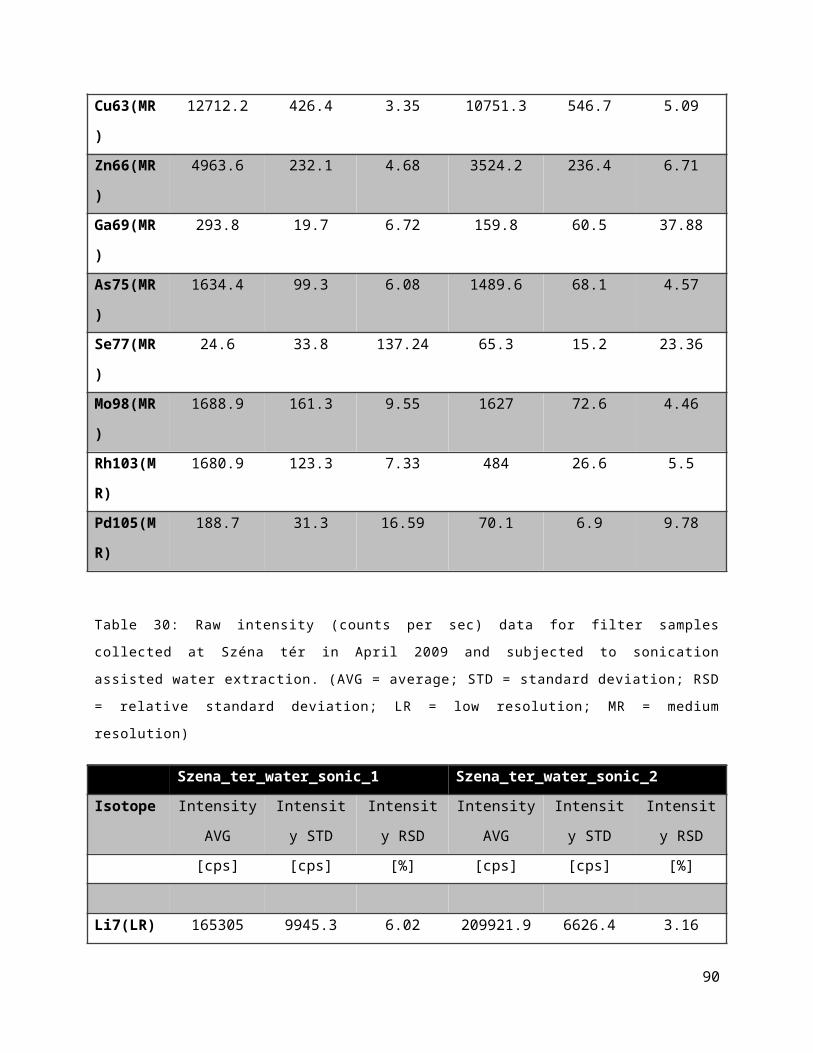
R)

In115(LR

)

6397519

6.7

444250

.2

0.69 6439679

1.5

996548

.6

1.55 6465907

8.6

906224

.9

1.4

Pt195(LR

)

8082 92.9 1.15 7185.1 117.2 1.63 3174.8 94.1 2.96

V51(MR) 3056.1 162.5 5.32 3251.2 126.2 3.88 2579.3 105.5 4.09

Cr52(MR

)

33923.3 1000.3 2.95 36115 1301.2 3.6 30987.3 1209.2 3.9

Mn55(M

R)

18330.5 835.5 4.56 18227.4 457.3 2.51 18052.9 210.7 1.17

Fe57(MR

)

12907.2 193.7 1.5 12357.4 163.5 1.32 11062 219.7 1.99

Co59(MR

)

140363.8 4002 2.85 14485.5 238.7 1.65 4861.3 115.1 2.37

Ni60(MR

)

17747.3 198.1 1.12 11612.8 407.2 3.51 13186.2 444.3 3.37

Cu63(MR

)

37944.7 240.9 0.63 32144.4 585.1 1.82 32006.9 742.1 2.32

Zn66(MR

)

106241.7 2485.9 2.34 214574 4185.8 1.95 84659.6 3517.1 4.15

Ga69(M

R)

1061.4 94.5 8.91 1122.1 84.7 7.55 1083.5 78.6 7.25

As75(MR

)

144401.1 6592.9 4.57 144795.8 4689.4 3.24 111461.8 2876 2.58

Se77(MR

)

73315.9 3148.2 4.29 73762.6 2704.5 3.67 60435.7 2352.2 3.89

Mo98(M

R)

992.4 111.4 11.22 1411.3 103.9 7.36 1642.2 73 4.45

Rh103(M

R)

1543.1 33.3 2.16 1340.6 22.4 1.67 729.3 30.2 4.14

90

Pd105(M

R)

480.7 34.6 7.2 429.2 14.5 3.37 367.9 21.9 5.94

In115(M

R)

4955110.

1

47774.

2

0.96 4962193.

1

51310.

7

1.03 4826800.

8

71956.

8

1.49

Table 47: Raw intensity (counts per sec) data for filter samples collected at Széna tér in May 2009

and subjected to microwave assisted digestion. (AVG = average; STD = standard deviation; RSD =

relative standard deviation; LR = low resolution; MR = medium resolution)

Szena_ter_acid_1 Szena_ter_acid_2

Isotope Intensity

AVG

Intensity

STD

Intensity

RSD

Intensity

AVG

Intensity

STD

Intensity

RSD

[cps] [cps] [%] [cps] [cps] [%]

Li7(LR) 113548.8 3055.6 2.69 115745.3 2160.1 1.87

Be9(LR) 5854.6 153.5 2.62 3284.2 189.3 5.76

Rb85(LR) 378010.5 24679.9 6.53 420497 1587.5 0.38

Sr88(LR) 1630521.2 18577.6 1.14 1500356.5 37241.1 2.48

Sn120(LR) 688231.9 11030.1 1.6 751088 7958.2 1.06

Sb121(LR) 355656.9 5995 1.69 378306.1 9313.2 2.46

Te128(LR) 2558.3 114.9 4.49 2513.5 44.2 1.76

Au197(LR) 9587048.2 39143.2 0.41 8957513.1 100851.8 1.13

Tl205(LR) 49644.3 1254.7 2.53 47665.2 1252.4 2.63

Pb208(LR) 3886578.8 61584.2 1.58 4274291.4 43636.3 1.02

Bi209(LR) 149999.1 3807 2.54 219767.4 8817.6 4.01

U238(LR) 86173.9 8295.4 9.63 81776.8 1331.7 1.63

Ag109(LR) 52477.9 1302.9 2.48 43069.9 392.1 0.91

Cd114(LR) 78672.7 1805.1 2.29 74504.6 843.8 1.13

In115(LR) 65370749.8 602463.2 0.92 63998573 1038905.1 1.62

Pt195(LR) 15641.9 226.3 1.45 3522.7 89 2.53

V51(MR) 34119.6 1399.5 4.1 36319 2340.7 6.44

Cr52(MR) 121867.3 5366.6 4.4 109361.7 1469.1 1.34

91

Mn55(MR) 573867.8 17775.7 3.1 620832.5 8837.8 1.42

Fe57(MR) 488006.2 13487.3 2.76 576369.8 4653.2 0.81

Co59(MR) 335118.8 6247.1 1.86 57761.4 2712.6 4.7

Ni60(MR) 22234 660.7 2.97 22038 731 3.32

Cu63(MR) 319789.4 11746.8 3.67 379692.6 4508.1 1.19

Zn66(MR) 151175.2 2659.5 1.76 371110.8 1354.1 0.36

Ga69(MR) 4214.6 205.1 4.87 4064 74 1.82

As75(MR) 87437.8 5744.2 6.57 72120.3 6010 8.33

Se77(MR) 43420.3 2447.4 5.64 38357.3 565.1 1.47

Mo98(MR) 8931.1 673.2 7.54 9989.7 112.7 1.13

Rh103(MR) 2575.1 100.4 3.9 745 39.8 5.35

Pd105(MR) 1086.9 37.8 3.48 875.4 37.2 4.25

In115(MR) 4330265.9 146124.5 3.37 4271669.3 82290.7 1.93

Table 48: Raw intensity (counts per sec) data for filter samples collected at Gilice tér in May 2009

and subjected to microwave assisted digestion. (AVG = average; STD = standard deviation; RSD =

relative standard deviation; LR = low resolution; MR = medium resolution)

Gilice_ter_acid_1 Gilice_ter_acid_2

Isotope Intensity

AVG

Intensity

STD

Intensity

RSD

Intensity

AVG

Intensity

STD

Intensity

RSD

[cps] [cps] [%] [cps] [cps] [%]

Li7(LR) 74556.1 2948 3.95 75735.6 5548.9 7.33

Be9(LR) 3221.3 91.5 2.84 3337.6 132.8 3.98

Rb85(LR) 364430.4 3281.1 0.9 607352.4 4538.3 0.75

Sr88(LR) 1217379.9 8338.6 0.68 1478804.3 8109.3 0.55

Sn120(LR) 465914.6 2912.8 0.63 531944.7 1659 0.31

Sb121(LR) 243135.6 752.4 0.31 276456.2 3845.4 1.39

Te128(LR) 2459.6 68.3 2.78 2592.8 91.5 3.53

Au197(LR) 9122457.2 94447.4 1.04 9062060.3 104386.3 1.15

92

Tl205(LR) 47126.7 1225.6 2.6 50315.8 150.5 0.3

Pb208(LR) 4927928.8 91502.8 1.86 5972035.1 118820.9 1.99

Bi209(LR) 126861.3 6045 4.77 309806.4 5001.9 1.61

U238(LR) 78717 3078.1 3.91 82431.7 1193.7 1.45

Ag109(LR) 112367 4637.9 4.13 65756.1 3095.9 4.71

Cd114(LR) 71829.7 3648.9 5.08 87450.1 1075.5 1.23

In115(LR) 63931211.4 281444.6 0.44 63630304.2 581841.2 0.91

Pt195(LR) 3257.4 51.8 1.59 3046.6 45.2 1.48

V51(MR) 33766.4 1103.3 3.27 42801.9 935.8 2.19

Cr52(MR) 56880.2 1207.7 2.12 76182.7 529.6 0.7

Mn55(MR) 307027.6 8655.6 2.82 383552.6 7895.2 2.06

Fe57(MR) 219968.1 2086.9 0.95 260203.8 2359.1 0.91

Co59(MR) 7799.3 392 5.03 9744.4 144.9 1.49

Ni60(MR) 17039.5 511.3 3 32169 693.1 2.15

Cu63(MR) 174763.8 1931.8 1.11 258205.8 2228.5 0.86

Zn66(MR) 240199.9 8662.1 3.61 242634.3 14194.7 5.85

Ga69(MR) 3763.5 173.5 4.61 4690.6 328.4 7

As75(MR) 73666.3 2250.2 3.05 55489.3 3701.1 6.67

Se77(MR) 36756.2 1301.8 3.54 28708.6 712.7 2.48

Mo98(MR) 8485.8 260.1 3.07 5866.3 186.1 3.17

Rh103(MR) 758.4 38.8 5.12 726.6 32.8 4.51

Pd105(MR) 759.1 30.6 4.03 1002.8 46.6 4.64

In115(MR) 4261510.4 82583.3 1.94 3919297 272489.6 6.95

Table 49: Raw intensity (counts per sec) data for filter samples collected at the incinerator located

in Káposztásmegyer in May 2009 and subjected to microwave assisted digestion. (AVG = average;

STD = standard deviation; RSD = relative standard deviation; LR = low resolution; MR = medium

resolution)

Kapmegyer_acid_1 Kapmegyer_acid_2

Isotope Intensity Intensity Intensity Intensity Intensity Intensity

93

AVG STD RSD AVG STD RSD

[cps] [cps] [%] [cps] [cps] [%]

Li7(LR) 145205.5 4249 2.93 143404.2 2352.3 1.64

Be9(LR) 4469.6 67.9 1.52 4155.8 70.9 1.71

Rb85(LR) 1167639.9 10454.2 0.9 1167027.7 23700.3 2.03

Sr88(LR) 2613154.9 36750.5 1.41 2486656.8 109756 4.41

Sn120(LR) 520060.2 5079.4 0.98 575917.8 4988.2 0.87

Sb121(LR) 304044 2637.3 0.87 341623.9 3229.4 0.95

Te128(LR) 2519.1 101.1 4.01 2373.3 54.3 2.29

Au197(LR) 9843479.2 31045 0.32 8771486.3 311943.3 3.56

Tl205(LR) 50371.3 736.7 1.46 53187.5 1032.9 1.94

Pb208(LR) 5987700.8 133675.1 2.23 7316588.8 82109.7 1.12

Bi209(LR) 125504.6 1075.6 0.86 173127 2449.2 1.41

U238(LR) 99523.9 2518.8 2.53 97598.8 1294.6 1.33

Ag109(LR) 42528.1 570.1 1.34 107812.3 5394 5

Cd114(LR) 73827.5 725.8 0.98 81024.8 1379.6 1.7

In115(LR) 62369020.6 537691.1 0.86 62044888 625573.1 1.01

Pt195(LR) 3265.9 64.4 1.97 3144.9 42.3 1.34

V51(MR) 77527.8 3957.7 5.1 85670.9 2876 3.36

Cr52(MR) 108376.5 579.3 0.53 114842.6 3469.1 3.02

Mn55(MR) 852549.2 30097.8 3.53 969019.6 6502.4 0.67

Fe57(MR) 712742.6 10307 1.45 795306.3 7102.9 0.89

Co59(MR) 15169.1 389.6 2.57 16280 368.4 2.26

Ni60(MR) 21595.1 577 2.67 32654.7 1284.4 3.93

Cu63(MR) 295998.5 9304.4 3.14 333862.8 8048.8 2.41

Zn66(MR) 161565.5 6465.7 4 163074.2 3372 2.07

Ga69(MR) 9738.5 213.5 2.19 9699.3 449.8 4.64

As75(MR) 50575.2 1460.4 2.89 50962.5 2862.9 5.62

Se77(MR) 25430.6 644.8 2.54 25913.3 1105.6 4.27

Mo98(MR) 5647.8 167.4 2.96 6834.4 136.3 1.99

94

Rh103(MR) 729.7 39.4 5.4 757.3 24.5 3.24

Pd105(MR) 2962.5 80.9 2.73 3141.1 33.3 1.06

In115(MR) 3821830.7 121478.6 3.18 3901894.6 249027.4 6.38

Table 50: Raw intensity (counts per sec) data for filter blanks, subjected to microwave assisted

digestion for the sampling period of June 2009. (AVG = average; STD = standard deviation; RSD =

relative standard deviation; LR = low resolution; MR = medium resolution)

filter_blank_acid_1 filter_blank_acid_2

Isotope Intensity

AVG

Intensity

STD

Intensity

RSD

Intensity

AVG

Intensity

STD

Intensity

RSD

[cps] [cps] [%] [cps] [cps] [%]

Li7(LR) 51206.3 1910.4 3.73 49364.3 3399.6 6.89

Be9(LR) 2936 139.3 4.74 2744.7 231.6 8.44

Rb85(LR) 50577.5 550.6 1.09 57902.3 1626.6 2.81

Sr88(LR) 432590.9 3620.1 0.84 479058.2 6396.7 1.34

Sn120(LR) 127785.5 176.9 0.14 129103.4 471.9 0.37

Sb121(LR) 61097.5 392.1 0.64 60611.1 1091.1 1.8

Te128(LR) 1225.2 58.7 4.79 1176.6 50.4 4.28

Au197(LR) 9787283.3 43117 0.44 9880273 214644.7 2.17

Tl205(LR) 24676.3 502.4 2.04 26256.5 258.5 0.98

Pb208(LR) 250287.2 3116.5 1.25 260921.8 3373.3 1.29

Bi209(LR) 33495.4 1519.4 4.54 33483.1 1187.4 3.55

U238(LR) 69415.8 3293.3 4.74 70332.3 2718.9 3.87

Ag109(LR) 10561.9 475.3 4.5 9407.5 162.7 1.73

Cd114(LR) 12288.9 261.8 2.13 11323.5 509.7 4.5

In115(LR) 63311087 496277 0.78 61028249 635506.9 1.04

Pt195(LR) 1677.8 54.5 3.25 1714.5 33.5 1.95

V51(MR) 1693.1 74.7 4.41 1699.5 63.1 3.72

Cr52(MR) 22840.3 743.4 3.25 20224.2 800.6 3.96

Mn55(MR) 10955 455.8 4.16 12132.2 144.7 1.19

95

Fe57(MR) 9177.6 102.5 1.12 8153.9 277.7 3.41

Co59(MR) 1505.2 50.8 3.38 2048.2 69 3.37

Ni60(MR) 15791.6 812.9 5.15 13950.5 463.4 3.32

Cu63(MR) 34510.2 1425.6 4.13 29331 581.3 1.98

Zn66(MR) 27516.7 134.6 0.49 32774.2 811.5 2.48

Ga69(MR) 789.2 51.4 6.51 936 51.6 5.51

As75(MR) 376858 12180.2 3.23 330261.3 11191.3 3.39

Se77(MR) 122215.5 3268.8 2.67 105453.9 3021.4 2.87

Mo98(MR) 653.8 60.8 9.29 783.9 82.1 10.48

Rh103(MR) 534.5 22.1 4.13 519 11.8 2.27

Pd105(MR) 231.3 15.3 6.6 297.5 15.4 5.19

In115(MR) 4124117 40704.3 0.99 4064877 195914.8 4.82

Table 51: Raw intensity (counts per sec) data for filter samples collected at Széna tér in June 2009

and subjected to microwave assisted digestion. (AVG = average; STD = standard deviation; RSD =

relative standard deviation; LR = low resolution; MR = medium resolution)

Szena_ter_acid_1 Szena_ter_acid_2

Isotope Intensity

AVG

Intensity

STD

Intensity

RSD

Intensity

AVG

Intensity

STD

Intensity

RSD

[cps] [cps] [%] [cps] [cps] [%]

Li7(LR) 64148.7 4172 6.5 70877.5 4051 5.72

Be9(LR) 2894.9 141.4 4.88 2825.4 207.6 7.35

Rb85(LR) 269525.9 13464.9 5 320236.5 4846.9 1.51

Sr88(LR) 1086279.6 19122.6 1.76 1188252.9 63035.3 5.3

Sn120(LR) 602595.2 13432.4 2.23 709505.7 5152.1 0.73

Sb121(LR) 283806.7 4939.6 1.74 333151 2241.8 0.67

Te128(LR) 1915.9 24.6 1.29 2024.4 86.2 4.26

Au197(LR) 9587067.7 88379.3 0.92 9269755.8 122946.8 1.33

Tl205(LR) 40631.9 243.4 0.6 44090.2 759.3 1.72

96

Pb208(LR) 3987068.3 90852.8 2.28 4787417.8 64236.4 1.34

Bi209(LR) 137219.5 2810.5 2.05 169150.3 920.8 0.54

U238(LR) 76764.5 4594 5.98 76662 1115.4 1.45

Ag109(LR) 29734.6 1017.8 3.42 96360 2969.3 3.08

Cd114(LR) 58914.3 1906.2 3.24 66752.2 1331 1.99

In115(LR) 58569520.2 2246609 3.84 59620268.2 255616.1 0.43

Pt195(LR) 2099.2 55.5 2.64 2064.8 44.4 2.15

V51(MR) 28452.5 1404.5 4.94 35088.1 579.5 1.65

Cr52(MR) 78224 5379.1 6.88 99406.7 1350.4 1.36

Mn55(MR) 308783.7 9030 2.92 398269.2 3009.7 0.76

Fe57(MR) 340778.1 3071 0.9 424530.1 4427.9 1.04

Co59(MR) 4498 292.1 6.49 6896.6 130.5 1.89

Ni60(MR) 18547.9 545.5 2.94 21033.3 541.7 2.58

Cu63(MR) 279949.6 7695.8 2.75 345353.4 1424.7 0.41

Zn66(MR) 107523.9 993.2 0.92 128442.9 943.3 0.73

Ga69(MR) 2732.8 172.3 6.3 3121.4 161.1 5.16

As75(MR) 286420 6581.9 2.3 289473 6306.7 2.18

Se77(MR) 89855.1 3927.3 4.37 90086.7 3878.7 4.31

Mo98(MR) 7059.3 298.7 4.23 8579 551.5 6.43

Rh103(MR) 551.8 14.9 2.7 545.7 11.3 2.08

Pd105(MR) 555.4 29.2 5.26 612.3 6.1 0.99

In115(MR) 3947093.7 185335.2 4.7 4050175.8 79978.5 1.97

Table 52: Raw intensity (counts per sec) data for filter samples collected at Gilice tér in June 2009

and subjected to microwave assisted digestion. (AVG = average; STD = standard deviation; RSD =

relative standard deviation; LR = low resolution; MR = medium resolution)

Gilice_ter_acid_1 Gilice_ter_acid_2

Isotope Intensity

AVG

Intensity

STD

Intensity

RSD

Intensity

AVG

Intensity

STD

Intensity

RSD

[cps] [cps] [%] [cps] [cps] [%]

97

Li7(LR) 53979.6 1542.3 2.86 56033.5 1293.5 2.31

Be9(LR) 2653.3 137.4 5.18 2763.9 186.6 6.75

Rb85(LR) 238066.7 2300.4 0.97 255333.1 4625.6 1.81

Sr88(LR) 793205.5 4665.5 0.59 821890 12908.5 1.57

Sn120(LR) 369248.6 11246.2 3.05 388550.7 2196.1 0.57

Sb121(LR) 201576.5 2050.5 1.02 228506.1 5011.4 2.19

Te128(LR) 2062.5 102.5 4.97 2161.5 75.7 3.5

Au197(LR) 9089571.3 319520.7 3.52 9090486 254756.6 2.8

Tl205(LR) 47688 719 1.51 54532.2 771.5 1.41

Pb208(LR) 3830945.6 87743.2 2.29 4311910.1 50342.6 1.17

Bi209(LR) 77617.3 970.7 1.25 82945.6 1516.6 1.83

U238(LR) 71227.9 6088.7 8.55 73359.1 1431.4 1.95

Ag109(LR) 24593.8 535.9 2.18 30886.2 620.2 2.01

Cd114(LR) 59100.5 1334.8 2.26 63652.3 284.8 0.45

In115(LR) 59639505.2 474089.3 0.79 59634499.5 244602.1 0.41

Pt195(LR) 1715.4 54.1 3.16 1708 67.6 3.96

V51(MR) 26584.2 355.9 1.34 29606.9 1293.4 4.37

Cr52(MR) 56584 1127.7 1.99 51853.5 1772 3.42

Mn55(MR) 207219.5 3257.1 1.57 231010.2 6263.3 2.71

Fe57(MR) 140823.2 1368.8 0.97 165188.3 1110.9 0.67

Co59(MR) 6604.3 258.8 3.92 6058.4 74 1.22

Ni60(MR) 20212.8 292.1 1.45 23583 656.1 2.78

Cu63(MR) 139049.3 3269.3 2.35 150179.2 4673 3.11

Zn66(MR) 101229.9 1598.2 1.58 112498.1 493.9 0.44

Ga69(MR) 1979.3 147.6 7.46 2308.6 116.7 5.06

As75(MR) 294128.3 11848.4 4.03 328663.7 6903.1 2.1

Se77(MR) 93016.9 3476.7 3.74 105517.5 1647 1.56

Mo98(MR) 3800 170.2 4.48 3935.6 282.7 7.18

Rh103(MR) 491.5 21.2 4.32 508.4 32.1 6.32

98

Pd105(MR) 377.1 15.4 4.09 437.2 31.6 7.22

In115(MR) 4025626.6 159903.9 3.97 4171355.2 68072.2 1.63

Table 53: Raw intensity (counts per sec) data for filter samples collected at the incinerator located

in Káposztásmegyer in June 2009 and subjected to microwave assisted digestion. (AVG = average;

STD = standard deviation; RSD = relative standard deviation; LR = low resolution; MR = medium

resolution)

Kaposztasmegyer_acid_1 Kaposztasmegyer_acid_2

Isotope Intensity

AVG

Intensity

STD

Intensity

RSD

Intensity

AVG

Intensity

STD

Intensity

RSD

[cps] [cps] [%] [cps] [cps] [%]

Li7(LR) 59226.6 2109.8 3.56 65725.5 1206.3 1.84

Be9(LR) 2735.7 218.2 7.98 2910.8 155.5 5.34

Rb85(LR) 266643.3 2582.7 0.97 298101.8 7630.6 2.56

Sr88(LR) 828269.9 4735.9 0.57 863475.2 4939.2 0.57

Sn120(LR) 388008.7 3450.3 0.89 403744.7 9027.4 2.24

Sb121(LR) 234724.8 1457.7 0.62 233889 774.1 0.33

Te128(LR) 2142.5 102 4.76 2109.5 52.6 2.49

Au197(LR) 9375053 61147.5 0.65 9232720.1 69245.9 0.75

Tl205(LR) 48024 447.4 0.93 47708.4 945.5 1.98

Pb208(LR) 4313147.5 32731.7 0.76 4377982.5 38589.8 0.88

Bi209(LR) 90576 893.4 0.99 87187.4 1591.6 1.83

U238(LR) 74333.2 5156 6.94 75219.2 1235.7 1.64

Ag109(LR) 28091.4 259.2 0.92 34796.5 314.7 0.9

Cd114(LR) 62028.2 2582.9 4.16 63755.9 1251.5 1.96

In115(LR) 59436325.2 1180398 1.99 59111494 262903.1 0.44

Pt195(LR) 1741.5 38.9 2.23 1750.9 37.7 2.15

V51(MR) 31970.1 886 2.77 34551 692.7 2

Cr52(MR) 70955.4 1369.2 1.93 55961.8 609.1 1.09

Mn55(MR) 230526.2 9698.6 4.21 261330.2 6588.1 2.52

99

Fe57(MR) 183336.9 1313.3 0.72 202469.2 812 0.4

Co59(MR) 5980.3 319.8 5.35 6639.2 310.2 4.67

Ni60(MR) 29708.9 497.7 1.68 23059 592.2 2.57

Cu63(MR) 199768.7 1651.8 0.83 191292.9 2535.1 1.33

Zn66(MR) 119588.8 2633.2 2.2 110581.7 3993.1 3.61

Ga69(MR) 2121.7 151.3 7.13 2402.6 44.1 1.83

As75(MR) 309954.5 5076.4 1.64 324027.4 12365 3.82

Se77(MR) 98420.5 2284.8 2.32 107360.9 834 0.78

Mo98(MR) 4884 172.2 3.53 5276.7 134.7 2.55

Rh103(MR) 506.2 21.1 4.17 489.1 29.1 5.96

Pd105(MR) 455.7 40.1 8.79 568.3 52.9 9.3

In115(MR) 4078047.2 133110.5 3.26 4076401.4 91195 2.24

100