characterization of the spatial and temporal variations of ... · groundwater discharge using...

Characterization of the Spatial and Temporal Variations of Submarine

Groundwater Discharge Using Electrical Resistivity and Seepage Measurements

A Dissertation Presented

by

Josephine Miryam Kalyanie Durand

to

The Graduate School

in Partial Fulfillment of the

Requirements

for the Degree of

Doctor of Philosophy

in

Geosciences

(Hydrogeology)

Stony Brook University

August 2014

Copyright by

Josephine M. K. Durand

2014

ii


The Graduate School


We, the dissertation committee for the above candidate for the

Doctor of Philosophy degree, hereby recommend

acceptance of this dissertation.

Teng-fong Wong –Dissertation Advisor

Professor, Geosciences

Daniel Davis - Chairperson of Defense

Professor and Chair, Geosciences

Gilbert Hanson

Distinguished Service Professor, Geosciences

Henry Bokuniewicz

Distinguished Service Professor, School of Marine and Atmospheric Sciences

Harold Walker

Professor and Civil Engineering Program Director, Stony Brook University

This dissertation is accepted by the Graduate School

Charles Taber

Dean of the Graduate School

iii

Abstract of the Dissertation

Characterization of the Spatial and Temporal Variations of Submarine Groundwater

Discharge Using Electrical Resistivity and Seepage Measurements

by


Doctor of Philosophy

in

Geosciences

(Hydrogeology)


2014

Submarine groundwater discharge (SGD) encompasses all fluids crossing the

sediment/ocean interface, regardless of their origin, composition or driving forces. SGD provides

a pathway for terrestrial contaminants that can significantly impact coastal ecosystems.

Overexploitation of groundwater resources can decrease SGD which favors seawater intrusion at

depth. Understanding SGD is therefore crucial for water quality and resource management.

Quantifying SGD is challenging due to its diffuse and heterogeneous nature, in addition to

significant spatio-temporal variations at multiple scales.

In this thesis, an integrated approach combining electrical resistivity (ER) surveys,

conductivity and temperature point measurements, seepage rates using manual and ultrasonic

seepage meters, and pore fluid salinities was used to characterize SGD spatio-temporal variations

and their implications for contaminant transport at several locations on Long Island, NY.

The influence of surficial sediments on SGD distribution was investigated in Stony Brook

Harbor. A low-permeability mud layer, actively depositing in the harbor, limits SGD at the

shoreline, prevents mixing with seawater and channels a significant volume of freshwater

offshore. SGD measured at locations without mud is high and indicates significant mixing

iv

between porewater and seawater. A 2D steady-state density-difference numerical model of the

harbor was developed using SEAWAT and was validated by our field observations.

Temporal variations of SGD due to semi-diurnal tidal forcing were studied in West Neck

Bay, Shelter Island, using a 12-hr time-lapse ER survey together with continuous salinity and

seepage measurements in the intertidal zone. The observed dynamic patterns of groundwater flux

and salinity distribution disagree with published standard transient state numerical models,

suggesting the need for developing more specific models of non-homogeneous anisotropic

aquifers.

SGD distribution and composition were characterized in Forge River, a tidal river that

experiences chronic hypoxia due to nitrogen contamination. We found that nitrogen speciation

and concentration are linked to different SGD regimes. Near shore sandy zones with high SGD

show little nitrate reduction and constitute the major source of nitrogen input to surface waters.

Offshore areas rich in silt and organic matter exhibit low SGD and higher denitrification.

Dredging activities have altered the sediment distribution and subsequently have created

preferential flow paths focusing freshwater discharge into the center of the river.

For Stony Brook Harbor study presented in chapter 2, I acquired, processed and

interpreted the electrical resistivity and seepage meter data. Caitlin Young helped during

collection of manual seepage data and Joseph Tamborski provided assistance for the mud

mapping. The piezometers were installed for a parallel study focusing on denitrification but

allowed me to collect and use porewater salinity measurements. Teng-fong Wong and Gilbert

Hanson helped with the preparation of the manuscript. Design, simulations and result

interpretation of the numerical model presented in chapter 3 were done without external

contribution. Data presented in chapter 4 were collected with the help of Neal Stark and Jonathan

Wanlass. I performed the processing, analysis and data interpretation. Teng-fong Wong assisted

with the preparation of the manuscript. For chapter 5, Neal Stark assisted with the electrical

resistivity data acquisition and collected all the water samples in Forge River. Ronald Paulsen

provided help with the preparation of the report.

v

Dedication Page

To the Earth, for being:

a never-ending source of wonders,

a spring of breath-taking beauty

and a constant provider of infinite mysteries.

À Dany, pour tout et plus encore…

vi

Frontispiece

Salinity and flow rates measurements from manual seepage meters in Stony Brook Harbor, NY.

The meters A, B and C were placed at 1, 20 and 22 m offshore of the low tide mark, respectively.

Each square represents a sampling interval: the base shows the sampling duration in hours, the

square height the seepage rate in cm/d and the color the salinity. The blue dotted line indicates

the tidal level, in m. Note the different scale for the seepage meter C.

vii

Table of Contents

Table of Content………………………………………………………………………………vii

List of Figures……………………………………………………………………………………x

List of Tables…………………………………………………………………………………xiv

List of Abbreviations……………………………………………………………………………xv

Acknowledgments……………………………………………………………………………xvi

Publications……………………………………………………………………………………xvii

Chapter 1: Introduction………………………………………………………………………1

Introduction……………………………………………………………………………1

References……………………………………………………………………………..6

Chapter 2: Effect of a surficial low permeability mud layer on submarine groundwater

discharge: a case study in Stony Brook Harbor, New York………………………………11

Abstract……………………………………………………………………………..…11

Introduction……………………………………………………………………………12

Study site…………………….……………………………………………………...…14

Methods……………………………………………………………………………..…15

Trident……………………………………………………………………..…15

Electrical resistivity data acquisition and inversion…………….……………16

Seepage meters………………………………………………………………17

Piezometers………………………………………………………………...…18

Mud layer mapping and sediment core analysis………………………….…..18

Results…………………………………………………………………………………19

Stony Brook Harbor bulk conductivity and temperature anomalies………19

Electrical conductivity………………………………………………….…….20

Piezometer transects…………………………………………………………21

Seepage measurements………………………………………………………23

Ultrasonic seepage meters.……………………………………………23

Manual seepage meters.……………………………………………….24

Sediment core analysis……………………………………………………….25

Discussion……………………………………………………………………………..25

Conceptual models…………………………………………………………...25

Stony Brook Harbor SGD……………………………………………………26

Implications for water and nutrients budgets…………………….…………28

Sources of error………………………………………………………………29

Conclusion……………………………………………………………………………..31

Acknowledgments…………………………………………………………………..…31

References……………………………………………………………………………..33

Figures and captions ……………………………………………………………….…39

viii

Chapter 3: Groundwater flow and solute transport modeling of a coastal unconfined

sandy aquifer: application to Stony Brook Harbor…………………………………………49

Abstract……………………………………………………………………………..…49

Introduction……………………………………………………………………………50

Mathematical model…………………………………………………………………..52

Conceptual model and implementation………………………………………………54

Stony Brook model description and parameters………………………………………56

Model results…………………………………………………………………………..57

Conclusion…………………………………………………………………………..…59

References…………………………………………………………………………..…61

Tables……………………………………………………………………………….…65

Figures and captions…………………………………………………………………..66

Chapter 4: Time-lapse electrical resistivity survey of the intertidal zone and implications

for submarine ground water discharge……………………………………………………..70

Abstract………………………………………………………………………..………70

Introduction……………………………………………………………………………71

Study Site………………………………………………………………………..…….72

Methods……………………………………………………………………….…….…73

Electrical resistivity survey acquisition and processing………………..…..73

Seepage meters………………………………………………………….……75

Trident probe…………………………………………………………………76

Salinity measurements…………………………………………………..……76

Results…………………………………………………………………………………77

Electrical resistivity surveys and Trident probe………………………….…77

SGD in the intertidal zone: manual seepage meters…………………………80

SGD in the subtidal zone: ultrasonic seepage meters………………………81

Discussion………………………………………………………………………..……82

Comparison with other studies: SGD rates …………………………………82

Interpretation of SGD composition ...………………………………………..83

Impact of sediment heterogeneities on SGD………………………………85

Interpretation of ER time-lapse survey……………………………………85

Conclusion……………………………………………………………………………86

References……………………………………………………………………………88

Tables…………………………………………………………….…………………93

Figures and captions…………………………………………………………………94

Chapter 5: Nutrient loading associated with submarine groundwater discharge in Forge

River…………………………………………………………………………………………104

Abstract………………………………………………………………………………104

Introduction…………………………………………………………………………..105

Background…………………………………………………………………105

Objective of the project……………………………………………………106

Methodology: equipment and field procedure……………………………………….107

Equipment…………………………………………………………………...107

Trident probe………………………………………………………...108

Supersting resistivity system………………………………………...109

ix

Ultrasonic seepage meter……………………………………………109

Field procedure……………………………………………………………...110

Trident probe………………………………………………………...110

Supersting resistivity system and EarthImager2D …………………111

Ultrasonic seepage meter……………………………………………112

Water sampling……………………………………………………113

Well design…………………………………………………113

Nutrient analysis……………………………………………...115

In situ pore water analysis……………………………………116

Results………………………………………………………………………………116

Trident mapping and pore water conductivity sections……………………116

Electrical resistivity surveys………………………………………………121

Ultrasonic seepage meter……………………………………………………124

Well profiles………………………………………………………………125

Results of nutrient analysis for transect FR1………………………125

Results of nutrient analysis for transect FR2………………………131

Results of nutrient analysis for inland wells………………………135

Conclusion……………………………………………………………………………136

References……………………………………………………………………………140

Appendices…………………………………………………………………………142

Appendix 1: Trident values associated with the electrical resistivity surveys at

FR1 and FR2 in Forge River……………………………………………142

Appendix 2: Trident results associated with the wells for transects FR1 and

FR2, in Forge River…………………………………………………………143

Appendix 3: Piezometer wells description at FR1 and FR2, in Forge

River………………………………………………………………………144

Appendix 4: Results of pore water analysis for transect FR1 in Forge

River………………………………………………………………………..145

Appendix 5: Results of pore water analysis for transect FR2 in Forge

River………………………………………………………………………146

Chapter 6: Conclusion and path forward…………………………………………………147

Conclusion……………………………………………………………………………147

Path forward………………………………………………………………………….149

References………………………………………………………………………...151

List of References……………………………………………………………………………153

x

List of Figures

Figure 1: (a) Site map of Stony Brook Harbor and inclusion of general location. (b) Cross

section of relative positions of the different measurements at site 1. (c) Cross section

of relative positions of the different measurements at site 2. The vertical black dotted

lines indicate the piezometer wells. The number following the P indicates the site

and the number after the hyphen, the distance from the first piezometer. The grey

dots show the positions of the manual seepage meters. The stars, F, indicate the

positions of the ultrasonic seepage meter funnels. The electrical resistivity transects,

T, are plotted as solid or dotted lines with black inverted triangles. The black cross

(x) indicate the position of the mean lower level of water (MLLW). The sections are

presented with 5x vertical exaggeration ………………………………………...39

Figure 2: Site map of the Trident probe transects realized between 3/28/11 and 4/11/11 across

Stony Brook Harbor. (a) Bulk temperature of sediments at 60 cm depth, in °C. (b)

Surface water temperature, in °C. (c) Temperature difference between sediments and

surface water……………………………………………………………………….40

Figure 3: Inverted conductivity sections at site 1 (a) and site 2 (b), in μS/cm. The black dotted

line indicates the position of the cable and the electrodes, the black crosses (x)

indicate the position of the MLLW, the high tide marks would be landward of both

profiles. Colors are plotted on a log scale. RMS values are 6.03% and 6.13% for

sections at site1 and 2, respectively…………………………………………………41

Figure 4: Inverted conductivity section of the double-cable transect T1-2 at low tide at site 1.

Conductivities are plotted on a log scale, in μS/cm. The black dotted line indicates

the position of the cable with the electrodes. The MLLW mark was located a couple

of meters landward of the profile. The RMS value is 7.68%..............................42

Figure 5: Comparison of piezometer pore water conductivities and inverted conductivity

sections at sites 1 (a) and 2 (b). Conductivities are plotted on a log scale.

Topography is indicated with a black solid line…………………………………43

Figure 6: Salinity measurements for the piezometer transects at site 1 (a) and site 2 (b). The

dots show the locations of porewater samples. Colors indicate the value of salinity.

The cross (x) marks the position of the mean lower level of water (MLLW). The

high tide marks would be a couple of meters landward of the profiles………44

Figure 7: Four-point moving average of specific discharge measurements by the ultrasonic

seepage meters (cm/d), at site 1: funnel 1 (a) implanted at 25m offshore of the

MLLW from 7/22/11 to 7/29/11, and site 2: funnel 2 (b) implanted at 30m offshore

of the MLLW from 5/19/11 to 5/26/11, funnel 3 (c) implanted at 40m offshore of the

MLLW from 7/22/11 to 7/29/11 and funnel 4 (d), implanted at 45m offshore of the

MLLW from 7/22/11 to 7/29/11. The grey dotted lines indicate the tidal level,

xi

(m)…………………………………………………………………………………..45

Figure 8: Salinity and specific discharge measurements from the manual seepage meters at site

1. Seepage meters A, B and C were placed at 1, 20 and 22 m offshore of the low tide

mark, respectively. Each rectangle represents a sampling bag: the base shows the

sampling duration in hours, the height the seepage rate in cm/d and the color the

salinity. The blue dotted line indicates the tidal level, in m. Note the different scale

for the seepage meter C……………………………………………………………..46

Figure 9: Interpolated map of the mud thickness in the southern portion of Stony Brook

Harbor, in cm, and relative locations of sites 1 and 2………………………………47

Figure 10: Conceptual model of groundwater fluxes in the absence (a) or presence (b) of a mud

cap. HT and LT indicate the high tide and low tide marks, respectively. The cap

limits the vertical flow and thus controls the extent of infiltration, mixing and

circulation of seawater………………………………………………………………48

Figure 11: Grid mesh of Stony Brook harbor numerical SEAWAT model. The mud layer starts

at x ~ 90 m, and appears as a bold line at the top of the sediments……………66

Figure 12: Boundary conditions of a 2D density-difference numerical model of an unconfined

coastal aquifer with a sloping beach……………………………………………..….67

Figure 13: Equipotential distribution (in m) for Stony Brook Harbor steady state model without

(a) and with (b) the low-permeability mud layer, shown as the bolded black line…68

Figure 14: Salinity distribution for Stony Brook Harbor steady state model without (a) and with

(b) the low-permeability the mud layer, plotted as a black bold line……………….69

Figure 15: Location map of Shelter Island and position of study site……………………...…..94

Figure 16: Experimental setting in West Neck Bay. (a) Relative positions of data sampling

locations. The position of the first electrode is taken as origin of the framework. (b)

Time-lapse ER surveys and associated tidal level…………………………………..95

Figure 17: Comparison between the inverted conductivity section and the Trident probe

conductivity measurements (filled in circles). The resistivity cable is shown as a

solid black line. The black crosses indicate the position of the high tide (HT) and low

tide (LT) marks. Conductivities are plotted on a log scale…………………………96

Figure 18: Comparison of inverted resistivity sections obtained from 3 different initial models:

the apparent resistivity pseudosection (a), the average apparent resistivity

homogeneous model (b) and a custom homogeneous resistivity model (c).

Resistivities, in ohm-m, are plotted on a log scale………………………………….97

xii

Figure 19: Inverted conductivity sections of time lapse survey, profiles A to F. Bulk

conductivity is plotted on a log scale in μS/cm. High tide and low tide marks are

indicated by black crosses (x), the dashed line shows the water level……………...98

Figure 20: Inverted conductivity sections of time lapse survey, profiles G to L. Bulk

conductivity is plotted on a log scale in μS/cm. High tide and low tide marks are

indicated by black crosses (x), the dashed line shows the water level……………...99

Figure 21: Average conductivity sections for the high tide (a) and low tide (b) end-members,

and for the phase-averaged profile (c), in μS/cm. Conductivities are plotted on a log

scale………………………………………………………………………………..100

Figure 22: Seepage rates and salinity measured with the manual seepage meters M1 (a) and M2

(b) in the intertidal zone…………………………………………………………101

Figure 23: Salinities and freshwater content (%) measured in the manual seepage collection

bags (a) and computed for SGD entering the seepage meters (b)…………………102

Figure 24: Seepage rates measured with the ultrasonic seepage meters U1 (a) and U2 (b), in

cm/d (black solid line). The relative tidal level is plotted with a grey dashed line;

salinity, is plotted in grey with square markers……………………………………103

Figure 25: Site map with general location inclusion in upper right corner. The study zone

includes two transects in the Forge River and another in Wills Creek…………107

Figure 26: Site map showing Trident point locations associated with the wells, in Wills Creek

and Forge River……………………………………………………...…………….111

Figure 27: Site map of electrical resistivity surveys and well profiles at FR1 and FR2 and

ultrasonic seepage meter location, in Forge River………………………………...113

Figure 28: Conceptual sampling design in the hyporheic zone……………………………….114

Figure 29: Site map showing pore water points inland and offshore wells in Wills Creek and

Forge River………………………………………………………………………...115

Figure 30: Temperature results for the Trident points associated with the wells in Forge

River……………………………………………………………………………….118

Figure 31: Logarithmic scale of pore water conductivity measurements (in mS/cm) for transects

FR1 in Forge River. The black dots show the sampling locations. The white dot

indicates an unreported conductivity value. In the section, that value was replaced by

the linear interpolation of directly adjacent values………………………………..119

Figure 32: Logarithmic scale of conductivity measurements (in mS/cm) for transect FR2 in

Forge River. The black dots show the sampling locations………………………...121

xiii

Figure 33: Inverted conductivity sections of profile FR1A and FR1B at the west and east shore

of Forge River, respectively……………………………………………………….122

Figure 34: Inverted conductivity section of profile FR2A at the west shore of Forge River on

April 11th

2013 at low and high tide………………………………………..……..123

Figure 35: Inverted conductivity section of profile FR2B in the middle of Forge River on April

20th

2013 at low tide…………………………………………………………...….123

Figure 36: Inverted conductivity section of profile FR2C on the east shore of Forge River on

April 8th

2013 at low tide…………………………………………………………..124

Figure 37: 1-hour average of specific discharge recorded by the ultrasonic seepage flow meter

(in cm/d), at FR2. Error bars were calculated as standard deviations. The blue dotted

line indicates the tidal level (in m). The blue diamonds indicate the zero levels of the

seepage meter before and after deployment ………………………………………125

Figure 38: Nitrate-Nitrite concentrations (in mg/L) from transect FR1 in Forge River…........127

Figure 39: Ammonia concentrations (in mg/L) from transect FR1 in Forge River…………...128

Figure 40: TKN concentrations (in mg/L) from transect FR1 in Forge River………………...128

Figure 41: Total nitrogen concentrations (in mg/L) for transect FR1 in Forge River………...129

Figure 42: Dissolved oxygen measurements (in mg/L) for transect FR1 in Forge River ….....129

Figure 43: Nitrate-Nitrate concentrations (in mg/L) from transect FR2 in Forge River…..….132

Figure 44: Ammonia concentrations (in mg/L) from transect FR2 in Forge River…………...132

Figure 45: TKN (in mg/L) from transect FR2 in Forge River…………………………….…..133

Figure 46: Total nitrogen concentrations (in mg/L) from transect FR2 in Forge River………134

Figure 47: Dissolved Oxygen measurements (in mg/L) for transect FR2 in Forge River…….134

Figure 48: Nutrients analysis results for the inland wells RD2 in Wills Creek, and FR1 and FR2

at Forge River……………………………………………………………………...136

xiv

List of Tables

Table 1: Stony Brook Harbor model parameters ……………………………………….........65

Table 2: Comparison of SGD measurements in West Neck Bay from different studies…….93

Table 3: Summary of zone characteristics at three locations studied.……………………139

xv

List of Abbreviations

AGI: Advanced Geosciences Incorporation

BCF: Bloc-Centered Flow (package)

BOD: Biological Oxygen Demand

DRN: Drain (package)

DT: Temperature Difference

ER: Electrical Resistivity

FSI: Freshwater-Seawater Interface

GHB: General Head Boundary (package)

L2: Euclidian norm

MLLW: Mean Lower Level of Water

ORP: Oxydo-Reduction Potential

PBC: Periodic Boundary Condition (package)

RMSE: Root Mean Square Error

SCDHS: Suffolk County Department of Health Services

SCOR: Scientific Committee on Oceanic Research

SGD: Submarine Groundwater Discharge

SM: Seepage Meter

TKN: Total Kjeldhal Nitrogen

USM: Ultrasonic Seepage Meter

xvi

Acknowledgments

I am mostly grateful to my advisor Teng-fong Wong for his guidance and the insightful

conversations that we shared. He allowed me to work on challenging topics and let me lead my

own investigations while giving useful advice when needed. I am also thankful to my committee

members Dan Davis, Gil Hanson, Henry Bokuniewicz and Harold Walker for their stimulating

discussions and valuable comments on my dissertation.

I would like to thank the Bureau of Water Resources of the Suffolk County Department

of Health Services for making the field equipment available and assisting in data collection,

especially Jonathan Wanlass and Ronald Paulsen. Neal Stark was also key in the field data

acquisition.

I am grateful to Daniel O’Rourke and Chris Smith for the opportunity to work as a

consultant, with Cornell Cooperative Extension and CDM Smith, on a project that is part of my

thesis.

I am sincerely appreciative of the support and help from Caitlin Young and Joe

Tamborski in data collection from both the field and the laboratory. Thanks to you, I now cherish

epic memories involving manual seepage meters… I cannot thank Joe enough for proof-reading

my manuscript and helping with the English.

I am thankful to the personnel of the main office: Owen, Laura, Yvonne, Diane and

Loretta who were always there to help. They provided precious and benevolent advice regarding

my adaptation to this country, assistance with the paperwork and any kind of worries.

The Stony Brook adventure would not have been so enjoyable without my labmates

Cecilia, Wei and Yuntao, my friend and delightful office mate Anna and the geosciences

students, especially Cong-Cong and Hui.

I am deeply grateful to Anibal for his presence and affection along the way. He reminded

me every day of the beauty of knowledge and the amazement that science can bring. Thanks to

him, I have grown into an even more confident and determined woman.

Finally, I would like to thank my family for their unconditional love and support. They

always encouraged me to go forward and never doubted my success.

xvii

Publications

Stark NH, Durand JM, Wong T-f, Wanlass J, Paulsen R ‘Submarine Groundwater Discharge in

Relation to the Occurrence of Submerged Aquatic Vegetation, Data Report for Site 1, Three Mile

Harbor’ 2012 Prepared for the Peconic Estuary Program of the Suffolk County Department of

Health Services.


Relation to the Occurrence of Submerged Aquatic Vegetation, Data Report for Site 2, Gardiners

Bay’ 2012 Prepared for the Peconic Estuary Program of the Suffolk County Department of

Health Services.


Relation to the Occurrence of Submerged Aquatic Vegetation, Data Report for Site 3, Cedar

Point’ 2012 Prepared for the Peconic Estuary Program of the Suffolk County Department of

Health Services.


Relation to the Occurrence of Submerged Aquatic Vegetation, Data Report for Site 4, Bullhead

Bay’ 2012 Prepared for the Peconic Estuary Program of the Suffolk County Department of

Health Services.

Durand JM, Paulsen R. ‘Flow Patterns and Nutrient Loading Associated With Submarine

Groundwater Discharge in Forge River and Wills Creek’, Report, January, 2014, Prepared for

CDM Smith and Town of Brookhaven.

1

Chapter 1: Introduction

Introduction

The most general definition of submarine groundwater discharge (SGD) encompasses all

fluids crossing the sediment/ocean interface regardless of their origin, driving-force or

composition [Burnett et al., 2003]. SGD is widely recognized as an important water exchange

process between land and sea [Bokuniewicz, 1980; Howarth et al., 1996; Taniguchi et al., 2002;

Valiela et al., 1978] over different spatial and temporal scales [Bratton, 2010; Michael et al.,

2003; Michael et al., 2005]. Historically, volume of SGD has been computed as input from all

potential sources in the water cycle. Unfortunately, quantitative estimates of SGD so obtained

are subject to cumulative errors from the determination of precipitation, evapotranspiration and

river runoff. While its volume might be small compared to surface water discharge, SGD can

transport high nutrient concentrations which significantly impact coastal water quality

[Johannes, 1980; Moore et al., 2008; Slomp and Van Cappellen, 2004; Zektser et al., 2006]. The

mixing of fresh and saline waters creates geochemically active zones in the sediments [Moore,

1999; Moore and Shaw, 1998; Valiela and Delia, 1990]. Understanding SGD is therefore crucial

for the quantification of chemical fluxes from coastal aquifers to the ocean and the assessment of

water quality for mitigation [Charette and Buesseler, 2004; Valiela et al., 1992]. Furthermore, a

large part of the population living near the ocean relies on groundwater; overexploitation lowers

the terrestrial hydraulic gradient, one of SGD drivers, increasing the risk of seawater intrusion

and threatening coastal groundwater resources [Bear, 1999; Post, 2005].

In the field, a variety of seepage meters (SM) have been developed to obtain direct

seepage measurements. They include: manual SM [Lee, 1977], ultrasonic SM [Paulsen et al.,

2001], heat pulse SM [Krupa et al., 1998; Taniguchi and Fukuo, 1993], continuous heat flow SM

[Taniguchi and Iwakawa, 2001], electromagnetic SM [Rosenberry and Morin, 2004] and dye

seepage SM [Sholkovitz et al., 2003]. Due to its highly diffuse and heterogeneous nature, and its

spatio-temporal variations at a variety of scales, it is recommended to integrate more than one

technique that can collectively cover multiple scales [Burnett et al., 2006]. Complementary data

can be obtained from natural tracers, including U-Th series nuclides [Charette et al., 2008],

methane [Bugna et al., 1996], helium [Top et al., 2001] and Si [Hwang et al., 2005]. Geophysical

methods, such as electrical resistivity, can provide information about SGD distribution [T

2

Stieglitz et al., 2008b]. More recently, thermal imaging has been used to obtain regional high-

resolution SGD maps [Johnson et al., 2008].

To evaluate fluxes of water and solute related to SGD, it is critical to quantify the relative

contributions of fresh and circulated SGD, and the dynamics of their interaction. Numerical

models have contributed to deeper understanding of SGD dynamics, and its dependence on

various factors: the aquifer beach slope [Ataie-Ashtiani et al., 1999; Mango et al., 2004; Mao et

al., 2006], the inland hydraulic gradient [Prieto and Destouni, 2005; Robinson et al., 2007a],

tidal forcing [Li et al., 1999; Robinson et al., 2006], wave set-up [Xin et al., 2010], seasonal

variations [Michael et al., 2005], sea-bed topography [Konikow et al., 2013], heat or density-

driven convection [Kohout, 1960; 1965], bioirrigation [Martin et al., 2004], sea level rise

[Gonneea et al., 2013], storm events [Robinson et al., 2014] and interannual climate oscillations

[Anderson and Emanuel, 2010].

Nutrients supplied by SGD have been implicated in coastal eutrophication and algal blooms

which are recurring problems on Long Island’s shore. Most freshwater entering Long Island

Sound from the north shore of Long Island is estimated to come from SGD [Koppelman et al.,

1976]. Quantifying the nutrient load to Long Island water bodies requires a better understanding

of the dynamics of SGD. Three fundamentally different hydrogeological systems on Long Island

have been selected for my thesis research.

Simulations of groundwater flow in various bays and lakebeds suggest that shoreline

geometry and coastal configuration can accentuate the hydraulic gradient, increasing discharge

by as much as a factor of five [Cherkauer and McKereghan, 1991]. SGD should therefore be

similarly enhanced in embayments relative to straight-face beaches. On the north shore of Long

Island, embayments represent a significant amount of shoreline: 11 bays and harbors account for

a total of 257 km of shoreline, on an island only 190 km long [Koppelman et al., 1976].

Characterizing SGD in embayments is therefore crucial to quantify groundwater seepage more

accurately at a regional scale. What are the characteristics of SGD occurring in embayments?

This question is addressed in the study on Stony Brook Harbor, NY.

A Sea Grant project entitled ‘Sources and Fate of Nitrogen in North Shore Embayments’

focused on studying SGD and associated nitrogen fluxes in Stony Brook Harbor, Port Jefferson

3

Harbor and East Setauket Harbor. Chapter 2 presents the characterization of the hydrogeological

framework and SGD distribution in Stony Brook Harbor, which guided the geochemical analyses

presented in [Young, 2013]. The study integrated multiple hydrologic and geophysical

techniques: flow measurements using ultrasonic and manual seepage meters, point conductivity

and temperature measurements using a Trident Probe, electrical resistivity surveys and water

quality data through pore water sampling. Data from this study highlight the spatial

heterogeneity of SGD linked to low-permeability sediment distribution in the harbor.

To further investigate geological control on SGD through the existence of such a low

permeability layer, a comparative 2D density-difference numerical model was developed using

SEAWAT [Guo and Langevin, 2002]. Chapter 3 describes the conceptual model and its

implementation and compares the hydraulic head and salinity distribution between 2 versions of

the steady-state model with and without the low-permeability mud layer.

Data from Forge River and Stony Brook Harbor, as well as several other sites in the Peconic

Estuary [Stark et al., 2012a; b; c; d] and Port Jefferson Harbor all indicate that the dynamics of

SGD is intimately related to tidal loading. When taking into account dynamic boundaries

representing tides and waves, groundwater flow and solute transport models predict multiple

freshwater-seawater interfaces more complex than previously thought. The boundaries are

composed of three main parts: a shallow saline advective cell in the intertidal zone, an offshore

deep saline convection cell traditionally called the saltwater wedge, and a relatively thin zone of

freshwater discharge between them [Robinson et al., 2006]. To what extent can these numerical

models realistically reproduce field observations of hydrogeological complexities and variations

in porewater salinity distribution due to tidal forcing? To address this question, I chose to image

the intertidal zone of a sandy coastal aquifer, in West Neck Bay (Shelter Island, NY) during a

semi-diurnal tidal cycle. This second location was selected because SGD in West Neck Bay had

been extensively studied in a comparative experiment led by working group 112 of the Scientific

Committee on Oceanic Research (SCOR) [Anonymous, 2002; Burnett et al., 2006; Dulaiova et

al., 2006; Paulsen et al., 2004; Sholkovitz et al., 2003; Stieglitz et al., 2008b; Stieglitz et al.,

2007] and in other previous studies [O'Rourke, 2000; Paulsen et al., 1998]. This study, presented

in chapter 4, combined stationary time-lapse ER surveys and direct seepage measurements at the

sediment/water interface in the intertidal and subtidal zones. Some data suggested the existence

4

of a confining unit at that site, but its extent and properties were not characterized [Stieglitz et al.,

2007]. A second goal of this study was to investigate if deeper ER vertical cross-sections could

image the spatial extent of that confining layer under the beach.

The third site is the Forge River, on the south shore of Long Island, which has suffered

chronic hypoxia due to nitrogen contamination, entering the system through groundwater. A

study involving Cornell Cooperative Extension at Suffolk County, CDM Smith and the town of

Brookhaven aimed at mapping SGD distribution and quantifying different nitrogen species

concentrations in groundwater along Forge River’s banks and under the river bottom. The overall

objective was to quantify the naturally-occurring reduction of nitrogen load from groundwater to

the river across the hyporheic zone specifically, at two locations on the Forge River itself, and

along one of its tributaries, Wills Creek [Durand and Paulsen, 2014]. Chapter 5 includes a more

detailed description of all the equipment used during all the studies presented in this thesis. The

results obtained along Forge River banks are presented and interpreted to distinguish three main

zones with specific SGD regimes and nitrogen content and attenuation.

The major findings of this thesis on the three hydrogeologic systems are summarized in

chapter 6. The chapters are intended to be read as independent units. However, chapter 3

constitutes a numerical study based on data and observations detailed in chapter 2. Chapter 2 was

submitted to Water Resources Research under the title “Effect of a mud cap on submarine

groundwater discharge in Stony Brook Harbor, NY” by Josephine Durand, Caitlin Young,

Gilbert Hanson and Teng-fong Wong, and has been revised taking into account critical

comments of the reviewers. Chapter 4 is in preparation for submission. Chapter 5 is extracted

from a more extensive report, prepared for CDM Smith and the Town of Brookhaven and

published with the title “Flow Patterns and Nutrient Loading Associated with Submarine

Groundwater Discharge in Forge River and Wills Creek” by Josephine Durand and Ronald

Paulsen.

For Stony Brook Harbor study presented in chapter 2, I acquired, processed and

interpreted the electrical resistivity and seepage meter data. Caitlin Young helped during

collection of manual seepage data and Joseph Tamborski provided assistance for the mud

mapping. The piezometers were installed for a parallel study focusing on denitrification [Young,

2013] but allowed me to collect and use porewater salinity measurements. Teng-fong Wong and

5

Gilbert Hanson helped with the preparation of the manuscript. Design, simulations and result

interpretation of the numerical model presented in chapter 3 were done without external

contribution. Data presented in chapter 4 were collected with the help of Neal Stark and Jonathan

Wanlass. I performed the processing, analysis and data interpretation. Teng-fong Wong assisted

with the preparation of the manuscript. For chapter 5, Neal Stark assisted with the electrical

resistivity data acquisition and collected all the water samples in Forge River. Ronald Paulsen

provided help with the preparation of the report.

6

References

Anderson, W. P., and R. E. Emanuel (2010), Effect of interannual climate oscillations on

rates of submarine groundwater discharge, Water Resources Research, 46(5).

Anonymous (2002), Submarine Groundwater discharge assessment intercomparison

experiment, , International Hydrological Program (IHP), Scientific Commitee on Oceanic

Research (SCOR), Land Ocean Interactions in the Coastal Zone (LOICZ), Report, 26 pp.

Ataie-Ashtiani, B., R. Volker, and D. Lockington (1999), Tidal effects on sea water

intrusion in unconfined aquifers, Journal of Hydrology, 216(1-2), 17-31.

Bear, J. (1999), Seawater intrusion in coastal aquifers: Concepts, methods, and practices,

Springer Netherlands.

Bokuniewicz, H. (1980), Groundwater seepage into Great South Bay, New York, Estuarine

and Coastal Marine Science, 10(4), 437-444.

Bratton, J. F. (2010), The three scales of submarine groundwater flow and discharge across

passive continental margins, The Journal of Geology, 118(5), 565-575.

Bugna, G. C., J. P. Chanton, J. E. Cable, W. C. Burnett, and P. H. Cable (1996), The

importance of groundwater discharge to the methane budgets of nearshore and continental shelf

waters of the northeastern Gulf of Mexico, Geochimica et Cosmochimica Acta, 60(23), 4735-

4746.

Burnett, W. C., H. Bokuniewicz, M. Huettel, W. S. Moore, and M. Taniguchi (2003),

Groundwater and pore water inputs to the coastal zone, Biogeochemistry, 66(1-2), 3-33.

Burnett, W. C., et al. (2006), Quantifying submarine groundwater discharge in the coastal

zone via multiple methods, Science of the Total Environment, 367(2-3), 498-543.

Charette, M., W. Moore, and W. Burnett (2008), Uranium-and thorium-series nuclides as

tracers of submarine groundwater discharge, U-Th series nuclides in aquatic systems. Elsevier,

155-191.

Charette, M. A., and K. O. Buesseler (2004), Submarine groundwater discharge of nutrients

and copper to an urban subestuary of Chesapeake Bay (Elizabeth River), Limnology and

Oceanography, 376-385.

Cherkauer, D. S., and P. F. McKereghan (1991), Ground‐Water Discharge to Lakes:

Focusing in Embayments, Ground Water, 29(1), 72-80.

Dulaiova, H., W. C. Burnett, J. P. Chanton, W. S. Moore, H. Bokuniewicz, M. A. Charette,

and E. Sholkovitz (2006), Assessment of groundwater discharges into West Neck Bay, New

York, via natural tracers, Continental Shelf Research, 26(16), 1971-1983.

7

Durand, J. M., and R. Paulsen (2014), Flow Patterns and Nutrient Loading Associated with

Submarine Groundwater Discharge in Forge River and Wills Creek, prepared for CDM Smith

and the Town of Brookhaven. Report, 83 pp.

Gonneea, M. E., A. E. Mulligan, and M. A. Charette (2013), Climate‐driven sea level

anomalies modulate coastal groundwater dynamics and discharge, Geophysical Research Letters,

40(11), 2701-2706.

Howarth, R. W., et al. (1996), Regional nitrogen budgets and riverine N & P fluxes for the

drainages to the North Atlantic Ocean: Natural and human influences, Biogeochemistry, 35(1),

75-139.

Hwang, D.-W., G. Kim, Y.-W. Lee, and H.-S. Yang (2005), Estimating submarine inputs of

groundwater and nutrients to a coastal bay using radium isotopes, Marine Chemistry, 96(1), 61-

71.

Johannes, R. (1980), Ecological significance of the submarine discharge of groundwater,

MARINE ECOL.- PROG. SER., 3(4), 365-373.

Johnson, A. G., C. R. Glenn, W. C. Burnett, R. N. Peterson, and P. G. Lucey (2008), Aerial

infrared imaging reveals large nutrient-rich groundwater inputs to the ocean, Geophysical

Research Letters, 35(15), L15606.

Kohout, F. (1960), Cyclic flow of salt water in the Biscayne aquifer of southeastern Florida,

Journal of Geophysical Research, 65(7), 2133-2141.

Kohout, F. (1965), Section of geological sciences: a hypothesis concerning cyclic flow of

salt water related to geothermal heating in the floridan aquifer*,†, Transactions of the New York

Academy of Sciences, 28(2 Series II), 249-271.

Konikow, L., M. Akhavan, C. Langevin, H. Michael, and A. Sawyer (2013), Seawater

circulation in sediments driven by interactions between seabed topography and fluid density,

Water Resources Research, 49(3), 1386-1399.

Koppelman, L. E., P. K. Weyl, M. G. Gross, and D. S. Davies (1976), The urban sea: Long

Island Sound, viii+223 pp., Praeger Publishers, New York.

Krupa, S. L., T. V. Belanger, H. H. Heck, J. T. Brock, and B. J. Jones (1998), Krupaseep—

The next generation seepage meter, Journal of Coastal Research, 210-213.

Lee, D. R. (1977), A device for measuring seepage flux in lakes and estuaries, Limnology

and Oceanography, 140-147.

Li, L., D. Barry, F. Stagnitti, and J. Parlange (1999), Submarine groundwater discharge and

associated chemical input to a coastal sea, Water Resources Research, 35(11), 3253-3259.

8

Mango, A. J., M. W. Schmeeckle, and D. J. Furbish (2004), Tidally induced groundwater

circulation in an unconfined coastal aquifer modeled with a Hele-Shaw cell, Geology, 32(3),

233-236.

Mao, X., P. Enot, D. Barry, L. Li, A. Binley, and D. S. Jeng (2006), Tidal influence on

behaviour of a coastal aquifer adjacent to a low-relief estuary, Journal of Hydrology, 327(1-2),

110-127.

Martin, J. B., J. E. Cable, P. W. Swarzenski, and M. K. Lindenberg (2004), Enhanced

Submarine Ground Water Discharge from Mixing of Pore Water and Estuarine Water, Ground

Water, 42(7), 1000-1010.

Michael, H. A., J. S. Lubetsky, and C. F. Harvey (2003), Characterizing submarine

groundwater discharge: A seepage meter study in Waquoit Bay, Massachusetts, Geophys. Res.

Lett, 30(6), 1297.

Michael, H. A., A. E. Mulligan, and C. F. Harvey (2005), Seasonal oscillations in water

exchange between aquifers and the coastal ocean, Nature, 436(7054), 1145-1148.

Moore, W. S. (1999), The subterranean estuary: a reaction zone of ground water and sea

water, Marine Chemistry, 65(1), 111-125.

Moore, W. S., and T. J. Shaw (1998), Chemical signals from submarine fluid advection onto

the continental shelf, Journal of Geophysical Research: Oceans (1978–2012), 103(C10), 21543-

21552.

Moore, W. S., J. L. Sarmiento, and R. M. Key (2008), Submarine groundwater discharge

revealed by 228Ra distribution in the upper Atlantic Ocean, Nature Geoscience, 1(5), 309-311.

O'Rourke, D. (2000), Quantifying specific discharge into West Neck Bay, Shelter Island,

New York using a three-dimensional finite-difference groundwater flow model and continuous

measurements with an ultrasonic seepage meter, 88 pp, State University of New York, Stony

Brook.

Paulsen, R., C. Smith, and T.-f. Wong (1998), Defining freshwater outcrops in West Neck

Bay, Shelter Island, New York using direct contact resistivity measurements and transient

underflow measurements, paper presented at Geology of Long Island and Metropolitan New

York, Stony Brook, NY, USA, April, 18th 1998.

Paulsen, R. J., C. F. Smith, D. O'Rourke, and T. F. Wong (2001), Development and

evaluation of an ultrasonic ground water seepage meter, Ground Water, 39(6), 904-911.

Paulsen, R. J., D. O'Rourke, C. F. Smith, and T. F. Wong (2004), Tidal Load and Salt Water

Influences on Submarine Ground Water Discharge, Ground Water, 42(7), 990-999.

Post, V. (2011), A new package for simulating periodic boundary conditions in MODFLOW

and SEAWAT, Computers & Geosciences, 37(11), 1843-1849.

9

Post, V. E. A. (2005), Fresh and saline groundwater interaction in coastal aquifers: Is our

technology ready for the problems ahead?, Hydrogeology Journal, 13(1), 120-123.

Prieto, C., and G. Destouni (2005), Quantifying hydrological and tidal influences on

groundwater discharges into coastal waters, Water resources research, 41(12).

Robinson, C., B. Gibbes, and L. Li (2006), Driving mechanisms for groundwater flow and

salt transport in a subterranean estuary, Geophys. Res. Lett, 33, L03402.

Robinson, C., L. Li, and D. Barry (2007b), Effect of tidal forcing on a subterranean estuary,

Advances in Water Resources, 30(4), 851-865.

Robinson, C., P. Xin, L. Li, and D. A. Barry (2014), Groundwater flow and salt transport in

a subterranean estuary driven by intensified wave conditions, Water Resources Research, 50(1),

165-181.

Rosenberry, D. O., and R. H. Morin (2004), Use of an electromagnetic seepage meter to

investigate temporal variability in lake seepage, Groundwater, 42(1), 68-77.

Sholkovitz, E., C. Herbold, and M. Charette (2003), An automated dye-dilution based

seepage meter for the time-series measurement of submarine groundwater discharge, Limnol.

Oceanogr. Methods, 1, 16-28.

Slomp, C. P., and P. Van Cappellen (2004), Nutrient inputs to the coastal ocean through

submarine groundwater discharge: controls and potential impact, Journal of Hydrology, 295(1),

64-86.

Stark, N., J. M. Durand, T.-f. Wong, J. Wanlass, and R. Paulsen (2012a), Submarine

Groundwater Discharge in Relation to the Occurrence of Submerged Aquatic Vegetation, Data

Report for Site 1, Three Mile Harbor, prepared for the Peconic Estuary Program of the Suffolk

County Department of Health Services, Report.

Stark, N., J. M. Durand, T.-f. Wong, J. Wanlass, and R. Paulsen (2012b), Submarine


Report for Site 2, Gardiners Bay, prepared for the Peconic Estuary Program of the Suffolk

County Department of Health Services, Report.

Stark, N., J. M. Durand, T.-f. Wong, J. Wanlass, and R. Paulsen (2012c), Submarine


Report for Site 3, Cedar Point., prepared for the Peconic Estuary Program of the Suffolk County

Department of Health Services, Report.

Stark, N., J. M. Durand, T.-f. Wong, J. Wanlass, and R. Paulsen (2012d), Submarine


Report for Site 4, Bullhead Bay, prepared for the Peconic Estuary Program of the Suffolk County

Department of Health Services, Report.

10

Stieglitz, T., J. Rapaglia, and H. Bokuniewicz (2008b), Estimation of submarine

groundwater discharge from bulk ground electrical conductivity measurements, Journal of

Geophysical Research, 113(C8), C08007.

Stieglitz, T. C., J. Rapaglia, and S. C. Krupa (2007), An effect of pier pilings on nearshore

submarine groundwater discharge from a (partially) confined aquifer, Estuaries and coasts, 30(3),

543-550.

Taniguchi, M. (2002), Tidal effects on submarine groundwater discharge into the ocean,

Geophysical Research Letters, 29(12).

Taniguchi, M., and Y. Fukuo (1993), Continuous Measurements of Ground‐Water Seepage

Using an Automatic Seepage Meter, Groundwater, 31(4), 675-679.

Taniguchi, M., and H. Iwakawa (2001), Measurements of submarine groundwater discharge

rates by a continuous heat-type automated seepage meter in Osaka Bay, Japan, Journal of

Groundwater Hydrology, 43(4), 271-278.

Taniguchi, M., W. C. Burnett, J. E. Cable, and J. V. Turner (2002), Investigation of

submarine groundwater discharge, Hydrological Processes, 16(11), 2115-2129.

Taniguchi, M., W. C. Burnett, H. Dulaiova, E. A. Kontar, P. P. Povinec, and W. S. Moore

(2006), Submarine groundwater discharge measured by seepage meters in Sicilian coastal waters,

Continental Shelf Research, 26(7), 835-842.

Top, Z., L. E. Brand, R. D. Corbett, W. Burnett, and J. Chanton (2001), Helium and radon as

tracers of groundwater input into Florida Bay, Journal of Coastal Research, 859-868.

Valiela, I., and C. Delia (1990), Special issue-groundwater inputs to coastal waters-

introduction, edited, Kluwer Academic Publ Spuiboulevard 50, Po Box 17, 3300 Aa Dordrecht,

Netherlands.

Valiela, I., J. M. Teal, S. Volkmann, D. Shafer, and E. J. Carpenter (1978), Nutrient and

particulate fluxes in a salt marsh ecosystem: Tidal, Limnol. Oceanogr, 23(4), 798-812.

Valiela, I., K. Foreman, M. LaMontagne, D. Hersh, J. Costa, P. Peckol, B. DeMeo-Andreson,

C. D’Avanzo, M. Babione, and C. H. Sham (1992), Couplings of watersheds and coastal waters:

sources and consequences of nutrient enrichment in Waquoit Bay, Massachusetts, Estuaries and

Coasts, 15(4), 443-457.

Xin, P., C. Robinson, L. Li, D. A. Barry, and R. Bakhtyar (2010), Effects of wave forcing on

a subterranean estuary, Water Resources Research, 46(12), W12505.

Young, C. R. (2013), Fate of Nitrogen during Submarine Groundwater Discharge into Long

Island North Shore Embayments. Doctoral dissertation. Stony Brook University, 165 pp.

Zektser, I. S., L. G. Everett, and R. G. Dzhamalov (2006), Submarine groundwater, CRC

Press Inc.

11

Chapter 2: Effect of a surficial low permeability mud layer on submarine groundwater

discharge: a case study in Stony Brook Harbor, New York

Abstract

Characterization of submarine groundwater discharge (SGD) in a tidally-dominated, low-

energy environment was performed in Stony Brook Harbor, on the north shore of Long Island,

NY. Our integrated approach combined: point electrical conductivity measurements, 2D

electrical resistivity surveys, manual and ultrasonic seepage measurements and porewater

sampling. Embayment-wide reconnaissance of sediment conductivity at 60 cm depth throughout

the harbor reveals significant heterogeneities in porewater salinity distribution and identified two

significantly contrasting sites. At the first study site, freshwater discharge is channeled 65 m

offshore with seepage rates varying from 3-30 cm/d. At the second site, the intertidal zone

comprises a superficial mixing cell overlying a zone of more diffuse mixing with high SGD rates

ranging from 30-110 cm/d. Offshore discharge is approximately 3 cm/d. The difference in SGD

between the two sites is attributed to the presence of a low-permeability mud layer at the bottom

of the harbor. The mud layer locally confines groundwater flow and channels freshwater

offshore. SGD percolated through the mud layer is estimated to represent approximately 30%

volume of the SGD calculated for the near shore area. Surficial mud deposits control the

distribution, magnitude and degree of mixing of fresh SGD with overlying seawater, and their

spatial distribution should be taken into account for regional scale SGD calculations.

12

1. Introduction

Submarine groundwater discharge (SGD) is widely recognized as an important water

exchange process between land and sea [Bokuniewicz, 1980; Howarth et al., 1996; Taniguchi et

al., 2002; Valiela et al., 1978] over different spatial and temporal scales [Bratton, 2010]. While

its volume might be small compared to surface water discharge, SGD can transport high nutrient

concentrations which significantly impact coastal water quality [Johannes, 1980; Moore et al.,

2008; Slomp and Van Cappellen, 2004; Zektser et al., 2006]. Understanding nutrient flow paths

towards the ocean is crucial for water quality assessment and mitigation [Charette and Buesseler,

2004; Valiela et al., 1992].

Due to the highly diffuse and heterogeneous nature of SGD, different methods have been

developed to quantify SGD, including manual and automatic seepage meters, geochemical

tracers and hydrological modeling [Burnett et al., 2006; Michael et al., 2003]. It has been shown

that SGD pathways can modify porewater chemistry through mixing and interactions with

sediments [Bratton et al., 2004; Kroeger and Charette, 2008] or by affecting solute residence

time [Kuan et al., 2012].

Simulations of groundwater flow in various bays and lakebeds suggest that shoreline

geometry and coastal configuration can accentuate the hydraulic gradient, increasing discharge

by as much as a factor of five [Cherkauer and McKereghan, 1991]. SGD should therefore be

enhanced in embayments relative to straight-face beaches. Moreover, embayments are common

and they can represent a significant amount of shoreline: on the north shore of Long Island, for

instance, 11 bays and harbors account for a total of 257 km of shoreline, while the length of

Long Island is only 190 km [Koppelman et al., 1976]. Characterizing SGD in embayments is

therefore crucial for quantifying groundwater seepage more accurately at a regional scale.

Harbors and bays possess curved shorelines providing protection from winds, waves and

currents. The decrease in energy between the ocean and an embayment can lead to deposition of

marine muds, fine-grained sediments of relatively low-permeability which can impact SGD

distribution. Multiple studies have focused on the influence of geologic heterogeneities on SGD

at various scales [Bokuniewicz et al., 2008; Michael et al., 2011; Mulligan et al., 2007;

Russoniello et al., 2013], and on the role of shallow confining units [Bratton et al., 2002;

Stieglitz et al., 2007]. However, the influence of low permeability layers resulting from active

13

deposition above the aquifer/ocean interface still need to be investigated [Bratton et al., 2007].

Improved understanding of freshwater fluxes will help quantify groundwater contribution to non-

point source pollution and identify potential remediation techniques. This information can

provide zone managers with valuable data for water quality control and coastal management.

The purpose of this study is twofold. Building on the legacy from Taylor and Cherkauer

[1984], my first objective is to characterize the hydrogeological framework and SGD distribution

in Stony Brook Harbor, a meso-tidal embayment typical of many in the north Atlantic, through

an integrated approach using multiple geophysical techniques. We have adopted the protocol

outlined by Paulsen et al., [2008]. Point conductivity measurements using a direct-push probe,

inserted 0.6 m into the sediments, were used to perform an embayment-wide reconnaissance of

areas with fresh porewater and identify two areas of interest. These two locations were studied

more thoroughly with stationary electrical resistivity (ER) surveys that provide vertical 2D

sections of high spatial resolution, as proxies of groundwater salinity distribution [Stieglitz et al.,

2008b; Taniguchi et al., 2007; Weinstein et al., 2007]. Water sampling using piezometer wells

[Charette and Allen, 2006] provided in-situ salinity readings to supplement the two previous

methods. Seepage measurements from ultrasonic [Paulsen et al., 2001] and manual [Lee, 1977]

seepage meters were used to determine the spatial heterogeneity of SGD rates.

The second objective of this study is to map out the spatial distribution of SGD and

characterize its temporal variations in order to elucidate the discharge mechanisms in a harbor

setting. I observed two scenarios, with and without the presence of the low-permeability mud

layer. I conclude that in Stony Brook Harbor a thin surficial low-permeability mud layer, likely

to be found in many other low-energy coastal environments, controls SGD distribution and

magnitude by partially confining the flow close to the shore, channeling freshwater offshore

where it percolates slowly throughout the surficial mud layer. This study suggests that,

independent from the underlying geological stratigraphy, active sedimentation of fine particles

can have a significant impact on SGD rate and distribution. I recommend investigating the

presence of such a layer in similar low-energy coastal environments prior to any SGD study, and

characterizing its spatial extent and sediment properties before attempting any regional SGD

estimates.

14

2. Study site

Stony Brook Harbor is a shallow, salt-marsh estuary located on the North shore of Long

Island, New York (Figure 1a). The area of the Harbor and its major tributary, West Meadow

Creek, is about 4.8 km2, which includes about 3.0 km

2 of open water and 1.8 km

2 of islands and

marshes. The average depth of water at mean low tide is 0.9 m. The harbor is separated from

Long Island Sound by two baymouth bars, Long Beach and West Meadow Beach, and connected

to the Sound by a 130 m narrow inlet at its northeastern corner [Robbins, 1977].

The bottom of the harbor consists of glacial sand and gravel [Buxton and Modica, 1992]. The

surface sediments are a mix of fine-grained to coarse-grained sand with localized pockets of

gravel. Stony Brook Harbor is a low-energy tidally dominated environment. The grain size

distribution within the harbor follows the tidal current force: finer grain sediments are found the

farthest from the inlet [Park, 1985].

Monitoring by the New York State Department of Environmental Conservation (NYDEC)

indicates a harbor average salinity of 26 ±2 except for the Head of the Harbor, where the influx

of freshwater from springs and groundwater lowers the salinity to 15 at low tide [Robbins, 1977].

The shallowness of the harbor and the large tidal range keep the harbor waters vertically well

mixed. Tidal oscillations in the harbor are dominated by a semidiurnal lunar tide, with a mean

tidal range of ~1.9 m at the harbor mouth and ~1.8 m at the head of the harbor.

The drainage basin of Stony Brook Harbor is highly vegetated and relatively small, covering

18 km2 [Robbins, 1977], with negligible precipitation runoff [Gross, 1972]. West Meadow

Creek, the major tributary of the harbor, is located at the northeast of the harbor and discharges

about 300 m from the inlet, far from our main study site. The influence of West Meadow Creek

and Mills Creek, as well as other potential smaller or intermittent sources was not studied in the

present work, as they are not the main focus of the study - but should be investigated in the

future regarding mass balance calculations at the scale of the harbor.

The upland region surrounding the harbor is composed of glacial drift deposited during the

most recent stage of glaciation. These deposits are part of the Harbor Hill moraine, a ridge that

runs east-west along almost the entire length of Long Island, forming the hilly topography of the

north shore. The elevation of the moraine that covers most of the area around the harbor varies in

15

height from 15 to 45 m. This moraine is mostly made of till with some stratified sand and gravel

[Robbins, 1977]. A detailed description of the geology of the area is available in [Lubke, 1964].

Two study sites were selected in the southwestern portion of the harbor (Figure1a) for

detailed investigations. Site 1 was studied using electrical resistivity (ER) surveys, ultrasonic and

manual seepage meters, and piezometers (Figure 1b). Site 2, located approximately 40 m south

of site 1 along the same shore, was studied using piezometers, ER surveys and ultrasonic seepage

meters (Figure 1c). Pore water extracted from the piezometers was analyzed for salinity using a

hand held YSI 556 multiprobe. The mean horizontal hydraulic gradient was estimated to be 0.07,

one located on the shore and another 184 m inland. The beach slope in the intertidal zone is 0.05

(or 2.3°), as determined by a laser topography survey. At site 1, the beach is composed of three

sedimentological areas; a high-tide zone of medium-to-coarse sand, a mid-tide zone of Spartina

Alterniflora marsh, and a low-tide medium-to-fine grain sand zone. The beach is 40 m wide and

is completely inundated during spring tide when the tidal variation amplitude reaches 2 m. At

site 2, the beach sand grades from high tide to low tide sand with a much smaller mid-tide marsh

zone. The presence of an organic-rich mud layer was observed at site 1, beyond the sand and

marshes located close to the shore and its thickness reaches 85 cm at 60 m from the shore. The

mud layer is not observed at site 2, at the same distance from the shore. A grain size distribution

analysis from this layer, using a Malverne Mastersizer 2000 laser diffractometer, indicates

medium-to-coarse grained silt with d50 of 0.03 mm.

The software ProChart Navigator used to predict tidal levels uses the mean lower level of

water (MLLW) as a datum. As the low-tide mark position varied during each field campaign, I

chose to use the MLLW as reference. The comparison between the tidal predictions and the

actual water level changes in Stony Brook Harbor for 7 consecutive days allowed me to estimate

the position of the MLLW, which was marked with a stake and used as a reference for all

surveys.

3. Methods

3.1 Trident

The Trident probe is a direct-push instrument, developed to screen and assess offshore areas

where groundwater may be discharging to the surface water body [Chadwick et al., 2003]. The

16

Trident integrates two sets of measurements. One subsurface probe is equipped with two sensors

to measure the sediment bulk conductivity and temperature, a second probe is equipped with two

sensors to measure the surface water conductivity and temperature in the vicinity of the Trident

probe, and two pore water samplers. In this study, measurement depth is fixed at 60 cm below

the sediment-water interface, or less if the sediments do not allow full penetration. Conductivity

is measured using pairs of electrodes organized as a Wenner array. The temperature sensor has a

measurement range of -5 to +35 °C with an accuracy of 0.001 °C, and a resolution of 0.00025

°C.

Trident stations were used in a preliminary study, forming 6 transects across the Harbor for a

total of 28 sample points (Figure 2). Data were collected between 3/28/2011 and 4/11/2011

mostly during ebbing tides. Locations with maximum temperature and conductivity contrast

between overlying water and porewater were further studied for collection of resistivity and

piezometer data.

3.2 Electrical resistivity data acquisition and inversion

The electrical resistivity (ER) of a porous medium is controlled by its saturation, porosity,

clay content and the electrical resistivity of the electrolyte in the pore space [Olhoeft, 1981;

Telford et al., 1990]. In a fully saturated medium without clay, the inferred electrical resistivity

can be linearly related to the electrolyte resistivity if the porosity is homogeneous. In particular, a

relatively high electrical resistivity would imply a relatively low salinity, probably due to the

influx of fresh SGD [Swarzenski et al., 2007]. ER surveys have been widely used to identify

freshwater plumes [Cross et al., 2010; Dimova et al., 2012; Manheim et al., 2004; Swarzenski et

al., 2006; Taniguchi et al., 2007, among others].

In this study, ER imaging was performed using an Advanced Geosciences Inc. (AGI)

SuperSting 8-channel receiver R8 resistivity meter. The SuperSting system used a cable 33 m

long with 56 electrodes separated by 0.61 m. Measurements were made using a dipole-dipole

configuration. Reciprocal measurements were collected using an inverse Schlumberger setting.

Both data sets were stacked together to perform a joint, finite-element inverse analysis. For

resistivity surveys, the depth of investigation (DOI) depends on the length of the cable and type

of array. On land, the instrument can probe down to ~20% of the electrode spread depth. In

17

marine settings, however, part of the signal is lost due to the highly conductive seawater layer

and the DOI is reduced. Characterizing the DOI is necessary before any interpretation

[Oldenburg and Li, 1999].

Data were analyzed using the software package EarthImager 2D [AGI, 2009], and inverted

using an Occam’s smooth inversion [Constable et al., 1987]. The inversion provides the optimal

estimation of ER spatial distribution for a given profile. An average apparent resistivity model

was used as a starting model for the inversion, as it limited the apparition of high frequency

artifacts. Levels of noise above 4% for individual electrodes reflected insufficient coupling with

the ground and were therefore filtered prior to inversion [AGI, 2009]. Land topography was

measured using a level laser and bathymetry profile was acquired using a sonic depth sounder

during the resistivity acquisition. A pressure logger placed in the water allowed the measurement

of water column pressure changes due to tidal variations. Errors in the estimation of the water

column depth can significantly affect the inversion [Day-Lewis et al., 2006]. The inversion was

performed using the average water depth measured during acquisition. A sensitivity analysis

showed that the inversion yielded satisfactory results for water column variations under 0.25 m.

The overlying water depth resistivity was fixed as the average of the Trident surface resistivity

values measured along the ER line. To provide ground-truthing information, resistivity sections

were converted to conductivity sections and compared with the piezometer transects [Henderson

et al., 2010].

Two ER surveys, T1, and T2, were acquired at site 1 and 2, respectively, perpendicular to the

shoreline on 5/31/2011 at high tide and an additional double-cable survey T1-2 was acquired at

site 1 on 7/23/11.

3.3 Seepage meters

SGD at selected locations was quantified using ultrasonic seepage meters (USM)

developed by Paulsen et al. [2001]. SGD was captured in a steel collection chamber or funnel

with a square cross section of 0.21 m2, inserted approximately 0.1 m into the sediments. The

meter is capable of measuring SGD at rates as low as 0.1 m/s (0.86 cm/d), for several days

with a sampling period of 15 minutes. To ensure the reproducibility of the results, two funnels

were deployed simultaneously, spaced a few meters apart from each other at every measurement

18

point. Unfortunately, in 2 cases, only one funnel provided reliable data due to electronic

problems or mud snails lodged in the flow tube.

At site 1, funnel F1 was deployed on 7/22/11 at approximately 23 m from the MLLW.

At site 2, 3 funnels were deployed: F2 on 5/20/11 at 40 m from the MLLW, F3 and F4 on

7/23/11, at 50 and 55 m from MLLW, respectively. Seepage meters were located along the ER

transects; seepage measurements were taken every 15 minutes for at least 4 days (Figure 1b).

Three manual seepage meters [Lee, 1977] A, B and C were deployed on 8/14/2012, at 33, 42

and 54 m from the first piezometer P1-0, respectively (Figure 1b). SGD rates and water samples

were collected for 6 hours, going from high to low tide. Seepage meters F1, B and C were

implanted in muddy areas while seepage meters A, F2, F3 and F4 were placed in sandy areas.

3.4 Piezometers

Two porewater piezometer transects were performed at each site. Piezometer names include

a number indicating their cross shore distance (in m) from the first piezometer taken as the origin

of the profile (Figure 1b and c). Porewater samples were collected using an AMS Retract-A-Tip

sampling system [Charette and Allen, 2006]. LDPE tubing (Grainger, I.D 0.64 cm) was rinsed

with deionized water (18.2 mΩ) and connected to a peristaltic pump (Cole-Parmer) using low

gas permeability Viton tubing (Masterflex). Samples were collected at depths ranging from 0.5 –

10 m beneath the sediment surface. The sampling interval varied between 0.5 and 1 m,

depending on field salinities measured with the YSI probe. Piezometer transects were acquired

around low tide from 5/31/11 to 6/7/11 and from 5/12/11 to 5/20/11 at site 1 and 2, respectively.

3.5 Mud layer mapping and sediment core analysis

A detailed mud layer profile was acquired during the ER survey at site 1. To get an estimate

of the representativeness of site 1 observations throughout the harbor, the aerial extent of the

mud layer in the southern portion of the harbor was surveyed manually via kayaks using a

graduated PVC pole. In the deeper portions of the harbor, the thickness of the mud is a lower

bound as the penetration of the pole into the mud was limited by the pole length, the manual

push and the kayak stability. Measurements were started at low tide along the west shore of the

harbor, and finished close to high tide along the east shore. A natural neighbor interpolation was

19

calculated in ArcMap 10.0 (n=53, Figure 9). The apparent thinning of the mud on the east shore

could be an artifact of the acquisition as flooding tide limited the accessible depth when the east

shore was reached. Visual inspection confirmed that the mud layer was continuous in the center

of the harbor, thinner towards the shore and progressively disappeared below the low tide mark

around the lower half of the harbor. It is unlikely that the mud extends into the northern portion

of the harbor based on a previous sediment map of the harbor [Robbins, 1977], dredged channels

and the higher level of energy observed there, thus, that portion was not sampled. Acoustic

methods could be more efficient and accurate for mapping the extent of the mud layer in the

whole harbor [Murphy III et al., 2011], however, the shallowness severely restricts boat access

and exact mapping of the mud layer was beyond the scope of this study.

Collection of sediment cores using a Geoprobe was unsuccessful due to the shallowness of

the harbor and the high compressibility of the sediments. Superficial core samples were taken

manually at site 1, using PVC cylinders, in the sandy portion close to the shore and in the mud

farther offshore. Porosity and permeability were measured in the lab using standard methods of

weighting the samples saturated and dry, and of falling head [Marshall et al., 1996],

respectively.

4. Results

4.1 Stony Brook Harbor bulk conductivity and temperature anomalies

At the end of March, groundwater is warmer than surface water and the average

temperature is ~11°C whereas the opposite is true at the beginning of April. The Trident

measurements indicate that bulk temperatures varied between 5-9°C during data collection

(Figure 2a). The bulk temperatures are colder in the northern half of the harbor, likely indicating

mixing with surface water (Figure 2a and b), whereas the warmest temperatures are located

along the shore in the southern part of the harbor. The warming of surface water was attributed to

the winter/spring seasonal changes during the two weeks of acquisition (Figure 2b). Surface

temperatures are more variable, ranging from 3°C on the first days of acquisition, on the northern

Trident profiles, to 13°C on the last day of acquisition for the two stations located at 73.18°W,

40.9025°N. Calculating the temperature difference (DT) between the bulk and the surface

temperatures reveals areas of strong contrast which can indicate freshwater discharge (Figure 2a)

[Anderson, 2005; Befus et al., 2013]. Note that one of the two stations located at 73.18°W,

20

40.905°N did not record bulk temperature (empty circle on Figure 2a), and therefore the high

corresponding positive DT is only an artifact (Figure 2c). Most temperature differences vary

within ± 1 °C, but 3 stations show a clear signal: one with a positive DT in the northern part of

the harbor, and two with highly negative DT values on the western shore of the harbor. The

station with a positive DT indicates the presence of freshwater in the sediments at 60 cm depth;

however, this signal is not confirmed by the conductivity plot (figure 2d). The two stations along

the western shore coincide with low bulk conductivities, under 10,000 μS/cm, suggesting a

strong fresh SGD signal. In the center of the harbor, bulk conductivity values are ~ 30,000

μS/cm, which indicates that bottom sediments are saturated with seawater. Intermediate

conductivities around 20,000 μS/cm are visible mostly in the south-eastern and the western shore

of the harbor, indicating mixing between surface water (conductivity of ~38,000 μS/cm) and

fresh groundwater (conductivity of <5,000 μS/cm), showing agreement with the temperature

measurements. The two stations with the strongest fresh SGD signal were chosen for further

investigation.

4.2 Electrical conductivity

Results of the single-cable ER surveys for sites 1 and 2 are presented in Figure 3. There

are some apparent differences in porewater salinity distribution between each site. At site 1,

conductivities around 5,000 μS/cm, indicative of brackish water, are found in the intertidal zone,

for 0 < x< 9 m. This zone is limited to 2 m depth below grade in the intertidal portion of the

section and becomes thinner ~ 1 m offshore. This zone seems to extend further offshore but

appears discontinuous or attenuated around x ~22 m and x> 29 m. Under this zone, low

conductivity values under 2,000 μS/cm are visible on the whole section, suggesting that mixing

is localized, and that freshwater is channeled as far as 20 m offshore of the MLLW. Conductivity

exhibits values as low as 80 μS/cm at depths greater than 6 m. However, this portion of the ER

surey should not be over-interpreted as the sensitivity of the model decreases with depth. Note

that electrode #42 (x~25 m) was removed on transect T1 as it presented a high level of noise; the

removal created a narrow resistive patch visible under the missing electrode.

The double-cable transect presented similar features: a zone of low conductivity is

present on the whole length of the section between 2 and 9 m depth (Figure 4). A thin layer of

high conductivities is visible under the ER cable and is an artifact of the inversion. Due to the

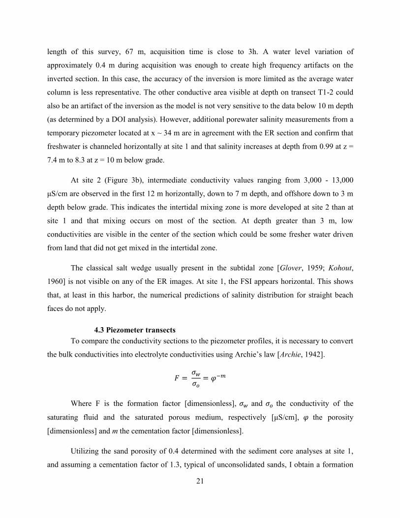
21

length of this survey, 67 m, acquisition time is close to 3h. A water level variation of

approximately 0.4 m during acquisition was enough to create high frequency artifacts on the

inverted section. In this case, the accuracy of the inversion is more limited as the average water

column is less representative. The other conductive area visible at depth on transect T1-2 could

also be an artifact of the inversion as the model is not very sensitive to the data below 10 m depth

(as determined by a DOI analysis). However, additional porewater salinity measurements from a

temporary piezometer located at x ~ 34 m are in agreement with the ER section and confirm that

freshwater is channeled horizontally at site 1 and that salinity increases at depth from 0.99 at z =

7.4 m to 8.3 at z = 10 m below grade.

At site 2 (Figure 3b), intermediate conductivity values ranging from 3,000 - 13,000

μS/cm are observed in the first 12 m horizontally, down to 7 m depth, and offshore down to 3 m

depth below grade. This indicates the intertidal mixing zone is more developed at site 2 than at

site 1 and that mixing occurs on most of the section. At depth greater than 3 m, low

conductivities are visible in the center of the section which could be some fresher water driven

from land that did not get mixed in the intertidal zone.

The classical salt wedge usually present in the subtidal zone [Glover, 1959; Kohout,

1960] is not visible on any of the ER images. At site 1, the FSI appears horizontal. This shows

that, at least in this harbor, the numerical predictions of salinity distribution for straight beach

faces do not apply.

4.3 Piezometer transects

To compare the conductivity sections to the piezometer profiles, it is necessary to convert

the bulk conductivities into electrolyte conductivities using Archie’s law [Archie, 1942].

Where F is the formation factor [dimensionless], and the conductivity of the

saturating fluid and the saturated porous medium, respectively [μS/cm], the porosity

[dimensionless] and m the cementation factor [dimensionless].

Utilizing the sand porosity of 0.4 determined with the sediment core analyses at site 1,

and assuming a cementation factor of 1.3, typical of unconsolidated sands, I obtain a formation

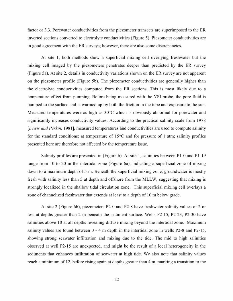
22

factor or 3.3. Porewater conductivities from the piezometer transects are superimposed to the ER

inverted sections converted to electrolyte conductivities (Figure 5). Piezometer conductivities are

in good agreement with the ER surveys; however, there are also some discrepancies.

At site 1, both methods show a superficial mixing cell overlying freshwater but the

mixing cell imaged by the piezometers penetrates deeper than predicted by the ER survey

(Figure 5a). At site 2, details in conductivity variations shown on the ER survey are not apparent

on the piezometer profile (Figure 5b). The piezometer conductivities are generally higher than

the electrolyte conductivities computed from the ER sections. This is most likely due to a

temperature effect from pumping. Before being measured with the YSI probe, the pore fluid is

pumped to the surface and is warmed up by both the friction in the tube and exposure to the sun.

Measured temperatures were as high as 30°C which is obviously abnormal for porewater and

significantly increases conductivity values. According to the practical salinity scale from 1978

[Lewis and Perkin, 1981], measured temperatures and conductivities are used to compute salinity

for the standard conditions: at temperature of 15°C and for pressure of 1 atm; salinity profiles

presented here are therefore not affected by the temperature issue.

Salinity profiles are presented in (Figure 6). At site 1, salinities between P1-0 and P1-19

range from 10 to 20 in the intertidal zone (Figure 6a), indicating a superficial zone of mixing

down to a maximum depth of 5 m. Beneath the superficial mixing zone, groundwater is mostly

fresh with salinity less than 5 at depth and offshore from the MLLW, suggesting that mixing is

strongly localized in the shallow tidal circulation zone. This superficial mixing cell overlays a

zone of channelized freshwater that extends at least to a depth of 10 m below grade.

At site 2 (Figure 6b), piezometers P2-0 and P2-8 have freshwater salinity values of 2 or

less at depths greater than 2 m beneath the sediment surface. Wells P2-15, P2-23, P2-30 have

salinities above 10 at all depths revealing diffuse mixing beyond the intertidal zone. Maximum

salinity values are found between 0 - 4 m depth in the intertidal zone in wells P2-8 and P2-15,

showing strong seawater infiltration and mixing due to the tide. The mid to high salinities

observed at well P2-15 are unexpected, and might be the result of a local heterogeneity in the

sediments that enhances infiltration of seawater at high tide. We also note that salinity values

reach a minimum of 12, before rising again at depths greater than 4 m, marking a transition to the

23

deep saline zone at site 2. The differences in porewater salinity distribution revealed by the ER

surveys are confirmed by the piezometer profiles.

4.4 Seepage measurements

4.4.1 Ultrasonic seepage meters

At site 1, the specific discharge measured at the end of May 2011, by funnel F1 is very

low, with an average of 3.6 cm/d (Figure 7a). The flow rate exhibits two high peaks at the

beginning of the recording period that do not match any precipitation event and may be artifacts

triggered by the disturbance of the mud layer during installation. Higher rates averaging 10 cm/d

are visible on day 3, as a consequence of the 0.51 cm precipitation falling that day. A Fourier

transform analysis confirmed the visible absence of correlation between SGD and tidal stage.

At site 2, seepage rates measured in May by funnel F2 are very high, with an average of

61.3 cm/d (Figure 7b). Seepage rates vary from -83.3 to 274.9 cm/d, with the latter magnitude

close to the highest values measured on Long Island [Paulsen et al., 2004] and other locations

throughout the world [Russoniello et al., 2013; Stieglitz et al., 2008a; Taniguchi et al., 2002].

The relationship between tidal stage and SGD is not consistent over time: from 5/19 to 5/21 high

tide coincides with a peak in SGD and from 5/21 to 5/25 high tide coincides with a local

minimum in an overall SGD peak. This is highly unusual and does not fit the general case where

a negative correlation is observed between the tides and SGD [Paulsen et al., 2004; Taniguchi

and Iwakawa, 2004; Taniguchi et al., 2006]. Both tidal and seepage signals have a period of

12.42 hours corresponding to the principal lunar semi-diurnal M2, and a period of 6.21 hours

corresponding to shallow water over tide of the principal lunar M4, as revealed by a Fourier

transform analysis. The seepage measurement period also coincides with a transition from spring

tide to neap tide, which adds another trend to the resulting tidal signal. The complexity of the

tidal signal could explain the complexity of SGD recorded at this site.

Funnels F3 and F4 exhibit relatively high average seepage rates: 109.3 cm/d and 29.8

cm/d, respectively. The approximation of an exponential decay of SGD with respect to distance

from shore does not apply at this site [Bokuniewicz, 1980; Mc Bride and Pfannkuch, 1975]. Both

funnels were placed approximately 40 m offshore of the MLLW, and did not reside within the

intertidal zone. SGD in F3 shows strong variations but they do not seem to be related to the tide.

SGD in F4 does not vary much and does not exhibit any correlation with the tide either. A

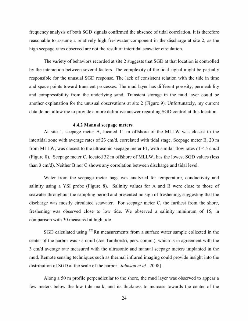
24

frequency analysis of both SGD signals confirmed the absence of tidal correlation. It is therefore

reasonable to assume a relatively high freshwater component in the discharge at site 2, as the

high seepage rates observed are not the result of intertidal seawater circulation.

The variety of behaviors recorded at site 2 suggests that SGD at that location is controlled

by the interaction between several factors. The complexity of the tidal signal might be partially

responsible for the unusual SGD response. The lack of consistent relation with the tide in time

and space points toward transient processes. The mud layer has different porosity, permeability

and compressibility from the underlying sand. Transient storage in the mud layer could be

another explanation for the unusual observations at site 2 (Figure 9). Unfortunately, my current

data do not allow me to provide a more definitive answer regarding SGD control at this location.

4.4.2 Manual seepage meters

At site 1, seepage meter A, located 11 m offshore of the MLLW was closest to the

intertidal zone with average rates of 23 cm/d, correlated with tidal stage. Seepage meter B, 20 m

from MLLW, was closest to the ultrasonic seepage meter F1, with similar flow rates of < 5 cm/d

(Figure 8). Seepage meter C, located 32 m offshore of MLLW, has the lowest SGD values (less

than 3 cm/d). Neither B nor C shows any correlation between discharge and tidal level.

Water from the seepage meter bags was analyzed for temperature, conductivity and

salinity using a YSI probe (Figure 8). Salinity values for A and B were close to those of

seawater throughout the sampling period and presented no sign of freshening, suggesting that the

discharge was mostly circulated seawater. For seepage meter C, the furthest from the shore,

freshening was observed close to low tide. We observed a salinity minimum of 15, in

comparison with 30 measured at high tide.

SGD calculated using 222

Rn measurements from a surface water sample collected in the

center of the harbor was ~5 cm/d (Joe Tamborski, pers. comm.), which is in agreement with the

3 cm/d average rate measured with the ultrasonic and manual seepage meters implanted in the

mud. Remote sensing techniques such as thermal infrared imaging could provide insight into the

distribution of SGD at the scale of the harbor [Johnson et al., 2008].

Along a 50 m profile perpendicular to the shore, the mud layer was observed to appear a

few meters below the low tide mark, and its thickness to increase towards the center of the

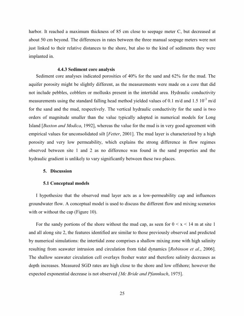
25

harbor. It reached a maximum thickness of 85 cm close to seepage meter C, but decreased at

about 50 cm beyond. The differences in rates between the three manual seepage meters were not

just linked to their relative distances to the shore, but also to the kind of sediments they were

implanted in.

4.4.3 Sediment core analysis

Sediment core analyses indicated porosities of 40% for the sand and 62% for the mud. The

aquifer porosity might be slightly different, as the measurements were made on a core that did

not include pebbles, cobblers or mollusks present in the intertidal area. Hydraulic conductivity

measurements using the standard falling head method yielded values of 0.1 m/d and 1.5 10-3

m/d

for the sand and the mud, respectively. The vertical hydraulic conductivity for the sand is two

orders of magnitude smaller than the value typically adopted in numerical models for Long

Island [Buxton and Modica, 1992], whereas the value for the mud is in very good agreement with

empirical values for unconsolidated silt [Fetter, 2001]. The mud layer is characterized by a high

porosity and very low permeability, which explains the strong difference in flow regimes

observed between site 1 and 2 as no difference was found in the sand properties and the

hydraulic gradient is unlikely to vary significantly between these two places.

5. Discussion

5.1 Conceptual models

I hypothesize that the observed mud layer acts as a low-permeability cap and influences

groundwater flow. A conceptual model is used to discuss the different flow and mixing scenarios

with or without the cap (Figure 10).

For the sandy portions of the shore without the mud cap, as seen for 0 < x < 14 m at site 1

and all along site 2, the features identified are similar to those previously observed and predicted

by numerical simulations: the intertidal zone comprises a shallow mixing zone with high salinity

resulting from seawater intrusion and circulation from tidal dynamics [Robinson et al., 2006].

The shallow seawater circulation cell overlays fresher water and therefore salinity decreases as

depth increases. Measured SGD rates are high close to the shore and low offshore; however the

expected exponential decrease is not observed [Mc Bride and Pfannkuch, 1975].

26

When the mud cap is present (Figure9b), as seen at site 1 for x > 14 m offshore of the

MLLW, groundwater is hydraulically isolated from the overlying seawater, which prevents

mixing and strongly limits SGD rates. Freshwater from land is channeled and directed offshore

as a result of the low permeability mud cap. SGD rates through the cap are very small and do not

seem to be correlated with the tides. The mud layer is not observed in the intertidal zone, and

therefore, a superficial mixing cell can develop [Robinson et al., 2006]. The influence of the cap

can also explain the relatively high seepage rates measured at site 2, relatively far from the shore.

The cap confines SGD to a large area by reducing vertical fluxes; hydraulic potential builds and

porewater flows horizontally to greater distances than expected. This agrees with mathematical

models of seepage in lake beds tested for different localization of low permeability bottom

sediments [Mc Bride and Pfannkuch, 1975] as well as direct field observations [Hirsch and

Randazzo, 2000]. A similar effect was observed by Bokuniewicz [1980], in Great South Bay on

Long Island, where his seepage meter measurements indicated the presence of a superficial clay

layer that significantly decreased SGD and funneled discharge further offshore. Michael et al.

[2005] observed an organic-rich muck layer that influenced vertical hydraulic gradients in

Waquoit Bay, MA. Discontinuities in the mud layer can explain the very high flow rates

observed offshore at site 2 and the variability of seepage rates at similar distances from the shore.

[Russoniello et al., 2013] also observed a fresh water plume beneath low permeability areas in an

estuarine setting where paleovalleys were filled in by mud and peat deposits.

5.2 Stony Brook Harbor SGD

Seepage rates measured in Stony Brook Harbor are similar to other values reported in the

literature, but the range in rates measured at the same distance from the shore is unprecedented.

Low rates of 3 cm/d measured in the mud cap are close to those measured by Bokuniewicz

[1980] in Great South Bay, where sediments are composed of a mix of sand and clay. Higher

rates of 26 cm/d measured in the intertidal zone are close to those reported at Osaka Bay, Japan

[Taniguchi et al., 2002] where seepage meters were implanted in muddy sands. The very high

rates measured at site 2 are close to the 73.7-105.2 cm/d reported in Barbados, West Indies in a

sandy environment [Lewis, 1987]. Our range of values is similar to the wide range observed in

Shelter Island, NY where sediments are composed of mostly sand, gravel and silt with seepage

rates varying from 14 cm/d to 225cm/d depending on the tidal level [Paulsen et al., 2004].

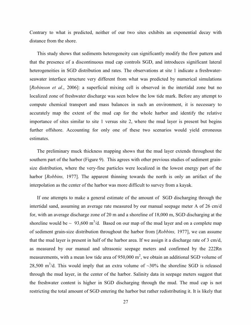
27

Contrary to what is predicted, neither of our two sites exhibits an exponential decay with

distance from the shore.

This study shows that sediments heterogeneity can significantly modify the flow pattern and

that the presence of a discontinuous mud cap controls SGD, and introduces significant lateral

heterogeneities in SGD distribution and rates. The observations at site 1 indicate a freshwater-

seawater interface structure very different from what was predicted by numerical simulations

[Robinson et al., 2006]: a superficial mixing cell is observed in the intertidal zone but no

localized zone of freshwater discharge was seen below the low tide mark. Before any attempt to

compute chemical transport and mass balances in such an environment, it is necessary to

accurately map the extent of the mud cap for the whole harbor and identify the relative

importance of sites similar to site 1 versus site 2, where the mud layer is present but begins

further offshore. Accounting for only one of these two scenarios would yield erroneous

estimates.

The preliminary muck thickness mapping shows that the mud layer extends throughout the

southern part of the harbor (Figure 9). This agrees with other previous studies of sediment grain-

size distribution, where the very-fine particles were localized in the lowest energy part of the

harbor [Robbins, 1977]. The apparent thinning towards the north is only an artifact of the

interpolation as the center of the harbor was more difficult to survey from a kayak.

If one attempts to make a general estimate of the amount of SGD discharging through the

intertidal sand, assuming an average rate measured by our manual seepage meter A of 26 cm/d

for, with an average discharge zone of 20 m and a shoreline of 18,000 m, SGD discharging at the

shoreline would be ~ 93,600 m3/d. Based on our map of the mud layer and on a complete map

of sediment grain-size distribution throughout the harbor from [Robbins, 1977], we can assume

that the mud layer is present in half of the harbor area. If we assign it a discharge rate of 3 cm/d,

as measured by our manual and ultrasonic seepage meters and confirmed by the 222Rn

measurements, with a mean low tide area of 950,000 m2, we obtain an additional SGD volume of

28,500 m3/d. This would imply that an extra volume of ~30% the shoreline SGD is released

through the mud layer, in the center of the harbor. Salinity data in seepage meters suggest that

the freshwater content is higher in SGD discharging through the mud. The mud cap is not

restricting the total amount of SGD entering the harbor but rather redistributing it. It is likely that

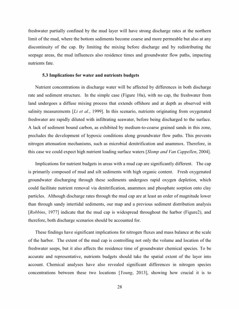
28

freshwater partially confined by the mud layer will have strong discharge rates at the northern

limit of the mud, where the bottom sediments become coarse and more permeable but also at any

discontinuity of the cap. By limiting the mixing before discharge and by redistributing the

seepage areas, the mud influences also residence times and groundwater flow paths, impacting

nutrients fate.

5.3 Implications for water and nutrients budgets

Nutrient concentrations in discharge water will be affected by differences in both discharge

rate and sediment structure. In the simple case (Figure 10a), with no cap, the freshwater from

land undergoes a diffuse mixing process that extends offshore and at depth as observed with

salinity measurements [Li et al., 1999]. In this scenario, nutrients originating from oxygenated

freshwater are rapidly diluted with infiltrating seawater, before being discharged to the surface.

A lack of sediment bound carbon, as exhibited by medium-to-coarse grained sands in this zone,

precludes the development of hypoxic conditions along groundwater flow paths. This prevents

nitrogen attenuation mechanisms, such as microbial denitrification and anammox. Therefore, in

this case we could expect high nutrient loading surface waters [Slomp and Van Cappellen, 2004].

Implications for nutrient budgets in areas with a mud cap are significantly different. The cap

is primarily composed of mud and silt sediments with high organic content. Fresh oxygenated

groundwater discharging through these sediments undergoes rapid oxygen depletion, which

could facilitate nutrient removal via denitrification, anammox and phosphate sorption onto clay

particles. Although discharge rates through the mud cap are at least an order of magnitude lower

than through sandy intertidal sediments, our map and a previous sediment distribution analysis

[Robbins, 1977] indicate that the mud cap is widespread throughout the harbor (Figure2), and

therefore, both discharge scenarios should be accounted for.

These findings have significant implications for nitrogen fluxes and mass balance at the scale

of the harbor. The extent of the mud cap is controlling not only the volume and location of the

freshwater seeps, but it also affects the residence time of groundwater chemical species. To be

accurate and representative, nutrients budgets should take the spatial extent of the layer into

account. Chemical analyses have also revealed significant differences in nitrogen species

concentrations between these two locations [Young, 2013], showing how crucial it is to

29

understand the hydrogeological framework before studying chemical reactions and species

distribution.

5.4 Sources of error

The Trident probe can be a useful tool to identify zones of fresh SGD. The portability of the

probe and the short time span required for the measurements allows one to cover a large area in a

relatively small amount of time. During this study, dissolved gas measurements needed to be

performed as soon as possible after the end of the winter [Young, 2013] which constrained the

timeframe for the Trident screening. Using the Trident at the winter/spring transition limited the

use of temperature signal as a fresh SGD indicator as strong temperature variations on a few days

was enough to create artifacts on the temperature signal. This might have prevented

identification of other strong fresh SGD areas. In the future, it will be best to use the Trident

probe away from seasonal transitions to ensure a temporal consistency in temperature

measurements.

ER surveys can be a helpful tool to image fluid distribution in the ground as fluid

conductivities can vary up to 6 orders of magnitude in coastal settings. However, ER

performances can be limited by various factors that must be taken into account prior to any

interpretation. In general, the sensitivity of the model decreases with depth and therefore, the

DOI must be assessed for each specific setting. For our double-cable ER survey we found that

the long time period required for acquisition was problematic, as the tides caused the water

column thickness to vary by 0.4 m during data collection, enough to produce noise and create

artifacts during the inversion. The beach topography and the broad tidal range in Stony Brook

Harbor limited the use of long ER surveys. Surveys planning and forward modeling can help

design better suited surveys for a particular setting, but the EI2D is limited by its forward

modeling options, as it does not allow to include topography and underwater electrodes.

Direct pore-water analysis can be an appropriate way to constrain an inversion or check the

ER results [Henderson et al., 2010]. The piezometer transects provided in situ salinity

measurements that enabled us to distinguish between areas with different salt content and

compare them to the ER sections. Unfortunately, the comparison was limited by the time

discrepancies between acquisition campaigns for each method and precipitation events occurring

30

during piezometer data collection. The ER surveys represented snapshots, over 45 minutes, of

the fluid distribution at high tide, whereas the piezometer transects were done point by point

during 8 consecutive days each, at various tidal levels.

As described in details by Young [2013], a cluster monitoring well was installed in the

intertidal zone, between piezometers P1-7 and P1-19 (Figure 1b). Individual wells were

screened at a constant interval of 0.9 m (3’), screen length was 0.15 m. Ten sampling depths

varied between 0.91 to 9.1 meters below grade, with a 0.9 m interval. Samples were collected

daily between 9:30 am to 10:30am EST, 27 day period between 9/26/11 and 10/25/11. The

analysis of the sample shows that salinities are consistent over time at a given depth [Young,

2013]: the salinity structure appears stable over two spring-neap tidal cycles, which allows us to

compare our resistivity and piezometer profiles in spite of the time discrepancies in acquisition.

The direct conductivity comparison was hindered by a temperature effect resulting from the

pumping and exposure to the surface before measurements. This could be prevented by having

C/T probes directly into the piezometers which was not possible for this study.

Due to the diffuse nature of SGD, seepage meter measurements can vary significantly at

various scales [Michael et al., 2003; Michael et al., 2005; Rosenberry, 2008; Russoniello et al.,

2013; Shaw and Prepas, 1989]. Concurrent measurements are therefore necessary to ensure the

validity of the measurements. Due to technical difficulties, I was unable to obtain a grid of

seepage data but isotopes derived fluxes provided estimates that were in agreement with our

seepage data (Joe Tamborski, pers. comm.). The slightly higher rate measured above the mud

can be the result of the spatial integration of Rn measurements or due to SGD annual variations

during the two-year time span between seepage and Rn measurements.

Manual and ultrasonic seepage meters were also in very good agreement. In high energy

settings, flow can be enhanced around the seepage meters due to hydrodynamic interactions

[Shaw and Prepas, 1989; Shinn et al., 2002], but fluxes were sufficiently high to ignore these

and our sites were wave and current free thus limiting the Bernoulli effect [Cable et al., 2006;

Corbett and Cable, 2003]. During installation of the manual seepage meters, there is always

some surface water that is trapped into the sediments and interpreting the salinity in the seepage

bags as that of SGD would be erroneous. Seepage rates as low as measured in the manual

seepage C (< 3cm/d) were insufficient to entirely flush the seepage meter during the period of

31

observation. However, the significant freshening observed confirms the presence of fresh water

far into the subtidal zone and supports the hypothesis that freshwater is channeled from land

towards the center of the harbor by the low permeability mud layer.

6. Conclusion

Our integrated approach using a direct-push probe, electrical resistivity surveys, piezometer

transects and seepage meter measurements was successful in identifying the complexity of SGD

characteristics at large and small scales in Stony Brook Harbor. The comparison between the

results of different methods revealed remarkable agreement. Piezometer transects validated the

reliability of electrical resistivity surveys in a challenging environment such as tidally dominated

harbors.

This study emphasizes that the distribution of SGD in embayments differs from numerical

predictions for straight beach faces when low-permeability bottom sediments are present. The

deposition of fine particle mud layers is likely to happen in many places where there is a

significant loss of energy from the ocean. SGD can be distributed throughout the whole harbor

and not just close to the shore, as models predict. A superficial low permeability mud layer can

control groundwater flow and affect pathways and residence times which will have implications

both on water budgets and on chemical reactions and therefore nutrients budgets. The channeling

of freshwater offshore as a result of the mud layer could also be enhanced by the curvature of the

shore that would focus groundwater towards the center of the harbor. More investigations on the

effect of low permeability mud layers and shoreline curvature are necessary, as well as the study

of their joint effect on SGD. Numerical modeling more specific to bay environments would be

very beneficial to determine what characteristics a mud layer would impact groundwater flow,

and to make these results more applicable to other settings. We recommend investigating the

presence of such layer in similar low-energy coastal environments prior to any SGD study and

characterizing its extent and properties before attempting any regional SGD estimates.

Acknowledgments

The study at Stony Brook University was partially funded by the NY Seagrant Research

Program, through the grant –R/CTP-44-NYCT. We are grateful to the Office of Water Resources

of Suffolk County Health Department for providing technical assistance in the field, including

32

the installation of monitoring wells within the study area. The data acquisition would not have

been possible without the significant contributions of F. Basile, M. Buzby, E. Ericksen, R.

Milito, R. Paulsen, N. Stark, L. Velasquez, M. Velasquez and J. Wanlass.

33

References

AGI (2009), Instruction Manual for EarthImager 2D, Version 2.4.0, Resistivity and IP

Iversion Software, Austin, Texas, Report.

Anderson, M. P. (2005), Heat as a ground water tracer, Groundwater, 43(6), 951-968.

Archie, G. (1942), The electrical resistivity log as an aid in determining some reservoir

characteristics, Trans. AIME, 146(99), 54-62.

Befus, K. M., M. B. Cardenas, D. V. Erler, I. R. Santos, and B. D. Eyre (2013), Heat

transport dynamics at a sandy intertidal zone, Water Resources Research, 49(6), 3770-3786.



Bokuniewicz, H., M. Taniguchi, T. Ishitoibi, M. Charette, M. Allen, and E. A. Kontar (2008),

Direct measurements of submarine groundwater discharge (SGD) over a fractured rock aquifer in

Flamengo Bay Brazil, Estuarine Coastal and Shelf Science, 76(3), 466-472.



Bratton, J. F., S. M. Colman, E. R. Thieler, and R. R. Seal (2002), Birth of the modern

Chesapeake Bay estuary between 7.4 and 8.2 ka and implications for global sea-level rise, Geo-

Marine Letters, 22(4), 188-197.

Bratton, J. F., J. K. Böhlke, F. T. Manheim, and D. E. Krantz (2004), Ground Water Beneath

Coastal Bays of the Delmarva Peninsula: Ages and Nutrients, Ground Water, 42(7), 1021-1034.

Bratton, J. F., W. Sanford, C. Langevin, M. Polemio, and P. Povinec (2007), The importance

of shallow confining units to submarine groundwater flow, paper presented at Proceedings of the

Symposium" A New Focus on Groundwater-Seawater Interactions" at the 24th General

Assembly of the International Union of Geodesy and Geophysics, Perugia, Italy, 2-13 July 2007.,

IAHS Press.



Buxton, H. T., and E. Modica (1992), Patterns and rates of ground-water movement on Long

Island, New York, Ground Water, V. 30(No. 6), p. 857-866.

Cable, J. E., J. B. Martin, and J. Jaeger (2006), Exonerating Bernoulli? On evaluating the

physical and biological processes affecting marine seepage meter measurements, Limnology and

Oceanography: Methods, 4, 172-183.

Chadwick, D. B., A. Gordon, J. Groves, C. Smith, R. Paulsen, and B. Harre (2003), New

tools for monitoring coastal contaminant migration, Sea technology, 44(6), 17-22.

34




Charette, M. A., and M. C. Allen (2006), Precision Ground Water Sampling in Coastal

Aquifers Using a Direct‐Push, Shielded‐Screen Well‐Point System, Ground Water Monitoring &

Remediation, 26(2), 87-93.



Constable, S. C., R. L. Parker, and C. G. Constable (1987), Occam's inversion: A practical

algorithm for generating smooth models from electromagnetic sounding data, Geophysics, 52(3),

289-300.

Corbett, D. R., and J. E. Cable (2003), Seepage meters and advective transport in coastal

environments: Comments on “Seepage meters and Bernoulli's revenge” by EA Shinn, CD Reich,

and TD Hickey. 2002. Estuaries 25: 126–132, Estuaries and Coasts, 26(5), 1383-1387.

Cross, V., D. S. Foster, and J. F. Bratton (2010), Continuous resistivity profiling and

seismic-reflection data collected in 2006 from the Potomac River estuary, Virginia and

MarylandRep.

Day-Lewis, F., E. White, C. Johnson, J. Lane Jr, and M. Belaval (2006), Continuous

resistivity profiling to delineate submarine groundwater discharge--examples and limitations,

The Leading Edge, 25(6), 724.

Dimova, N. T., P. W. Swarzenski, H. Dulaiova, and C. R. Glenn (2012), Utilizing

multichannel electrical resistivity methods to examine the dynamics of the fresh water–seawater

interface in two Hawaiian groundwater systems, Journal of Geophysical Research, 117(C2),

C02012.

Fetter, C. (2001), Applied Hydrogeology (4 th), edited, New Jersey.

Gardner, L. R., and A. M. Wilson (2006), Comparison of four numerical models for

simulating seepage from salt marsh sediments, Estuarine, Coastal and Shelf Science, 69(3), 427-

437.

Gibbes, B., C. Robinson, L. Li, and D. Lockington (2007), Measurement of hydrodynamics

and pore water chemistry in intertidal groundwater systems, Journal of Coastal Research, SI, 50,

884-894.

Glover, R. (1959), The pattern of fresh-water flow in a coastal aquifer, Journal of

Geophysical Research, 64(4), 457-459.

Gross, M. G. (1972), Characteristics and environmental quality of six north shore bays:

Nassau and Suffolk Counties, Long Island, New YorkRep. 14, Stony Brook, New York: Marine

Science Research Center, State University of New York.

35

Henderson, R. D., F. D. Day-Lewis, E. Abarca, C. F. Harvey, H. N. Karam, L. B. Liu, and J.

W. Lane (2010), Marine electrical resistivity imaging of submarine groundwater discharge:

sensitivity analysis and application in Waquoit Bay, Massachusetts, USA, Hydrogeology Journal,

18(1), 173-185.

Hirsch, J., and A. Randazzo (2000), Hydraulic seepage within an astatic karst lake, North-

Central Florida'.



75-139.










Kroeger, K., and M. Charette (2008), Nitrogen biogeochemistry of submarine groundwater

discharge, Limnology and Oceanography, 53(3), 1025-1039.

Kuan, W. K., G. Jin, P. Xin, C. Robinson, B. Gibbes, and L. Li (2012), Tidal influence on

seawater intrusion in unconfined coastal aquifers, Water Resources Research, 48(2), W02502.



Lewis, E., and R. Perkin (1981), The practical salinity scale 1978: Conversion of existing

data, Deep Sea Research Part A. Oceanographic Research Papers, 28(4), 307-328.

Lewis, J. B. (1987), Measurements of groundwater seepage flux onto a coral reef: Spatial

and temporal variations, Limnology and Oceanography, 32(5), 1165-1169.



Manheim, F. T., D. E. Krantz, and J. F. Bratton (2004), Studying ground water under

Delmarva coastal bays using electrical resistivity, Groundwater, 42(7), 1052-1068.

Marshall, T. J., J. W. Holmes, and C. W. Rose (1996), Soil physics, Cambridge University

Press.

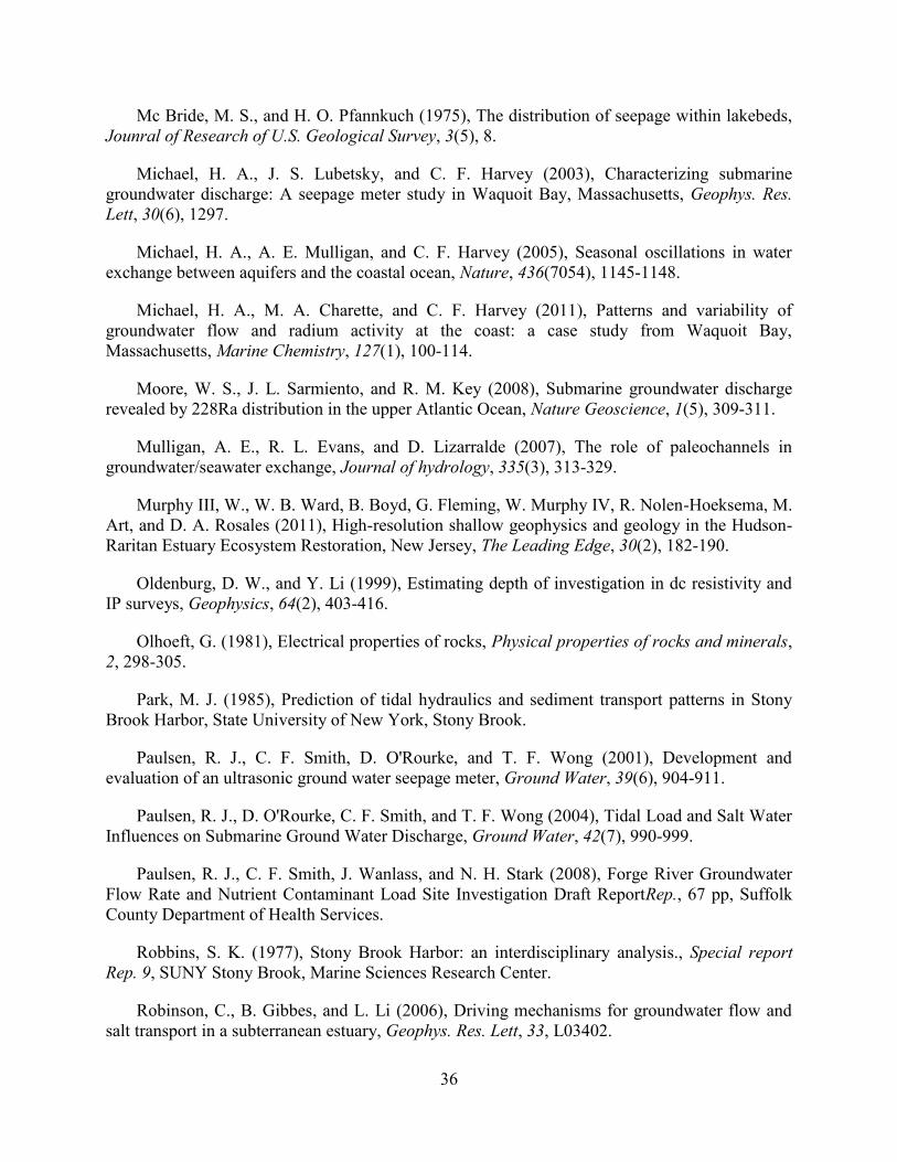
36

Mc Bride, M. S., and H. O. Pfannkuch (1975), The distribution of seepage within lakebeds,

Jounral of Research of U.S. Geological Survey, 3(5), 8.



Lett, 30(6), 1297.



Michael, H. A., M. A. Charette, and C. F. Harvey (2011), Patterns and variability of

groundwater flow and radium activity at the coast: a case study from Waquoit Bay,

Massachusetts, Marine Chemistry, 127(1), 100-114.



Mulligan, A. E., R. L. Evans, and D. Lizarralde (2007), The role of paleochannels in

groundwater/seawater exchange, Journal of hydrology, 335(3), 313-329.

Murphy III, W., W. B. Ward, B. Boyd, G. Fleming, W. Murphy IV, R. Nolen-Hoeksema, M.

Art, and D. A. Rosales (2011), High-resolution shallow geophysics and geology in the Hudson-

Raritan Estuary Ecosystem Restoration, New Jersey, The Leading Edge, 30(2), 182-190.

Oldenburg, D. W., and Y. Li (1999), Estimating depth of investigation in dc resistivity and

IP surveys, Geophysics, 64(2), 403-416.

Olhoeft, G. (1981), Electrical properties of rocks, Physical properties of rocks and minerals,

2, 298-305.

Park, M. J. (1985), Prediction of tidal hydraulics and sediment transport patterns in Stony

Brook Harbor, State University of New York, Stony Brook.





Paulsen, R. J., C. F. Smith, J. Wanlass, and N. H. Stark (2008), Forge River Groundwater

Flow Rate and Nutrient Contaminant Load Site Investigation Draft ReportRep., 67 pp, Suffolk

County Department of Health Services.

Robbins, S. K. (1977), Stony Brook Harbor: an interdisciplinary analysis., Special report

Rep. 9, SUNY Stony Brook, Marine Sciences Research Center.



37

Rosenberry, D. O. (2008), A seepage meter designed for use in flowing water, Journal of

Hydrology, 359(1), 118-130.

Russoniello, C. J., C. Fernandez, J. F. Bratton, J. F. Banaszak, D. E. Krantz, A. S. Andres, L.

F. Konikow, and H. A. Michael (2013), Geologic effects on groundwater salinity and discharge

into an estuary, Journal of Hydrology, 498, 1-12.

Shaw, R., and E. Prepas (1989), Anomalous, short-term influx of water into seepage meters,

Limnology and Oceanography, 34(7), 1343-1351.

Shinn, E. A., C. D. Reich, and T. D. Hickey (2002), Seepage meters and Bernoulli’s revenge,

Estuaries, 25(1), 126-132.



64-86.

Stieglitz, T., M. Taniguchi, and S. Neylon (2008a), Spatial variability of submarine

groundwater discharge, Ubatuba, Brazil, Estuarine Coastal and Shelf Science, 76(3), 493-500.






543-550.

Swarzenski, P. W., F. W. Simonds, A. J. Paulson, S. Kruse, and C. Reich (2007),

Geochemical and geophysical examination of submarine groundwater discharge and associated

nutrient loading estimates into Lynch Cove, Hood Canal, WA, Environmental Science &

Technology, 41(20), 7022-7029.

Swarzenski, P. W., W. C. Burnett, W. J. Greenwood, B. Herut, R. Peterson, N. Dimova, Y.

Shalem, Y. Yechieli, and Y. Weinstein (2006), Combined time-series resistivity and geochemical

tracer techniques to examine submarine groundwater discharge at Dor Beach, Israel,




Taniguchi, M., and H. Iwakawa (2004), Submarine groundwater discharge in Osaka Bay,

Japan, Limnology, 5(1), 25-32.



38

Taniguchi, M., T. Ishitobi, W. C. Burnett, and G. Wattayakorn (2007), Evaluating ground

water–sea water interactions via resistivity and seepage meters, Ground Water, 45(6), 729-735.




Taylor, R. W., and D. S. Cherkauer (1984), The application of combined seismic and

electrical measurements to the determination of the hydraulic conductivity of a lake bed,

Groundwater Monitoring & Remediation, 4(4), 78-85.

Telford, W. M., L. Geldart, and R. E. Sheriff (1990), Applied geophysics, Cambridge Univ

Pr.






Coasts, 15(4), 443-457.

Weinstein, Y., W. C. Burnett, P. W. Swarzenski, Y. Shalem, Y. Yechieli, and B. Herut

(2007), Role of aquifer heterogeneity in fresh groundwater discharge and seawater recycling: An

example from the Carmel coast, Israel, Journal of Geophysical Research-Oceans, 112(C12).

Wilson, A. M., and L. R. Gardner (2006), Tidally driven groundwater flow and solute

exchange in a marsh: numerical simulations, Water Resources Research, 42(1).



http://www.geo.sunysb.edu/reports/cyoung-phd-thesis.pdf


Press Inc.

39

Figures and captions

Figure 1. (a) Site map of Stony Brook Harbor and inclusion of general location. (b) Cross

section of relative positions of the different measurements at site 1. (c) Cross section of relative

positions of the different measurements at site 2. The vertical black dotted lines indicate the

piezometer wells. The number following the P indicates the site and the number after the hyphen,

the distance from the first piezometer. The grey dots show the positions of the manual seepage

meters. The stars, F, indicate the positions of the ultrasonic seepage meter funnels. The electrical

resistivity transects, T, are plotted as solid or dotted lines with black inverted triangles. The black

cross (x) indicate the position of the mean lower level of water (MLLW). The high tide mark

would be landward of the first piezometer at each site. The sections are presented with 5x

vertical exaggeration.

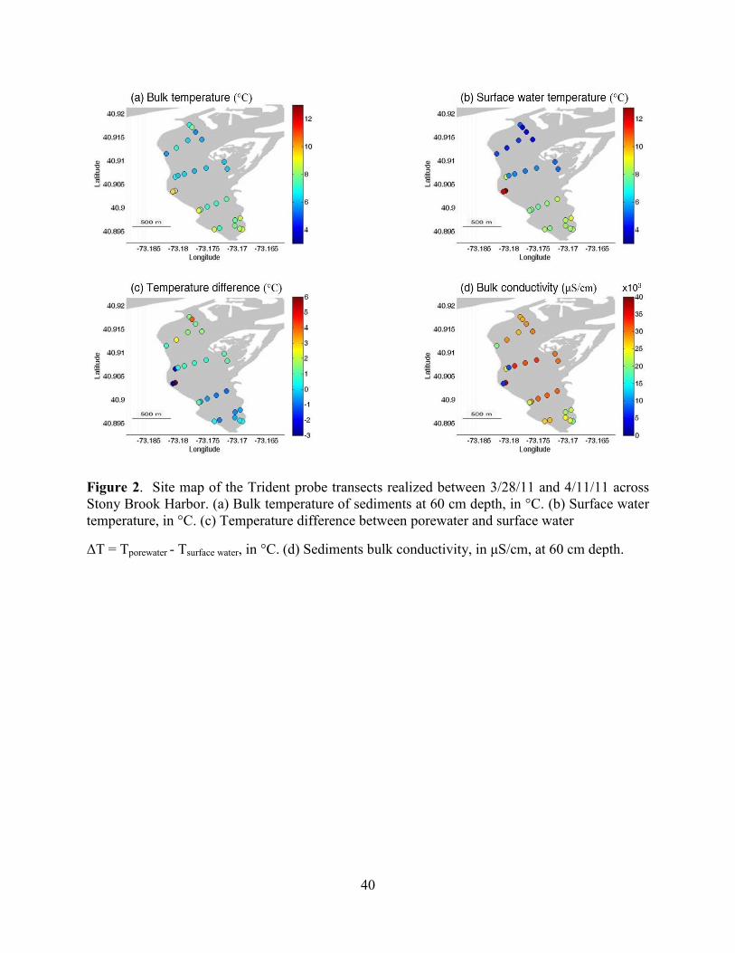
40

Figure 2. Site map of the Trident probe transects realized between 3/28/11 and 4/11/11 across

Stony Brook Harbor. (a) Bulk temperature of sediments at 60 cm depth, in °C. (b) Surface water

temperature, in °C. (c) Temperature difference between porewater and surface water

ΔT = Tporewater - Tsurface water, in °C. (d) Sediments bulk conductivity, in μS/cm, at 60 cm depth.

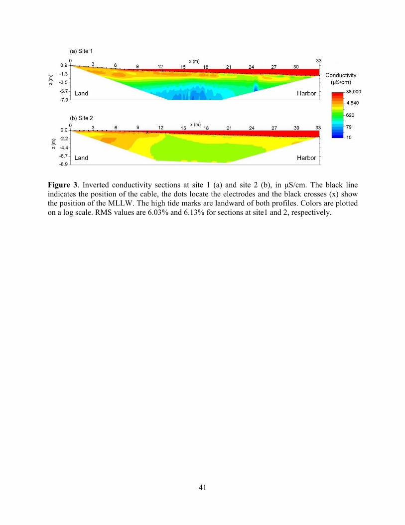
41

Figure 3. Inverted conductivity sections at site 1 (a) and site 2 (b), in μS/cm. The black line

indicates the position of the cable, the dots locate the electrodes and the black crosses (x) show

the position of the MLLW. The high tide marks are landward of both profiles. Colors are plotted

on a log scale. RMS values are 6.03% and 6.13% for sections at site1 and 2, respectively.

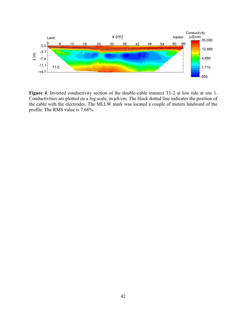
42

Figure 4. Inverted conductivity section of the double-cable transect T1-2 at low tide at site 1.

Conductivities are plotted on a log scale, in μS/cm. The black dotted line indicates the position of

the cable with the electrodes. The MLLW mark was located a couple of meters landward of the

profile. The RMS value is 7.68%.

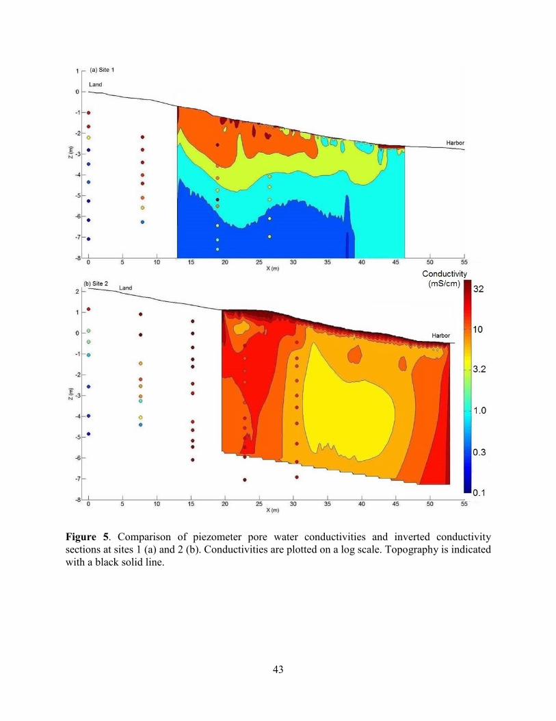
43

Figure 5. Comparison of piezometer pore water conductivities and inverted conductivity

sections at sites 1 (a) and 2 (b). Conductivities are plotted on a log scale. Topography is indicated

with a black solid line.

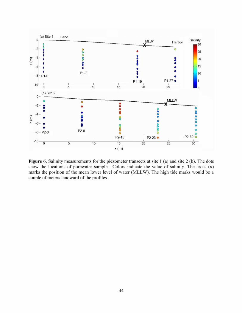
44

Figure 6. Salinity measurements for the piezometer transects at site 1 (a) and site 2 (b). The dots

show the locations of porewater samples. Colors indicate the value of salinity. The cross (x)

marks the position of the mean lower level of water (MLLW). The high tide marks would be a

couple of meters landward of the profiles.

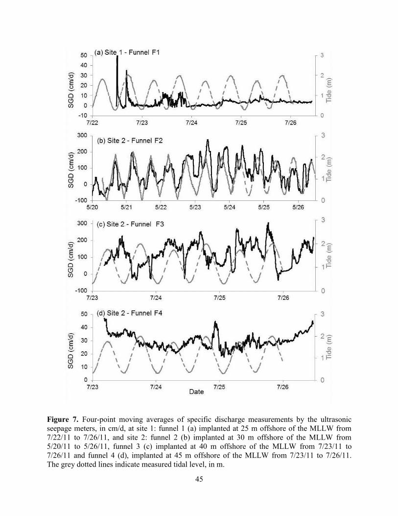
45

Figure 7. Four-point moving averages of specific discharge measurements by the ultrasonic

seepage meters, in cm/d, at site 1: funnel 1 (a) implanted at 25 m offshore of the MLLW from

7/22/11 to 7/26/11, and site 2: funnel 2 (b) implanted at 30 m offshore of the MLLW from

5/20/11 to 5/26/11, funnel 3 (c) implanted at 40 m offshore of the MLLW from 7/23/11 to

7/26/11 and funnel 4 (d), implanted at 45 m offshore of the MLLW from 7/23/11 to 7/26/11.

The grey dotted lines indicate measured tidal level, in m.

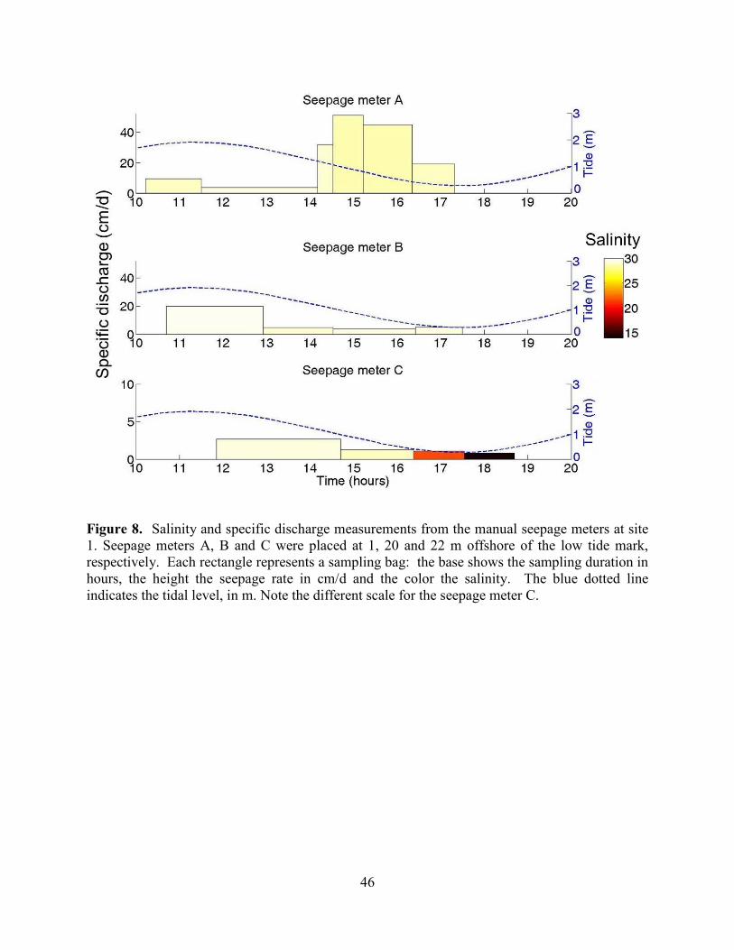
46

Figure 8. Salinity and specific discharge measurements from the manual seepage meters at site

1. Seepage meters A, B and C were placed at 1, 20 and 22 m offshore of the low tide mark,

respectively. Each rectangle represents a sampling bag: the base shows the sampling duration in

hours, the height the seepage rate in cm/d and the color the salinity. The blue dotted line

indicates the tidal level, in m. Note the different scale for the seepage meter C.

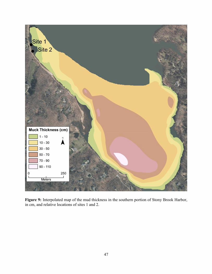
47

Figure 9: Interpolated map of the mud thickness in the southern portion of Stony Brook Harbor,

in cm, and relative locations of sites 1 and 2.

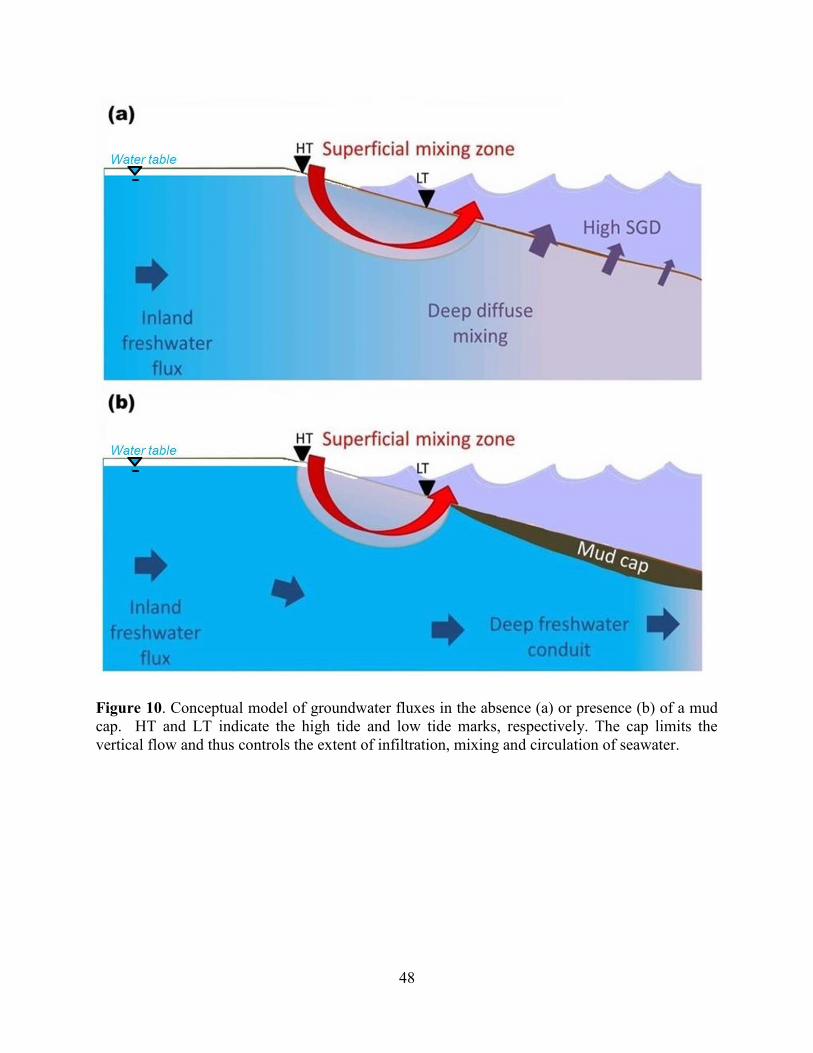
48

Figure 10. Conceptual model of groundwater fluxes in the absence (a) or presence (b) of a mud

cap. HT and LT indicate the high tide and low tide marks, respectively. The cap limits the

vertical flow and thus controls the extent of infiltration, mixing and circulation of seawater.

49

Chapter 3: Groundwater flow and solute transport modeling of a coastal unconfined sandy

aquifer: application to Stony Brook Harbor

Abstract

A field study of spatial distribution of submarine groundwater discharge (SGD) in Stony

Brook Harbor, NY suggested that it is controlled by a low-permeability mud layer, spreading

throughout approximately a third of the harbor area. Published numerical models developed

for homogeneous, isotropic unconfined aquifers with tidal forcing are in discrepancy with

observations at Stony Brook Harbor. Active sedimentation of fine particle is common in low

energy environments; it is therefore of interest to investigate the role of such a layer using a

more specific model. Comparative 2D SEAWAT density-difference groundwater flow and

transport models were developed. Steady-state simulations with and without the mud layer

were able to reproduce field observations. A 50 cm thick layer with a hydraulic conductivity

of 0.01 m/d at the surface of the sediments is sufficient to significantly alter the hydraulic

gradient and salinity distribution under the mud.

50

1. Introduction

With about 44% of the current world population living within 150 km of the coasts, pressure

on coastal groundwater resources and seawater intrusion constitute major concerns that need to

be addressed [Bear, 1999]. Predicting the freshwater-seawater interface (FSI) position and

dynamics is therefore crucial. Empirically, the Ghyben-Herzberg relation states that the FSI

should be found at a depth equal to 40 times the hydraulic head on land, with sea level as

reference [Badon-Ghyben, 1888; Herzberg, 1901]. Hydrodynamic equilibrium predicts the

existence of a saltwater wedge limiting a density-driven convection cell model [Cooper Jr, 1959;

Glover, 1959; Kohout, 1960]. Recently, improved numerical models have allowed the inclusion

of dynamic boundary conditions, such as waves and tides, that lead to predictions of a more

complex FSI [Robinson et al., 2006; Robinson et al., 2007a; Robinson et al., 2007b; Robinson et

al., 2007c]. Current numerical models indicate that the FSI should have three main components:

a superficial mixing cell located in the intertidal zone, a freshwater discharge area close to the

low tide mark and the saltwater wedge. The size and position of these features are contingent

upon the relative importance of several factors: the inland hydraulic gradient, the slope of the

beach, the tidal and wave amplitude [Robinson et al., 2007b].

Submarine groundwater discharge (SGD) encompasses all fluids that cross the sediment

ocean interface, regardless of their origin or composition [Burnett et al., 2003]. This means that

SGD includes fresh water derived from inland hydraulic gradient, intrusion of seawater and any

discharge of circulated seawater, no matter what the driving force is. Studying SGD in coastal

settings is challenging due to the highly dynamic boundary conditions and variety of physical

drivers responsible for different SGD components. Numerical simulations have proved very

useful in isolating and studying the effects of individual variables, as well as various

combinations of factors. A stronger hydraulic gradient sharpens the FSI and pushes it offshore

[Prieto and Destouni, 2005; Robinson et al., 2007a]. Tides and waves influence the chemistry of

SGD by enhancing the circulated seawater fraction [Gibbes et al., 2008a; Gibbes et al., 2008b; Li

et al., 1999; Robinson et al., 2007a; Robinson et al., 2007b; Xin et al., 2010]. An inclined beach

slope intensifies seawater intrusion at high tidal levels [Ataie-Ashtiani et al., 1999; Mango et al.,

2004; Mao et al., 2006], while spring-neap tides and seasonal recharge cycles influence the

position of the FSI and the associated chemical loading on longer time scales [Michael et al.,

51

2005; Turner et al., 1997]. Interactions with the seabed topography can also enhance SGD

[Konikow et al., 2013]. Field and laboratory measurements coupled with numerical simulations

suggested that the pathways SGD takes through the different parts of the FSI may influence the

associated chemical reactions by affecting solute residence time [Beck et al., 2007a; Gibbes et

al., 2008a; Gibbes et al., 2008b; Kuan et al., 2012; Mulligan and Charette, 2006].

Realistic modeling of the hydrologic system would require not only the representation of

dynamic boundaries but also several other factors such as density variations, spatial variability

and diffusivity of phenomena [Burnett et al., 2006; Michael et al., 2003; Michael et al., 2005],

heterogeneities, processes in the unsaturated zone [Heiss et al., 2014] and scale dependent

processes [Bratton, 2010; Smith, 2004]. The interactions among these variables still need further

investigations. Most current numerical models are limited to isotropic, homogeneous aquifers

with straight beach faces. This idealized case might not be suitable for understanding regional

scale SGD, including harbors and bays. First, a concave shoreline is known to focus groundwater

flow [Cherkauer and McKereghan, 1991; Lewandowski et al., 2013; Winter and Pfannkuch,

1984]. The existence of fine-particle low-permeability layer was investigated using flow nets, but

it has only been modeled for lakes where there are no density-driven or changes in water level

due to tides and waves [Mc Bride and Pfannkuch, 1975]. Second, the loss of energy between the

ocean and an embayment can deposit layers of fine particles or mud, with porosity and

permeability that are significantly different from the ones of the coastal aquifer. Analytical

models investigating the influence of a low permeability layer in lakes concluded that discharge

is focused at the shore independently of the layer [Mc Bride and Pfannkuch, 1975], but our field

observations at Stony Brook Harbor suggest otherwise (see chapter 2). To study SGD at larger

scales, it is necessary to characterize SGD distribution in embayments, as they do represent a

significant portion of the shoreline. The first step, presented here, focuses on studying the

influence of a low-permeability mud layer on SGD distribution in Stony Brook Harbor, NY. To

my knowledge, this is the first attempt at developing a 2D density-difference groundwater flow

and transport model for a heterogeneous aquifer.

SEAWAT is a density-dependent code [Guo and Langevin, 2002] that allows the simulation

of freshwater-seawater interactions in coastal environments by coupling the functionalities of the

groundwater simulator MODFLOW [Harbaugh et al., 2000] and the solute transport code

52

MT3DMS [Zheng and Wang, 1999b]. It is used here to simulate SGD in an unconfined sandy

aquifer with a sloping beach. With this model, we show that SGD distribution is controlled by

the spatial extent of a mud layer. A layer as thin as 50 cm is enough to substantially change SGD

amplitude, composition and location by modifying the hydraulic gradient and restricting mixing

with seawater.

2. Mathematical model

Several assumptions are made while developing the governing equation of groundwater flow

and solute transport in SEAWAT. It is assumed that Darcy’s law is valid, which means that the

flow is laminar. The standard expression for specific storage in a confined aquifer is applicable.

Fick’s law of diffusion is valid and isothermal conditions prevail. Active cells are assumed to be

fully saturated with water and finally, a fully miscible liquid phase of very small compressibility

is assumed [Guo and Langevin, 2002; Langevin et al., 2003].

SEAWAT uses the concept of equivalent freshwater head. In a saline groundwater

environment, heads vary with pressure, elevation and density. To prevent increased complexity

of governing equations, all heads are converted to freshwater heads by applying a density-

dependent correction (Equation 1).

(Equation 1)

where is the head [L], is the equivalent freshwater head [L], is the density of saline

aquifer water [ML-3

], is the density of freshwater [ML-3

] and Z is the elevation above 0 [L].

The basis of the governing equation for ground-water flow is the conservation of mass for

fluid and solute (Equation 2):

( ) ( )

(Equation 2)

where is the fluid density [ML-3

], is the specific discharge vector [LT-1

], is the density of

water entering from a source or leaving through a sink [ML-3

], qs is the volumetric flow rate per

unit volume of aquifer representing sources and sinks [T-1

], ne is the effective porosity

[dimensionless], and t is time [T].

53

Using the chain rule, differentiating with respect to time and pressure, identifying the

compressibility factors for the porous medium and the fluid, the flow equation becomes

(Equation 3):

( )

(Equation 3)

where P is the pore fluid pressure [ML-1

T-2

], C is the solute concentration [ML-3

], and Sp is the

specific storage in terms of pressure [M-1

LT-2

]. Details of the calculations are available in the

SEAWAT user manual [Guo and Langevin, 2002].

The specific discharge used in the flow equation is calculated using Darcy’s law for each

direction, assuming that the axes are in alignment with the principal permeability directions and

expressing the heads in term of equivalent freshwater heads, yields the governing equation for

saturated density-dependent groundwater flow (Equation 4):

[ (

)]

(Equation 4)

where z is the vertical coordinate directing upward [L], Kf is the equivalent freshwater hydraulic

conductivity [LT-1

], hf is the equivalent freshwater head [L], ρ is the fluid density [ML-3

], ρf is the

freshwater fluid density [ML-3

], Sf is the equivalent freshwater storage coefficient [L-1

], t is time

[T], ne is the effective porosity, ρs and qs are the density and flow rate per unit volume of aquifer

of the sources and sinks, respectively.

In SEAWAT, transport is coupled to groundwater flow. The governing equation for salt

transport is (Equation 5):

( )

( ) ( ) (Equation 5)

where C is the concentration of dissolved salt [ML-3

], D is the hydrodynamic dispersion

coefficient tensor [L2T

-1], the pore water velocity [LT

-1], and Cs is the concentration of

dissolved salt from the sources/sinks [ML-3

] [Zheng and Wang, 1999a].

A state equation relates the fluid density to its salt concentration (Equation 6).

(Equation 6)

54

where

is known to be approximately 0.7143 with C and ρ expressed in kg/m

3 and for C

varying between 0 and 35 kg/m3, the value of seawater.

SEAWAT does not directly simulate unsaturated flow and it accounts for water table

fluctuations by using a drying/ wetting function. This approach inactivates cells when heads drop

lower than the cell bottom elevation. Inactivated cells can be reactivated if the head in

neighboring cells reaches a certain threshold.

3. Conceptual model and implementation

An important aspect of groundwater flow modeling in coastal settings is the ability to

reproduce the formation of a seepage face, a result of water table oscillations due to decoupling

with sea level. During ebb tide, because sea level drops faster than the water table can follow, a

decoupling occurs between the water table level and sea level, which leads to the creation of a

seepage face [Turner et al., 1997]. During flood tide, when sea level rises faster than the water

table, a landward tilt creates a water table over-height. Simulations that do not account for the

seepage face can underestimate groundwater and solute fluxes to coastal water bodies [Robinson

et al., 2007a].

Recent studies have focused on determining the best way to represent the changing

boundary condition along the sloping beach [Mulligan et al., 2011; Post, 2011; Robinson et al.,

2007b]. With SEAWAT, it is possible to define boundaries with changing head and

concentrations over time, but implementing them along a sloping beach is not straightforward.

Three main approaches have been described:

- The High-K approach is based on an explicit simulation of the ocean. The model is

divided in 2 zones: the aquifer and the ocean. The ocean is represented with a porosity of

1 and a very high hydraulic conductivity [Robinson et al., 2006; Robinson et al., 2007b].

This is the most intuitive approach; however, it is numerically intensive and the high

contrast of hydraulic properties at the interface creates strong numerical oscillations that

prevent model convergence in many cases [Mulligan et al., 2011].

- In the GHB/DRN approach, oceans cells are inactive. The seepage face is simulated

using a drain function (DRN package) at the top of the model. The ocean time-varying

55

head is imposed through a general head boundary at the top of the model for the part

under water (GHB package) with fixed seawater salinity. Computations are faster as the

grid is reduced, but implementing the tidal variation in terms of boundary conditions is

laborious. Cell located at the sediment/ocean interface become no flow cells if the ocean

is not explicitly represented. This means that no SGD can occur. To allow fluid to cross

the interface, cells must either be assigned to a drain boundary (DRN) that allows water

to exit the aquifer, if they are exposed, or to a variable flux head (GHB) boundary that

allows fluid to enter or exit, otherwise. The GHB value depends on the relative heads

between the aquifer and the ocean, and therefore, on the cell position along the beach

slope. Thus, a tidal variation must be decomposed in small time-steps during which the

ocean head is constant. For each variation in water level bigger than a cell thickness, the

DRN and GHB boundaries need to be adapted. Generating these files therefore require

some automation.

- The PBC approach is the most recent method. It involves a recently developed SEAWAT

package that includes the definition of a periodic boundary condition using a sinusoidal

head signal. The ocean cells are also inactive and the head is applied directly at the top of

the aquifer cells. The boundary condition is dynamically updated during the simulation

based on a user-defined tidal signal that can include several tidal constituents. This

package allows for the development of a dynamic seepage face whose position is

iteratively updated during the simulation, thus overcoming a strong limitation of the

original SEAWAT program [Post, 2011].

Developing a satisfactory transient model with tidal boundary conditions is not trivial. Due to

the amount and complexity of the processes involved, a model cannot accurately represent all of

the previously noted variables. In Stony Brook Harbor, tidal forcing is the main factor acting on

SGD on a short time scale (i.e. days). My goal was therefore to develop 2D models of two

adjacent sites: one similar to an unconfined sandy coastal aquifer and one with a surficial low-

permeability mud layer with tidal loading. The first step of such process is to obtain a reliable

steady-state model that can then be used as the initial state from which time-varying conditions

can be added. Our preliminary results, i.e. Stony Brook steady-state 2D numerical models are

presented here for site 1 and site 2, with and without the mud layer, respectively.

56

4. Stony Brook model description and parameters

My model focuses on the Upper Glacial Aquifer, a sandy unconfined aquifer limited at its

base by an impermeable clay unit found at approximately 30 m depth. The simulated domain

measures 160 m x 32 m. The finite-difference grid is composed of rectangular blocks with 1 row,

66 columns and 40 layers. The vertical discretization is non-uniform and increases towards the

bottom. The columns widths range from 1.25 to 5 m and the layer height from 0.3 to 5 m.

Dimensions of the blocks vary to create a more refined mesh centered on the intertidal zone, so

as to provide enough accuracy around the zone of interest while limiting the computational time

(Figure 11). Column width and layer height vary linearly away from the refined mesh to ensure a

smooth grid that facilitates model convergence.

The beach slope was measured using a laser topography survey. A detailed muck layer was

observed along site 1; the mud starts at 5 m below the low tide mark, at x ~ 90 m. The mud

thickness increases offshore non-monotonically. The maximum thickness measured was ~ 0.85

m, but the average thickness on the profile was 0.5 m.

The model boundary conditions are presented in (Figure 12). No recharge through

precipitation is simulated at the top of the model. The seaward vertical boundary and the bottom

horizontal boundary of the model are no flow boundaries. The landward vertical boundary is a

constant head and constant concentration boundary. For the steady-state model, the seawater

level is stable and the ocean boundary is simply represented by a constant head and fixed

concentration boundary. For the transient model, the boundary must change with time to reflect

the water level variations.

SEAWAT uses the preconditioned conjugate-gradient solver (PCG package) for which

convergence is determined by using the head-change and residual criteria chosen by the user.

Based on publications reporting better model convergence, we chose to use the block-centered

flow package (BCF), even though it may overestimate vertical flow by a factor up to 2 for

partially saturated cells [Mulligan et al., 2011]. For the transport simulation, limited numerical

dispersion was reported using the implicit finite-difference method with upstream weighting.

Cell rewetting is set to occur only from below (for better convergence) when the computed head

in an inactive cell rises above 1% of the cell thickness [Mulligan et al., 2011].

57

Core sediment analyses indicate a porosity of 62% in the mud and 40% in the sand. Standard

falling head measurements on mud sediment cores estimated vertical hydraulic conductivity to

be ~1.5x10-3

m/d, which is in good agreement with average reported values for silt 10-4

to 10-2

m/d [Fetter, 2001]. Care was taken to limit the perturbation of the sediment core during

sampling, but due to the texture of the mud this was very difficult. The mud appeared as a

fluidized layer and was therefore represented as an isotropic layer i.e. horizontal and vertical

hydraulic conductivities are assumed equal. Hydraulic conductivities for the sand were fixed at

Kh = 50 m/d and Kv = 5 m/d. These values are similar to that reported by Buxton and Modica

[1992]: Kh = 70 and Kv = 7 m/d, but somewhat smaller as the latter values were high enough to

create convergence issues, unless the grid was very fine, in which case computational power and

time were problematic. Dispersivities were not characterized for the upper glacial aquifer, and

were assumed to be uniform and isotropric following the literature [Robinson et al., 2007b]. All

models parameters and boundary condition values are summarized in Table 1.

5. Model results

Head and salinity distributions obtained for the steady state simulations are presented in

figures 13 and 14, respectively. Simulations were run with appreciably different initial conditions

(initial hydraulic heads of 0 and 1.5 m and initial salinities of 0.1 and 30) and different grid

discretization (cells 2 times smaller or larger) to test the sensitivity of the results. No difference

was observed between results.

In the case of a regular sandy unconfined coastal aquifer, the hydraulic heads slowly decrease

towards the ocean (Figure 13a). Close to the land boundary, the equipotential lines are

subvertical as they are controlled by the vertical constant head boundary. This means that fluxes

close to land will be mostly horizontal. Due to the 10:1 anisotropy of the aquifer, groundwater

flows horizontally on most of the section. The equipotentials become more inclined towards the

harbor due to the horizontal sea level boundary, which means that fluxes right at the sediments

interface will be primarily subvertical. The space between equipotential lines does not vary

significantly, signifying that the hydraulic gradient decreases progressively from land to the

harbor. The strongest fluxes are found along the beach slope, landward of the shoreline.

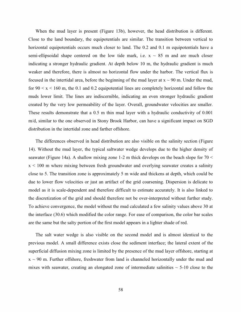
58

When the mud layer is present (Figure 13b), however, the head distribution is different.

Close to the land boundary, the equipotentials are similar. The transition between vertical to

horizontal equipotentials occurs much closer to land. The 0.2 and 0.1 m equipotentials have a

semi-ellipsoidal shape centered on the low tide mark, i.e. x ~ 85 m and are much closer

indicating a stronger hydraulic gradient. At depth below 10 m, the hydraulic gradient is much

weaker and therefore, there is almost no horizontal flow under the harbor. The vertical flux is

focused in the intertidal area, before the beginning of the mud layer at x ~ 90 m. Under the mud,

for 90 < x < 160 m, the 0.1 and 0.2 equipotential lines are completely horizontal and follow the

muds lower limit. The lines are indiscernible, indicating an even stronger hydraulic gradient

created by the very low permeability of the layer. Overall, groundwater velocities are smaller.

These results demonstrate that a 0.5 m thin mud layer with a hydraulic conductivity of 0.001

m/d, similar to the one observed in Stony Brook Harbor, can have a significant impact on SGD

distribution in the intertidal zone and farther offshore.

The differences observed in head distribution are also visible on the salinity section (Figure

14). Without the mud layer, the typical saltwater wedge develops due to the higher density of

seawater (Figure 14a). A shallow mixing zone 1-2 m thick develops on the beach slope for 70 <

x < 100 m where mixing between fresh groundwater and overlying seawater creates a salinity

close to 5. The transition zone is approximately 5 m wide and thickens at depth, which could be

due to lower flow velocities or just an artifact of the grid coarsening. Dispersion is delicate to

model as it is scale-dependent and therefore difficult to estimate accurately. It is also linked to

the discretization of the grid and should therefore not be over-interpreted without further study.

To achieve convergence, the model without the mud calculated a few salinity values above 30 at

the interface (30.6) which modified the color range. For ease of comparison, the color bar scales

are the same but the salty portion of the first model appears in a lighter shade of red.

The salt water wedge is also visible on the second model and is almost identical to the

previous model. A small difference exists close the sediment interface; the lateral extent of the

superficial diffusion mixing zone is limited by the presence of the mud layer offshore, starting at

x ~ 90 m. Further offshore, freshwater from land is channeled horizontally under the mud and

mixes with seawater, creating an elongated zone of intermediate salinities ~ 5-10 close to the

59

surface that progressively increase at depth to reach 30 salinity under 15 m below the mud

bottom.

This is in agreement with the observations made in Stony Brook Harbor, where an offshore

piezometer well recorded a salinity of 8 at x ~150 m and z ~ 15 m. Manual seepage meters

implanted in offshore muddy areas recorded the presence of freshwater, and the ultrasonic

seepage meters located in areas without mud layers displayed very high rates. This agrees with

both the salinity distribution predicted by the model and the strong vertical hydraulic gradient

under the mud.

6. Conclusion

A simplified 2D steady-state model of Stony Brook Harbor shows that a low permeability

mud layer as thin as 0.5 m is enough to significantly affect SGD distribution and composition.

The numerical predictions are in good agreement with salinity observations collected in the field.

The next step of this work would be to develop a transient model by including a dynamic

boundary condition for tidal sea level variations. This would allow more direct comparisons

between numerical predictions and electrical resistivity sections, piezometer salinity data and

seepage meter measurements in the intertidal zone. Several factors may result in the discrepancy

between field observations and numerical results, such as unsaturated flow and sediment

compressibility in tidal marshes [Gardner and Wilson, 2006; Wilson and Gardner, 2006], local

variations of porosity in sediments due to marshes roots and bioturbation. A sensitivity analysis

of the mud layer characteristics, i.e. thickness and permeability would help determine in which

conditions the mud layer can be neglected and when it is crucial to include it in SGD studies.

Porewater chemical analyses performed at our two sites identified two regimes of

denitrification linked to SGD flowpaths: discharge through the sandy sediments or through the

mud layer. It should be possible to couple the transport simulation to a particle tracking

algorithm that would provide a better understanding of the flow paths and residence time of

nutrients carried by the inland freshwater. This could help understand the nutrients fluxes into

the harbor and validate the hypothesis on nitrate fate [Young, 2013].

60

Future work will include the development of a 3D model that will enable the simulation of

the impact of the mud layer, the concave shoreline and the density-driven phenomena. By

including sediment heterogeneities, shoreline concavity and density-driven phenomena with

numerical modeling, the results of this study will highlight the fundamental differences between

the functional discharge mechanisms of coastal embayments with respect to ocean shorelines.

Improved quantification of SGD in coastal embayments will allow for more improved nutrient

mass balances. This methodology can be applied to any shallow, low-energy environment with

significantly differing surficial sediment regimes. A cohesive, regional modeling approach would

serve as an excellent complement to thermal infrared remote sensing techniques, allowing

researchers to better locate and quantify SGD on a larger scale, where field measurements may

be limited and/or not logistically practical [Johnson et al., 2008; Kelly et al., 2013].

61

References



Badon-Ghyben, W. (1888), Notes on the probable results of well drilling near Amsterdam,

Tijdschrift van het Koninklijk Inst. van Ing. Den Haag, 21.



Beck, A. J., Y. Tsukamoto, A. Tovar-Sanchez, M. Huerta-Diaz, H. J. Bokuniewicz, and S. A.

Sañudo-Wilhelmy (2007b), Importance of geochemical transformations in determining

submarine groundwater discharge-derived trace metal and nutrient fluxes, Applied Geochemistry,

22(2), 477-490.











Cooper Jr, H. H. (1959), A hypothesis concerning the dynamic balance of fresh water and

salt water in a coastal aquifer, Journal of Geophysical Research, 64(4), 461-467.




437.

Gibbes, B., C. Robinson, L. Li, D. Lockington, and H. Li (2008a), Tidally driven pore water

exchange within offshore intertidal sandbanks: Part II numerical simulations, Estuarine, Coastal

and Shelf Science, 80(4), 472-482.

Gibbes, B., C. Robinson, H. Carey, L. Li, and D. Lockington (2008b), Tidally driven pore

water exchange in offshore intertidal sandbanks: Part I. Field measurements, Estuarine, Coastal


62



Guo, W., and C. D. Langevin (2002), User's Guide to SEWAT: A Computer Program for

Simulation of Three-Dimensional Variable-Density Ground-Water Flow, United States

Geological Survey.

Harbaugh, A. W., E. R. Banta, M. C. Hill, and M. G. McDonald (2000), MODFLOW-2000,

the US Geological Survey modular ground-water model: User guide to modularization concepts

and the ground-water flow process, US Geological Survey Reston, VA, USA.

Heiss, J. W., W. J. Ullman, and H. A. Michael (2014), Swash zone moisture dynamics and

unsaturated infiltration in two sandy beach aquifers, Estuarine, Coastal and Shelf Science, 143,

20-31.

Herzberg, D. (1901), Die wasserversorgung einiger nordseebäder.




Kelly, J. L., C. R. Glenn, and P. G. Lucey (2013), High-resolution aerial infrared mapping of

groundwater discharge to the coastal ocean, Limnol. Oceanogr.: Methods, 11, 262-277.








Langevin, C. D., W. B. Shoemaker, and W. Guo (2003), MODFLOW-2000, the US

Geological Survey Modular Ground-Water Model--Documentation of the SEAWAT-2000

Version with the Variable-Density Flow Process (VDF) and the Integrated MT3DMS Transport

Process (IMT), US Department of the Interior, US Geological Survey.

Lewandowski, J., K. Meinikmann, T. Ruhtz, F. Pöschke, and G. Kirillin (2013), Localization

of lacustrine groundwater discharge (LGD) by airborne measurement of thermal infrared

radiation, Remote Sensing of Environment, 138, 119-125.



63



233-236.



110-127.





Lett, 30(6), 1297.






Mulligan, A. E., and M. A. Charette (2006), Intercomparison of submarine groundwater

discharge estimates from a sandy unconfined aquifer, Journal of Hydrology, 327(3-4), 411-425.

Mulligan, A. E., C. Langevin, and V. E. A. Post (2011), Tidal Boundary Conditions in

SEAWAT, Ground Water.







Robinson, C., L. Li, and H. Prommer (2007a), Tide-induced recirculation across the aquifer-

ocean interface, Water Resources Research, 43(7), W07428.



Robinson, C., B. Gibbes, H. Carey, and L. Li (2007c), Salt-freshwater dynamics in a

subterranean estuary over a spring-neap tidal cycle, Journal of Geophysical Research, 112(C9),

C09007.

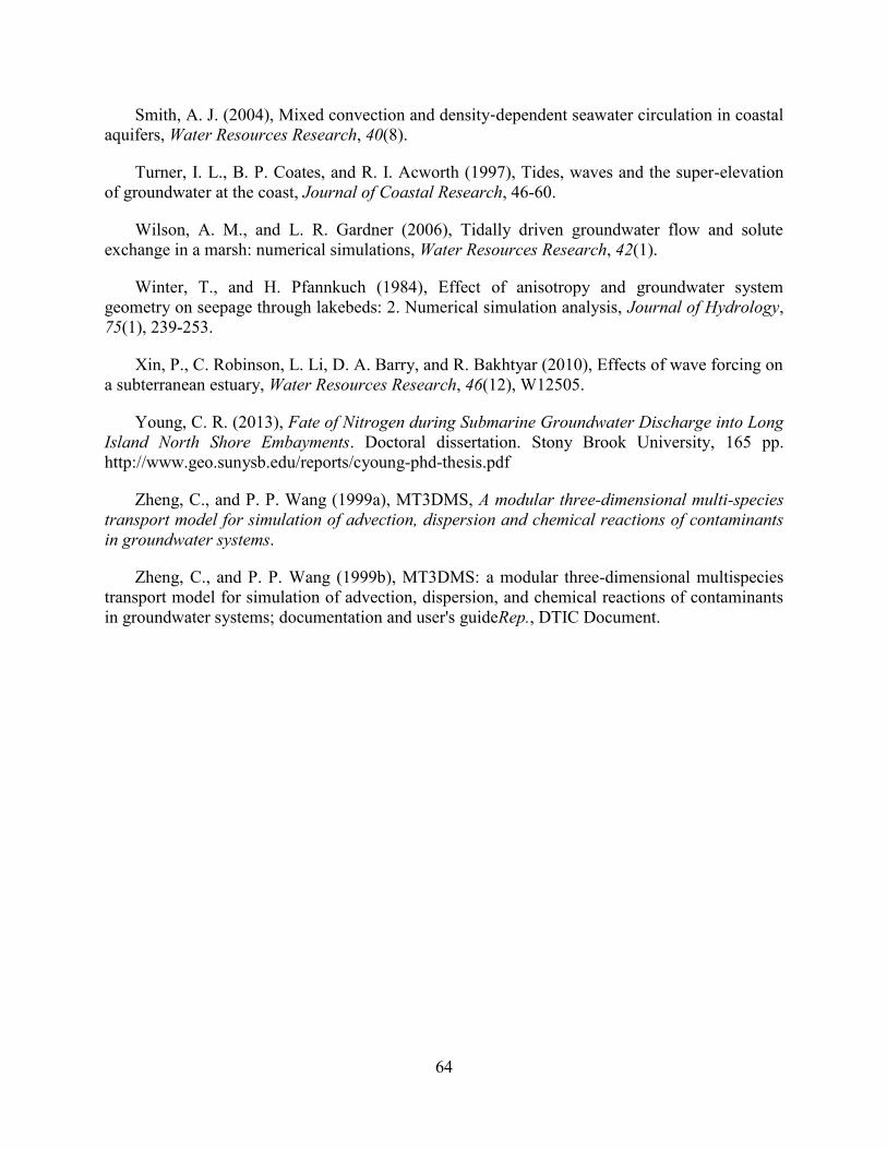
64

Smith, A. J. (2004), Mixed convection and density‐dependent seawater circulation in coastal

aquifers, Water Resources Research, 40(8).

Turner, I. L., B. P. Coates, and R. I. Acworth (1997), Tides, waves and the super-elevation

of groundwater at the coast, Journal of Coastal Research, 46-60.



Winter, T., and H. Pfannkuch (1984), Effect of anisotropy and groundwater system

geometry on seepage through lakebeds: 2. Numerical simulation analysis, Journal of Hydrology,

75(1), 239-253.





http://www.geo.sunysb.edu/reports/cyoung-phd-thesis.pdf

Zheng, C., and P. P. Wang (1999a), MT3DMS, A modular three-dimensional multi-species

transport model for simulation of advection, dispersion and chemical reactions of contaminants

in groundwater systems.

Zheng, C., and P. P. Wang (1999b), MT3DMS: a modular three-dimensional multispecies

transport model for simulation of advection, dispersion, and chemical reactions of contaminants

in groundwater systems; documentation and user's guideRep., DTIC Document.

65

Tables

Table 1. Stony Brook Harbor model parameters

Parameter Value Unit

Longitudinal dispersivity 0.5 m

Transversal dispersivity 0.05 m

Freshwater concentration 0.1 kg/m3

Seawater concentration 30 kg/m3

Constant head boundary 0.5 m

Diffusion coefficient 10-9

m2/d

Sand horizontal hydraulic conductivity 50 m/d

Sand vertical hydraulic conductivity 5 m/d

Mud horizontal hydraulic conductivity 0.001 m/d

Mud vertical hydraulic conductivity 0.001 m/d

Sand porosity 0.4

Mud porosity 0.62

Mud layer thickness 0.5 m

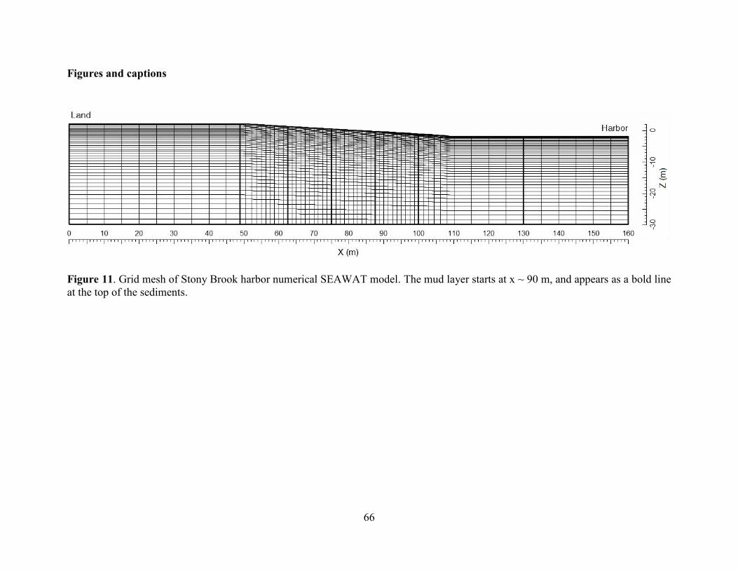
66


Figure 11. Grid mesh of Stony Brook harbor numerical SEAWAT model. The mud layer starts at x ~ 90 m, and appears as a bold line

at the top of the sediments.

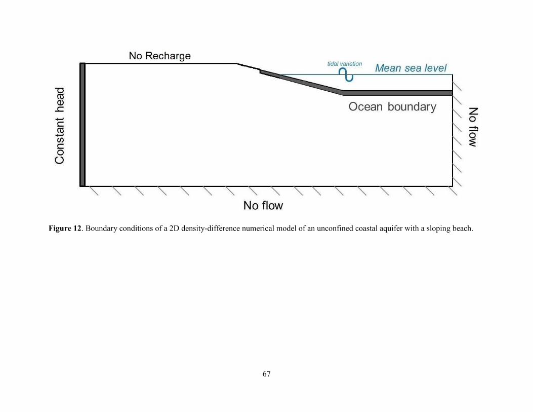
67

Figure 12. Boundary conditions of a 2D density-difference numerical model of an unconfined coastal aquifer with a sloping beach.

68

Figure 13. Equipotential distribution (in m) for Stony Brook Harbor steady state model without (a) and with (b) the low-permeability

mud layer, shown as the bolded black line.

69

Figure 14. Salinity distribution for Stony Brook Harbor steady state model without (a) and with (b) the low-permeability the mud

layer, plotted as a black bold line.

70

Chapter 4: Time-lapse electrical resistivity survey of the intertidal zone and implications

for submarine ground water discharge

Abstract

Submarine groundwater discharge (SGD) is now widely recognized as a crucial contributor

to surface water as it provides a pathway for nutrients and contaminants that can significantly

impact coastal ecosystems. Field measurements in the vicinity of the freshwater-seawater

interface (FSI) have shown that the spatio-temporal distribution of SGD can be highly

heterogeneous. Some numerical models have identified three regions (a density-driven

circulation cell offshore, an upper saline plume and a freshwater tube in the intertidal zone)

which seem to persist over time, such that the distinct regions can be recognized in simulations

that average the numerically predicted salinity profiles over the tidal phases. For each region, the

size and shape are influenced by factors such as the tidal and wave loading, inland hydraulic

gradient, beach geometry and aquifer properties. There is a paucity of field data about the

evolution of the salinity profile in the shallow regions of the FSI during a tidal cycle. To

characterize the spatio-temporal heterogeneities of the FSI and compare with numerical

predictions, I used electrical resistivity as a proxy for salinity. Electrical resistivity surveys were

acquired during a 12-hour cycle in a tidally dominated environment. My measurements indicate

fundamentally different scenarios during high and low tide. At low tide, the resistivity data

suggest an influx of freshwater from land, forming a plume that rises up and contributes

substantially to SGD in the intertidal zone. I also observed the occurrence of three regions

somewhat analogous to the numerical predictions. However, at high tide, instead of these distinct

regions, I observed a diffuse mixing zone that extended along the water/sediment interface and

overlaid the freshwater from land. Point measurements of seepage rates and salinity are in basic

agreement with the two scenarios. It should also be noted that the phase-averaged section

obtained with the resistivity surveys resembles the high tide resistivity end-member and therefore

differs from the phase-averaged simulations.

71

1. Introduction

The most general definition of submarine groundwater discharge (SGD) includes any

fluid crossing the sediment/ocean interface, regardless of its origin, driving-force and

composition [Burnett et al., 2003]. Understanding SGD is crucial to quantify chemical fluxes

from coastal aquifers to the ocean and to monitor seawater intrusion [Zektser et al., 2006]. SGD

provides a pathway for terrestrially-derived contaminants to reach the oceans and impact marine

ecosystems [Johannes, 1980] by altering coastal nutrient dynamics [Beck et al., 2007b]. The

mixing of fresh and salt porewater creates geochemically active zones that modify chemical

fluxes [Moore, 1999; Moore and Shaw, 1998; Valiela and Delia, 1990]. SGD importance is

widely recognized; nevertheless challenges intrinsic to its study persist. Due to its widely

distributed and heterogeneous nature, and its spatio-temporal variations at a variety of scales,

SGD remains difficult to quantify [Michael et al., 2003]. To address this issue many methods

have been developed [Burnett et al., 2006].

A variety of seepage meters are available to measure SGD directly. However, to

characterize the high spatial variability requires a large number of point measurements

[Bokuniewicz, 1980; Michael et al., 2003; Russoniello et al., 2013], or a combination of several

complementary methods [Burnett et al., 2006]. Numerical models have significantly contributed

to predicting SGD patterns for given conditions, and recent simulations have brought new

insight into flux dynamics and chemistry in coastal settings [Ataie-Ashtiani et al., 1999; Kuan et

al., 2012; Li et al., 1999; Robinson et al., 2006]. Numerical models have identified three distinct

hydrological regimes: a density-driven circulation cell offshore, a superficial intertidal saline

zone, and a freshwater discharge area between the two. The freshwater-seawater interface (FSI)

may fluctuate both in space and time due to variations in tides, waves or hydraulic gradient,

among others. While the three regimes and the FSI have been extensively studied over various

time scales in numerical simulations [Robinson et al., 2007a; Robinson et al., 2007b; Robinson et

al., 2007c], there is still a paucity of field data, especially regarding to the shallow processes and

their dynamics over a tidal cycle.

The main goal of this study is to elucidate these processes and the associated variations of

porewater salinity distribution in the intertidal zone of a sandy coastal aquifer, in West Neck Bay

(Shelter Island, NY) during a semi-diurnal tidal cycle. This study combines stationary time-lapse

electrical resistivity (ER) surveys of the intertidal zone and direct seepage measurements at the

72

sediment/ocean interface in the intertidal and subtidal zones. Salinities measured in the seepage

meters are compared to the fluid distribution imaged by the ER surveys, used as proxy for

salinity. SGD in West Neck Bay has been extensively studied in a comparative experiment led

by working group 112 of the Scientific Committee on Oceanic Research (SCOR) [Anonymous,

2002; Burnett et al., 2006; Dulaiova et al., 2006; Paulsen et al., 2004; Sholkovitz et al., 2003;

Stieglitz et al., 2008b; Stieglitz et al., 2007] and in other previous studies [O'Rourke, 2000;

Paulsen et al., 1998]. Some data suggested the existence of a confining unit at that site, but its

extent and properties were not characterized [Stieglitz et al., 2007]. A secondary goal of this

study is to investigate if deeper ER vertical cross-sections can image the extent of the postulated

confining layer.

2. Study Site

West Neck Bay is a small embayment located in the southwestern part of Shelter Island,

situated between the North and South forks of Long Island, NY, in the Peconic Estuary (figure

1). My study site was identical to the one chosen by the working group 112 of the Scientific

Committee on Oceanic Research (SCOR). The bay area is approximately 1 km2 and its depth

varies between 2 and 4 m [Gobler and Sañudo-Wilhelmy, 2001]. The bay exchanges water with

the Peconic Estuary through a narrow channel called West Neck Creek.

Shelter Island is a relatively simple hydrologic system as there are no significant streams,

and therefore all water entering the Peconic Estuary comes from overland run-off and

groundwater [Soren, 1978]. About half of the precipitation on Shelter Island is estimated to be

lost by evaporation; the remaining 5% reaches the estuary as run-off, making groundwater the

major contributor of freshwater.

Shelter Island is composed of upper Pleistocene deposits of glacial drifts consisting of

clay, silt, outwash sand and gravel, cobbles and boulders [Soren, 1978]. These deposits constitute

the Upper Glacial Aquifer, under which lays two distinct confining clay units, the Magothy

aquifer, the Raritan clay and the Lloyd aquifer. Fresh groundwater is limited to the upper glacial

aquifer, as revealed by exploratory drilling. The clay confining unit and the deeper aquifers

contain saline water. Thickness of the upper glacial aquifer varies between 23 and 33 m at

73

Shelter Island. More details about the geology of the island can be found in [Schubert, 1998;

Soren, 1978].

On Shelter Island, hydraulic conductivities range from 60 to 83 m/d, the average porosity

is 30% and the hydraulic gradient 0.00115 [Soren, 1978]. The anisotropy ratio in the upper

glacial aquifer on Long Island was inferred to be 10:1 from numerical modeling [Buxton and

Modica, 1992]. The saltwater interface is located at about 15 m under sea level, as inferred from

geochemical data [Gobler and Sañudo-Wilhelmy, 2001].

The shore around West Neck Bay is mainly composed of coarse-grained sand and gravel

and has slope of 1:8 (or 7.1°) [Paulsen et al., 2004]. The average salinity in the bay is

approximately 26, but was approximately 31 during my study. The average tidal range is around

1.2 m but was measured to be 0.8 m during our data acquisition. Due to the shape of the bay,

wave influence is negligible.

3. Methods

The intertidal zone was studied using four different techniques: stationary time-lapse

electrical resistivity (ER) surveys providing 2D vertical cross-sections repeated over time, point

measurements of conductivity and temperature using a Trident probe, manual and automated

seepage measurements, and fluid parameter analysis using a YSI 556 multiprobe hand meter.

Each method is described in the following sections; experimental setup is outlined in Figure 2.

3.1 Electrical resistivity survey acquisition and processing

Because electrical resistivity of fluids in coastal settings can vary up to six orders of

magnitude, its spatial distribution provides a useful proxy for fluid mixing and dynamics

underground. However, the relation between measured bulk resistivity and pore water salinity is

not straightforward. The inverted resistivity of saturated sediments from field data and its spatial

variation is a function of the geometry of the acquisition setting, salinity, saturation, clay content

and porosity [Olhoeft, 1981]. The electrodes in most of the intertidal zone were located in fully

saturated sediments as indicated by the observed seepage face during ebbing and low tide.

Consequently, in the intertidal and subtidal zones, the changes in conductivity can be attributed

solely to the electrolyte conductivity and therefore be used as a proxy for salinity [Telford et al.,

1990]. Higher ER would indicate relatively lower salinities due to the influx of fresh SGD

74

[Swarzenski et al., 2007]. The electrodes of the landward portion of the survey located above the

high tide mark were coupled with partially saturated sediments, but were not the focus of the

present study so no computation of fluid properties were made for this portion of the transect.

ER imaging was performed using an Advanced Geosciences Inc. (AGI) SuperSting 8-

channel receiver R8 resistivity meter. The SuperSting system uses a 56 electrode cable with 0.61

m electrode spacing. One preliminary stationary survey was acquired on 09/12/2012 at low tide.

The cable was placed perpendicularly to the shore, 4 m northward of the pier, and independent

C/T measurements were taken with the Trident probe to assess the reliability of the inversion. On

09/13/12 a 12 hour time-lapse survey was performed at the same location, with transects named

A to L, during a semi-diurnal tidal cycle from high tide to the next high tide (Figure 16b). The

cable was placed partially on land and partially in the water. All electrodes on land and in the

intertidal zone were linked to the ground through springs attached to 0.3 m metallic stakes to

ensure good coupling. A mix of swelling bentonite clay and seawater was poured on each land

electrode to maximize surface contact with the ground. Exposed electrodes were wet with

seawater at the beginning of each ER survey.

Measurements were made using a combination of dipole-dipole and Schlumberger

configurations to optimize both vertical and lateral resolutions, and the data were stacked

together for the inverse analysis. Data were analyzed using the software package EarthImager

2D [AGI, 2009]. Several 2-dimensional finite elements inversion methods are available: a

damped least square inversion, a robust inversion that enables relatively sharp contrasts as the

distribution of data errors is assumed to be exponential, and a smooth inversion, called Occam’s

inversion [Constable et al., 1987], that assumes a Gaussian error distribution. All methods were

tried; the smooth inversion was selected as it minimized the appearance of artifacts that cannot

be real as they are smaller than the resolution of the survey.

Two parameters allow estimating the quality of the inversion: the room mean square error

(RMSE) and the Euclidian norm (L2). Both are statistical measures of the residual difference

between the inverted model and the data. Typically, a RMSE under 10 % and/or a L2<1 indicate

a good fit between the inverted model and the measurements.

Water depth and fixed seawater resistivity values can strongly influence the result of the

inversion [Day-Lewis et al., 2006; Henderson et al., 2010]. Preliminary data analysis revealed

that fixing the water column resistivity prevented convergence of the model no matter which

75

inversion technique or initial model was used. Water resistivity was therefore not constrained in

our inversion.

The land topography and bathymetry along the profiles were carefully measured using a

laser station and a sonic depth sounder, respectively. Water levels were continuously monitored

using a Solinst pressure logger to determine tidal depth variations for each individual transect.

Inversions were performed using the average water depth measured during acquisition. A

sensitivity analysis indicated that water level variation smaller than 0.25 m during data

acquisition would not produce significant artifacts in the inverted section when the water

resistivity is left unconstrained [Durand et al., 2011]. This amplitude of variation was not

attained for any of the 12 ER time-lapse surveys. For easier comparison between resistivity

surveys, Trident measurements and YSI readings, the resistivity sections were converted to

conductivity sections. One must also keep in mind that the inverted section represents an optimal

estimation of the spatial distribution of resistivity on the vertical profile and that the solution is

non-unique [Tarantola, 2005]. Comparing ER survey results with another method is therefore

necessary to provide confidence to the ER interpretation.

3.2 Seepage meters

SGD at selected locations was quantified using an ultrasonic seepage meter, for which

detailed description is available in [Paulsen et al., 2001]. SGD was captured in a steel collection

chamber (with a square cross section of 0.21 m2) inserted approximately 10 cm into the

sediment. The discharge was directed to a cylindrical flow tube with two piezoelectric

transducers that continually generate bursts of ultrasonic signals in opposite directions (periodic

waves with a frequency of 1.7 MHz). Arrival of the ultrasonic signals was continuously

monitored and allows determination of the flow direction and instantaneous velocity. The meter

is capable of measuring SGD at rates as low as 0.86 cm/d, with a sampling period as high as 5

minutes during several days.

Two ultrasonic seepage meters U1 and U2 were deployed between 9/11/12 and 9/14/12 at

19 and 23 m from the high tide mark, respectively, in alignment with the electrical resistivity

surveys (Figure 16a). Measurements were taken every 5 minutes for 4 days. Two Solinst loggers

were placed inside the funnels to measure SGD temperature and conductivity as well as real time

tidal level with a 5 minute sampling period.

76

In addition, 2 manual seepage meters [Lee, 1977] M1 and M2 were deployed on

8/14/2012, at 4 and 7 m from the high tide mark, respectively (Figure 16a). SGD rates were

measured and water samples collected for 10 hours during the time-lapse resistivity survey, to

measure temperature, conductivity and salinity.

3.3 Trident probe

The Trident probe is a direct-push instrument, developed to screen and assess offshore areas

where groundwater may be discharging to the surface water body [Chadwick et al., 2003]. The

probe integrates two temperature sensors, two electrical conductivity sensors, and two pore water

samplers. The subsurface C/T probe measures the electrical conductivity and temperature of the

sediments at a chosen depth, whereas the surface C/T sensors measure the electrical conductivity

and temperature of the surface water above the sediment-water interface. In this study, the depth

was fixed at 0.6 m below the sediment-water interface, but it represents the maximum depth

attainable as sediments sometimes did not allow full penetration. The temperature sensor has a

measurement range of -5 to +35 °C with an accuracy of 0.001 °C, and a resolution of 0.00025

°C.

The Trident probe was used to provide independent instantaneous measurements to ground-

truth the inversion from a preliminary study, the day before the 12h time-lapse survey. Four

tridents points were chosen along the survey line and the conductivities were measured at ~0.4 m

depth.

3.4 Salinity measurements

Water collected from the seepage meter and the Trident pore water were analyzed for

temperature, conductivity and salinity using a YSI 566 handheld multiprobe. Characterizing the

actual pore water seeping through the sediment-ocean interface aid in confirming the results

from the ER surveys.

Although the Solinst loggers placed in the ultrasonic seepage meters did record temperature

variations, the conductivity sensors did not. It is still possible to compute SGD salinity with the

Coppens equation [Coppens, 1981] using the instantaneous speed of sound recorded by the

piezoelectric transducers, the instantaneous temperature and depths from the logger:

77

( ) ( ) ( ) ( )

[ ( )]( ) (Equation 1)

with:

( ) ( )( )

- t = T/10, where T = temperature in degrees Celsius

- S = salinity in parts per thousand

- D = water depth in kilometers

This equation was developed for temperatures between 0 and 35 °C, salinities between 0 and 45,

and depths between 0 and 4 km.

4. Results

4.1 Electrical resistivity surveys and Trident probe

Two methods are used to assess the reliability of the inverted sections. First, the ER section

acquired on 9/10/13 is plotted against the conductivity measurements obtained with the trident

probe (Figure 17), after conversion to a fluid conductivity section using a formation factor of 3.3

calculated by Paulsen et al. [2004], which is compatible with a sand porosity of 30% and a

cementation factor of 1.3, typical of unconsolidated sands [Archie, 1942]. There is a good

agreement between the two independent data sets; the Trident measurements in the intertidal

zone are slightly higher than the inverted values. This could be the result of pore water

temperature variations measured by the Trident but ignored by the ER survey, or an artifact of

the level of detail created by the interpolation technique used to plot the inverted section. A

perfect match is not expected due to the nature of the comparison; agreement within an order of

magnitude is satisfactory.

Another method of estimating the reliability of the inversion is to compare the results

obtained for different initial conditions [Oldenburg and Li, 1999]. Inversions were performed

with three initial models to compare the stability of the inversion (Figure 18). The RMSE and L2

values were 7.79% and 0.59, 16.57% and 0.52 and 8.13% and 0.58 for the pseudosection, the

average apparent resistivity and the custom resistivity, respectively. The overall results are

consistent between methods and do not show any excessive difference at high depths, which

78

indicates that the inversion is stable over the whole thickness of the section [Oldenburg and Li,

1999]. The amount and position of resistive and conductive features are similar, however, the

absolute resistivity values vary between methods. This shows that, for this setting, resistivity can

be used to image contrasts and changes in subsurface resistivity but is not the most appropriate

tool to give an accurate estimate of salinity distribution. However, the use of the apparent

resistivity pseudosection as an initial model creates high frequency artifacts after inversion

visible on Figure 18(a) for 15 < x < 27 m. This inversion seems more sensitive to the noise in the

data and was therefore not used further on. The overall RMS and L2 values of the inversion with

the average apparent resistivity model were lower and this method was therefore chosen for the

time-lapse inversion. In spite of the care taken to ensure the minimum amount of noise during

acquisition, all sections had to be filtered and about 20% of all data sets were removed.

The results of the 12 time lapse ER surveys conducted during a semi-diurnal tidal cycle are

shown in (Figure 19 and Figure 20). Previous studies suggest that the aquifer is not

homogeneous in this area and suggested the presence of a confining unit [Stieglitz et al., 2007] or

clay lens [Paulsen et al., 2004]. Interpretation of bulk conductivity measurements in term of pore

fluid composition must therefore be done with caution. However, lithology and porosity are

constant over time and therefore comparing transects at different times still provides information

about the pore fluid composition.

At high tide, on transect A, a low conductivity sub-horizontal cell is observed originating

from land and extending to almost 20 m in the horizontal direction and down to z ~ -2 m depth

(Figure 19). A layer of approximately 1 m thickness with high conductivity is observed from the

high tide mark to the end of the profile. At depth, for x ~ 32 m a region of intermediate

conductivities is observed extending from the surface to z ~ -5 m. This could be part of the

mixing zone formed by the saltwater wedge or just an edge-effect, an artifact of the inversion.

Profile B is very similar to profile A, with the development of a low conductivity feature at x ~

25 m and -6 < z< -4 m. This feature does not persist on the following sections but reappears

more clearly before the next high tide stage on sections I and J. On profile C, the resistivity cell

seems less visible and fingering of intermediate conductivities develops in the middle of the

section. In D, the resistive cell is in contact with the top of the sediments close to the high tide

mark, at x ~ 10 m; fingering is amplified. On transect E, the resistive cell looks more continuous

and the portion in contact with the sediment interface is growing. A superficial mixing cell forms

79

landward of the contact point with the sediments. Some high frequency features appear between

x = 15 and x = 20 m which are the results of noise in the inversion due to the rapid change in

water level. Part of the fingering appears sub horizontal at about -2 m depth. This could be an

artifact due to the low conductivity of the feature above preventing adequate penetration of the

signal, but the low underlying resistivity contradicts this interpretation. The land resistive

structure is now developing a tube-like feature at depth under 4 m that reaches as far as 23 m.

The low tide profile F (Figure 20) confirms the structure shown in E. The resistive cell in contact

with the sediment interface is becoming wider, almost reaching the low tide mark. In G, the

resistive cell reaches its maximum extent, between x = 0 and x = 26m. The superficial mixing

cell widens as the tide retreats, but its depth remains very limited. The sub horizontal conductive

structure persists until transect J, before the next high tide. This structure could be the results of

partially confining clay until described by Stieglitz et al. [2008b]; however, the fact that the

structure disappears at high tide rules out the presence of the clay unit(DOI index > depth of

structure). The tube like portion of the resistive cell appears to move vertically on transect J, at

x~25 m, but does not reach the surface. The two parts of the resistivity cell on transect J surround

a more conductive structure, which resembles the model from Robinson et al. [2006] with a

freshwater tube and the upper saline plume. However, the structure is not permanent as simulated

by Robinson et al. [2006]. High tide profiles K and L look like the initial high tide transect A.

The ER sections reveal dynamic flow patterns in the intertidal and subtidal zones, as observed by

Befus et al. [2013].

Published numerical simulations present salinity distributions that are averaged over a tidal

cycle [Gibbes et al., 2007; Robinson et al., 2006; Robinson et al., 2007a; Robinson et al., 2007b].

For comparison, I computed the tidal average of all sections (Figure 21c), a high tide average

using the profile A, B and L (Figure 21a) and a low tide average using the profiles F, G and H

(Figure 21b). The tidal average looks like the high-tide end-member (Figure 21a), which

significantly differs from the numerical predictions. The low-tide end-members (Figure 21b) is

closer to the numerical predictions with three zones: a superficial mixing cell centered about the

high tide mark 5 < x < 10 m and 0 < z < 1 m, a resistive cell originating from land and exiting at

the sediment interface in the intertidal zone and finally a diagonally oriented zone with

intermediate conductivities that could resemble the upper saline plume, the freshwater discharge

tube and the saltwater wedge, respectively, as described in [Gibbes et al., 2007; Robinson et al.,

80

2006; Robinson et al., 2007a; Robinson et al., 2007b]. There are, however, some discrepancies in

shape and position of these features between the observations and the model results, as discussed

in section 5.

The high-tide end-member indicates a strong freshwater signal from land, but the

resistive cell is sub horizontal and extends at depth a couple of meters beyond the low tide mark.

The cell does not reach the sediment interface. The freshwater signal persisted over time and was

visible at low tide, but seems to be in direct contact with the sediment surface. The zone of

contact imaged on the ER sections coincided with a freshwater seepage face identified by

rivulets at the surface [O'Rourke, 2000], and included the locations of both manual seepage

meters. Salinity of water from the seepage face was measured at 0.2.

4.2 SGD in the intertidal zone: manual seepage meters

Specific discharge measured with the manual seepage meters are presented in Figure 22.

Seepage rates were very high, varying from 40 to 145 cm/d with an average of 93 cm/d for M1,

and varying from 12 to 74 cm/d with an average of 38 cm/d for M2 during the period recorded.

Unfortunately, it is not possible to obtain continuous SGD measurements at the intertidal zone,

as the seepage meters cannot record data if the water column thickness is insufficient for the bag

to float or if the meter is exposed, as shown by the gap in data around low tide. SGD in seepage

meter M1 did not exhibit a clear trend relative to the tide; M2 showed higher SGD rates around

low tide. In both meters, salinity measurements indicate a progressive freshening from high tide

to low tide with initial salinities equal to that of the bay at 33. After the gap in data, salinities in

the collection bags average 2 and 7 in A and B, respectively. In seepage meter A, there was a

progressive increase in salinity with flooding tide, starting at 0.62 after low tide to 5.2 before

high tide. In seepage meter B, the salinity was 6.66 after low tide and increased slightly to 7.2

before high tide.

Conservation of mass in the seepage meter can be described as follow:

(Equation 1)

With and

the mass of salt contained in the manual seepage meter at time t+1 and t,

respectively; the mass of salt entering the seepage meter through SGD at time t+1, and

the mass of salt exiting the seepage meter via the collection bag at time t+1.

81

We have , with m the mass of salt (g), S the salinity (g/L) and V the volume (L).

Under the hypothesis of an incompressible fluid, we have

and Equation

1 becomes:

(

) (Equation 2)

If we assume that there is full mixing in the seepage meter and that the salinity in the bag

is equal to the salinity in the seepage meter, i.e.

then we can rearrange equation 2

into equation 3:

(

)

(Equation 3)

All quantities on the right-hand side of the equation were measured and it is therefore

possible to remove the artifact due to the dilution of surface water trapped during the seepage

meter installation and to compute the salinity of SGD (Figure 23b). Assuming conservative

mixing, a freshwater salinity of 0.1 (Jonathan Wanlass, pers. comm.) and a surface water salinity

of 33, measured by a YSI probe, it is possible to estimate the percentage of freshwater contained

in SGD and in the collection bag (Figure 23).

For both seepage meters, the initial salinity measured in the collection bags is close to the

bay, 31, which corresponds to almost 98% of seawater. As the water level decreases, so does the

salinity. The rates of freshening are very similar for both seepage but after low tide the

percentage of freshwater is approximately 98 % in seepage meter A versus 80% in B. The

decrease in freshwater content observed in seepage meter A is absent in B.

The computation of SGD salinity and freshwater content according to equation 3 are

presented in Figure 23b. Computed SGD salinities in A are close to 20 corresponding to 66% of

freshwater and decrease slowly towards low tide. After low tide, SGD salinity is approximately

10 and increases quickly. High-frequency oscillations are visible before low tide and are even

stronger after low tide. Some computed salinities for A and SGD salinities for B are negative

which is unreliable. Possible explanations for these observations are presented in the discussion,

section 5b.

4.3 SGD in the subtidal zone: ultrasonic seepage meters

Ultrasonic seepage meter (USM) U1, located at 19 m form the high tide mark, recorded

both positive and negative fluxes that correspond to discharge and seawater infiltration,

82

respectively. SGD varies between -80 and 28 cm/d with an average of -7 cm/d and a clear

correlation with the tide is visible, as observed in previous studies [Anonymous, 2002; Paulsen et

al., 2004; Taniguchi, 2002]. A peak in tide is followed by strong seawater infiltration and a low

tide is followed by a positive discharge. An observed delay of ~ 1h has been previously

characterized by Paulsen et al. [2004]. Salinities computed using Coppens equation [Coppens,

1981] are approximately 12 with variation less than 1. This indicates a 60% freshwater content

using the bay water and the well water as salinity end-members. The minimum salinity values

were attained during rising tide when positive SGD reached its maximum. A diurnal signal is

clearly visible on the salinity curve. The peaks coincide with the warmer air temperatures

between 9 am and 6 pm and reveal the influence of temperature on the salinity computation

(equation 1).

USM U2, located at 23 m from the high tide mark, did not measure any discharge from

the sediments to the ocean but only seawater infiltration as indicated by the strictly negative

values. SGD varies between -20 and -9 cm/d with an average of -13 cm/d. There is no correlation

with the diurnal tidal signal marking the horizontal limit of the zone of tidal influence. Salinity is

high and similar to that of the bay. Diurnal peaks in salinity occur between 12 PM and 8 PM,

which is later than U1. The delay is probably due to the thicker water column above U2 that

delays the propagation of the heat signal.

The salinities differences measured in U1 and U2 are in good agreement with the pore

water composition inferred from the resistivity section. The constant negative discharge in U2

correlates with the position of higher conductivity features extending at depth, on the seaward

end of the profiles. The agreement between both data sets indicate that this feature is not an

edge-effect of the inversion, but is most likely the density driven circulation cell termed the salt-

water wedge [Kohout, 1960]. The density-driven circulation cell appears closer to land than

previously observed with bulk conductivity profiles at x ~ 45 m from the mean tide mark

[Paulsen et al., 2004].

5. Discussion

5.1 Comparison with other studies: SGD rates

A summary of SGD estimates in West Neck Bay is presented in Table 2. No

measurements were previously done in the intertidal zone but our values from the manual

83

seepage meters are in remarkable agreement with the ones performed by Paulsen et al. [2004] in

the subtidal zone. Values recorded by the ultrasonic seepage meter 19 m offshore of the high tide

mark are in good agreement with all other methods. I observed a decay in SGD rate with

increasing distance from the shore, and a negative correlation between SGD and tidal level, in

agreement with all previous observations [Anonymous, 2002].

My study, however, is the only one which recorded negative seepage values offshore,

indicating seawater intrusion. All experiments for the SCOR project were made in spring when

precipitations rates are high (35.3 cm cumulated from March-May 2002) and evapotranspiration

has not reached its peak yet whereas our data were acquired in fall (12.2 cm cumulated from July

to September 2012). The inland hydraulic gradient is relatively smaller during the fall season and

as suggested by numerical simulations, position of the freshwater-seawater interface varies

seasonally [Michael et al., 2005], which is in agreement with the location of the saltwater wedge

on our ER survey results.

As mentioned in [Stieglitz et al., 2008b; Stieglitz et al., 2007] such high SGD rates are

unusual in an unconfined aquifer and could be indicative of a confined or partially confined

aquifer.

5.2 Interpretation of SGD composition

The similar salinities measured in manual SM A and B at the beginning of the experiment

are significantly different from the salinities measured after low tide, in spite of nearly identical

freshening rates during ebbing tide. This suggests that the salinity variations in the seepage

chambers could be mostly due to the progressive dilution of seawater trapped during installation.

The lack of symmetry between salinities recorded at both high tide stages also point in this

direction. If a full seepage meter volume, i.e. 39 L, were to be pushed into the sediments during

installation, this volume would only be completely flushed after 6 h in A and 12 h in B thus

invalidating most of the salinity measurements. The manual seepage meters used are each

equipped with a 10 cm diameter rubber plug that is installed only after the chamber is inserted

into the sediments, in order to minimize the amount of seawater that can be trapped. The almost

constant salinities observed in the collection bag from B after only 6 h indicate that this scenario

is unlikely and show that, at least the salinities measured after low tide are not affected by the

dilution effect. The lack of symmetry between salinity can be a consequence of the incomplete

84

sampling time; we did not capture a full tidal cycle but 9.5 hours, if we exclude the first bag due

to seepage meter equilibration. If the rate of salinity increase observed in A during flooding tide

is constant, salinity would increase by 24 and reach 29, i.e. a freshwater content of 12% at the

end of the 12 hours; seepage meter B salinity would remain constant at 8 or 78% freshwater. The

increase in seawater content observed in A after low tide is much faster than the freshening

observed during ebbing tide. The beach saturates more easily than it drains, which is due to the

slope of the beach and the asymmetrical transient response of the inland hydraulic head to the

tidal stimulation, as predicted by an analytical model [Turner et al., 1997] and previously

observed at this site [Paulsen et al., 2004].

An attempt to derive SGD salinity and composition over time, using manual seepage

meters in the intertidal zone, yielded results that were not consistently interpretable. This

indicates that some of the assumptions made for the calculations were not justified. One

assumption was that the fluid was incompressible. Even if this is not entirely accurate, the

compressibility of water cannot account for the magnitude of errors observed. A second

hypothesis is that water in the seepage chamber is well mixed and that salinity measured in the

bag at a given moment is representative of the salinity inside the seepage meter at the same

moment. In spite of the density difference between fresh and sea waters, it is very unlikely that

any significant salinity layering could develop in such a small volume and short amount of time.

The last assumption states that the volume of SGD entering the seepage meter is equal to the one

collected in the bag. This can only be true if the flow is unidirectional. Prefilling the bags can

allow for groundwater recharge but is not recommended if water quality analyses are performed

[Libelo and MacIntyre, 1994; Shaw and Prepas, 1989]. We did not prefill the bags to avoid

introducing external water in the system and could therefore only record positive SGD. As the

bag volume is directly used in equation 3, it appears that unrecorded bidirectional exchanges of

flow and solutes within the seepage meters are responsible for the negative calculated salinity

values and complicate estimates of SGD composition.

West Neck Bay is a relatively wave-free environment. Hydraulic head oscillations

attenuate very rapidly at this site, a 90 % decay was observed between wells situated

approximately 50 m apart for a 12 hour period signal [Paulsen et al., 2004], hence higher

frequencies should attenuate even faster. The high-frequency oscillations observed in the

85

computed SGD salinities are not therefore not the results of waves and are most likely an artifact

of the bidirectional fluxes not accounted for in the calculations.

5.3 Impact of sediment heterogeneities on SGD

The ER cable was installed 4 m north of the jetty present at our site to avoid the

disturbance created by the perforation of a suspected but unconfirmed confining layer [Stieglitz

et al., 2007]. The seepage meters were placed 1 m north of the ER cable. The very high seepage

rates measured in the intertidal zone are similar to previous peak values obtained close to the pier

[Paulsen et al., 2004], and these high rates are consistent between spring and fall which is

consistent with the existence of a confining layer. However, the inferred depth of the confining

layer varied between 0.2 and 0.5 m which is deeper than the penetrating depth of the manual SM

of ~ 0.10 m. Surface bulk conductivities did not indicate any interruption in the confining layer

close to the shore [Paulsen et al., 2004]. If the layer restricts the vertical water exchanges, the

water collected in the intertidal zone might therefore come from lateral fluxes from the jetty,

which disagrees with the surface bulk conductivities suggesting that the influence of the jetty

extended farther laterally than previously thought. Yet, discharge rate predictions using an

analytical model for an unconfined anisotropic aquifer [Rumer and Shiau, 1968] were in

agreement with the observations even if tidal forcing was not accounted for [Paulsen et al.,

2004].

Surface bulk conductivity measurements in the subtidal zone indicated that the position

of the superficial mixing zone did not vary significantly between high and low tide [Stieglitz et

al., 2008b], which is in agreement with the results from our time-lapse ER survey.

5.4 Interpretation of ER time-lapse survey

In spite of some inherent limitations of the electrical resistivity method, our data suggest a

partial agreement with current numerical models developed for a homogeneous isotropic aquifer

[Robinson et al., 2006] and field measurements in unconfined sandy aquifers [Gibbes et al.,

2008b]. At low tide, 3 regions similar to the ones predicted by simulations, i.e. an upper saline

plume, freshwater tube and saltwater wedge are observed. However, there are some

discrepancies: our low tide end-member conductivity section resembles the published model,

however, a 12 hr. phase-average does not and is more similar to our high-tide end-member. The

86

shape and position of the FSI in the intertidal zone differ from the model. The intertidal shallow

mixing zone and the freshwater discharge area appear to be mobile. Several factors can explain

the apparent discrepancies between our data and the model: the curvature of the shoreline is

known to focus flow, the anisotropy and sediment heterogeneity of the aquifer, and 3D geometric

complexity due to the presence of the jetty.

Vertical movements of the fresh water discharge zone suggested by the ER sections are in

agreement with the salinity variations recorded in the manual seepage meters. The ER results,

however, do not confirm the presence of a confining unit as described by [Stieglitz et al., 2007].

In theory, clay formations are less resistive due to strong surface conduction [Archie, 1942;

Revil, 1998]. However, in coastal settings it is likely that conductivity occurs mostly in the

porous medium saturated with saline water. Furthermore, to be imaged by the ER survey a

feature needs a minimum contrast of 20 % between its resistivity and the surroundings, and its

dimensions must be larger than at least on spacing between electrodes, 0.6 m in our case. It is

therefore possible that the confining unit cannot be resolved by the ER survey. Nevertheless,

even if that layer is invisible on the cross-sections it should be possible to observe its

hydrological effects. Temporal variations in conductivity distribution down to 6 m below grade

do not seem to indicate any segregation between an upper and a lower portion of the aquifer.

Sub-horizontal movements do not appear to be favored by other factors than aquifer anisotropy

and no horizontal feature is sufficiently consistent over time to be interpreted as a structure in the

sediments. A confining unit thicker than 6 m would prevent SGD as high as measured.

6. Conclusion

The geophysical techniques used in this study did not find definitive evidence of the

existence of a confining unit as previously suggested; however, my data do not completely rule

out its presence either. High SGD rates found in the intertidal zone are in favor a partially

confined aquifer; however, the dynamic conductivity distribution at depth disagrees with the

presence of a continuous low permeability unit at depth. Core measurements are necessary to

determine the hydrogeological setting at this location. Numerical models for homogeneous

isotropic straight-beach aquifer cannot predict the observations, revealing the need for

anisotropic and heterogeneous models. This would enable us to better characterize flow and

87

solute transport that determine the biogeochemical reactions occurring in the subterranean

estuary and impact chemical fluxes associated with SGD.

88

References


Iversion Software, Austin, Texas, Report.


experiment, , International Hydrological Program (IHP), Scientific Commitee on Oceanic

Research (SCOR), Land Ocean Interactions in the Coastal Zone (LOICZ), Report, 26 pp.








22(2), 477-490.















289-300.

Coppens, A. B. (1981), Simple equations for the speed of sound in Neptunian waters, The

Journal of the Acoustical Society of America, 69(3), 862-863.

89







Durand, J. M., J. Wanlass, N. Stark, R. Paulsen, and T.-f. Wong (2011), Study of submarine

groundwater discharge on the west shore of Forge River using electrical resistivivty

measurements and seepage meters, paper presented at Geology of Long Island and Metropolitan

New York, 18th proceedings, Stony Brook, NY, USA, April 9th 2011.



884-894.






Gobler, C. J., and S. A. Sañudo-Wilhelmy (2001), Temporal variability of groundwater

seepage and brown tide blooms in a Long Island embayment, Marine Ecology Progress Series,

217, 299-309.




18(1), 173-185.












90



Libelo, E. L., and W. G. MacIntyre (1994), Effects of surface-water movement on seepage-

meter measurements of flow through the sediment-water interface, Applied Hydrogeology, 2(4),

49-54.



Lett, 30(6), 1297.







21552.




Brook.

O'Rourke, D., P. R., and W. T-f. (1999), Measuring Submarine Groundwater Seepage Using

an Ultrasonic Flow meter and the "Drum Method"- A Comparative study, in Geology of Long

Island and Metropolitan New York, edited, Stony Brook, NY, USA.




2, 298-305.









91

Revil, A. (1998), Nature of surface electrical conductivity in natural sands, sandstones, and

clays, Geophys Res Lett, 25(5), 691-694.









C09007.

Rumer, R. R., and J. Shiau (1968), Salt water interface in a layered coastal aquifer, Water

Resources Research, 4(6), 1235-1247.




Schubert, C. E. (1998), Areas contributing ground water to the Peconic estuary, and ground-

water budgets for the North and South forks and Shelter Island, Eastern Suffolk County, New

York.






Soren, J. (1978), Hydrogeologic conditions in the town of Shelter Island, Suffolk County,

Long Island, New York., Water-Resources Investigation Report Rep. 77-77, U. S. Geological

Survey.






543-550.



92


Technology, 41(20), 7022-7029.



Tarantola, A. (2005), Inverse problem theory and methods for model parameter estimation,

siam.


Pr.



VALIELA, I., and C. DELIA (1990), Special issue-groundwater inputs to coastal waters-

introduction, edited, Kluwer Academic Publ Spuiboulevard 50, PO Box 17, 3300 AA Dordrecht,

Netherlands.


Press Inc.

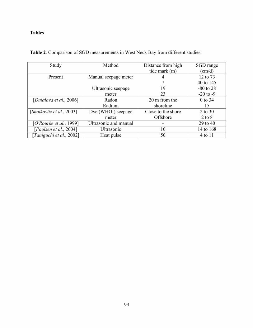
93

Tables

Table 2. Comparison of SGD measurements in West Neck Bay from different studies.

Study Method Distance from high

tide mark (m)

SGD range

(cm/d)

Present Manual seepage meter

Ultrasonic seepage

meter

4

7

19

23

12 to 73

40 to 145

-80 to 28

-20 to -9

[Dulaiova et al., 2006] Radon

Radium

20 m from the

shoreline

0 to 34

15

[Sholkovitz et al., 2003] Dye (WHOI) seepage

meter

Close to the shore

Offshore

2 to 30

2 to 8

[O'Rourke et al., 1999] Ultrasonic and manual - 29 to 40

[Paulsen et al., 2004] Ultrasonic 10 14 to 168

[Taniguchi et al., 2002] Heat pulse 50 4 to 11

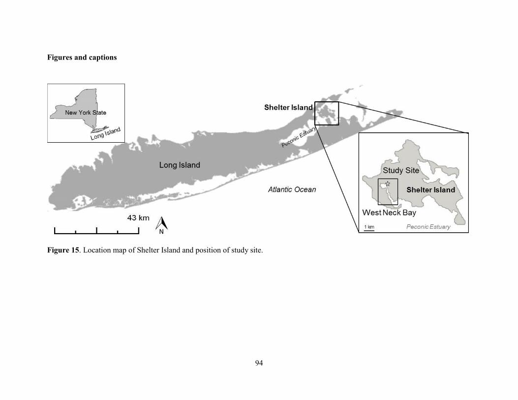
94


Figure 15. Location map of Shelter Island and position of study site.

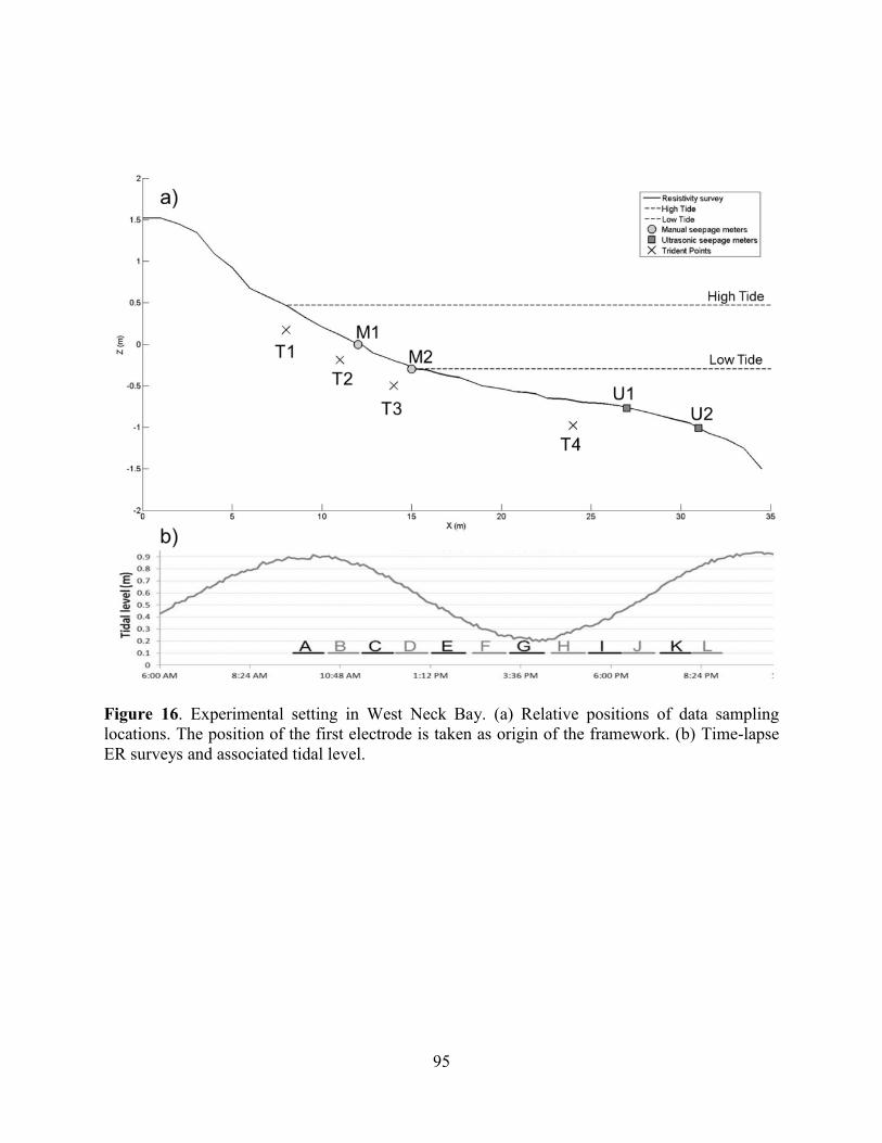
95

Figure 16. Experimental setting in West Neck Bay. (a) Relative positions of data sampling

locations. The position of the first electrode is taken as origin of the framework. (b) Time-lapse

ER surveys and associated tidal level.

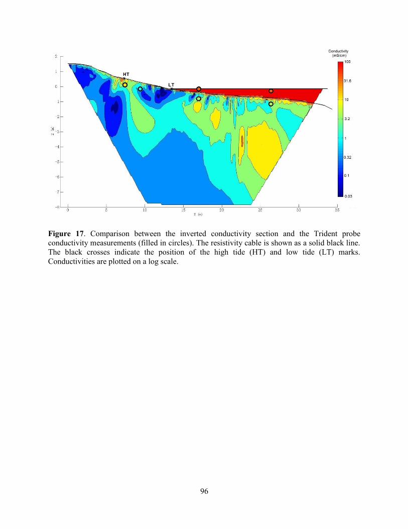
96

Figure 17. Comparison between the inverted conductivity section and the Trident probe

conductivity measurements (filled in circles). The resistivity cable is shown as a solid black line.

The black crosses indicate the position of the high tide (HT) and low tide (LT) marks.

Conductivities are plotted on a log scale.

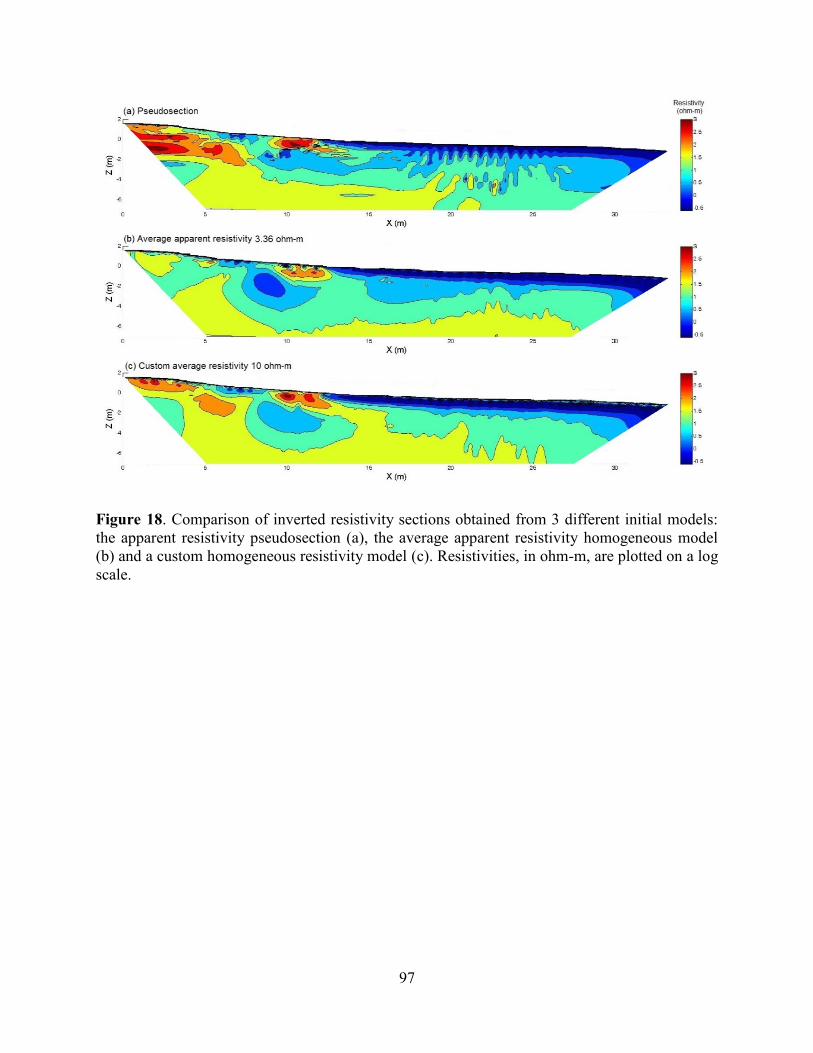
97

Figure 18. Comparison of inverted resistivity sections obtained from 3 different initial models:

the apparent resistivity pseudosection (a), the average apparent resistivity homogeneous model

(b) and a custom homogeneous resistivity model (c). Resistivities, in ohm-m, are plotted on a log

scale.

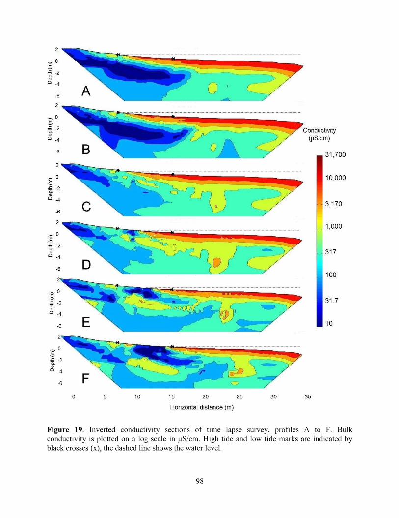
98

Figure 19. Inverted conductivity sections of time lapse survey, profiles A to F. Bulk

conductivity is plotted on a log scale in μS/cm. High tide and low tide marks are indicated by

black crosses (x), the dashed line shows the water level.

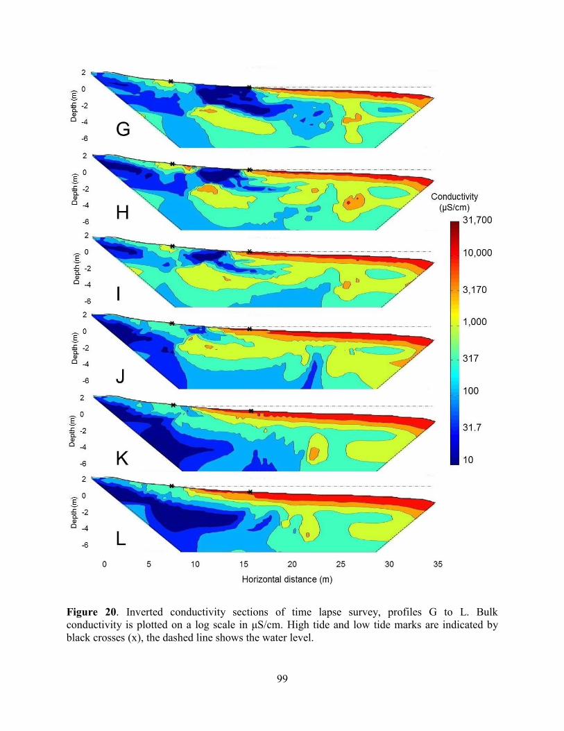
99

Figure 20. Inverted conductivity sections of time lapse survey, profiles G to L. Bulk

conductivity is plotted on a log scale in μS/cm. High tide and low tide marks are indicated by

black crosses (x), the dashed line shows the water level.

100

Figure 21. Average conductivity sections for the high tide (a) and low tide (b) end-members, and

for the phase-averaged profile (c), in μS/cm. Conductivities are plotted on a log scale.

101

Figure 22. Seepage rates and salinity measured with the manual seepage meters M1 (a) and M2

(b) in the intertidal zone.

102

Figure 23. Salinities and freshwater content (%) measured in the manual seepage collection bags (a) and computed for SGD entering

the seepage meters (b).

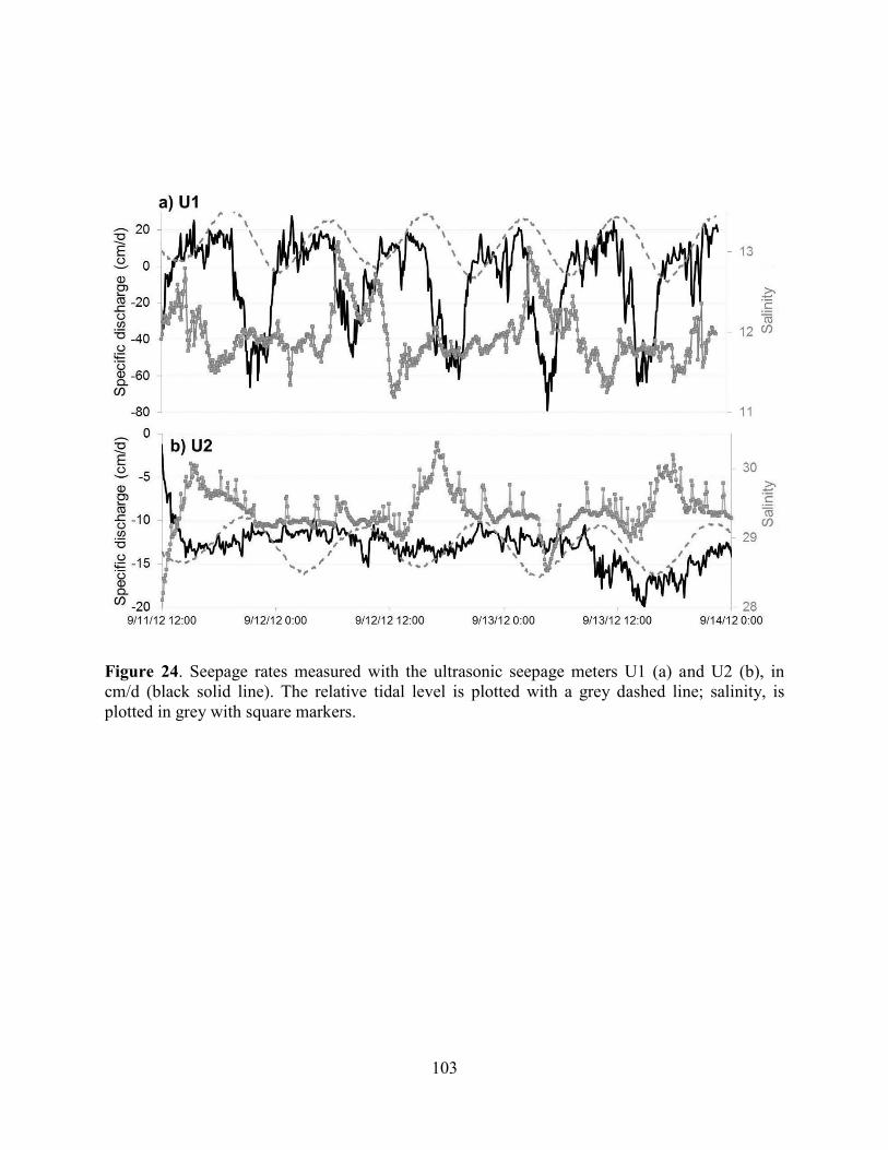
103

Figure 24. Seepage rates measured with the ultrasonic seepage meters U1 (a) and U2 (b), in

cm/d (black solid line). The relative tidal level is plotted with a grey dashed line; salinity, is

plotted in grey with square markers.

104

Chapter 5: Nutrient loading associated with submarine groundwater discharge in Forge

River

Abstract

Forge River, a tidal river located on the south shore of Long Island, has experienced chronic

hypoxia due to excessive nitrogen input for almost a decade. A significant portion of nitrogen is

entering the river through submarine groundwater discharge (SGD). Management and ecological

restoration of the Forge River watershed hinge upon a comprehensive understanding of where

and how nutrient loading is occurring. An integrated approach combining electrical resistivity

surveys, conductivity/temperature and seepage point measurements, and pore water analysis was

used to map out SGD distribution and provide water quality data. We found that nitrogen

speciation and concentration are linked to different SGD regimes distributed in 3 main zones.

The first zone is composed of near shore sandy areas with high SGD. They present little nitrate

reduction and constitute the major source of nitrogen input to surface waters. The second zone

encompasses offshore areas rich in silt and organic matter. They exhibit low SGD and higher

denitrification. Finally, in zone 3, dredging activities have altered the sediment distribution and

subsequently created preferential flow paths focusing freshwater discharge in the center of the

river.

105

1. Introduction

1.1 Background

The Forge River is located between the hamlets of Mastic and Moriches, in southern

Suffolk County, NY (Figure 25). A major tributary of Moriches Bay on the south shore of Long

Island, Forge River has played an important role in producing natural resources for both

commercial and recreational users for many decades. For several decades it has experienced

chronic hypoxia due to excessive nitrogen input from a number of natural and anthropogenic

sources, including submarine discharge that contains effluent from unsewered high-density

residential housing and wastewater from a commercial duck farm upstream. An alarming fish-

kill occurred in the summer of 2006, which increased the concern about a general decline in its

state of health and, consequently, Forge River was added to the 2006 New York State 303(d) List

of Impaired Water Bodies. To date many surface waters along the south shore and east end of

Long Island have areas of severe eutrophication and harmful algal blooms [Burson et al., 2008;

Laroche et al., 1997; Ryther, 1954]. Although recent improvement has been observed in the river

due to closure of the upriver duck farms and recent dredging, concern remains that excessive

nitrogen is entering the river.

Management and ecological restoration of the Forge River watershed hinge upon a

comprehensive understanding of where and how nutrient loading is occurring. As is typical of

Long Island streams, a significant portion of the freshwater flow of Forge River derives from

groundwater, which may transport nutrients from the underground aquifer by submarine

groundwater discharge (SGD). Since this SGD can transport nutrients and contaminants from

inland sources, it plays a key role in controlling the water quality of the surface waters with

significant impact on the ecological condition in these waters [Johannes, 1980; Zektser et al.,

2006]. A recent study of the benthic fluxes of Forge River observed that the flux related to

groundwater is relatively high, representing up to 73% of the total external supply of nitrogen

[Aller, 2009]. As this flux is largest on the more densely populated western side of the Forge

watershed, it has probably contributed to the greater hypoxia and nitrogen, as well as lower

oxygen levels observed in the tributaries and shorelines along this portion of the Forge River.

106

1.2 Objective of the project

By its very nature, the mixing zone between Forge River and Moriches Bay is a dynamic

system that evolves with the interaction between bay water from tidal loading and fresh surface

water, which may involve significant spatial and temporal complexity.

An integrated study was designed to map out areas of pronounced SGD and acquire water

quality data within these zones. I adopted the methodology and protocol that were established by

Paulsen et al. [2008] in the Coastal Contaminant Migration Monitoring Assessment of Forge

River, which integrated the ultrasonic seepage meter with the Trident Probe, a screening probe

that uses electrical conductivity and temperature sensors for mapping out the extent of

groundwater seepage, and the SuperSting, a geophysical tool for mapping out the spatial

distribution of electricity resistivity as a proxy for fresh water discharge. Guided by the spatial

extent of SGD that had been inferred from the SuperSting and Trident Probe measurements,

cluster wells were also positioned in transects across the river to provide in situ nitrogen

speciation and concentration measurements in groundwater. Ultrasonic seepage meters were also

used to measure SGD fluxes at key locations.

Results of past studies revealed that significant concentrations of nitrogen were present in

near-shore groundwater discharging into the Forge River, mostly along the western shoreline

[Paulsen et al., 2008; Wanlass, 2009]. Those studies found that high nutrients inputs were

located in the portion of Forge River analyzed in the present report i.e. transects FR2 and FR1, as

shown in Figure 29. Some ammonia was present in the hypoxic levels (DO < 2 mg/L) at

concentrations varying between 0.02 and 2.25 mg/L, indicating a possible conversion of nitrate

into ammonia in oxygen-depleted areas.

The overall objective of this study is to quantify the nitrogen load related to groundwater

influx across the hyporheic zone at two locations on Forge River. These sites were selected

because they have significant groundwater input, according to previous hydrogeological

investigations and interpretation of well data [Paulsen et al., 2008; Wanlass, 2009]. It should be

noted that a third transect was also investigated at Wills Creek (Figure 29), but is not presented

here as the results were similar to the ones obtained at FR1 and FR2 [Durand and Paulsen,

2014].

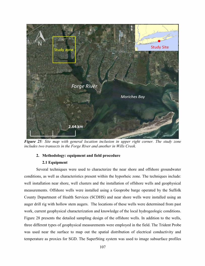
107

Figure 25: Site map with general location inclusion in upper right corner. The study zone

includes two transects in the Forge River and another in Wills Creek.

2. Methodology: equipment and field procedure

2.1 Equipment

Several techniques were used to characterize the near shore and offshore groundwater

conditions, as well as characteristics present within the hyporheic zone. The techniques include:

well installation near shore, well clusters and the installation of offshore wells and geophysical

measurements. Offshore wells were installed using a Geoprobe barge operated by the Suffolk

County Department of Health Services (SCDHS) and near shore wells were installed using an

auger drill rig with hollow stem augers. The locations of these wells were determined from past

work, current geophysical characterization and knowledge of the local hydrogeologic conditions.

Figure 28 presents the detailed sampling design of the offshore wells. In addition to the wells,

three different types of geophysical measurements were employed in the field. The Trident Probe

was used near the surface to map out the spatial distribution of electrical conductivity and

temperature as proxies for SGD. The SuperSting system was used to image subsurface profiles

108

of electrical resistivity along selected vertical sections transverse to the shoreline. The ultrasonic

seepage meter system was deployed at selected locations to quantify SGD.

2.1.1 Trident Probe

The Trident probe is a direct-push instrument developed to screen and assess offshore

areas where groundwater may be discharging to the surface water body [Chadwick et al., 2003].

The probe integrates two temperature sensors, two electrical conductivity sensors, and two pore

water samplers. The subsurface conductivity/temperature (C/T) probe measures the electrical

conductivity and temperature at depth, whereas the surface C/T sensors measure the electrical

conductivity and temperature of the water in the vicinity of the Trident probe. The subsurface

C/T probe and the dual pore water samplers are collocated in a triangular pattern with a spacing

of about 10 cm on an aluminum stopper/sealer plate that rests on the sediment-water interface.

By adjusting the position of the mounting plate relative to the subsurface probes, measurements

can be conducted at different depths. In this study, the depth was typically fixed at 45.7 cm (18”)

below the sediment-water interface.

Each conductivity sensor is made up of two pairs of stainless steel electrodes that make

up a Wenner array. A known current is imposed on the outer pair of electrodes, while the voltage

through the inner pair is monitored. The apparent conductivity of the saturated sediments and its

spatial variation is primarily a function of changes in salinity, and secondarily of clay content

and porosity. In this setting, it is likely that an area with relatively low conductivity is associated

with SGD. The temperature sensor consists of a customized digital oceanographic thermometer

with a ruggedized titanium probe. It has a measurement range of -5 to +35 °C at an accuracy of

0.001 °C, and a resolution of 0.00025 °C. Areas of groundwater seepage may appear either as

warm or cold contrast to the surface water, depending on the seasonal and site characteristics.

Once such a likely area of groundwater impingement has been identified, the dual water-

sampling probes can be used to collect samples for on-site field parameter characterization

(salinity, DO, ORP, pH) and for detailed analysis of chemical constituents by off-site

laboratories. The head of the push-pole of the Trident probe is fitted with a global positioning

system (GPS) unit with wide-area augmentation system (WAAS) capability. Hence the data

logger also captures spatial coordinates of the location where subsurface and surface

measurements of electrical conductivity and temperature are measured.

109

2.1.2 Supersting Resistivity system

Electrical resistivity imaging was performed using the SuperSting R8 system, and the

acquired data were analyzed using the software package EarthImager 2D. The SuperSting system

uses a cable of length 33 m (112’), with 56 electrodes separated by a uniform spacing of 0.61 m

(2’). It is capable of simultaneously measuring 8 channels using a high-power transmitter. The

control box injects current in the cable every 3 seconds, and 8 apparent resistivity values

representing 8 depth levels are read for each current injection. The control box assigns which

electrode shall be the current injector and which shall be the potential reader, in accordance with

the specific array configuration that has been selected. In this study, measurements were made

using both the dipole-dipole and Schlumberger configurations at each site, and the data were

stacked together for the inverse analysis. The dipole-dipole configuration is useful to study

shallow variations; the Schlumberger allows a deeper penetration and a greater lateral resolution.

Using 2-dimensional resistivity inversion, the software package EarthImager2D interprets

the apparent resistivity data acquired by the SuperSting array and provides optimal estimation of

the spatial distribution of resistivity on the vertical profile. In this study the software has been

implemented following the procedure described by [Durand et al., 2011].

2.1.3 Ultrasonic seepage meter

SGD was quantified using an ultrasonic seepage meter developed by [Paulsen et al.,

2001]. SGD is captured by a steel collection chamber (with a diameter of 45.72 cm (18”) and a

round cross section of 0.164 m2), inserted approximately 10 cm into the sediment. The discharge

so captured is directed to a cylindrical flow tube with two piezoelectric transducers mounted at

opposite ends. The transducers continually generate bursts of ultrasonic signals (periodic waves

with a frequency of 1.7 MHz) from one end of the meter to the other end, while arrival of the

ultrasonic signals is continuously monitored by the piezoelectric transducers. If velocity of the

flow induced by the SGD in the tube is small relative to the ambient sound velocity and if the

fluctuations of temperature and salinity are negligible, then the flow velocity is directly

proportional to the difference between the upstream and downstream arrival times. Taking into

account the areal ratio between flow tube and collection chamber, the specific discharge of the

submarine ground water can be calculated from the flow velocity in the tube. The meter is

capable of continuously measuring SGD at rates as low as 0.07 m/s (0.25 cm/d). In parallel,

110

the water temperature and conductivity are collected using a solinst level logger attached to the

underside of the seepage funnel. The sampling rate is 10 seconds and is used to determine the

specific discharge.

The ultrasonic groundwater seepage meter was deployed following the protocol described in

[Chadwick et al., 2003; Chadwick et al., 2003]. Data calibration for the ultrasonic seepage meter

requires to record null fluxes before and after each deployment and are called prezero and

postzero. The prezero and postzero allow checking the stability of the meter during deployment,

their average is deducted from the discharge measured in the field to remove the error created by

the seepage meter itself.

2.2 Field procedure

2.2.1 Trident probe

In some cases, the lithology and geological conditions were such that the subsurface

probes of the Trident met with significant resistance at a depth less than the target depth of 45.7

cm, which required relocating the sampling point by a lateral distance of approximately 30-60

cm for another trial to penetrate the probes down to the target depth. Occasionally it was

necessary to repeat the process up to three times before a successful installation was

accomplished. In sediments that were silty, it was sometimes difficult to extract water samples.

The locations of Trident stations were chosen according to knowledge of the site acquired from

previous studies. Pore water was pumped using the water-sampling probe powered by a low-flow

peristaltic pumping system, for nutrients analyses. Prior to sampling, the system was purged by

first pumping and discharging approximately 60 ml (3 sampler volumes using a 10 m sample

tube). Conductivity and temperature of collected pore water were simultaneously measured using

a YSI multimeter probe. Readings were monitored until they were stable, then logged over a

sixty second interval and averaged by the recording software. Records also include the time, date

and location of the station. After the station was logged, samples were collected for water quality

measurements using the YSI 556 hand-held probe for temperature, conductivity, salinity,

dissolved oxygen, pH and oxydo-reduction potential (ORP).

Samples for phosphate analysis were collected in 250 ml amber glass bottles. Samples for

standard inorganic analysis (nitrogen series, phosphate and silica) were collected in HDPE, 250

ml screw cap bottles. Between points, the screen zone was disassembled, brushed to remove

111

attached sediments, rinsed with seawater and deionized water (DI) and put back in place. The

entire sampling system was flushed with a series of solutions including: a 1/10 alcanox aqueous

solution, surface water, and DI water. All samples were unfiltered. Care was taken during the

pumping process to minimize the amount of suspended solids in the samples.

Figure 26: Site map showing Trident point locations associated with the wells, in Wills Creek

and Forge River.

Trident transect were acquired at three locations: FR1, FR2 and WC between 6/19/13 and

7/9/13 to explore the shallow pore water temperature and conductivity distribution (Figure 26).

Two tables summarizing the Trident records are available in appendix (Appendix 1 and

Appendix 2).

2.2.2 Supersting resistivity and EarthImager2D

The SuperSting cable was deployed on the sediment bottom along transects running

perpendicular to the shoreline, north/south for Wills Creek and west/east for Forge River. If part

of the cable was exposed, additional electrode spikes were added and coupled to the cable to

ensure proper contact with the ground. All resistivity surveys were acquired at low tide. At two

transect locations on FR1 and FR2 a high tide measurement of resistivity was performed in order

to capture tidal variability. To limit the variations of the overlying surface water layer during a

112

given resistivity survey, the acquisition was scheduled so that the minimum or maximum tidal

stage would occur at the middle of the data acquisition period.

Bathymetry profiles and muck layer profiles were always performed simultaneously to

the electrical resistivity surveys. Trident points were associated with ER measurements for

ground-truthing. The positions of the electrical resistivity surveys for Forge River are shown in

Figure 27. The offset observed between the transects FR1A, FR1B and the wells results from

various difficulties encountered in the field. Due to some problems with the SuperSting, the

acquisition of electrical resistivity transects had to be repeated several times at different location

before obtaining satisfying results. Anchoring the boat was also challenging in this area, so it

was not possible to position it as accurately as for the other sites. Finally, malfunction of the GPS

forced us to use a different unit with slightly different accuracy.

2.2.3 Ultrasonic seepage meter

Guided by the other measurements on the spatial distribution of SGD, two locations along

the transect FR2 were selected for deployment of the ultrasonic seepage meters in Forge River:

close to the shore and in the middle of the river. The seepage meters were left in place for a

period of two days on July 24th

and 25th

, 2013. Technical difficulties only allowed us to obtain

data from the location closest to the shore (Figure 27). For both the ultrasonic seepage meter

deployment and the electrical resistivity measurements a Solinst pressure logger was deployed at

the marina to monitor the tidal level. By plotting the measured tidal variation along with the

predicted tides given by the MapTech ProChart Navigation software, we observed that the tidal

variations in the creek and the river have about 65 % the amplitude of the predictions at the

Moriches Coast Gard Station and a lag of ~1h. Solinst multiloggers were deployed in the funnels

to record pressure, temperature and conductivity of seepage but technical problems (erratic

readings by logger or incomplete record) did not allow recovering the data. The software

predictions were then corrected and used as tidal level indicator.

113

Figure 27: Site map of electrical resistivity surveys and well profiles at FR1 and FR2 and

ultrasonic seepage meter location, in Forge River.

2.2.4 Water sampling

2.2.4.1 Well design

The sampling design of the offshore sediment bottom included 5 sample points at depth

along five stations transecting the river at three locations. Typically, there is a muck/silt layer

overlying a layer of sand and gravel (Figure 28). The upper pore fluids were collected using

temporary Trident Probe at two points located at 0.3 to 0.7 m (1 to 2 ft) bellow the

sediment/water interface. The third temporary point was set at the interface between the

underlying sandy bottom and the silt/muck layer. Typically the sample point was set 0.3 m (1 ft)

into the sandy bottom. The deeper pore fluids were collected using offshore semi-permanent one

inch piezometers. The 4th

and 5th

points were set at 3 and 6 m (10 and 20 ft) below the

sandy/muck interface. Figure 28 provides the conceptual sampling design. Although slightly

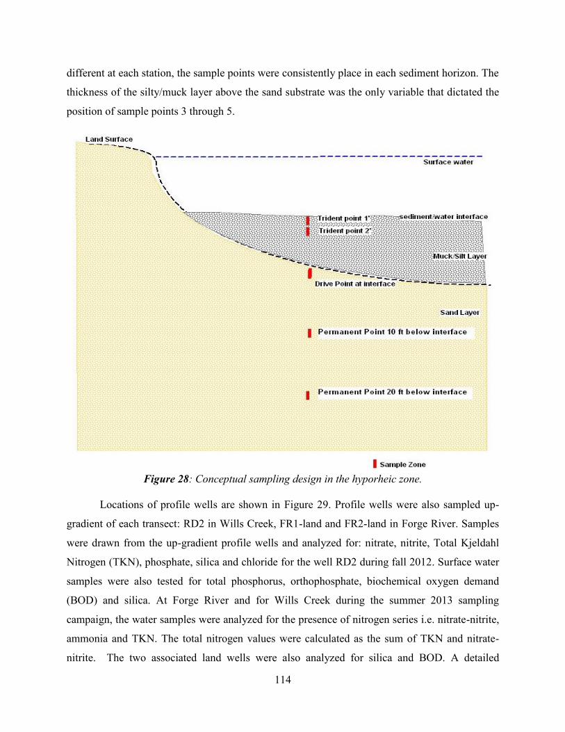
114

different at each station, the sample points were consistently place in each sediment horizon. The

thickness of the silty/muck layer above the sand substrate was the only variable that dictated the

position of sample points 3 through 5.

Figure 28: Conceptual sampling design in the hyporheic zone.

Locations of profile wells are shown in Figure 29. Profile wells were also sampled up-

gradient of each transect: RD2 in Wills Creek, FR1-land and FR2-land in Forge River. Samples

were drawn from the up-gradient profile wells and analyzed for: nitrate, nitrite, Total Kjeldahl

Nitrogen (TKN), phosphate, silica and chloride for the well RD2 during fall 2012. Surface water

samples were also tested for total phosphorus, orthophosphate, biochemical oxygen demand

(BOD) and silica. At Forge River and for Wills Creek during the summer 2013 sampling

campaign, the water samples were analyzed for the presence of nitrogen series i.e. nitrate-nitrite,

ammonia and TKN. The total nitrogen values were calculated as the sum of TKN and nitrate-

nitrite. The two associated land wells were also analyzed for silica and BOD. A detailed

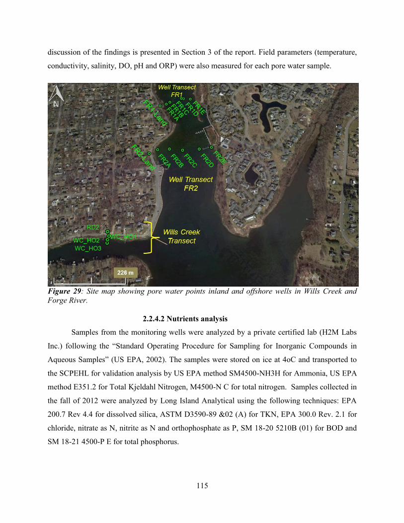
115

discussion of the findings is presented in Section 3 of the report. Field parameters (temperature,

conductivity, salinity, DO, pH and ORP) were also measured for each pore water sample.

Figure 29: Site map showing pore water points inland and offshore wells in Wills Creek and

Forge River.

2.2.4.2 Nutrients analysis

Samples from the monitoring wells were analyzed by a private certified lab (H2M Labs

Inc.) following the “Standard Operating Procedure for Sampling for Inorganic Compounds in

Aqueous Samples” (US EPA, 2002). The samples were stored on ice at 4oC and transported to

the SCPEHL for validation analysis by US EPA method SM4500-NH3H for Ammonia, US EPA

method E351.2 for Total Kjeldahl Nitrogen, M4500-N C for total nitrogen. Samples collected in

the fall of 2012 were analyzed by Long Island Analytical using the following techniques: EPA

200.7 Rev 4.4 for dissolved silica, ASTM D3590-89 &02 (A) for TKN, EPA 300.0 Rev. 2.1 for

chloride, nitrate as N, nitrite as N and orthophosphate as P, SM 18-20 5210B (01) for BOD and

SM 18-21 4500-P E for total phosphorus.

116

2.2.4.3 In situ pore water analysis

Samples obtained from the Trident and from the wells were analyzed on-site using a YSI

556 hand-held multi probe. The YSI probe detects temperature, conductivity, salinity, pH, DO

and ORP. The YSI probe was calibrated to specific conductivity standards prior to the beginning

of each survey. In addition, the Trident system measured temperature and conductance in the

sediment bottom.

3. Results

3.1 Trident mapping and pore water conductivity sections

Electrical conductivity and temperature data from the Trident surveys associated with the

offshore wells are presented in Appendix 2. As noted earlier, the data were typically acquired at

a fixed depth of 45.7 cm (18”) below the sediment-water interface. The subsurface C/T probe

measures the electrical conductivity and temperature of the saturated sediment at depth, whereas

the surface C/T sensors measure the reference electrical conductivity and temperature of the

surface water in the vicinity of the Trident probe. The properties measured with the C/T probe in

the shallow sediments depend on both porous medium and the saturating fluid properties.

The results from the Trident point transects associated with the well sampling at Forge

River are presented in Figure 30. The difference in surface water temperature between FR1 and

FR2 is the results of different acquisition weeks (Figure 30a). Bulk temperatures and

conductivities for transect FR1 vary slightly around 20°C and 8 mS/cm, respectively, indicating

some mixing between fresh groundwater and surface water. Surface water conductivities are

lower close to both shores and in the center of the river, revealing freshwater discharge (Figure

30d). The conductivity difference, defined as ∆C = Cporewater – Csurface water, is smaller close the

shores indicating some limited mixing with the surface water. The analysis of FR2 is slightly

different. The bulk conductivity distribution is more homogeneous and all the values are very

low < 5 mS/cm which reveals the presence of fresh groundwater, isolated under the muck layer,

across the whole river. A relatively low value of surface water conductivity, 25 mS/cm, close to

the east shore, indicates significant freshwater discharge in the area. Previous studies had found

that seepage was found mostly on the west shore [Wanlass, 2009], but our data suggest that the

discharge on the east shore is not negligible.

117

Points at the center of the river in transects FR1 and FR2 stand out from the other

sampling points: they have low bulk and surface water conductivities, i.e. < 5 mS/cm and < 10

mS/cm, respectively (Figure 30c), which results in very small conductivity and temperature

differences (Figure 30e). This indicates that the reference probe (or surface water probe), located

a few inches above the probe inserted into the sediments, is sampling seeping groundwater fluid

that has not been mixed with the overlying surface water. Two scenarios can explain the low

conductivities of the overlying water at the center of the river: a strong fresh SGD flux or a

misplacement of the reference probe inside the muck layer, enabled by the fluidity of that layer.

High SGD rates are unexpected in areas where the low permeability muck layer is at least 1.5 m

(5 ft) thick.

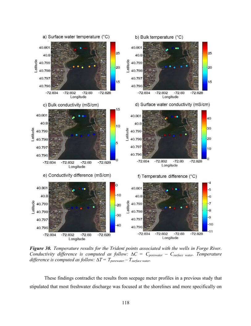
118

Figure 30. Temperature results for the Trident points associated with the wells in Forge River.

Conductivity difference is computed as follow: ∆C = Cporewater – Csurface water. Temperature

difference is computed as follow: ∆T = Tporewater – Tsurface water.

These findings contradict the results from seepage meter profiles in a previous study that

stipulated that most freshwater discharge was focused at the shorelines and more specifically on

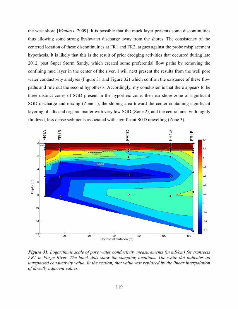
119

the west shore [Wanlass, 2009]. It is possible that the muck layer presents some discontinuities

thus allowing some strong freshwater discharge away from the shores. The consistency of the

centered location of these discontinuities at FR1 and FR2, argues against the probe misplacement

hypothesis. It is likely that this is the result of prior dredging activities that occurred during late

2012, post Super Storm Sandy, which created some preferential flow paths by removing the

confining mud layer in the center of the river. I will next present the results from the well pore

water conductivity analyses (Figure 31 and Figure 32) which confirm the existence of these flow

paths and rule out the second hypothesis. Accordingly, my conclusion is that there appears to be

three distinct zones of SGD present in the hyporheic zone: the near shore zone of significant

SGD discharge and mixing (Zone 1), the sloping area toward the center containing significant

layering of silts and organic matter with very low SGD (Zone 2), and the central area with highly

fluidized, less dense sediments associated with significant SGD upwelling (Zone 3).

Figure 31. Logarithmic scale of pore water conductivity measurements (in mS/cm) for transects

FR1 in Forge River. The black dots show the sampling locations. The white dot indicates an

unreported conductivity value. In the section, that value was replaced by the linear interpolation

of directly adjacent values.

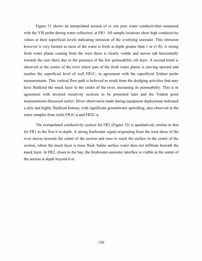
120

Figure 31 shows an interpolated section of in situ pore water conductivities measured

with the YSI probe during water collection, at FR1. All sample locations show high conductivity

values at their superficial levels indicating intrusion of the overlying seawater. This intrusion

however is very limited as most of the water is fresh at depth greater than 1 m (3 ft). A strong

fresh water plume coming from the west shore is clearly visible and moves sub horizontally

towards the east shore due to the presence of the low permeability silt layer. A second trend is

observed in the center of the river where part of the fresh water plume is moving upward and

reaches the superficial level of well FR1C, in agreement with the superficial Trident probe

measurements. This vertical flow path is believed to result from the dredging activities that may

have fluidized the muck layer in the center of the river, increasing its permeability. This is in

agreement with inverted resistivity sections to be presented later and the Trident point

measurements discussed earlier. Diver observation made during equipment deployment indicated

a silty and highly fluidized bottom, with significant groundwater upwelling, also observed in the

water samples from wells FR1C-a and FR2C-a.

The extrapolated conductivity section for FR2 (Figure 32) is qualitatively similar to that

for FR1 in the first 6 m depth. A strong freshwater signal originating from the west shore of the

river moves towards the center of the section and rises to reach the surface in the center of the

section, where the muck layer is more fluid. Saline surface water does not infiltrate beneath the

muck layer. In FR2, closer to the bay, the freshwater-seawater interface is visible in the center of

the section at depth beyond 6 m.

121

Figure 32. Logarithmic scale of conductivity measurements (in mS/cm) for transect FR2 in

Forge River. The black dots show the sampling locations.

3.2 Electrical resistivity surveys

The inverted conductivity sections for transect FR1, located in the upper section of the

Forge river, show that there is a diffuse zone of very low conductivity (between 0.04 and 0.5

mS/cm), that reveals the presence of fresh water (Figure 33). The freshwater signal is stronger on

the west shore of Forge River. The plume extends under most of this river section, likely due to

the hydraulic confinement exerted by the low-permeability muck layer, also present in most of

this section. Two significant areas of fresh groundwater are detected around x ~ 28 m and x ~ 55

m offshore and extend down to a depth of 10 m.

The inverted conductivity sections for transect FR2 is quantitatively similar. There is a

diffuse zone of very low conductivity (between 0.04 and 0.5 mS/cm) (Figure 34, Figure 35 and

Figure 36). The freshwater signal is stronger on the west shore of Forge River but a significant

amount of freshwater is present in the middle area at various locations. The freshwater cell also

extends under most of this river section, likely due to the hydraulic confinement by the muck

layer. Two areas of fresh groundwater were detected at ~ 35 and 60 m offshore (measured from

122

western shoreline) and extended down to a depth of 16 m. A third area with freshwater is visible

at x ~ 30 m offshore of the eastern shoreline.

Figure 33: Inverted conductivity sections of profile FR1A and FR1B at the west and east shore

of Forge River, respectively.

The survey FR2A was repeated at low and high tide to study the tidal influence on the

freshwater distribution (Figure 34). The two surveys are consistent, and there is not much

difference in the horizontal extent of the freshwater plume. However, the freshwater plume

seems to be focused closer to the shore at high tide and farther offshore at low tide. Given the

limited influence of tidal variations on the resistivity profiles, surveys FR2B and FR2C were

only acquired at low tide.

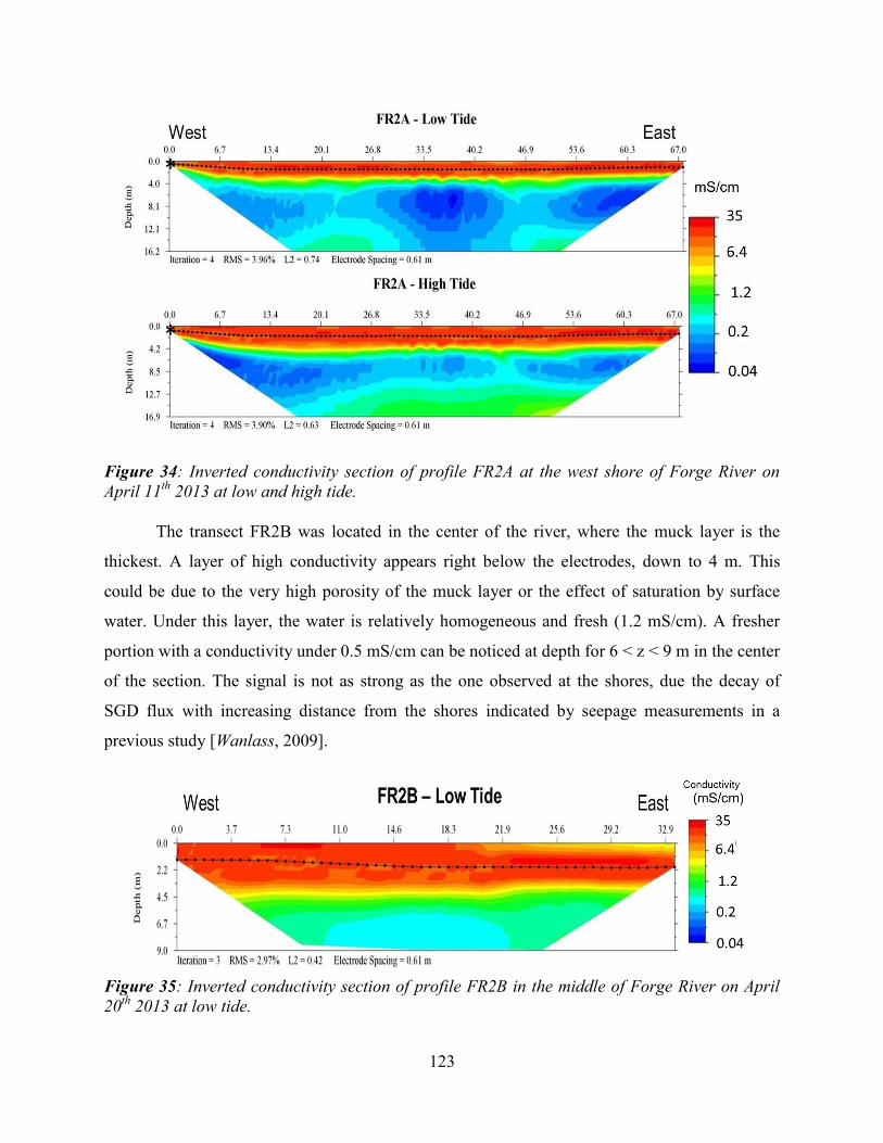
123

Figure 34: Inverted conductivity section of profile FR2A at the west shore of Forge River on

April 11th

2013 at low and high tide.

The transect FR2B was located in the center of the river, where the muck layer is the

thickest. A layer of high conductivity appears right below the electrodes, down to 4 m. This

could be due to the very high porosity of the muck layer or the effect of saturation by surface

water. Under this layer, the water is relatively homogeneous and fresh (1.2 mS/cm). A fresher

portion with a conductivity under 0.5 mS/cm can be noticed at depth for 6 < z < 9 m in the center

of the section. The signal is not as strong as the one observed at the shores, due the decay of

SGD flux with increasing distance from the shores indicated by seepage measurements in a

previous study [Wanlass, 2009].

Figure 35: Inverted conductivity section of profile FR2B in the middle of Forge River on April

20th

2013 at low tide.

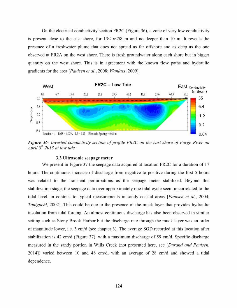
124

On the electrical conductivity section FR2C (Figure 36), a zone of very low conductivity

is present close to the east shore, for 13< x<58 m and no deeper than 10 m. It reveals the

presence of a freshwater plume that does not spread as far offshore and as deep as the one

observed at FR2A on the west shore. There is fresh groundwater along each shore but in bigger

quantity on the west shore. This is in agreement with the known flow paths and hydraulic

gradients for the area [Paulsen et al., 2008; Wanlass, 2009].

Figure 36: Inverted conductivity section of profile FR2C on the east shore of Forge River on

April 8th

2013 at low tide.

3.3 Ultrasonic seepage meter

We present in Figure 37 the seepage data acquired at location FR2C for a duration of 17

hours. The continuous increase of discharge from negative to positive during the first 5 hours

was related to the transient perturbations as the seepage meter stabilized. Beyond this

stabilization stage, the seepage data over approximately one tidal cycle seem uncorrelated to the

tidal level, in contrast to typical measurements in sandy coastal areas [Paulsen et al., 2004;

Taniguchi, 2002]. This could be due to the presence of the muck layer that provides hydraulic

insolation from tidal forcing. An almost continuous discharge has also been observed in similar

setting such as Stony Brook Harbor but the discharge rate through the muck layer was an order

of magnitude lower, i.e. 3 cm/d (see chapter 3). The average SGD recorded at this location after

stabilization is 42 cm/d (Figure 37), with a maximum discharge of 59 cm/d. Specific discharge

measured in the sandy portion in Wills Creek (not presented here, see [Durand and Paulsen,

2014]) varied between 10 and 48 cm/d, with an average of 28 cm/d and showed a tidal

dependence.

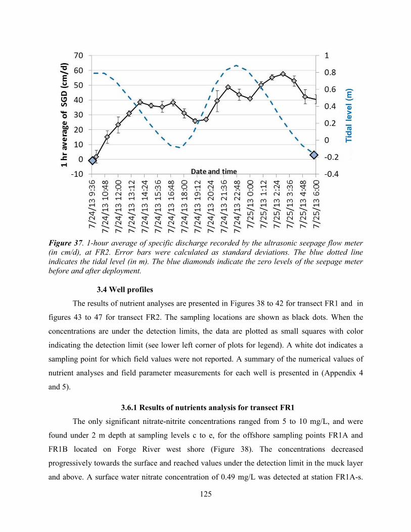
125

Figure 37. 1-hour average of specific discharge recorded by the ultrasonic seepage flow meter

(in cm/d), at FR2. Error bars were calculated as standard deviations. The blue dotted line

indicates the tidal level (in m). The blue diamonds indicate the zero levels of the seepage meter

before and after deployment.

3.4 Well profiles

The results of nutrient analyses are presented in Figures 38 to 42 for transect FR1 and in

figures 43 to 47 for transect FR2. The sampling locations are shown as black dots. When the

concentrations are under the detection limits, the data are plotted as small squares with color

indicating the detection limit (see lower left corner of plots for legend). A white dot indicates a

sampling point for which field values were not reported. A summary of the numerical values of

nutrient analyses and field parameter measurements for each well is presented in (Appendix 4

and 5).

3.6.1 Results of nutrients analysis for transect FR1

The only significant nitrate-nitrite concentrations ranged from 5 to 10 mg/L, and were

found under 2 m depth at sampling levels c to e, for the offshore sampling points FR1A and

FR1B located on Forge River west shore (Figure 38). The concentrations decreased

progressively towards the surface and reached values under the detection limit in the muck layer

and above. A surface water nitrate concentration of 0.49 mg/L was detected at station FR1A-s.

126

No nitrates were found in the surface water at other surface water stations. All values from the

center of the river to the east shore were low, under 2 mg/L. The nitrate plume was localized to

the western shore of Forge River.

Denitrification is defined as the reduction of nitrate by heterotrophic organisms leading to

the production of molecular nitrogen (N2(g)) through a series of intermediate gaseous nitrogen

oxide products [Zumft, 1997]. These microorganisms use nitrate when the concentration of

oxygen is low enough (under 2mg/L), and also require organic carbon as a source for energy.

A number of microorganisms reduce nitrate to ammonia which is assimilated as a source

of nitrogen for biosynthesis [Payne, 1973]. Several heterotrophic bacteria (E. coli, Azospirillum)

are capable of converting nitrates to nitrites and nitrites to ammonia. This process called

ammonification is associated with sediments containing a high organic content, such as those in

the Forge River. It has been suggested that the pathway of nitrate reduction to ammonia is

important in coastal sediments [Koike and Hattori, 1978]. Nitrate reduction normally occurs

under anaerobic soil conditions (water logged soils). This process is not considered to be the

major denitrification process in the Forge but may be a secondary process and explains elevated

concentrations of ammonia in areas where significant organic nitrogen was present. Dissolved

organic nitrogen can form inside the microbial cells and may be excreted and/or liberated from

the cells after their death [Koike and Hattori, 1978].

The ammonia distribution was also very localized, and limited to the muck layer (Figure

39). Relatively high values were found in the two upper levels of wells FR1A, B and D, where

concentrations varied between 10 to 18 mg/L. The rest of the section exhibits very low ammonia

concentrations, typically under 2 mg/L. The high incidence of ammonia in the muck layer,

coincides with low nitrate values, and suggests potential ammonification of nitrogen (organic or

nitrate) by microbial organisms. This is also consistent with the dissolved oxygen section (Figure

42) showing that the high values of ammonia match low levels of dissolved oxygen, under 2-3

mg/L, since oxygen would prevent denitrification as nitrate is a less favorable electron acceptor.

It is likely that the microbial activity is enhanced in the muck layer as the organic matter

provides energy to the microorganisms [Koike and Hattori, 1978].

127

Total Kjeldahl Nitrogen (TKN) is defined as the sum of organic nitrogen, ammonia

(NH3) and ammonium (NH4+). The total nitrogen concentrations are not measured by the

laboratory but calculated as the sum of TKN and nitrate-nitrite values (Figure 41). The results

show that the TKN concentrations match the distribution of ammonia (Figure 40). However, it is

possible to calculate the amount of organic nitrogen and ammonium by subtracting the

concentrations of ammonia from TKN. For most locations, the values of organic nitrogen are

very low and vary between 0 – 2 mg/L but in some locations (well FR1A upper level and FR1C

limit of muck layer) the amount of organic nitrogen reaches 6 – 8 mg/L. This argues in favor of

ammonification of nitrates by microbes, as dissolved organic nitrogen can form inside the

microbial cells and may be excreted and/or liberated from the cells after their death [Koike and

Hattori, 1978].

Figure 38: Nitrate-Nitrite concentrations (in mg/L) from transect FR1 in Forge River.

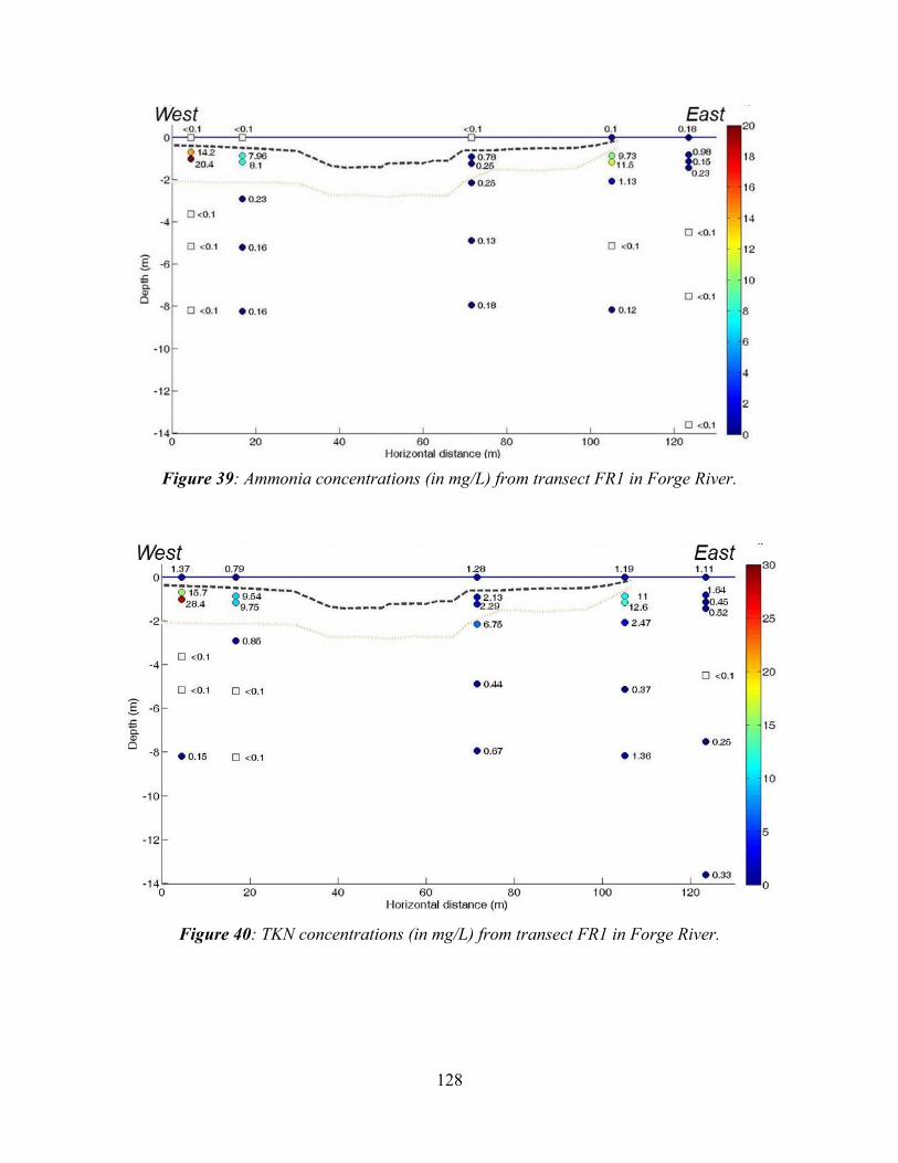
128

Figure 39: Ammonia concentrations (in mg/L) from transect FR1 in Forge River.

Figure 40: TKN concentrations (in mg/L) from transect FR1 in Forge River.

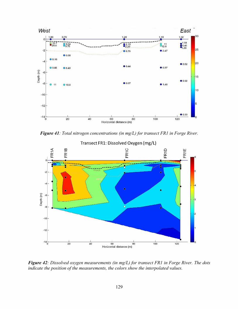
129

Figure 41: Total nitrogen concentrations (in mg/L) for transect FR1 in Forge River.

Figure 42: Dissolved oxygen measurements (in mg/L) for transect FR1 in Forge River. The dots

indicate the position of the measurements, the colors show the interpolated values.

130

The dissolved oxygen concentrations are strongly zoned across the river (Figure 42).

Surface waters and the west portion of the section are rich in oxygen. For the rest of the section,

from the center of the river to the east shore and a shallow level of well FR1A in the muck layer,

the groundwater is depleted in oxygen. The low levels of oxygen observed in the vicinity of the

muck layer, at FR1A-a and FR1D-b, coincide with the high level of ammonia and delineate

where denitrification is possible and/or the production of ammonia from organic matter rich

muck layer.

In conclusion, it appears that the hyporheic zone is divided into three zones with distinct

SGD characteristics and nutrient fluxes, as described in section 3.1.4. The near shore zone 1 (~10

m) has significant advective flows and is an area where denitrification and mixing are likely

occurring. The evidence for this is the decreasing values of nitrates coming from inland

groundwater that are not present in upper section of this zone as wells as the low DO in these

sediments. Looking solely at the water quality results at each station in zone 1, there is evidence

that nitrogen is being reduced in this zone, ranging of 0 to 25%. Based on station FR2A levels e

through b we see a 24.5% reduction in nitrate concentration within the zone, but compared to the

inland well data, there appears to be evidence of further reduction. Since the flow paths and time

of sampling may not coincide, it is hard to verify further reduction. In general the groundwater

near shore has consistently shown nitrogen concentrations in the 5 to 10+ mg/L range.

Considering only the samples within zone we present the reduction of nitrates to be ranging from

0 to 25%.This zone, however, is also a mixing zone when surface water infiltrates the sediments

during high tides. Ammonia and organic nitrogen are present in the zone, likely due to organic

matter mixing and/or microbial activity in the sandy sediments. Ammonia production is likely in

areas with organic nitrogen and low DO, these conditions are present in this area. The area

immediately offshore (10 to 90 m) is characteristic of zone 2 with significant layer of organic

rich sediments (muck layer) and little SGD present. The area has lower concentration of total

nitrogen than near shore sediments and has little nitrogen at depth, which suggests denitrification

occurring and/or mixing of groundwater flow paths. The low DO concentration supports this.

The flux of nitrogen to the river is likely benthic flux in organic forms. A similar zone is present

along in the near shore area along the eastern shoreline (~10 to 20 m offshore). The third area (90

to 110 m) has the characteristic of zone 3 in that the presence of SGD is significant at the

sediment surface and sediments are highly fluidized. The concentrations of total nitrogen are low

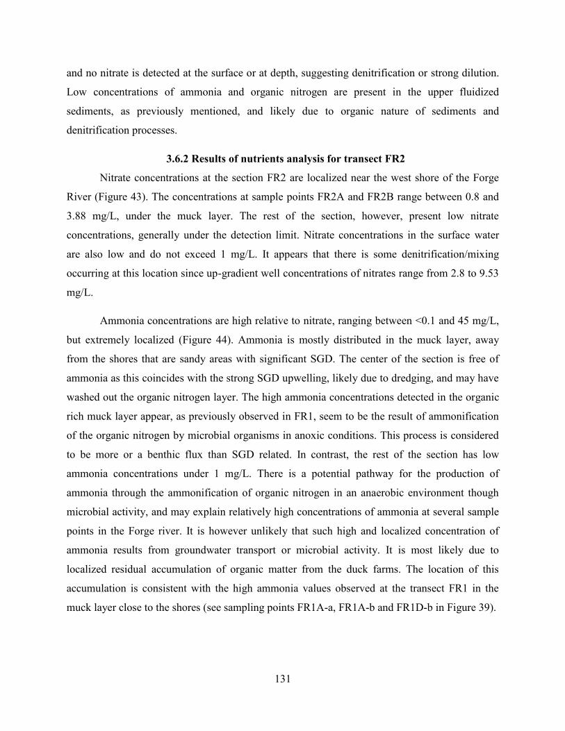
131

and no nitrate is detected at the surface or at depth, suggesting denitrification or strong dilution.

Low concentrations of ammonia and organic nitrogen are present in the upper fluidized

sediments, as previously mentioned, and likely due to organic nature of sediments and

denitrification processes.

3.6.2 Results of nutrients analysis for transect FR2

Nitrate concentrations at the section FR2 are localized near the west shore of the Forge

River (Figure 43). The concentrations at sample points FR2A and FR2B range between 0.8 and

3.88 mg/L, under the muck layer. The rest of the section, however, present low nitrate

concentrations, generally under the detection limit. Nitrate concentrations in the surface water

are also low and do not exceed 1 mg/L. It appears that there is some denitrification/mixing

occurring at this location since up-gradient well concentrations of nitrates range from 2.8 to 9.53

mg/L.

Ammonia concentrations are high relative to nitrate, ranging between <0.1 and 45 mg/L,

but extremely localized (Figure 44). Ammonia is mostly distributed in the muck layer, away

from the shores that are sandy areas with significant SGD. The center of the section is free of

ammonia as this coincides with the strong SGD upwelling, likely due to dredging, and may have

washed out the organic nitrogen layer. The high ammonia concentrations detected in the organic

rich muck layer appear, as previously observed in FR1, seem to be the result of ammonification

of the organic nitrogen by microbial organisms in anoxic conditions. This process is considered

to be more or a benthic flux than SGD related. In contrast, the rest of the section has low

ammonia concentrations under 1 mg/L. There is a potential pathway for the production of

ammonia through the ammonification of organic nitrogen in an anaerobic environment though

microbial activity, and may explain relatively high concentrations of ammonia at several sample

points in the Forge river. It is however unlikely that such high and localized concentration of

ammonia results from groundwater transport or microbial activity. It is most likely due to

localized residual accumulation of organic matter from the duck farms. The location of this

accumulation is consistent with the high ammonia values observed at the transect FR1 in the

muck layer close to the shores (see sampling points FR1A-a, FR1A-b and FR1D-b in Figure 39).

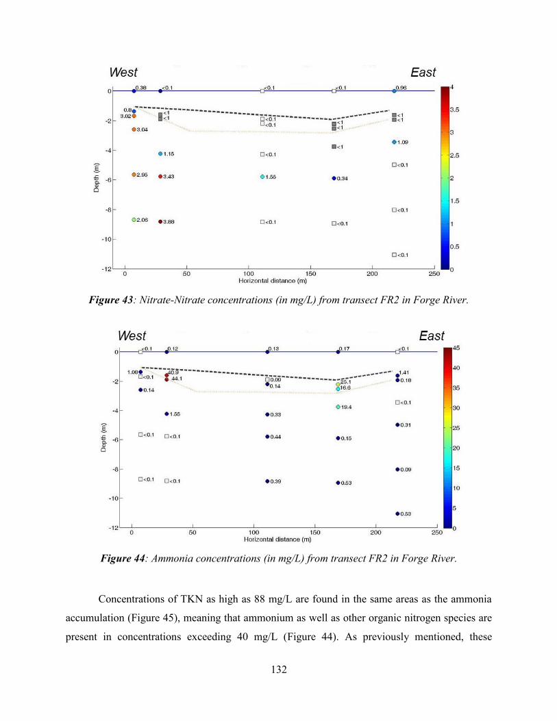
132

Figure 43: Nitrate-Nitrate concentrations (in mg/L) from transect FR2 in Forge River.

Figure 44: Ammonia concentrations (in mg/L) from transect FR2 in Forge River.

Concentrations of TKN as high as 88 mg/L are found in the same areas as the ammonia

accumulation (Figure 45), meaning that ammonium as well as other organic nitrogen species are

present in concentrations exceeding 40 mg/L (Figure 44). As previously mentioned, these

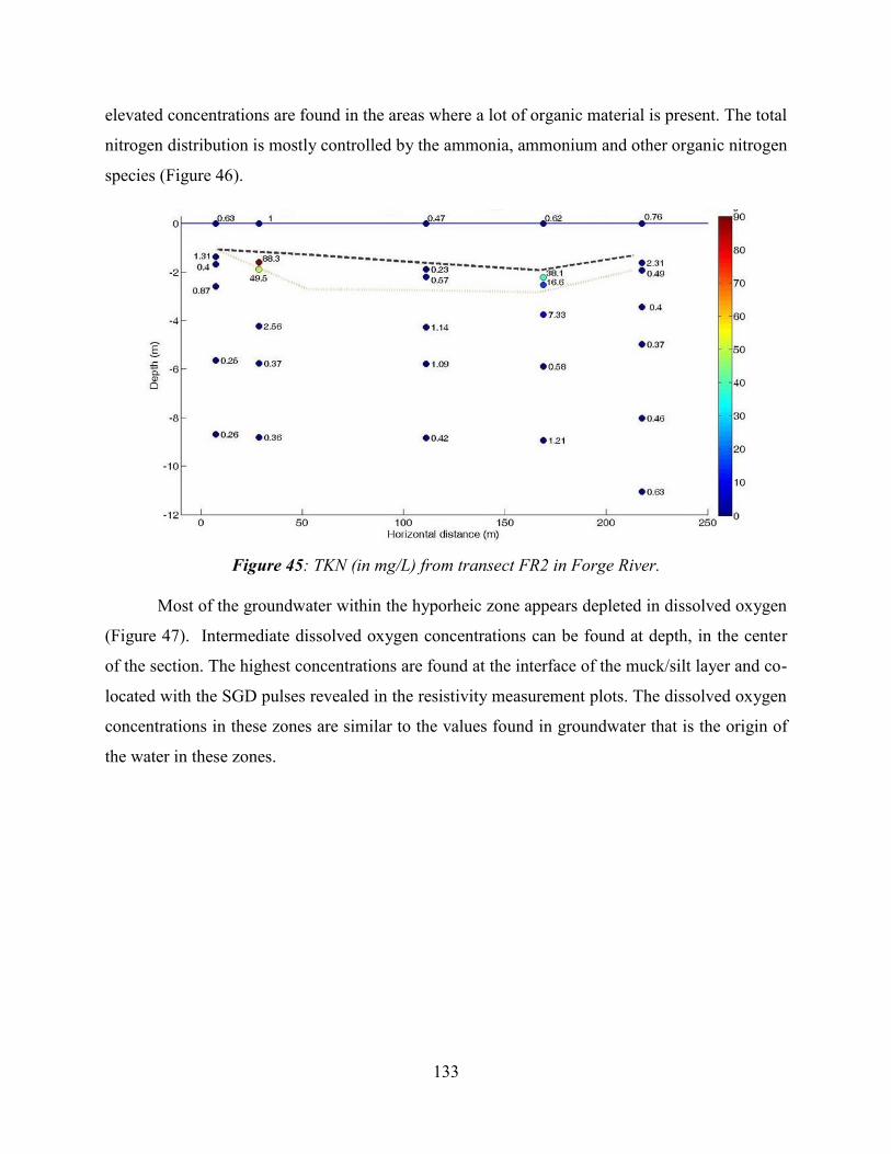
133

elevated concentrations are found in the areas where a lot of organic material is present. The total

nitrogen distribution is mostly controlled by the ammonia, ammonium and other organic nitrogen

species (Figure 46).

Figure 45: TKN (in mg/L) from transect FR2 in Forge River.

Most of the groundwater within the hyporheic zone appears depleted in dissolved oxygen

(Figure 47). Intermediate dissolved oxygen concentrations can be found at depth, in the center

of the section. The highest concentrations are found at the interface of the muck/silt layer and co-

located with the SGD pulses revealed in the resistivity measurement plots. The dissolved oxygen

concentrations in these zones are similar to the values found in groundwater that is the origin of

the water in these zones.

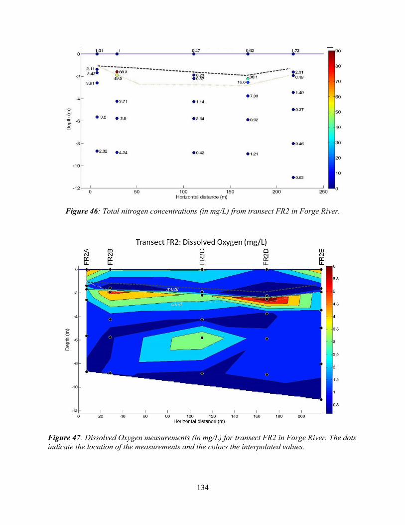
134

Figure 46: Total nitrogen concentrations (in mg/L) from transect FR2 in Forge River.

Figure 47: Dissolved Oxygen measurements (in mg/L) for transect FR2 in Forge River. The dots

indicate the location of the measurements and the colors the interpolated values.

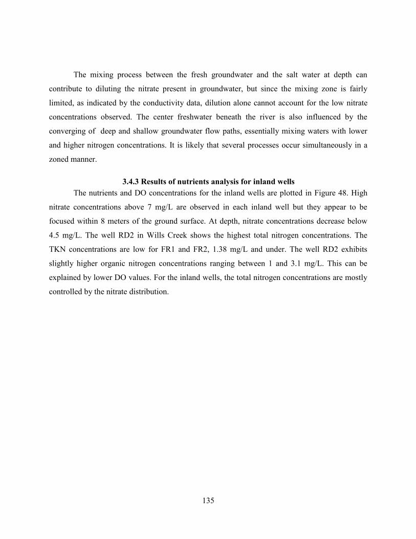
135

The mixing process between the fresh groundwater and the salt water at depth can

contribute to diluting the nitrate present in groundwater, but since the mixing zone is fairly

limited, as indicated by the conductivity data, dilution alone cannot account for the low nitrate

concentrations observed. The center freshwater beneath the river is also influenced by the

converging of deep and shallow groundwater flow paths, essentially mixing waters with lower

and higher nitrogen concentrations. It is likely that several processes occur simultaneously in a

zoned manner.

3.4.3 Results of nutrients analysis for inland wells

The nutrients and DO concentrations for the inland wells are plotted in Figure 48. High

nitrate concentrations above 7 mg/L are observed in each inland well but they appear to be

focused within 8 meters of the ground surface. At depth, nitrate concentrations decrease below

4.5 mg/L. The well RD2 in Wills Creek shows the highest total nitrogen concentrations. The

TKN concentrations are low for FR1 and FR2, 1.38 mg/L and under. The well RD2 exhibits

slightly higher organic nitrogen concentrations ranging between 1 and 3.1 mg/L. This can be

explained by lower DO values. For the inland wells, the total nitrogen concentrations are mostly

controlled by the nitrate distribution.

136

Figure 48: Nutrients analysis results for the inland wells RD2 in Wills Creek, and FR1 and FR2

at Forge River.

Note: Ammonia results are not shown as all samples were under the detection limit of 0.1 mg/L.

4. Conclusion

A significant portion of the freshwater flow of Forge River derives from groundwater,

which is transporting high concentrations of nutrients from the upland area to the river through

SGD. The complex nature of this discharge, its impact on the hyporheic zone and ultimately on

the surface waters are challenging to characterize. This study was able to define the most

predominant zones of SGD within the river as well as determine the distribution of different

nitrogen species and concentrations in these zones. Three distinct zones were identified and exist

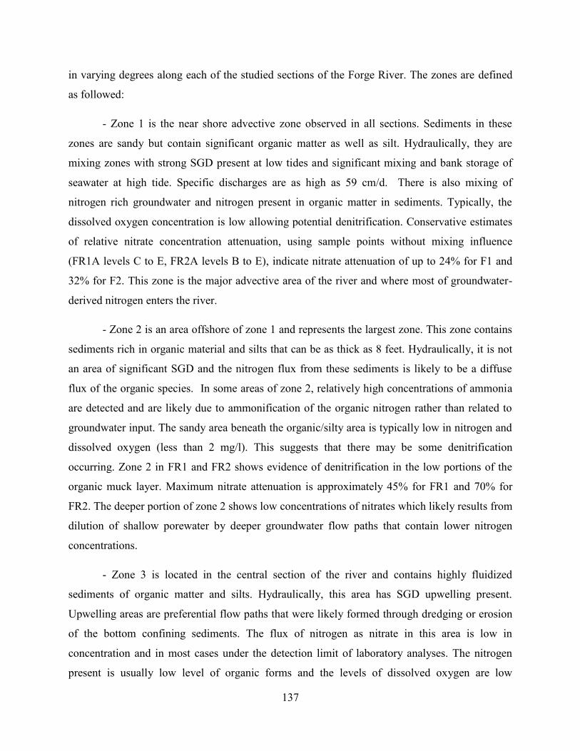
137

in varying degrees along each of the studied sections of the Forge River. The zones are defined

as followed:

- Zone 1 is the near shore advective zone observed in all sections. Sediments in these

zones are sandy but contain significant organic matter as well as silt. Hydraulically, they are

mixing zones with strong SGD present at low tides and significant mixing and bank storage of

seawater at high tide. Specific discharges are as high as 59 cm/d. There is also mixing of

nitrogen rich groundwater and nitrogen present in organic matter in sediments. Typically, the

dissolved oxygen concentration is low allowing potential denitrification. Conservative estimates

of relative nitrate concentration attenuation, using sample points without mixing influence

(FR1A levels C to E, FR2A levels B to E), indicate nitrate attenuation of up to 24% for F1 and

32% for F2. This zone is the major advective area of the river and where most of groundwater-

derived nitrogen enters the river.

- Zone 2 is an area offshore of zone 1 and represents the largest zone. This zone contains

sediments rich in organic material and silts that can be as thick as 8 feet. Hydraulically, it is not

an area of significant SGD and the nitrogen flux from these sediments is likely to be a diffuse

flux of the organic species. In some areas of zone 2, relatively high concentrations of ammonia

are detected and are likely due to ammonification of the organic nitrogen rather than related to

groundwater input. The sandy area beneath the organic/silty area is typically low in nitrogen and

dissolved oxygen (less than 2 mg/l). This suggests that there may be some denitrification

occurring. Zone 2 in FR1 and FR2 shows evidence of denitrification in the low portions of the

organic muck layer. Maximum nitrate attenuation is approximately 45% for FR1 and 70% for

FR2. The deeper portion of zone 2 shows low concentrations of nitrates which likely results from

dilution of shallow porewater by deeper groundwater flow paths that contain lower nitrogen

concentrations.

- Zone 3 is located in the central section of the river and contains highly fluidized

sediments of organic matter and silts. Hydraulically, this area has SGD upwelling present.

Upwelling areas are preferential flow paths that were likely formed through dredging or erosion

of the bottom confining sediments. The flux of nitrogen as nitrate in this area is low in

concentration and in most cases under the detection limit of laboratory analyses. The nitrogen

present is usually low level of organic forms and the levels of dissolved oxygen are low

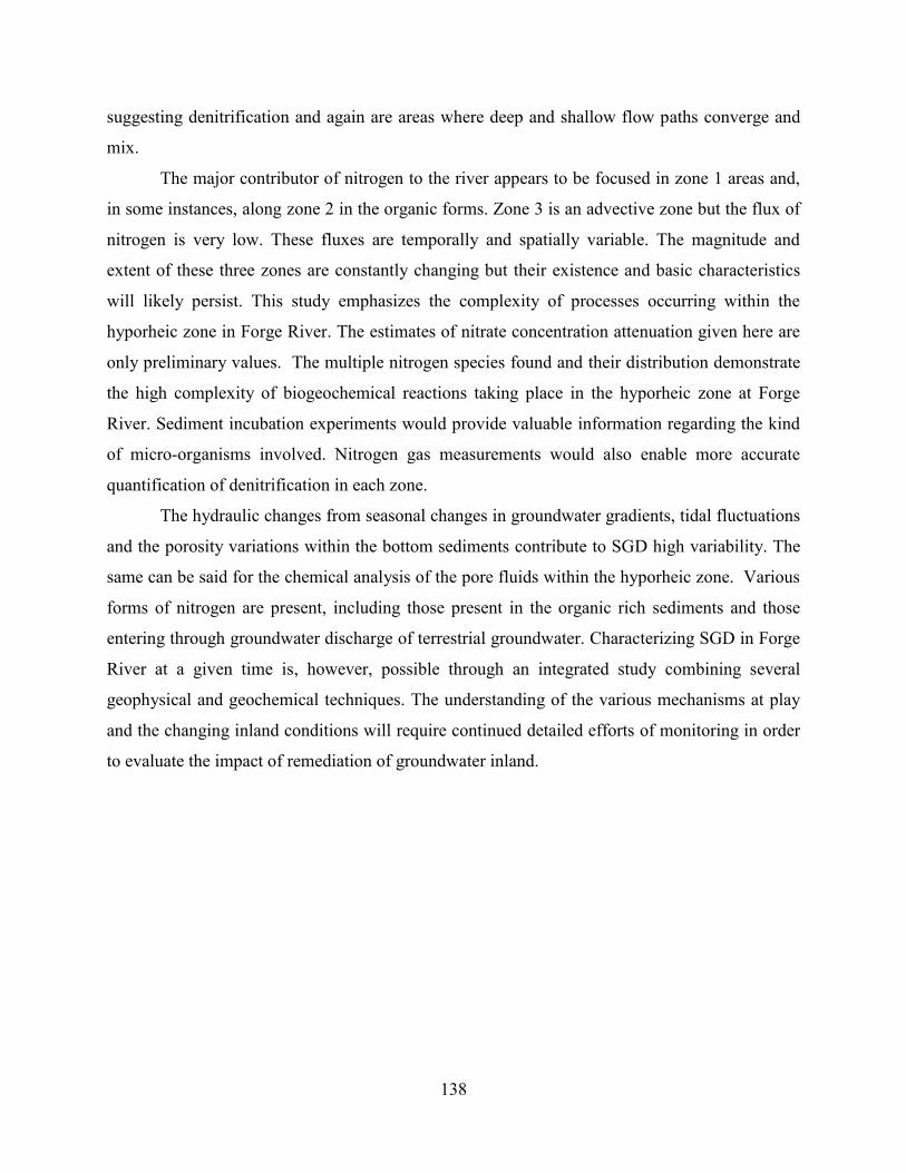
138

suggesting denitrification and again are areas where deep and shallow flow paths converge and

mix.

The major contributor of nitrogen to the river appears to be focused in zone 1 areas and,

in some instances, along zone 2 in the organic forms. Zone 3 is an advective zone but the flux of

nitrogen is very low. These fluxes are temporally and spatially variable. The magnitude and

extent of these three zones are constantly changing but their existence and basic characteristics

will likely persist. This study emphasizes the complexity of processes occurring within the

hyporheic zone in Forge River. The estimates of nitrate concentration attenuation given here are

only preliminary values. The multiple nitrogen species found and their distribution demonstrate

the high complexity of biogeochemical reactions taking place in the hyporheic zone at Forge

River. Sediment incubation experiments would provide valuable information regarding the kind

of micro-organisms involved. Nitrogen gas measurements would also enable more accurate

quantification of denitrification in each zone.

The hydraulic changes from seasonal changes in groundwater gradients, tidal fluctuations

and the porosity variations within the bottom sediments contribute to SGD high variability. The

same can be said for the chemical analysis of the pore fluids within the hyporheic zone. Various

forms of nitrogen are present, including those present in the organic rich sediments and those

entering through groundwater discharge of terrestrial groundwater. Characterizing SGD in Forge

River at a given time is, however, possible through an integrated study combining several

geophysical and geochemical techniques. The understanding of the various mechanisms at play

and the changing inland conditions will require continued detailed efforts of monitoring in order

to evaluate the impact of remediation of groundwater inland.

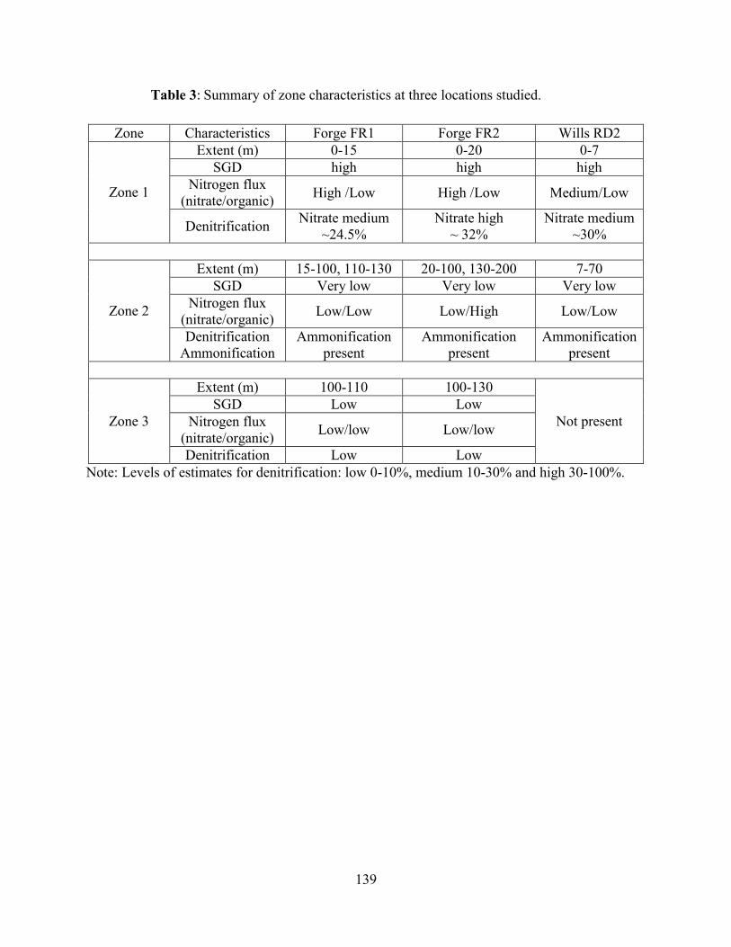
139

Table 3: Summary of zone characteristics at three locations studied.

Zone Characteristics Forge FR1 Forge FR2 Wills RD2

Zone 1

Extent (m) 0-15 0-20 0-7

SGD high high high

Nitrogen flux

(nitrate/organic) High /Low High /Low Medium/Low

Denitrification Nitrate medium

~24.5%

Nitrate high

~ 32%

Nitrate medium

~30%

Zone 2

Extent (m) 15-100, 110-130 20-100, 130-200 7-70

SGD Very low Very low Very low

Nitrogen flux

(nitrate/organic) Low/Low Low/High Low/Low

Denitrification

Ammonification

Ammonification

present

Ammonification

present

Ammonification

present

Zone 3

Extent (m) 100-110 100-130

Not present

SGD Low Low

Nitrogen flux

(nitrate/organic) Low/low Low/low

Denitrification Low Low

Note: Levels of estimates for denitrification: low 0-10%, medium 10-30% and high 30-100%.

140

References

Aller, R. C., C. J. Gobler, and B. J. Brownawell (2009), Data report on benthic flux studies

and the effect of organic matter remineralization in sediments on nitrogen and oxygen cycling in

the Forge River, New York: Task #1 and 2. Prepared for Suffolk County Department of Health

Services, Report, 62 pp.

Brownawell, B., D. Wang, J. Ruggieri, S. Sañudo-Wilhelmy, and R. L. Swanson (2009),

Sediment Quality Characterization for the Forge River, Long IslandRep., 21 pp, Prepared for the

Town of Brookhaven.

Burson, A. M., S. C. Talmage, and C. T. Gobler (2008), Linking the dynamics of nutrient

cycling and primary producers to hypoxia in Forge River, Mastic, NY, in SCERP Environmental

Symposium, edited, Stony Brook- Southampton, NY, USA.

Cameron Engineering and Associates (2012), Forge river management plan, LLP in

association with CH2MHill, prepared for the town of Brookhaven, Report.

Chadwick, D. B., J. Groves, C. Smith, and R. Paulsen (2003), Hardware description and

sampling protocols for the Trident Probe and UltraSeep systems: Technology to evaluate

contamination transfer between groundwater and surface water.Rep., United States Navy, SSC

San Diego.









Koike, I., and A. Hattori (1978), Denitrification and ammonia formation in anaerobic coastal

sediments, Applied and Environmental Microbiology, 35(2), 278-282.

Laroche, J., R. Nuzzi, R. Waters, K. Wyman, P. Falkowski, and D. Wallace (1997), Brown

Tide blooms in Long Island’s coastal waters linked to interannual variability in






141

Payne, W. (1973), Reduction of nitrogenous oxides by microorganisms, Bacteriological

Reviews, 37(4), 409.

Ryther, J. H. (1954), The ecology of phytoplankton blooms in Moriches Bay and Great

South Bay, Long Island, New York, The Biological Bulletin, 106(2), 198-209.

Wanlass, J. S. (2009), Development of an integrated geophysical and hydrological approach

to study submarine ground water discharge into Forge River, Stony Brook University, Stony

Brook.


Press Inc.

Zumft, W. G. (1997), Cell biology and molecular basis of denitrification, Microbiology and

Molecular Biology Reviews, 61(4), 533-616.

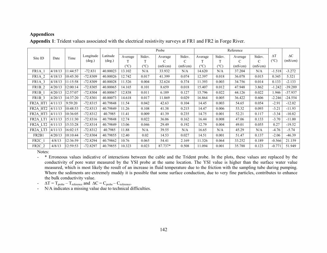
142

Appendices

Appendix 1: Trident values associated with the electrical resistivity surveys at FR1 and FR2 in Forge River.

Site ID Date Time Longitude

(deg.)

Latitude

(deg.)

Probe Reference

∆T

(°C)

∆C

(mS/cm) Average

T

(°C)

Stdev.

T

(°C)

Average

C

(mS/cm)

Stdev.

C

(mS/cm)

Average

T

(°C)

Stdev.

T

(°C)

Average

C

(mS/cm)

Stdev.

C

(mS/cm)

FR1A_1 4/18/13 11:44:57 -72.831 40.80023 13.102 N/A 33.932 N/A 14.620 N/A 37.204 N/A -1.518 -3.272

FR1A_2 4/18/13 10:45:30 -72.8309 40.80026 12.742 0.017 41.399 0.074 12.397 0.018 36.078 0.015 0.345 5.321

FR1A_3 4/18/13 11:15:58 -72.8309 40.80028 11.526 0.004 32.624 0.374 11.393 0.003 34.756 0.014 0.133 -2.133

FR1B_2 4/20/13 12:00:14 -72.8305 40.80065 14.165 0.101 8.659 0.018 15.407 0.012 47.948 3.862 -1.242 -39.289

FR1B_1 4/20/13 12:57:07 -72.8304 40.80067 12.838 0.011 6.189 0.127 15.796 0.022 44.126 0.022 1.946 -37.937

FR1B_3 4/20/13 14:37:20 -72.8301 40.80073 14.618 0.017 11.869 0.029 16.864 0.005 36.422 0.606 -2.246 -24.554

FR2A_HT1 4/11/13 9:59:20 -72.8315 40.79848 11.54 0.042 42.63 0.104 14.45 0.003 54.65 0.054 -2.91 -12.02

FR2A_HT2 4/11/13 10:48:53 -72.8313 40.79849 11.26 0.108 41.38 0.215 14.47 0.006 53.32 0.093 -3.21 -11.93

FR2A_HT3 4/11/13 10:36:05 -72.8312 40.7985 11.41 0.009 41.39 0.235 14.75 0.001 52.21 0.117 -3.34 -10.82

FR2A_LT1 4/11/13 15:11:30 -72.8316 40.79848 12.74 0.022 36.06 0.162 16.44 0.008 47.06 0.133 -3.70 -11.00

FR2A_LT2 4/11/13 15:33:28 -72.8314 40.79849 13.06 0.046 29.49 0.192 12.79 0.004 49.01 0.055 0.27 -19.52

FR2A_LT3 4/11/13 16:02:15 -72.8312 40.7985 11.88 N/A 39.55 N/A 16.65 N/A 45.29 N/A -4.76 -5.74

FR2B1 4/20/13 10:10:44 -72.8304 40.79855 12.40 0.02 14.53 0.027 14.51 0.001 51.47 0.137 -2.06 -46.39

FR2C_1 4/8/13 12:36:59 -72.8294 40.79862 10.76 0.065 54.41 2.169 11.326 0.064 33.252 0.189 -0.566 21.159

FR2C_2 4/8/13 12:59:53 -72.8297 40.79855 10.323 0.023 87.737* 0.508 11.094 0.001 35.788 0.123 -0.771 51.949

Notes:

- * Erroneous values indicative of interactions between the cable and the Trident probe. In the plots, these values are replaced by the

conductivity of pore water measured by the YSI probe at the same location. The YSI value is higher than the surface water value

measured, which is most likely the result of an increase in fluid temperature due to the friction with the sampling tube during pumping.

Where the sediments are extremely muddy it is possible that some surface conduction, due to very fine particles, contributes to enhance

the bulk conductivity value.

- ∆T = Tprobe – Treference and ∆C = Cprobe – Creference.

- N/A indicates a missing value due to technical difficulties.

143

Appendix 2: Trident results associated with the wells for transects FR1 and FR2, in Forge River.

Site

ID Date Time

Longitude

(deg.)

Latitude

(deg.)

Probe Reference

∆T

(°C)

∆C

(mS/cm)

Average

T

(°C)

Stdev

T

(°C)

Average

C

(mS/cm)

Stdev.

C

(mS/cm)

Average

T

(°C)

Stdev

T

(°C)

Average

C

(mS/cm)

Stdev.

C

(mS/cm)

FR1A 6/25/13 15:37:05 -72.8315 40.80065 18.851 0.001 6.655 0.03 28.491 0.022 27.444 0.617 -9.64 -20.789

FR1B 6/26/13 12:17:07 -72.8314 40.80075 19.436 0.020 7.927 0.033 27.653 0.026 38.249 0.593 -8.218 -30.322

FR1C 6/27/13 14:51:18 -72.8308 40.80093 12.812 0.002 4.804 0.006 17.165 0.002 2.43 0.002 -4.354 2.374

FR1D 7/9/13 11:23:18 -72.8304 40.80091 20.876 0.011 3.919 0.011 29.165 0.007 40.514 0.098 -8.289 -36.595

FR1E 7/9/13 13:10:49 -72.8302 40.8009 19.097 0.007 1.958 0.001 29.884 0.006 17.552 1.218 -10.79 -15.594

FR2A 6/20/13 9:48:14 -72.8316 40.79852 14.846 0.001 0.407 0.001 24.402 0.032 44.665 1.871 -9.556 -44.258

FR2B 6/19/13 11:19:30 -72.8311 40.79855 17.528 0.007 4.363 0.047 23.746 0.020 48.683 0.121 -6.218 -44.320

FR2C 6/24/13 14:54:30 -72.8306 40.79842 16.929 1.511 0.902 0.518 21.442 0.420 6.950 0.070 -4.513 -6.320

FR2D 6/21/13 11:08:27 -72.8298 40.79853 16.103 0.002 2.240 0.027 23.983 0.001 48.311 0.089 -7.880 -46.071

FR2E 6/20/13 12:17:04 -72.8292 40.79862 17.817 0.001 1.786 0.002 23.345 0.023 25.467 1.338 -5.527 -23.681

Notes:

- The name of a Trident station is built as follow: FR1/2 indicates the transect number, the letter A-E the associated well.

- C and T refer to conductivity and temperature, respectively.

- ∆T = Tprobe – Treference, and ∆C = Cprobe – Creference.

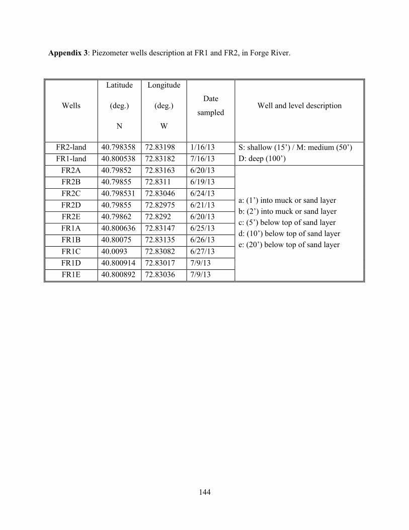
144

Appendix 3: Piezometer wells description at FR1 and FR2, in Forge River.

Wells

Latitude

(deg.)

N

Longitude

(deg.)

W

Date

sampled Well and level description

FR2-land 40.798358 72.83198 1/16/13 S: shallow (15’) / M: medium (50’)

D: deep (100’) FR1-land 40.800538 72.83182 7/16/13

FR2A 40.79852 72.83163 6/20/13

a: (1’) into muck or sand layer

b: (2’) into muck or sand layer

c: (5’) below top of sand layer

d: (10’) below top of sand layer

e: (20’) below top of sand layer

FR2B 40.79855 72.8311 6/19/13

FR2C 40.798531 72.83046 6/24/13

FR2D 40.79855 72.82975 6/21/13

FR2E 40.79862 72.8292 6/20/13

FR1A 40.800636 72.83147 6/25/13

FR1B 40.80075 72.83135 6/26/13

FR1C 40.0093 72.83082 6/27/13

FR1D 40.800914 72.83017 7/9/13

FR1E 40.800892 72.83036 7/9/13

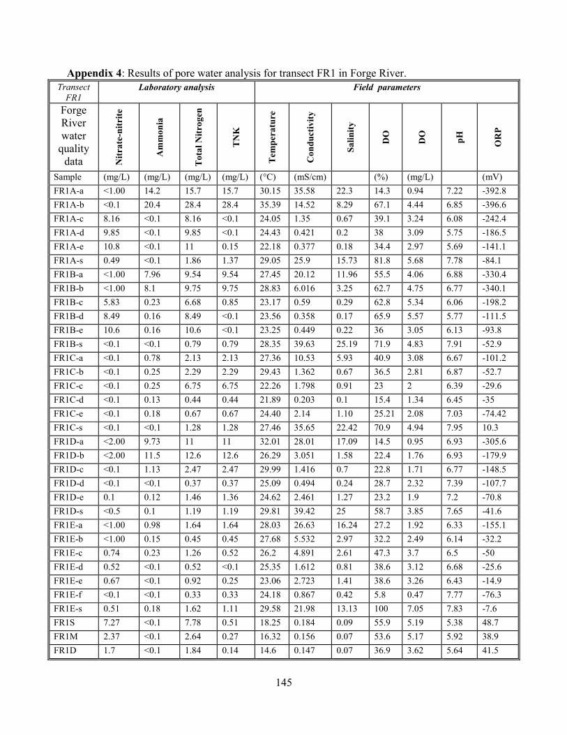
145

Appendix 4: Results of pore water analysis for transect FR1 in Forge River.

Transect

FR1 Laboratory analysis Field parameters

Forge

River

water

quality

data Nit

rate

-nit

rite

Am

mo

nia

To

tal

Nit

rog

en

TN

K

Tem

per

atu

re

Co

nd

uct

ivit

y

Sa

lin

ity

DO

DO

pH

OR

P

Sample (mg/L) (mg/L) (mg/L) (mg/L) (°C) (mS/cm) (%) (mg/L) (mV)

FR1A-a <1.00 14.2 15.7 15.7 30.15 35.58 22.3 14.3 0.94 7.22 -392.8

FR1A-b <0.1 20.4 28.4 28.4 35.39 14.52 8.29 67.1 4.44 6.85 -396.6

FR1A-c 8.16 <0.1 8.16 <0.1 24.05 1.35 0.67 39.1 3.24 6.08 -242.4

FR1A-d 9.85 <0.1 9.85 <0.1 24.43 0.421 0.2 38 3.09 5.75 -186.5

FR1A-e 10.8 <0.1 11 0.15 22.18 0.377 0.18 34.4 2.97 5.69 -141.1

FR1A-s 0.49 <0.1 1.86 1.37 29.05 25.9 15.73 81.8 5.68 7.78 -84.1

FR1B-a <1.00 7.96 9.54 9.54 27.45 20.12 11.96 55.5 4.06 6.88 -330.4

FR1B-b <1.00 8.1 9.75 9.75 28.83 6.016 3.25 62.7 4.75 6.77 -340.1

FR1B-c 5.83 0.23 6.68 0.85 23.17 0.59 0.29 62.8 5.34 6.06 -198.2

FR1B-d 8.49 0.16 8.49 <0.1 23.56 0.358 0.17 65.9 5.57 5.77 -111.5

FR1B-e 10.6 0.16 10.6 <0.1 23.25 0.449 0.22 36 3.05 6.13 -93.8

FR1B-s <0.1 <0.1 0.79 0.79 28.35 39.63 25.19 71.9 4.83 7.91 -52.9

FR1C-a <0.1 0.78 2.13 2.13 27.36 10.53 5.93 40.9 3.08 6.67 -101.2

FR1C-b <0.1 0.25 2.29 2.29 29.43 1.362 0.67 36.5 2.81 6.87 -52.7

FR1C-c <0.1 0.25 6.75 6.75 22.26 1.798 0.91 23 2 6.39 -29.6

FR1C-d <0.1 0.13 0.44 0.44 21.89 0.203 0.1 15.4 1.34 6.45 -35

FR1C-e <0.1 0.18 0.67 0.67 24.40 2.14 1.10 25.21 2.08 7.03 -74.42

FR1C-s <0.1 <0.1 1.28 1.28 27.46 35.65 22.42 70.9 4.94 7.95 10.3

FR1D-a <2.00 9.73 11 11 32.01 28.01 17.09 14.5 0.95 6.93 -305.6

FR1D-b <2.00 11.5 12.6 12.6 26.29 3.051 1.58 22.4 1.76 6.93 -179.9

FR1D-c <0.1 1.13 2.47 2.47 29.99 1.416 0.7 22.8 1.71 6.77 -148.5

FR1D-d <0.1 <0.1 0.37 0.37 25.09 0.494 0.24 28.7 2.32 7.39 -107.7

FR1D-e 0.1 0.12 1.46 1.36 24.62 2.461 1.27 23.2 1.9 7.2 -70.8

FR1D-s <0.5 0.1 1.19 1.19 29.81 39.42 25 58.7 3.85 7.65 -41.6

FR1E-a <1.00 0.98 1.64 1.64 28.03 26.63 16.24 27.2 1.92 6.33 -155.1

FR1E-b <1.00 0.15 0.45 0.45 27.68 5.532 2.97 32.2 2.49 6.14 -32.2

FR1E-c 0.74 0.23 1.26 0.52 26.2 4.891 2.61 47.3 3.7 6.5 -50

FR1E-d 0.52 <0.1 0.52 <0.1 25.35 1.612 0.81 38.6 3.12 6.68 -25.6

FR1E-e 0.67 <0.1 0.92 0.25 23.06 2.723 1.41 38.6 3.26 6.43 -14.9

FR1E-f <0.1 <0.1 0.33 0.33 24.18 0.867 0.42 5.8 0.47 7.77 -76.3

FR1E-s 0.51 0.18 1.62 1.11 29.58 21.98 13.13 100 7.05 7.83 -7.6

FR1S 7.27 <0.1 7.78 0.51 18.25 0.184 0.09 55.9 5.19 5.38 48.7

FR1M 2.37 <0.1 2.64 0.27 16.32 0.156 0.07 53.6 5.17 5.92 38.9

FR1D 1.7 <0.1 1.84 0.14 14.6 0.147 0.07 36.9 3.62 5.64 41.5

146

Appendix 5: Results of pore water analysis for transect FR2 in Forge River.

Transect

FR2 Laboratory analysis Field parameters

Forge

River

water

quality

data Nit

rate

-nit

rite

Am

mo

nia

To

tal

Nit

rog

en

TN

K

Tem

per

atu

re

Co

nd

uct

ivit

y

Sa

lin

ity

DO

DO

pH

OR

P

Sample (mg/L) (mg/L) (mg/L) (mg/L) (°C) (mS/cm) (%) (mg/L) (mV)

FR2A-a 0.8 1.08 2.11 1.31 24.75 20.72 12.39 26.2 2 5.94 8.4

FR2A-b 3.02 <0.1 3.42 0.4 23.73 1.989 1.01 34 2.85 5.9 49.1

FR2A-c 3.04 0.14 3.91 0.87 23.91 5.062 2.72 24.8 2.03 5.78 60.5

FR2A-d 2.95 <0.1 3.2 0.25 20.24 0.439 0.21 13.4 1.22 5.8 51.7

FR2A-e 2.06 <0.1 2.32 0.26 19.57 0.369 0.18 9.6 0.87 5.78 55.6

FR2A-s 0.38 <0.1 1.01 0.63 24.41 33.19 20.78 74.4 5.51 7.2 49.7

FR2B-a <1.00 40.9 88.3 88.3 26.42 35.9 22.61 4.1 0.3 7.02 -374

FR2B-b <1.00 44.1 49.5 49.5 27.93 8.045 4.44 66.9 5.36 7.12 -342.6

FR2B-c 1.15 1.55 3.71 2.56 21.76 7.16 3.93 13.9 1.11 6.13 -80

FR2B-d 3.43 <0.1 3.8 0.37 21.68 1.92 0.98 10 0.87 5.99 -30

FR2B-e 3.88 <0.1 4.24 0.36 20.24 0.431 0.21 11.4 1.09 6.12 -35

FR2B-s <0.1 0.12 1 1 24.61 43.86 28.29 45.5 3.21 7.35 -45.7

FR2C-a <0.1 <0.1 0.23 0.23 28.43 0.371 0.18 16.9 1.3 6.46 4.4

FR2C-b <0.1 0.14 0.57 0.57 27.21 2.624 1.34 51.4 3.68 7.64 3.1

FR2C-c <0.1 0.33 1.14 1.14 27.12 2.869 1.48 12 0.94 6.52 12.6

FR2C-d 1.55 0.44 2.64 1.09 25.31 27.77 17.06 54 4.03 6.89 -211.4

FR2C-e <0.1 0.39 0.42 0.42 26.58 41.78 26.75 11.3 0.79 7.14 -129.7

FR2C-s <0.1 0.13 0.47 0.47 32.18 44.66 28.37 60.1 3.14 7.69 -10.7

FR2D-a <1.00 25.1 38.1 38.1 28.79 22.68 13.61 2.1 0.14 7.43 -400.8

FR2D-b <1.00 16.6 16.6 16.6 27.1 7.369 4.51 88.8 6.85 7.76 -278.1

FR2D-c <1.00 19.4 7.33 7.33 24.5 5.899 3.2 10.9 0.86 6.95 -312.9

FR2D-d 0.34 0.15 0.92 0.58 21.43 9.855 5.56 13.4 1.1 6.66 -248.1

FR2D-e <0.1 0.53 1.21 1.21 23.44 30.9 19.21 18.8 1.4 6.89 -221.3

FR2D-s <0.1 0.17 0.62 0.62 24.63 11.04 28.42 25.3 1.79 7.15 -192.7

FR2E-a <1.00 1.41 2.31 2.31 24.19 38.03 24.15 11.6 0.84 7.01 -218.3

FR2E-b <1.00 0.18 0.49 0.49 23.18 5.847 3.17 27.1 2.26 6.81 -130.1

FR2E-c 1.09 <0.1 1.49 0.4 24.62 6.363 3.47 25.4 2.06 6.82 -14.1

FR2E-d <0.1 0.31 0.37 0.37 22.49 3.693 1.95 18.4 1.56 6.73 2.5

FR2E-e <0.1 <0.1 0.46 0.46 20.84 5.803 3.16 17 1.49 6.63 -5.4

FR2E-f <0.1 0.53 0.63 0.63 21.53 22.51 13.6 3 0.24 7.35 -141.5

FR2E-s 0.96 <0.1 1.72 0.76 24.37 20.57 12.29 62.5 4.87 7.07 16.1

FR2S 9.53 <0.1 9.85 0.32 17.73 0.268 0.13 35.9 3.35 4.6 77.7

FR2M 2.8 <0.1 3.17 0.37 15.72 0.172 0.08 60.3 5.74 5.95 41.9

FR2D 4.45 <0.1 5.83 1.38 16.12 0.723 0.35 55.2 5.32 5.97 40.1

147

Chapter 6: Conclusion and path forward

Conclusion

Spatio-temporal variations of submarine groundwater discharge (SGD) were investigated

using a suite of geophysical techniques. SGD distribution was characterized at the embayment

scale in Stony Brook Harbor, NY, a tidally-dominated low-energy environment with active mud

sedimentation. Numerical modelling simulations were utilized to verify the observed field

measurements in Stony Brook Harbor. Temporal variations of SGD in the intertidal zone were

investigated over a semi-diurnal tidal cycle in a partially confined sandy aquifer at West Neck

Bay, Shelter Island, NY. Finally, the relationship between nutrient fluxes and SGD were studied

at multiple locations along a contaminated tidal river, Forge River, NY.

To address the high spatial variability of SGD [Michael et al., 2005], we used an integrated

approach combining three or more hydrogeophysical methods [Burnett et al., 2006]. Electrical

resistivity (ER) surveys procured high spatial resolution 2D vertical cross-sections of

conductivity distribution, used as a proxy for salinity [Swarzenski et al., 2007; Swarzenski et al.,

2004]. Repeated over-time, ER surveys also delivered high temporal resolution images. A hand-

push conductivity and temperature (C/T) probe served to screen large areas by providing point

measurements used to identify zones of potentially fresh SGD, but also to obtain independent

measurements and verify the results of ER surveys [Chadwick et al., 2003]. Direct flow rate

measurements were collected using both ultrasonic [Paulsen et al., 2001] and manual [Lee,

1977] seepage meters, which allowed a high resolution investigation of tidally-driven SGD

variations. When possible, pore water samples were collected through piezometers to provide in

situ salinities and nutrients concentrations [Charette and Allen, 2006]. Finally, 2D density-

dependent steady-state numerical models of 2 contrasting sites in Stony Brook Harbor were

developed [Guo and Langevin, 2002; Zheng and Wang, 1999b].

Major conclusions of this thesis are summarized below:

1) My integrated approach using a direct-push probe ER surveys, C/T and seepage point

measurements, and porewater analyses was successful in identifying SGD spatio-

temporal variations at different scales and in various settings. Comparison between

148

methods revealed good agreement; in situ porewater conductivities confirmed the

reliability of ER surveys as a useful tool for studies in coastal environments.

2) Active deposition of low permeability mud sediments in low-energy coastal

environments has a significant impact on SGD distribution, as observed in Stony Brook

Harbor, NY. The mud layer acts as a cap: it restricts SGD at the shoreline, prevents

mixing with seawater and channels a significant volume of freshwater offshore. Areas

without mud show enhanced SGD and mixing with the overlying seawater. SGD volume

through the mud cap is estimated to reach approximately 30% of SGD discharged at the

shoreline. The numerical models developed for two contrasting sites were in agreement

with field observations made in Stony Brook Harbor. The models show that a 50 cm thick

mud layer with a hydraulic conductivity of 0.01 m/d can significantly alter the

groundwater flow pattern, mixing between ground and surface waters and salinity

distribution at depth. Investigating the presence and characteristics of such a layer prior to

SGD studies in similar environments is necessary before any attempt of SGD estimates at

a regional scale.

3) Time-lapse ER surveys revealed important horizontal and vertical variations in

groundwater conductivities, which suggest a dynamic salinity distribution in the intertidal

zone. This disagrees with standard published numerical models for unconfined isotropic

homogeneous aquifers and therefore illustrates the need for more specific numerical

models [Robinson et al., 2007b]. At Shelter Island, the ER cross-sections did not provide

evidence of the existence of a suggested confining unit [Stieglitz et al., 2007], yet high

SGD rates found in the intertidal zone are in favor of a partially confined aquifer. The

temporal variability of conductivity distribution at depth, however, disagrees with the

presence of a continuous low permeability unit at depth.

4) At Forge River, three zones were identified and characterized in terms of flow rate,

porewater conductivity and porewater nitrogen concentrations. The first zone, composed

of near shore sandy areas exhibited high SGD and important mixing with saline surface

water; this zone also constituted the major area of nitrate input to the river. The second

zone included areas covered by low permeability silty and organic-rich sediments which

had very low SGD rates and limited mixing. Slower seepage rates were associated with

higher denitrification and diffusive nitrogen fluxes. The last zone encompassed highly

149

fluidized silty and organic-rich sediments located in the center of the river where fresh

groundwater upwelling was observed. The low nitrogen concentrations measured in this

zone were the result of dilution and mixing with water of longer flow paths. The third

zone is the result of anthropogenic activity, primarily dredging, that disturbed the low-

permeability silt layer and modified SGD by creating preferential flow paths in the center

of the river.

Path forward

The findings described in this work raised questions about certain aspects of SGD that could

benefit from further investigation. Suggested directions about future research are presented

below.

1) Fine particle low-permeability sediments are common in low-energy environment

[Bratton et al., 2007]. Studies have emphasized the role of geologic heterogeneities

[Russoniello et al., 2013] and sediment compressibility [Gardner and Wilson, 2006] on

SGD; however, there is still a paucity of data regarding the influence of active

sedimentation on SGD. The development a set of comparative density-difference

transient models including tidal forcing would enable researchers to determine which

conditions, i.e. combination of thickness and hydraulic conductivity, would significantly

affect SGD distribution in such settings. These models, coupled with particle-tracking

algorithms, could also provide valuable information on flow paths and residence times

which impact chemical budgets [Kuan et al., 2012].

2) Embayments are common on the USA Atlantic coast and elsewhere in the world and

account for a significant portion of the coast. Curved shorelines have been shown to

focus hydraulic gradients and enhance groundwater flow in lake settings [Mc Bride and

Pfannkuch, 1975]. Development of 3D models that combine the effect of a concave

shoreline and density-driven phenomena would highlight the fundamental differences

between discharge processes and composition in coastal embayments compared to

straight ocean shorelines and would therefore contribute to improved chemical mass

balances at regional scale.

150

3) The highly variable and widely distributed occurrence of SGD has hindered accurate

large scale mass balances. An integrated approach that combines modeling, regional field

data, such as thermal infrared remote sensing techniques, and ground-truthing detailed

field measurements would provide an excellent framework to better locate and quantify

SGD on a regional scale [Johnson et al., 2008; Kelly et al., 2013].

151

References





IAHS Press.










437.



Geological Survey.
















152








543-550.




Technology, 41(20), 7022-7029.

Swarzenski, P. W., W. Burnett, C. Reich, H. Dulaiova, R. Peterson, and J. Meunier (2004),

Novel geophysical and geochemical techniques used to study submarine groundwater discharge

in Biscayne Bay, Florida.




153

List of References


Iversion Software, Austin, TexasRep.

Aller, R. C., C. J. Gobler, and B. J. Brownawell (2009), Data report on benthic flux studies

and the effect of organic matter remineralization in sediments on nitrogen and oxygen cycling in

the Forge River, New York: Task #1 and 2. Prepared for Suffolk County Department of Health

ServicesRep., 62 pp.

Anderson, M. P. (2005), Heat as a ground water tracer, Groundwater, 43(6), 951-968.

Anderson, W. P., and R. E. Emanuel (2010), Effect of interannual climate oscillations on

rates of submarine groundwater discharge, Water Resources Research, 46(5).


experiment, International Hydrological Program (IHP), Scientific Commitee on Oceanic

Research (SCOR), Land OCean Interactions in the Coastal Zone (LOICZ). Rep., 26 pp





Badon-Ghyben, W. (1888), Notes on the probable results of well drilling near Amsterdam,

Tijdschrift van het Koninklijk Inst. van Ing. Den Haag, 21.



Beck, A. J., J. P. Rapaglia, J. K. Cochran, and H. J. Bokuniewicz (2007a), Radium mass-

balance in Jamaica Bay, NY: Evidence for a substantial flux of submarine groundwater, Marine

Chemistry, 106(3), 419-441.




22(2), 477-490.





Bokuniewicz, H., M. Taniguchi, T. Ishitoibi, M. Charette, M. Allen, and E. A. Kontar (2008),

Direct measurements of submarine groundwater discharge (SGD) over a fractured rock aquifer in

Flamengo Bay Brazil, Estuarine Coastal and Shelf Science, 76(3), 466-472.

154



Bratton, J. F., S. M. Colman, E. R. Thieler, and R. R. Seal (2002), Birth of the modern

Chesapeake Bay estuary between 7.4 and 8.2 ka and implications for global sea-level rise, Geo-

Marine Letters, 22(4), 188-197.

Bratton, J. F., J. K. Böhlke, F. T. Manheim, and D. E. Krantz (2004), Ground Water Beneath

Coastal Bays of the Delmarva Peninsula: Ages and Nutrients, Ground Water, 42(7), 1021-1034.





IAHS Press.

Bugna, G. C., J. P. Chanton, J. E. Cable, W. C. Burnett, and P. H. Cable (1996), The

importance of groundwater discharge to the methane budgets of nearshore and continental shelf

waters of the northeastern Gulf of Mexico, Geochimica et Cosmochimica Acta, 60(23), 4735-

4746.





Burson, A. M., S. C. Talmage, and C. T. Gobler (2008), Linking the dynamics of nutrient

cycling and primary producers to hypoxia in Forge River, Mastic, NY, in SCERP Environmental

Symposium, edited, Stony Brook- Southampton, NY, USA.



Cable, J. E., J. B. Martin, and J. Jaeger (2006), Exonerating Bernoulli? On evaluating the

physical and biological processes affecting marine seepage meter measurements, Limnology and

Oceanography: Methods, 4, 172-183.

Cameron Engineering and Associates (2012), Forge river management plan, LLP in

association with CH2MHill, prepared for the town of Brookhaven, Report.

Chadwick, D. B., J. Groves, C. Smith, and R. Paulsen (2003), Hardware description and

sampling protocols for the Trident Probe and UltraSeep systems: Technology to evaluate

contamination transfer between groundwater and surface water.Rep., United States Navy, SSC

San Diego.



155

Charette, M., W. Moore, and W. Burnett (2008), Uranium-and thorium-series nuclides as

tracers of submarine groundwater discharge, U-Th series nuclides in aquatic systems. Elsevier,

155-191.











289-300.

Cooper Jr, H. H. (1959), A hypothesis concerning the dynamic balance of fresh water and

salt water in a coastal aquifer, Journal of Geophysical Research, 64(4), 461-467.

Coppens, A. B. (1981), Simple equations for the speed of sound in Neptunian waters, The

Journal of the Acoustical Society of America, 69(3), 862-863.

Corbett, D. R., and J. E. Cable (2003), Seepage meters and advective transport in coastal

environments: Comments on “Seepage meters and Bernoulli's revenge” by EA Shinn, CD Reich,

and TD Hickey. 2002. Estuaries 25: 126–132, Estuaries and Coasts, 26(5), 1383-1387.

Cross, V., D. S. Foster, and J. F. Bratton (2010), Continuous resistivity profiling and

seismic-reflection data collected in 2006 from the Potomac River estuary, Virginia and

MarylandRep.




Dimova, N. T., P. W. Swarzenski, H. Dulaiova, and C. R. Glenn (2012), Utilizing

multichannel electrical resistivity methods to examine the dynamics of the fresh water–seawater

interface in two Hawaiian groundwater systems, Journal of Geophysical Research, 117(C2),

C02012.




156

Durand, J. M., and R. Paulsen (2014), Flow Patterns and Nutrient Loading Associated With

Submarine Groundwater Discharge in Forge River and Wills CreekRep., Town of Brookhaven,

CDM Smith.








437.



884-894.

Gibbes, B., C. Robinson, L. Li, D. Lockington, and H. Li (2008a), Tidally driven pore water

exchange within offshore intertidal sandbanks: Part II numerical simulations, Estuarine, Coastal







Gobler, C. J., and S. A. Sañudo-Wilhelmy (2001), Temporal variability of groundwater

seepage and brown tide blooms in a Long Island embayment, Marine Ecology Progress Series,

217, 299-309.

Gonneea, M. E., A. E. Mulligan, and M. A. Charette (2013), Climate‐driven sea level

anomalies modulate coastal groundwater dynamics and discharge, Geophysical Research Letters,

40(11), 2701-2706.

Gross, M. G. (1972), Characteristics and environmental quality of six north shore bays:

Nassau and Suffolk Counties, Long Island, New YorkRep. 14, Stony Brook, New York: Marine

Science Research Center, State University of New York.



Geological Survey.

157

Harbaugh, A. W., E. R. Banta, M. C. Hill, and M. G. McDonald (2000), MODFLOW-2000,

the US Geological Survey modular ground-water model: User guide to modularization concepts

and the ground-water flow process, US Geological Survey Reston, VA, USA.

Heiss, J. W., W. J. Ullman, and H. A. Michael (2014), Swash zone moisture dynamics and

unsaturated infiltration in two sandy beach aquifers, Estuarine, Coastal and Shelf Science, 143,

20-31.




18(1), 173-185.

Herzberg, D. (1901), Die wasserversorgung einiger nordseebäder.

Hirsch, J., and A. Randazzo (2000), Hydraulic seepage within an astatic karst lake, North-

Central Florida'.



75-139.

Hwang, D.-W., G. Kim, Y.-W. Lee, and H.-S. Yang (2005), Estimating submarine inputs of

groundwater and nutrients to a coastal bay using radium isotopes, Marine Chemistry, 96(1), 61-

71.










Kohout, F. (1965), Section of geological sciences: a hypothesis concerning cyclic flow of

salt water related to geothermal heating in the floridan aquifer, Transactions of the New York

Academy of Sciences, 28(2 Series II), 249-271.

Koike, I., and A. Hattori (1978), Denitrification and ammonia formation in anaerobic coastal

sediments, Applied and Environmental Microbiology, 35(2), 278-282.

158






Kroeger, K., and M. Charette (2008), Nitrogen biogeochemistry of submarine groundwater

discharge, Limnology and Oceanography, 53(3), 1025-1039.

Krupa, S. L., T. V. Belanger, H. H. Heck, J. T. Brock, and B. J. Jones (1998), Krupaseep—

The next generation seepage meter, Journal of Coastal Research, 210-213.



Langevin, C. D., W. B. Shoemaker, and W. Guo (2003), MODFLOW-2000, the US

Geological Survey Modular Ground-Water Model--Documentation of the SEAWAT-2000

Version with the Variable-Density Flow Process (VDF) and the Integrated MT3DMS Transport

Process (IMT), US Department of the Interior, US Geological Survey.

Laroche, J., R. Nuzzi, R. Waters, K. Wyman, P. Falkowski, and D. Wallace (1997), Brown

Tide blooms in Long Island’s coastal waters linked to interannual variability in groundwater

flow, Global Change Biology, 3(5), 397-410.



Lewandowski, J., K. Meinikmann, T. Ruhtz, F. Pöschke, and G. Kirillin (2013), Localization

of lacustrine groundwater discharge (LGD) by airborne measurement of thermal infrared

radiation, Remote Sensing of Environment, 138, 119-125.

Lewis, E., and R. Perkin (1981), The practical salinity scale 1978: Conversion of existing

data, Deep Sea Research Part A. Oceanographic Research Papers, 28(4), 307-328.

Lewis, J. B. (1987), Measurements of groundwater seepage flux onto a coral reef: Spatial

and temporal variations, Limnology and Oceanography, 32(5), 1165-1169.



Libelo, E. L., and W. G. MacIntyre (1994), Effects of surface-water movement on seepage-

meter measurements of flow through the sediment-water interface, Applied Hydrogeology, 2(4),

49-54.

Lubke, E. R. (1964), Hydrogeology of the Huntington-Smithtown area, Suffolk County,

New York, U. S. Geological Survey Water-Supply Paper(1669-D), 68 p.

159



233-236.

Manheim, F. T., D. E. Krantz, and J. F. Bratton (2004), Studying ground water under

Delmarva coastal bays using electrical resistivity, Groundwater, 42(7), 1052-1068.



110-127.

Marshall, T. J., J. W. Holmes, and C. W. Rose (1996), Soil physics, Cambridge University

Press.

Martin, J. B., J. E. Cable, P. W. Swarzenski, and M. K. Lindenberg (2004), Enhanced

Submarine Ground Water Discharge from Mixing of Pore Water and Estuarine Water, Ground

Water, 42(7), 1000-1010.





Lett, 30(6), 1297.










21552.



Mulligan, A. E., and M. A. Charette (2006), Intercomparison of submarine groundwater

discharge estimates from a sandy unconfined aquifer, Journal of Hydrology, 327(3-4), 411-425.

Mulligan, A. E., R. L. Evans, and D. Lizarralde (2007), The role of paleochannels in

groundwater/seawater exchange, Journal of hydrology, 335(3), 313-329.

160

Mulligan, A. E., C. Langevin, and V. E. A. Post (2011), Tidal Boundary Conditions in

SEAWAT, Ground Water.

Murphy III, W., W. B. Ward, B. Boyd, G. Fleming, W. Murphy IV, R. Nolen-Hoeksema, M.

Art, and D. A. Rosales (2011), High-resolution shallow geophysics and geology in the Hudson-

Raritan Estuary Ecosystem Restoration, New Jersey, The Leading Edge, 30(2), 182-190.




Brook.

O'Rourke, D., P. R., and W. T-f. (1999), Measuring Submarine Groundwater Seepage Using

an Ultrasonic Flow meter and the "Drum Method"- A Comparative study, in Geology of Long

Island and Metropolitan New York, edited, Stony Brook, NY, USA.




2, 298-305.

Park, M. J. (1985), Prediction of tidal hydraulics and sediment transport patterns in Stony

Brook Harbor, State University of New York, Stony Brook.












Payne, W. (1973), Reduction of nitrogenous oxides by microorganisms, Bacteriological

Reviews, 37(4), 409.



Post, V. E. A. (2005), Fresh and saline groundwater interaction in coastal aquifers: Is our

technology ready for the problems ahead?, Hydrogeology Journal, 13(1), 120-123.

161



Revil, A. (1998), Nature of surface electrical conductivity in natural sands, sandstones, and

clays, Geophys Res Lett, 25(5), 691-694.

Robbins, S. K. (1977), Stony Brook Harbor: an interdisciplinary analysis., Special report

Rep. 9, SUNY Stony Brook, Marine Sciences Research Center.



Robinson, C., L. Li, and D. Barry (2007a), Effect of tidal forcing on a subterranean estuary,


Robinson, C., L. Li, and H. Prommer (2007b), Tide-induced recirculation across the aquifer-




C09007.

Robinson, C., P. Xin, L. Li, and D. A. Barry (2014), Groundwater flow and salt transport in

a subterranean estuary driven by intensified wave conditions, Water Resources Research, 50(1),

165-181.

Rosenberry, D. O. (2008), A seepage meter designed for use in flowing water, Journal of

Hydrology, 359(1), 118-130.

Rosenberry, D. O., and R. H. Morin (2004), Use of an electromagnetic seepage meter to

investigate temporal variability in lake seepage, Groundwater, 42(1), 68-77.

Rumer, R. R., and J. Shiau (1968), Salt water interface in a layered coastal aquifer, Water

Resources Research, 4(6), 1235-1247.




Ryther, J. H. (1954), The ecology of phytoplankton blooms in Moriches Bay and Great

South Bay, Long Island, New York, The Biological Bulletin, 106(2), 198-209.

Schubert, C. E. (1998), Areas contributing ground water to the Peconic estuary, and ground-

water budgets for the North and South forks and Shelter Island, Eastern Suffolk County, New

York.



162

Shinn, E. A., C. D. Reich, and T. D. Hickey (2002), Seepage meters and Bernoulli’s revenge,

Estuaries, 25(1), 126-132.






64-86.

Smith, A. J. (2004), Mixed convection and density‐dependent seawater circulation in coastal

aquifers, Water Resources Research, 40(8).

Soren, J. (1978), Hydrogeologic conditions in the town of Shelter Island, Suffolk County,

Long Island, New York., Water-Resources Investigation Report Rep. 77-77, U. S. Geological

Survey.

Stark, N., J. M. Durand, T.-f. Wong, J. Wanlass, and R. Paulsen (2012a), Submarine


Report for Site 2, Gardiners BayRep., Peconic Estuary Program of the Suffolk County

Department of Health Services.

Stark, N., J. M. Durand, T.-f. Wong, J. Wanlass, and R. Paulsen (2012b), Submarine


Report for Site 4, Bullhead BayRep., Peconic Estuary Program of the Suffolk County


Stark, N., J. M. Durand, T.-f. Wong, J. Wanlass, and R. Paulsen (2012c), Submarine


Report for Site 1, Three Mile HarborRep., Peconic Estuary Program of the Suffolk County


Stark, N., J. M. Durand, T.-f. Wong, J. Wanlass, and R. Paulsen (2012d), Submarine


Report for Site 3, Cedar PointRep., Peconic Estuary Program of the Suffolk County Department

of Health Services.

Stieglitz, T., M. Taniguchi, and S. Neylon (2008a), Spatial variability of submarine

groundwater discharge, Ubatuba, Brazil, Estuarine Coastal and Shelf Science, 76(3), 493-500.






543-550.

163




Technology, 41(20), 7022-7029.

Swarzenski, P. W., W. Burnett, C. Reich, H. Dulaiova, R. Peterson, and J. Meunier (2004),

Novel geophysical and geochemical techniques used to study submarine groundwater discharge

in Biscayne Bay, Florida.

Swarzenski, P. W., W. C. Burnett, W. J. Greenwood, B. Herut, R. Peterson, N. Dimova, Y.

Shalem, Y. Yechieli, and Y. Weinstein (2006), Combined time-series resistivity and geochemical

tracer techniques to examine submarine groundwater discharge at Dor Beach, Israel,




Taniguchi, M., and Y. Fukuo (1993), Continuous Measurements of Ground‐Water Seepage

Using an Automatic Seepage Meter, Groundwater, 31(4), 675-679.

Taniguchi, M., and H. Iwakawa (2001), Measurements of submarine groundwater discharge

rates by a continuous heat-type automated seepage meter in Osaka Bay, Japan, Journal of

Groundwater Hydrology, 43(4), 271-278.

Taniguchi, M., and H. Iwakawa (2004), Submarine groundwater discharge in Osaka Bay,

Japan, Limnology, 5(1), 25-32.



Taniguchi, M., T. Ishitobi, W. C. Burnett, and G. Wattayakorn (2007), Evaluating ground

water–sea water interactions via resistivity and seepage meters, Ground Water, 45(6), 729-735.




Tarantola, A. (2005), Inverse problem theory and methods for model parameter estimation,

siam.

Taylor, R. W., and D. S. Cherkauer (1984), The application of combined seismic and

electrical measurements to the determination of the hydraulic conductivity of a lake bed,

Groundwater Monitoring & Remediation, 4(4), 78-85.


Pr.

164

Top, Z., L. E. Brand, R. D. Corbett, W. Burnett, and J. Chanton (2001), Helium and radon as

tracers of groundwater input into Florida Bay, Journal of Coastal Research, 859-868.



Valiela, I., and C. Delia (1990), Special issue-groundwater inputs to coastal waters-

introduction, edited, Kluwer Academic Publ Spuiboulevard 50, Po Box 17, 3300 Aa Dordrecht,

Netherlands.






Coasts, 15(4), 443-457.

Wanlass, J. S. (2009), Development of an integrated geophysical and hydrological approach

to study submarine ground water discharge into Forge River, Stony Brook University, Stony

Brook.

Weinstein, Y., W. C. Burnett, P. W. Swarzenski, Y. Shalem, Y. Yechieli, and B. Herut

(2007), Role of aquifer heterogeneity in fresh groundwater discharge and seawater recycling: An

example from the Carmel coast, Israel, Journal of Geophysical Research-Oceans, 112(C12).



Winter, T., and H. Pfannkuch (1984), Effect of anisotropy and groundwater system

geometry on seepage through lakebeds: 2. Numerical simulation analysis, Journal of Hydrology,

75(1), 239-253.




Island North Shore Embayments, 165 pp, Stony Brook University.


Press Inc.

Zheng, C., and P. P. Wang (1999a), MT3DMS, A modular three-dimensional multi-species

transport model for simulation of advection, dispersion and chemical reactions of contaminants

in groundwater systems.

165




Zumft, W. G. (1997), Cell biology and molecular basis of denitrification, Microbiology and

Molecular Biology Reviews, 61(4), 533-616.

characterization of the spatial and temporal variations of ... · groundwater discharge using...

Documents