Characterization of shallow high-amplitude seismic anomalies in the HoopFault Complex, Barents Sea

Satinder Chopra1, Ritesh Kumar Sharma1, Graziella Kirtland Grech1, and Bent Erlend Kjølhamar2

Abstract

The shallow migrating hydrocarbon fluids in the western Barents Sea are usually found to be associated withhigh seismic amplitudes. We have attempted to characterize such shallow high-amplitude anomalies in the HoopFault Complex area of the western Barents Sea. The workflow is devised for discrimination of anomalies thatare associated with the presence of hydrocarbons from those that are not, and quantifying them further includesthe computation of a set of seismic attributes and their analyses. These attributes comprise coherence, spectraldecomposition, prestack simultaneous impedance inversion, and extended elastic impedance attributes, fol-lowed by their analysis in an appropriate crossplot space, as well as with the use of rock-physics templates.Finally, we briefly evaluate the futuristic efforts being devoted toward the integration of diverse data types suchas P-cable seismic as well as controlled-source electromagnetic data so as to come up with an integrated assess-ment for the prospects and to mitigate risk.

IntroductionMany areas of the western Barents Sea host shallow as

well as deep-seated hydrocarbon accumulations, where-from fluids are migrating to the seafloor (Bünz et al., 2012,2014; Bünz and Chand, 2013). Evidence of past episodesof gas migration can be seen in the form of pockmarks onthe seafloor as well as vertical pipes or chimneys on seis-mic sections (Plaza-Faverola et al., 2011). Natural gas hy-drates are also present in some areas (Chand et al., 2012),and free gas is present below the base of the hydrate sta-bility layer that is typically shallow. Such shallow migrat-ing hydrocarbon fluids as well as free gas below thehydrates represent potential hazards for drilling deeperwells and the construction of seabed installations. Thus,the detailed distribution of shallow migrating fluids or thepresence of gas in the shallow zones in the areas underinvestigation is required, for which data with high verticaland spatial resolution are required.

We begin by explaining succinctly the geologic settingof the western Barents Sea and in particular the HoopFault Complex (HFC) area we focus on. This is followedby our observations of high-amplitude anomalies on theshallow sections of the seismic data, whose characteriza-tion is our objective. With the water bottom starting atclose to 600 ms or so, the term “shallow” refers roughlyto the top one second of seismic data. Thereafter, we dis-cuss and present the results of a workflow that wasadopted for the discrimination of some of the high-ampli-

tude anomalies. This workflow entails the application ofcoherence, spectral decomposition, poststack impedanceinversion, going on to prestack simultaneous impedanceinversion and extended elastic impedance (EEI), fol-lowed by the analysis of the results in different crossplotspaces, using rock-physics templates (RPTs). The quan-titative interpretation workflow followed has helped ushigh-grade amplitude anomalies that are associated withhydrocarbons with a high level of confidence.

Finally, we briefly discuss the efforts being made inour industry for integration of seismic data with othertypes of data that are being acquired with state-of-the-art technology, all being aimed at mitigating explo-ration risk.

Geologic settingLocation

The Barents Sea forms part of the Arctic Ocean that isa continental shelf surrounded by islands, archipelagos,and peninsulas (Figure 1). It is bordered by the Svalbardand Franz Josef Land archipelagos to the north, the shelfedge toward the Norwegian-Greenland Sea, NovayaZemlya to the east, and the Norwegian Coast and KolaPeninsula to the south.

Basin evolutionThe western part of the Barents Sea (indicated with

the pink dashed square in Figure 1) can be divided into

1Arcis Seismic Solutions, Calgary, Canada and TGS, Asker, Norway. E-mail: Satinder.Chopra@tgs.com; Ritesh.Sharma@tgs.com; Graziella.KirtlandGrech@tgs.com.

2TGS, Asker, Norway. E-mail: benterlend.kjolhamar@tgs.com.Manuscript received by the Editor 13 March 2017; revised manuscript received 31 May 2017; published ahead of production 09 August 2017;

published online 05 October 2017. This paper appears in Interpretation, Vol. 5, No. 4 (November 2017); p. T607–T622, 26 FIGS.http://dx.doi.org/10.1190/INT-2017-0054.1. © 2017 Society of Exploration Geophysicists and American Association of Petroleum Geologists. All rights reserved.

t

Technical papers

Interpretation / November 2017 T607Interpretation / November 2017 T607

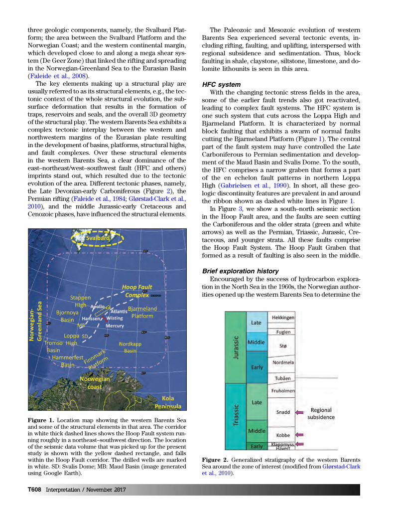
three geologic components, namely, the Svalbard Plat-form; the area between the Svalbard Platform and theNorwegian Coast; and the western continental margin,which developed close to and along a mega shear sys-tem (De Geer Zone) that linked the rifting and spreadingin the Norwegian-Greenland Sea to the Eurasian Basin(Faleide et al., 2008).

The key elements making up a structural play areusually referred to as its structural elements, e.g., the tec-tonic context of the whole structural evolution, the sub-surface deformation that results in the formation oftraps, reservoirs and seals, and the overall 3D geometryof the structural play. The western Barents Sea exhibits acomplex tectonic interplay between the western andnorthwestern margins of the Eurasian plate resultingin the development of basins, platforms, structural highs,and fault complexes. Over these structural elementsin the western Barents Sea, a clear dominance of theeast–northeast/west–southwest fault (HFC and others)imprints stand out, which resulted due to the tectonicevolution of the area. Different tectonic phases, namely,the Late Devonian-early Carboniferous (Figure 2), thePermian rifting (Faleide et al., 1984; Glørstad-Clark et al.,2010), and the middle Jurassic-early Cretaceous andCenozoic phases, have influenced the structural elements.

The Paleozoic and Mesozoic evolution of westernBarents Sea experienced several tectonic events, in-cluding rifting, faulting, and uplifting, interspersed withregional subsidence and sedimentation. Thus, blockfaulting in shale, claystone, siltstone, limestone, and do-lomite lithounits is seen in this area.

HFC systemWith the changing tectonic stress fields in the area,

some of the earlier fault trends also got reactivated,leading to complex fault systems. The HFC system isone such system that cuts across the Loppa High andBjarmeland Platform. It is characterized by normalblock faulting that exhibits a swarm of normal faultscutting the Bjarmeland Platform (Figure 1). The centralpart of the fault system may have controlled the LateCarboniferous to Permian sedimentation and develop-ment of the Maud Basin and Svalis Dome. To the south,the HFC comprises a narrow graben that forms a partof the en echelon fault patterns in northern LoppaHigh (Gabrielsen et al., 1990). In short, all these geo-logic discontinuity features are prevalent in and aroundthe ribbon shown as dashed white lines in Figure 1.

In Figure 3, we show a south–north seismic sectionin the Hoop Fault area, and the faults are seen cuttingthe Carboniferous and the older strata (green and whitearrows) as well as the Permian, Triassic, Jurassic, Cre-taceous, and younger strata. All these faults comprisethe Hoop Fault System. The Hoop Fault Graben thatformed as a result of faulting is also seen in the middle.

Brief exploration historyEncouraged by the success of hydrocarbon explora-

tion in the North Sea in the 1960s, the Norwegian author-ities opened up the western Barents Sea to determine the

Figure 1. Location map showing the western Barents Seaand some of the structural elements in that area. The corridorin white thick dashed lines shows the Hoop Fault system run-ning roughly in a northeast–southwest direction. The locationof the seismic data volume that was picked up for the presentstudy is shown with the yellow dashed rectangle, and fallswithin the Hoop Fault corridor. The drilled wells are markedin white. SD: Svalis Dome; MB: Maud Basin (image generatedusing Google Earth).

Figure 2. Generalized stratigraphy of the western BarentsSea around the zone of interest (modified from Glørstad-Clarket al., 2010).

T608 Interpretation / November 2017

hydrocarbon potential in the area. Beginning with somegas discoveries in 1980s, including the famous Snøhvitgas field in 1984 (being the first offshore developmentin the Barents Sea that came on-stream in 2007), andthe Goliat oil field discovered in 2000, and started pro-duction in March 2016.

The HFC is one of the core areas in the Norwegian23rd licensing round, and has been the focus area forseveral exploration companies since 2009.

The Wisting Central well 7324/8-1 drilled in 2013 andthe Hanssen well 7324/7-2 drilled in 2014 proved light oilin Jurassic fault blocks 500–800 m below the seabed.Although the Apollo well 7324/2-1 drilled (to a depthof 1050 m or so reaching just below the Stø Formation)in June 2014 came out dry, the Atlantis well 7325/1-1drilled (to a depth of 2800 m penetrated well belowthe Kobbe Formation) in July 2014, and the Mercurywell 7324/9-1 drilled in August 2015, re-sulted in small gas discoveries.

Prospective reservoir rocks in HFCAs mentioned above, post-Eocene ero-

sion removed much of Cretaceous andsome younger strata in the HFC area,making the older strata open for explora-tion. In some areas of the HFC, theCarboniferous and Permian units areshallow enough to be considered as ex-ploration targets. Carbonate rocks thatexperienced erosion and developed goodporosity are also possible targets.

The deltaic deposits of the Triassiccan be seen on the seismic data aslarge-scale northwest-prograding clino-form packages thinning in that direction.The sandstone channels in the Klapp-myss, Kobbe, and Snadd Formations(purple arrows in Figure 2) are prospec-tive in the HFC. Figure 4 shows a seg-ment of a seismic section CC′. Besidethe bright amplitude anomalies thatstand out on the section, the clinoformsignatures are also clearly seen.

The Atlantis well 7325/1-1 tested theTriassic section in a large closure adja-cent to the Hoop Graben. Although themain target was the Middle TriassicKobbe Formation, the well made a smalldiscovery in the Upper Triassic sands.Shallow stratigraphic boreholes drillednear the Svalis Dome have confirmedthe Middle Triassic Steinkobbe Memberof the Kobbe Formation as an excellentquality oil-prone marine source rock. Aswell, large deltaic channel systems ofthe Upper Triassic Snadd Formationcan be seen as bright amplitude anoma-lies on the seismic data.

Based on the exploration work carried out so far, theJurassic succession in the HFC area has been the mostsuccessful. The Upper Jurassic Hekkingen Formation(Figure 2) source rock is believed to be mature alongthe western and southern flanks of the basins adjacentto the HFC. The two recent wells, Wisting Central andHanssen proved oil in the Jurassic fault blocks between500 and 800 m below the seafloor. Both these discov-eries were supported by bright amplitude anomalieson the seismic.

Availability of seismic data and workflow adoptedA portion (500 km2) of the 3D seismic volume cover-

ing more than 22;000 km2 in and around the HFC waspicked up for carrying out a feasibility analysis aimed atcharacterizing the bright seismic amplitude anomalies,and also examining the fault and channel features in

Figure 4. Crossline CC′ passing through Atlantis well showing the clinoforms(blue arrows) and the bright amplitude anomalies (green arrows) clearly (datacourtesy of TGS, Asker, Norway).

Figure 3. A representative south–north seismic section in the Hoop Fault area.The area has a condensed geologic succession visible here from a Devonian orolder seismic basement to the Lower Cretaceous with a thin Quaternary cover.The main reservoir-prone units are Permian karstified carbonates, Mid-Triassicand Upper Triassic sandstones, Lower to Mid-Jurassic sandstones, and poten-tially Barremian sandstones. The main source rocks are of Mid-Triassic andUpper Jurassic age.

Interpretation / November 2017 T609

detail. A straightforward choice for accomplishing thiswas to put the data through poststack impedance inver-sion and generate one or more discontinuity attributessuch as coherence and curvature. Thus, the objectivesset for the exercise were (1) to use impedance inversionto follow potential reservoir leads within the Stø(Mid-Jurassic) and Kobbe (Mid-Triassic) Formations,(2) detect the potential prospects associated with directhydrocarbon indicators (DHIs), and (3) study the arealextent of the potential reservoirs present in the intervalof interest.

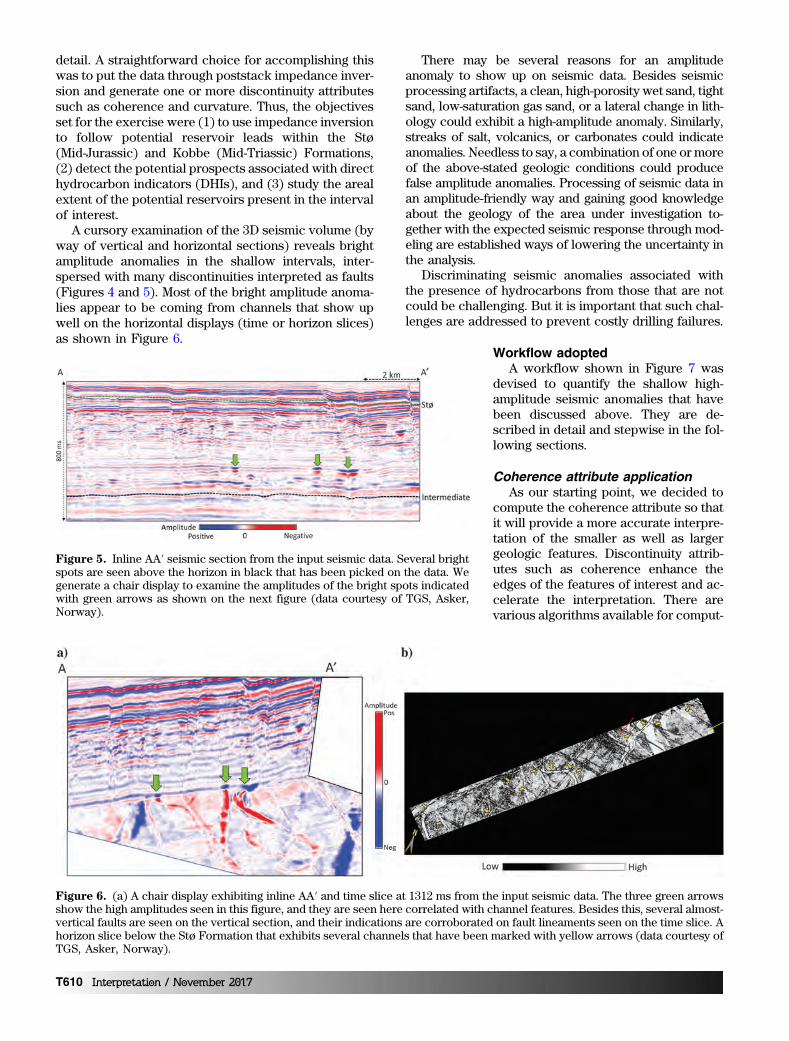
A cursory examination of the 3D seismic volume (byway of vertical and horizontal sections) reveals brightamplitude anomalies in the shallow intervals, inter-spersed with many discontinuities interpreted as faults(Figures 4 and 5). Most of the bright amplitude anoma-lies appear to be coming from channels that show upwell on the horizontal displays (time or horizon slices)as shown in Figure 6.

There may be several reasons for an amplitudeanomaly to show up on seismic data. Besides seismicprocessing artifacts, a clean, high-porosity wet sand, tightsand, low-saturation gas sand, or a lateral change in lith-ology could exhibit a high-amplitude anomaly. Similarly,streaks of salt, volcanics, or carbonates could indicateanomalies. Needless to say, a combination of one ormoreof the above-stated geologic conditions could producefalse amplitude anomalies. Processing of seismic data inan amplitude-friendly way and gaining good knowledgeabout the geology of the area under investigation to-gether with the expected seismic response through mod-eling are established ways of lowering the uncertainty inthe analysis.

Discriminating seismic anomalies associated withthe presence of hydrocarbons from those that are notcould be challenging. But it is important that such chal-lenges are addressed to prevent costly drilling failures.

Workflow adoptedA workflow shown in Figure 7 was

devised to quantify the shallow high-amplitude seismic anomalies that havebeen discussed above. They are de-scribed in detail and stepwise in the fol-lowing sections.

Coherence attribute applicationAs our starting point, we decided to

compute the coherence attribute so thatit will provide a more accurate interpre-tation of the smaller as well as largergeologic features. Discontinuity attrib-utes such as coherence enhance theedges of the features of interest and ac-celerate the interpretation. There arevarious algorithms available for comput-

Figure 5. Inline AA′ seismic section from the input seismic data. Several brightspots are seen above the horizon in black that has been picked on the data. Wegenerate a chair display to examine the amplitudes of the bright spots indicatedwith green arrows as shown on the next figure (data courtesy of TGS, Asker,Norway).

Figure 6. (a) A chair display exhibiting inline AA′ and time slice at 1312 ms from the input seismic data. The three green arrowsshow the high amplitudes seen in this figure, and they are seen here correlated with channel features. Besides this, several almost-vertical faults are seen on the vertical section, and their indications are corroborated on fault lineaments seen on the time slice. Ahorizon slice below the Stø Formation that exhibits several channels that have been marked with yellow arrows (data courtesy ofTGS, Asker, Norway).

T610 Interpretation / November 2017

ing coherence, including crosscorrelation, semblance,eigendecomposition of covariant matrices, and a moregeneral computation than the eigendecompositionapproach called the energy-ratio method (Chopra andMarfurt, 2008). The eigendecomposition method isbased on the eigenvectors and eigenvalues of the ofthe covariance matrix generated for the unit cube madeup of the input parameters for coherence computations,and it is given as the ratio of the principal eigenvalue tothe sum of all the eigenvalues or the trace of the matrix.In the energy ratio algorithm, first the energy of the co-herent component of the input traces is calculated, fol-lowed by the energy of the input traces, which is thetotal energy. The coherence coefficient is then com-puted as the ratio of the energy of the coherent compo-nent to the total energy. Energy ratiocoherence yields more crisp images ofthe discontinuity features of interest.

After preconditioning the inputstacked data volume using structure-ori-ented filtering, we generated a coherenceattribute volume using the energy-ratioalgorithm. The results are clearer andcrisper in comparison with the othermethods. In Figure 8, we show a set oftime slices at 1004, 1292, and 1332 ms.Each of these displays shows severalfaults with orientations in the north-west–southeast and northeast–southwestdirections. In addition to the faults, sev-eral well-defined channels are also seen.

Even though our main objective is the characterization ofshallow high-amplitude anomalies in the area, becausethe coherence attribute defines the faults and the edgesof the channels very well, we overlay this attribute on theinversion attribute displays later for more effective visu-alization.

Spectral decomposition application as DHIindicator

Next, we explore the application of spectral decom-position to the data at hand. The decomposition of theseismic signal band into constituent frequencies is re-ferred to as spectral decomposition. It is a useful toolthat has important applications including differentia-tion of lateral and vertical lithologic and/or pore-fluid

Figure 7. Workflow adopted for discrimination of seismic anomalies.

Figure 8. Time slices from the coherence volume at (a) 1004, (b) 1292, and (c) 1332 ms. Faults with northwest–southeast andnortheast–southwest orientations are seen clearly. Several paleochannels of different width are also seen at these levels. Thelocation of the two wells, Apollo and Atlantis, are marked in red. The lines in blue marked as AA′ and BB′ are the location ofthe seismic sections that are displayed in subsequent figures (data courtesy of TGS, Asker, Norway).

Interpretation / November 2017 T611

changes such as the DHI indicator and seismic geomor-phological applications aimed at delineating strati-graphic traps.

In the context of DHIs, the basic premise is thatreflections from fluid-saturated rocks are frequency de-pendent (Dutta and Ode, 1983; Denneman et al., 2002).Goloshubin et al. (2006) find that such reflection coef-ficient (water/gas) ratios are three times stronger at14 Hz than at 50 Hz, and they suggest that the observedreflection amplitudes be used for detecting liquid-satu-rated areas in thin porous layers. In the presence of hy-drocarbons, the encasing formations selectively reflectparticular frequencies and not others, leading to highamplitudes on seismic sections. This is because higherfrequencies suffer higher attenuation while traversinghydrocarbon reservoirs. In the event that the reservoirsare thin, the tuning of reflections also exacerbatesthe amplitude responses from reservoirs. Castagna et al.(2003) demonstrate that the instantaneous spectralanalysis of seismic data shows that low-frequencymodes of the seismic wavefield provide useful informa-tion for the study of fluid-saturated rocks.

We used the matching pursuit spectral decomposi-tion method as described by Liu and Marfurt (2007).It assumes that each band-limited seismic trace can berepresented as a linear combination of either Ricker orMorlet wavelets. A wavelet dictionary is precomputedand comprises the zero phase wavelets and 90° phasewavelets with different frequencies (sampled at 0.1 Hzincrements), in fact forming a complex wavelet diction-ary. Using complex trace attribute analysis, the centertime for each candidate wavelet is estimated by the

peaks of the amplitude in the instantaneous envelope,and its average frequency is estimated by the instanta-neous frequency at the envelope peak. A search is per-formed over the user-defined range of frequencies andtime samples about the precomputed peak frequencyand peak envelope to obtain the wavelet frequency-timepair that best correlates with the data. The difference be-tween the analytic seismic trace and the matched com-plex wavelets is iteratively minimized in a least-squaressense. Each wavelet is then decomposed into its spectralmagnitude and phase components. The process is re-peated until the residual falls below a threshold that isconsidered to be the noise level. This way, the input seis-mic data are decomposed into the desired frequencycomponents at a desired increment. To validate the de-composition, one can sum up the spectral components toreconstruct the original data. Alternatively, one can bal-ance the magnitude spectrum prior to reconstruction, re-sulting in a spectrally balanced seismic image.

On analyzing the spectral magnitude data, we noticedthat many of the high-amplitude anomalies are associatedwith higher spectral amplitudes. In Figure 9a, we show anarbitrary line passing through the Apollo and Atlantiswells, from the input seismic volume, and we notice somehigh-amplitude anomalies. The location of the line is in-dicated in yellow in Figure 8a. We generate the equiv-alent spectral magnitude displays at 20 and 60 Hz, andthey are shown in Figure 9b and 9c. Notice the high-spectral-magnitude values seen at 20 Hz, but not onthe 60 Hz display, even though the bandwidth of thedata extends to greater than 80 Hz. The Apollo wellbeing drilled to a shallow depth does not reach the

Kobbe top level, but there is a definiteanomaly at the intermediate level. Thus,spectral decomposition serves as apreliminary tool for location of the high-amplitude anomalies that could be hy-drocarbon bearing, and we now proceedfurther to seek their confirmation.

Impedance inversion applicationWell-log data are used to tie the main

time horizons to the seismic data and de-fine the impedance bounds for eachlayer. For well-log correlation, a waveletneeds to extracted from the seismicdata, which was done using a statisticalprocess. In Figure 10, we show thewell log-to-seismic correlation for theAtlantis well, with the extracted waveletshown on top. The modeled synthetictraces generated from the impedancelog are in blue and are shown correlatedwith the seismic traces at the location ofthe well in red. A reasonably good cor-relation is seen between the two. It isnot 100%, and thus it lends support toour choice of wavelet extraction usinga statistical process. As impedance in-

Figure 9. (a) Segment of an arbitrary line passing through the Apollo and At-lantis wells from (a) seismic data and showing high-amplitude anomalies. Thedisplay contrast has been reduced somewhat to depict these anomalies clearly.The location of the arbitrary line is indicated in yellow in Figure 8a. The equiv-alent segments of this arbitrary line extracted from 20 to 60 Hz volumes gener-ated using matching pursuit spectral decomposition, are shown in (b and c),respectively. Notice the anomalies indicated with yellow arrows exhibit highspectral magnitudes on the 20 Hz section and not on the 60 Hz section. TheApollo well being drilled to a shallow depth does not reach the Kobbe top level,but there is a definite anomaly at the intermediate level (data courtesy of TGS,Asker, Norway).

T612 Interpretation / November 2017

version is usually carried out in narrow time windows;the attenuation effects of the wavelet frequency arenegligible, but we do account for it in the next section.

We make use of a model-based poststack impedanceinversion to transform the seismic amplitude volumeinto an impedance volume. As the name implies, thestarting model is a low-frequency impedance model thatwas generated using the Atlantis wellthat extended through the formationsof interest. Horizons corresponding tothe Stø and Kobbe top formations wereused to constrain the low-frequencymodel with another pickable horizon inbetween, called the intermediate (shownin black in Figure 5). Because only onewell was used for constructing the low-frequency model, the impedance withineach layer may vary vertically, but it istaken as being constant laterally. In themodel-based inversion process, the start-ing model is compared with the inputseismic data, and the error betweenthem is iteratively minimized in a least-squares sense.

A segment of the inverted P-imped-ance section along line CC′ (the locationis displayed in Figure 8) is shown inFigure 11. Notice that the high seismicamplitudes marked in green are associ-ated with low impedance values. Weagain show the high-amplitude anoma-lies along line BB′ in Figure 12, whichalso exhibits a stratal grid that is usedfor displaying stratal slices. The term“stratal slice” may be clarified here. TheStø horizon was used to generate an-other phantom horizon approximately100 ms below it, and the interval dividedinto 10 proportional slices. The attributedisplayed along each such proportionalslice is referred to as a stratal slice. Thestratal slice at the location of the blue ar-row in Figure 12 is exhibited in Figure 13,which is a composite visual display ofimpedance and coherence attributes.Some of the channel features show lowimpedance values in dark blue and areindicated with light-blue arrows, andother channels show high impedance fillsas indicated with pale yellow arrows.Fault signatures are seen as black coher-ence lineaments.

The above workflow uses low imped-ance for screening out high seismicanomalies, and it may not be sufficientfor distinguishing bright amplitudeanomalies associated with hydrocarbonsfrom other geologic elements. For ana-lyzing these, we turned to the well-log

data for the Atlantis well in which dipole sonic and den-sity curves were available, and after computing differentattributes such as Lambda-rho and Mu-rho (Goodwayet al., 1997), we crossplotted them. On the Lambda-rhoversus Mu-rho crossplot (Figure 14), we noticed thatgas sand in the Snadd Formation exhibited low values ofLambda-rho and somewhat higher values of Mu-rho.

Figure 10. Well-to-seismic tie for Atlantis well. The wavelet extracted from theseismic data is shown above. The traces in blue are the modeled traces, and theseismic traces at the location of the well are in red.

Figure 11. Inverted P-impedance section with seismic overlay along crosslineCC′ passing through well Atlantis and displayed in Figure 8. The log curve over-laid in white is the computed P-impedance. The high seismic amplitudes markedin green are seen to be associated with lower impedance values (data courtesy ofTGS, Asker, Norway).

Figure 12. Inline BB′ with the overlay of the stratal slice grid. The stratal slicedisplayed in Figure 13 is indicated with blue arrows.

Interpretation / November 2017 T613

Besides, there was an overlap between the points repre-senting the gas sand and those coming from the Jurassic-Stø and Mid-Triassic Kobbe Formations. But by bringingdensity into our analysis, it was possible to discriminatebetween them. Thus, to extract Lambda-rho, Mu-rho, anddensity volumes from seismic data, we decided to runprestack simultaneous impedance inversion, in whichmultiple partial offset or angle substacks are invertedsimultaneously. For each angle stack, a unique waveletwas estimated from seismic data using a statistical

process. The extracted wavelets and their individual fre-quency spectra are shown in Figure 15. Prior to offset-to-angle domain conversion, the prestack seismic data inthe form of offset gathers were preconditioned by wayof background noise removal and trim static to enhancethe S/N. Subsurface low-frequency models for P-imped-ance, S-impedance, and density, constrained with theappropriate horizons in the broad zone of interest, areconstructed using the dipole sonic and density log dataavailable for the Atlantis well.

The simultaneous inversion processbegins with the low-frequency model,which is used to generate synthetictraces for the input partial angle stacks.Zoeppritz equations, or their approxima-tions, are used to estimate the band-limited elastic reflectivities. The angle-de-pendent wavelets are convolved with themodeled reflectivities for generating syn-thetic traces, which are then comparedwith corresponding real data traces. Themodel impedance values are iterativelytweaked in such a manner that the mis-match between the modeled angle gatherand the real angle gather is minimized ina least-squares sense. Because a differentwavelet is extracted for each partial an-gle stack and used in the inversion, theangle-dependent amplitude informationin the gather is used.

Once the background models, wave-lets, and partial stacks were obtained,inversion analysis was carried out atthe Apollo and Atlantis wells, which al-lows the optimization of the inversionparameters and validation. After per-forming it at well locations and obtainingsatisfactory results, prestack simultane-ous inversion was run for the full volumeto extract P-impedance, S-impedance,and density volumes. Even though it isan arduous task to extract density fromseismic data due to the unavailability ofnoise-free long-offset data, we could ex-tract it as the angle range for the availabledata extended to 47°–48°. Once we hadthe impedance volumes, Lambda-rho andMu-rho attributes were generated andthen we examined the anomalies in theLambda-rho-Mu-rho crossplot space.

The Lambda-rho and Mu-rho analysisis based on the assumption that Lamé’sfirst constant, Lambda (which is a proxyfor incompressibility) is sensitive topore fluid in the rock, and the other con-stant Mu (the modulus of rigidity) isonly influenced by the matrix material.Because gas is compressible, for a gassand, Lambda should be low, and Mu

Figure 13. Stratal slice as indicated in Figure 12 from the impedance volumewith the overlay of energy-ratio coherence. Notice the low impedance in blueseen in the channels indicated with cyan arrows and high impedance indicatedwith pale yellow arrows. Inline BB′ shown in the previous slide is also included inthe display (data courtesy of TGS, Asker, Norway).

Figure 14. Crossplot of Lambda-rho versus Mu-rho for the interval spanning theStø to Kobbe Formations. The cluster points are color coded with the fraction ofvolume clay. Cluster points enclosed in red (low Lambda-rho and high Mu-rho)and blue (low Lambda-rho and moderate Mu-rho) polygons are back-projectedand are seen to be coming from the Kobbe Formation and the Snadd Formation,with some overlap as well in between.

T614 Interpretation / November 2017

should be high (quartz is more rigid than shale). Thus,for a gas sand, we expect them to exhibit low values ofLambda-rho and high values of Mu-rho.

In Figure 16, we show segments of Lambda-rho andMu-rho sections passing through the Atlantis well, andwith the respective well-log curves overlaid. We noticetwo zones that stand out exhibiting low Lambda-rhoand highMu-rho, and they are highlighted in black. Theseindications are suggestive that they represent prospec-tive zones. We take this analysis forward through cross-plotting the two attributes (Lambda-rho and Mu-rho) andpicking up a cluster corresponding to low Lambda-rhoand high Mu-rho enclosed in Lamé red polygon andshown in Figure 17a. On back-projecting these enclosedpoints on the vertical (Figure 17b), we see the variationin the two zones that we have considered prospective.

A similar feasibility analysis was carried out for aninline passing through the Apollo well. Again, pickingup the high-amplitude anomalies on seismic, examiningthem in the Lambda-rho versus Mu-rho crossplot space,and back-projecting them on the vertical section, wesaw only the anomalies at the lower level as being pro-spective. We therefore concluded that all the high-am-plitude anomalies seen on the seismic data may not beassociated with hydrocarbons, and we need to examinethem with a different approach.

Because we were able to extract thedensity attribute also, in Figure 18 weshow the density section equivalent tothe Lambda-rho and Mu-rho sectionsshown in Figure 16. Notice that the low-density anomaly is indicated with theyellow arrow, but no density anomalyis seen at the lower level (the pink ar-row). Next, we crossplot density versusP-impedance as shown in Figure 19a forthe line passing through the Atlantiswell, and after enclosing the clusterpoints exhibiting low density and lowimpedance, and back-projecting, onlythe anomaly at the yellow arrow is seenhighlighted as shown in Figure 19b. Wetherefore conclude that we can trust thisanomaly as being associated with hydro-carbons.

Thus, by adopting a workflow thatentails the generation of P-impedance,S-impedance, and density attributes andexamining these attributes first in theLambda-rho versus Mu-rho crossplotspace, and then in the P-impedance ver-sus density crossplot space, it is possibleto identify the fluid-associated anomalies.

Impedance inversion after fre-quency balancing of seismic dataand analysis using RPTs

Aswe noticed in Figure 15, the spectrafor the wavelets extracted from the near-,

mid-, and far-angle stacks exhibit a lowering in frequencycontent as we go from the near- to far-angle stack, viathe mid-angle stack, as well as an overall roll off on

Figure 15. (a) Wavelets extracted the near-, mid-, and far-an-gle stacks; (b) frequency spectra for the wavelets extracted in(a). Notice the gradual reduction in the frequency content ingoing from the near- to the far-angle stack wavelets, as well asthe roll-offs on the higher frequency side.

Figure 16. Equivalent segments of sections passing through Atlantis well from(a) Lambda-rho and (b) Mu-rho attributes generated using prestack simultane-ous inversion. The individual curves overlaid are the Lambda-rho and Mu-rho logcurves on the respective sections. Notice the good correlation between the mea-sured and inverted attributes (data courtesy of TGS, Asker, Norway).

Interpretation / November 2017 T615

the higher frequency side. These effectsare a manifestation of the offset/angledependent attenuation as well as thechanges in the seismic wavelet withtime/depth. We decided to compensatefor this by balancing or flattening thespectra of the near-, mid-, and far-anglestack and bringing it to the same level.Our method of choice for this applicationwas the thin-bed reflectivity inversion,which has been described and illustratedelsewhere (Chopra et al., 2006; Puryearand Castagna, 2008). In this process, thetime-varying effect of the propagatingwavelet is removed from the seismic dataand the output of the spectral inversionprocess can be viewed as spectrallybroadened seismic data, retrieved in theform of broadband reflectivity that canbe filtered back to any desired band-width. This usually represents useful in-formation for interpretation purposes.Filtered thin-bed reflectivity, obtained byconvolving the reflectivity with a waveletof a known frequency band-pass, not onlyprovides an opportunity to study reflec-tion character associated with featuresof interest, but it also serves to confirmits close match with the original data.In Figure 20, we show the equivalentwavelets extracted from the same timewindow after frequency balancing. Pre-stack simultaneous impedance inversioncarried out with these wavelets and thebalanced near-, mid-, and far-angle stackyield higher resolution and thus leadto more accurate interpretation. In Fig-ure 21, we show the line CC′ from theP-impedance volumes before and afterthe balancing of the frequency spectrafor the wavelets extracted from thenear-, mid-, and far-angle stacks. Noticethe crisper look of the anomalies as wellas other events and their better standoutseen on the sections after frequencyspectra balancing.

Using RPTsØdegaard and Avseth (2004) intro-

duce the use of RPTs as an aid in inter-pretation of lithology and pore fluidinterpretation of well-log data and elas-tic inversion results. Since then, RPTshave become an effective tool for delin-eation of lithology and fluid content, avisual integration of well-log and seis-mic data and their calibration, leading toquantitative interpretation. Instead ofdefining arbitrary cut-off values for pro-

Figure 17. (a) Crossplot between Lambda-rho and Mu-rho attributes from theimpedance sections shown in Figure 16 passing through the Atlantis well.Although a high density of points form a cluster in the middle of the crossplot,there are some points that form a cluster deviating from it. These points re-present low values of Lambda-rho and high values of Mu-rho, which could beconsidered as representing prospective sandstones probably impregnated withgas. These points are enclosed in a red polygon as shown and back-projectedonto the vertical section as shown in (b). Notice the points are coming fromtwo different levels (red paintbrush patterns enclosed in dashed blue lines).

Figure 18. Equivalent segment of the profiles shown in Figure 16 passingthrough the Atlantis well, extracted from the density volume that is generatedusing prestack simultaneous inversion. The density log curve is overlaid on thesection. Notice the good correlation between the measured and inverted densityattribute (data courtesy of TGS, Asker, Norway).

T616 Interpretation / November 2017

spective intervals, RPTs help us definean accurate zone(s) for them.

These templates are first constructedor modeled from well-log data, usingtheoretical rock-physics principles forgeneration of trends for different lithol-ogies and fluids that may be expectedin the area. Once these are generated,they are used as an aid or guide for in-terpretation of elastic inversion-derivedattributes.

The well-log data measured in the At-lantis, well together with the petrophys-ical analysis carried out on it, furnishedthe data required for generation of theRPTs being used in this exercise.

The starting point for the generationof RPTs for the interval of interest is thepetrophysical analysis for calculation oflithologic and fluid composition, as wellas the porosity in the Atlantis well. Thenext step is the generation of porositytrends for the lithologies of interest, usu-ally based on the Hertz-Mindlin contacttheory (Mindlin, 1949) for pressuredependence of porosity (Ødegaard andAvseth, 2004). The porosity values rangefrom no porosity to the maximum poros-ity expected in the interval, of course us-ing the bulk and shear moduli of thesolid mineral comprising the dry rock.Between end values of porosity, themoduli for the dry rock are estimatedbased on the Hashin Shtrikman (HS)bounds (Hashin and Shtrikman, 1963)that allow the prediction of the effectiveelastic moduli of a mixture of grains andpores. The lower HS bound applies for unconsolidatedrocks, whereas cemented rocks are governed by theupper HS bound, both cases assuming isotropic andelastic rocks.

Finally, the dry rock parameters computed in theprevious two steps are input into Gassmann’s equationsto calculate saturated rock properties for brine and hy-drocarbons. In the present exercise, the reservoir fluidis water, gas, or their mixture. These computations al-low us to determine P-velocity, S-velocity, and density,and thus P-impedance and VP-VS ratio, which are thetypical output attributes from seismic elastic imped-ance inversion.

In Figure 22a, we show an RPTs overlaid on the cross-plot between the P-impedance and VP-VS ratio for theAtlantis well, for the interval between Stø and the HavertFormations. The cluster points are color coded withporosity values ranging from 5% to 25%. The clusters ofpoints with low impedance and low VP-VS ratio exhibithigh porosity and high gas saturation and are enclosed inred and purple polygons. When back-projected on to the

Figure 19. (a) Crossplot between the inverted density and P-impedance attrib-utes derived from the prestack simultaneous impedance inversion. The cluster ofpoints enclosed in the red polygon exhibit low density and low impedance and socould represent hydrocarbon fluids. On back-projecting these points on the ver-tical section as shown in (b), they highlight only the anomaly at the upper level,and not the lower one.

Figure 20. (a) Wavelets extracted the near-, mid-, and far-an-gle stacks and (b) frequency spectra for the wavelets extractedin (a). Notice the balancing of the frequency content for thenear-, mid-, and far-angle stack wavelets.

Interpretation / November 2017 T617

well-log curves as shown in Figure 22b, they highlight theintervals between the Stø and Kobbe markers.

In Figure 22c, we show a similar crossplot for the P-impedance and VP-VS ratio derived from prestack simul-taneous impedance inversion without frequency balanc-ing, with overlaid RPTs. Notice that the cluster of pointshas an overall shape that is similar to the one seen in thecrossplot shown in Figure 22a from the Atlantis well. Thedrawback we see is that the cluster points within the redand purple polygons are not spread out. In Figure 22d, weshow an equivalent crossplot from the two attributes de-rived from prestack simultaneous impedance inversionwith frequency balancing. Now we see a good spread ofcluster points within the red and purple polygons. Onbacktracking the cluster polygons within the differentpolygons on vertical seismic (Figure 23), we note thatthey highlight the high-amplitude anomalies at the Stø,Snadd, and Kobbe levels, which we have seen before.

EEI applicationAfter application of spectral decomposition as DHI

and prestack simultaneous impedance inversion, we de-cided to further quantify the hydrocarbon bearing zonesin our broad zone of interest. We pursue this exercisewith the application of the EEI approach.

Elastic impedance inversion is a generalization ofacoustic impedance for a variable angle of incidence,and it provides a consistent and absolute framework tocalibrate and invert non-zero-offset seismic data (Con-

nolly, 1999) for fluid discrimination and lithology predic-tion for reservoirs. However, the elastic impedancevalues decrease with the increasing angle of incidenceand require a scale factor varying angles if they wereto be compared with acoustic impedance values. Whit-combe (2002) not only introduces normalizing constantsto remove the variable dimensionality and overcame thisproblem, but also introduces EEI (Whitcombe et al.,2002), which broadens the definition of elastic imped-ance. According to this formulation, some of the rockproperties cannot be predicted by the elastic impedanceapproach that usually considers the angle of incidencerange as 0°–30°, which are the values taken by sin2 θ.Consequently, by bringing about a change of variable,i.e., sin2 θ replacedwith tanχ, the angle range is extendedfrom −90° to þ90°, and this allows calculation of animpedance value beyond physically observable range ofangle θ. The χ angle can be selected to optimize the cor-relation of the EEI curves with petrophysical reservoirparameters, such as Vclay, water saturation, and porosityor with elastic parameters such as bulk modulus, shearmodulus, Lamé constants, and so on. It may be noted thatχ is not the actual reflection angle, but it is an indepen-dent input variable that is required for computing EEI.

We illustrate the different steps followed in the EEIapproach in Figure 24a. Because EEI reflectivities arecrosscorrelatedwith desirable V clay and effective porositylog curves for different values of the angles, the correla-tion coefficients are plotted in Figure 24b. The maximum

positive correlation coefficient of 0.85 forVclay (green curve) is seen at an angle of28°, and a negative correlation coefficientof 0.9 at an angle of 22° (blue curve). Thevalues of angles allow the determinationof these properties (effective porosity andVclay) from seismic data through the ap-plication of Zoeppritz equations on seis-mic angle gathers.

In Figure 25a and 25b, we exhibitequivalent crossline sections from the ef-fective porosity and V clay volumes withthe respective petrophysical log curvesoverlaid on them. A reasonably goodmatch between them is seen in bothcases, which enhances our confidence inthe application of the followed approachfor the data at hand.

Next, we crossplotted the effectiveporosity and V clay derived attributes asshown in Figure 26a. On enclosing thecluster of points that exhibit high poros-ity and low values or not-so-low values ofVclay with red, green, and blue polygons,and back projecting on the vertical seis-mic, we are able to highlight these pointscoming from different zones. In Fig-ure 26b, we see the differentiation ofthe potential reservoirs within the three

Figure 21. Inline CC′ from the P-impedance volumes: (a) before and (b) afterfrequency balancing of the near-, mid-, and far-angle stacks. Notice the crisperlook of the anomalies as well as other events and their better stand-out seen onthe sections after frequency balancing.

T618 Interpretation / November 2017

formations of interest, namely, the Stø,Snadd, and Kobbe Formations.

All these attribute volumes generatedearlier, together with porosity and Vclaydata volumes helped us generate displaysat the levels of interest. This was a signifi-cant aid in studying the areal extent ofthe potential reservoirs present in the in-tervals of interest, which was the thirdobjective for our exercise.

Future directionsBesides improving the quality of the

existing seismic data through reprocess-ing (with the latest algorithms) and theirintegration with borehole data, the state-of-the-art acquisition of fresh data with

Figure 22. (a) Crossplot between the P-impedance and VP-VS ratio for data from Atlantis well, and for the interval between theStø and Kobbe markers, with an RPTs overlaid on it. The cluster of points with low impedance and low VP-VS ratio exhibit highporosity and high gas saturation and are enclosed in red and purple polygons. When back-projected onto the well-log curves asshown in (b), the highlight the intervals between Stø and Kobbe markers, (c) Crossplot between the P-impedance and VP-VS ratioderived from seismic prestack simultaneous impedance inversion before frequency enhancement, and for the interval between theStø and Kobbe markers. The same RPTs shown in (a) is overlaid on it. The cluster of points exhibit an overall shape similar tothe cluster we see for well data, but they do not seem scattered enough within the red and purple polygons, (d) Crossplot betweenthe P-impedance and VP-VS ratio derived from seismic prestack simultaneous impedance inversion after frequency enhancement,and for the interval between the Stø and Kobbe markers. The same RPTs shown in (a) is overlaid on it. The cluster of points exhibitan overall shape similar to the cluster we see for well data, but they are nowwell-scattered within the red and purple polygons, andthus they offer a more accurate interpretation.

Figure 23. The cluster of points enclosed in four different polygons seen in Fig-ure 22 back-projected on the vertical seismic section. Notice the anomalies seenat the Kobbe, Snadd, and Stø levels highlighted with purple and yellow.

Interpretation / November 2017 T619

more powerful acquisition technology are being carriedout in the Barents Sea.

Among the more powerful 3D marine seismic dataacquisition technologies available in the industry today,the patented P-cable multistreamer seismic system holdspromise in terms of resolution on the processed datathat is much greater than conventional 3D seismic data.The P-cable seismic data acquisition technology is aseismic method that uses the sensitivity of the seismicwave velocity and density of the medium for generatingthe data. The controlled-source electromagnetic methodmeasures the electrical conductivity of the medium andserves as an independent source of information generat-ing a volume of subsurface resistivity that can help locatepockets of hydrocarbon fluids. In that sense the two aredisparate exploration techniques, in which the processeddata are interpreted separately and the results integrated.

Natural hydrocarbon seepage on the seafloor couldbe due to vertical leakage of light oil or gas fromcharged reservoirs in the subsurface or a result ofhydrocarbons that have traveled long lateral distancesthrough vents or via porous zones or faults andreached the seafloor. Such seepage out of the seafloorcan alter the physical and biological characteristicsof the water-bottom sediments. Sometimes the seep-age of light hydrocarbons may not be physically de-tected, but as they diagenetically alter the rocks orshallow sediments through which they pass, theycan be detected chemically. If such seepage is physi-cally detected on the seafloor, it could serve as a DHI.Therefore, multibeam seafloor mapping and samplingis being done by some of the operators in that area.Plans are also underway for integrating all this datafor mitigating exploration risk.

Figure 24. (a) Workflow for the EEI approachfor predicting the volume of petrophysicalproperties from seismic data, (b) crosscorrela-tion analysis for effective porosity (blue curve)and Vclay (green curve) with EEI curves. Amaximum negative correlation is seen for effec-tive porosity at 22°, and a maximum positivecorrelation is seen for Vclay at 28°.

Figure 25. (a) A crossline section from in-verted effective porosity volume passingthrough a well. The overlaid effective porositycurve shows a strong correlation with invertedresults. (b) Equivalent crossline section frominverted Vclay volume passing through a well.The overlaid Vclay curve shows a strong corre-lation with inverted results (data courtesy ofTGS, Asker, Norway).

T620 Interpretation / November 2017

ConclusionWe have tried to characterize shallow bright ampli-

tude anomalies with the application of an extensiveworkflow that includes attribute applications such as co-herence, spectral decomposition, prestack simultaneousimpedance inversion, and EEI. This has allowed us to dis-criminate between the bright amplitude anomalies thatmay be prospective from others that could be exhibitinghigh amplitudes due to geologic conditions. Althoughmatching pursuit spectral decomposition helped us de-tect the signature of hydrocarbon-bearing anomaliesat low frequencies, the P-impedance, S-impedance, anddensity attributes derived from simultaneous impedanceinversion on analysis in crossplot space helped us highgrade the anomalies pertaining to hydrocarbon presence.

We quantified our anomaly analysis in P-impedanceversus VP-VS ratio crossplot space with overlaid RPTsas well as generation of petrophysical properties suchas porosity and Vclay volumes through application ofEEI. Those high-amplitude seismic anomalies exhibitinglow-frequency signatures, low Lambda-rho and high Mu-rho, low-density and low P-impedance, high porosity,low V clay fraction were considered prospective. Thoseanomalies that have been consistently highlighted withthe different techniques used elevate the level of our con-fidence in their interpretation.

The overall success of such a workflow would de-pend on the quality of the well and seismic data used.Besides, the availability of shear log data is desirablefor getting good results from simultaneous inversion,which even these days are not available.

AcknowledgmentsThe authors wish to thank B. Zhang and two anony-

mous reviewers for making suggestions that improved

the quality of this paper. The authorsalso wish to thank TGS for permissionto present this work.

ReferencesBünz, S., and S. Chand, 2013, Arctic gas-

hydrates on the Svalbard margin andin the Barents Sea: 73rd Annual Interna-tional Conference and Exhibition,EAGE, Extended Abstracts, doi: 10.3997/2214-4609.20131161.

Bünz, S., A. Plaza-Faverola, S. Hurter, andJ. Mienert, 2014, 4D seismic study ofactive gas seepage systems on theVestnesa Ridge, offshore W-Svalbard:EGU General Assembly ConferenceAbstracts, 16026.

Bünz, S., S. Polyanov, S. Vadakkepuliyam-batta, C. Consolaro, and J. Mienert, 2012,Active gas venting through hydrate-bear-ing sediments on the Vestnesa Ridge, off-shore W-Svalbard: Marine Geology, 332,189–197.

Castagna, J. P., S. Sun, and R. W. Siegfried, 2003, Instanta-neous spectral analysis: Detection of low-frequency shad-ows associated with hydrocarbons: The Leading Edge,22, 120–127, doi: 10.1190/1.1559038.

Chand, S., T. Thorsnes, L. Rise, H. Brunstad, D. Stoddart, R.Bøe, P. Lågstad, and T. Svolsbru, 2012, Multiple epi-sodes of fluid flow in the SW Barents Sea (Loppa High)evidenced by gas flares, pockmarks and gas hydrateaccumulation: Earth and Planetary Science Letters,331–332, 1–370.

Chopra, S., J. P. Castagna, and O. Portniaguine, 2006, Seis-mic resolution and thin-bed reflectivity inversion: CSEGRecorder, 31, 19–25.

Chopra, S., and K. J. Marfurt, 2008, Gleaning meaningfulinformation from seismic attributes: First Break, 26,43–53, doi: 10.3997/1365-2397.2008012.

Connolly, P., 1999, Elastic impedance: The Leading Edge,18, 438–452, doi: 10.1190/1.1438307.

Denneman, A. I. M., G. G. Drijkoningen, D. M. J. Smeulders,and K. Wapenaar, 2002, Reflection and transmission ofwaves at a fluid/porous-medium interface: Geophysics,67, 282–291, doi: 10.1190/1.1451800.

Dutta, N. C., and H. Ode, 1983, Seismic reflections from a gaswater contact: Geophysics, 48, 148–162, doi: 10.1190/1.1441454.

Faleide, J. I., S. T. Gudlaugsson, and G. Jacquart, 1984, Evo-lution of the western Barents Sea: Marine and PetroleumGeology, 1, 123–150, doi: 10.1016/0264-8172(84)90082-5.

Faleide, J. I., F. Tsikalas, A. J. Breivik, R. Mjelde, O. Ritz-mann, O. Engen, J. Wilson, and O. Eldholm, 2008, Struc-ture and evolution of the continental margin of Norwayand Barents Sea: Episodes, 31, 82–91.

Gabrielsen, R. H., R. B. Færseth, L. N. Jensen, J. E.Kalheim, and F. Riis, 1990, Structural elements of the

Figure 26. (a) Crossplot of inverted effective porosity and Vclay volumes over thezone of interest. The clusters of points exhibiting high porosity and low Vclay valuesare enclosed by red, green, and blue polygons. The back-projection of these poly-gons on the seismic crossline is shown in (b). Notice that we are able now to differ-entiate the potential reservoirs within the Stø, Snadd, and Kobbe Formations.

Interpretation / November 2017 T621

Norwegian continental shelf. Part I: The Barents Searegion: Norwegian Petroleum Directorate Bulletin, 6, 47.

Glørstad-Clark, E., J. I. Faleide, B. A. Lundschien, and J. P.Nystuen, 2010, Triassic seismic sequence stratigraphyand paleogeography of the western Barents Sea Area:Marine and Petroleum Geology, 27, 1448–1475, doi:10.1016/j.marpetgeo.2010.02.008.

Goloshubin, G., C. Van Schuyver, V. Korneev, D. Silin, andV. Vingalov, 2006, Reservoir imaging using low frequen-cies of seismic reflections: The Leading Edge, 25, 527–531, doi: 10.1190/1.2202652.

Goodway, B., T. Chen, and J. Downton, 1997, ImprovedAVO fluid detection and lithology discrimination usingLame petrophysical parameters: ‘λρ’, ‘μρ’, & ‘λ∕μ’ fluidstack’ from P and S inversions: 67th Annual Interna-tional Meeting, SEG, Expanded Abstracts, 183–186.

Hashin, Z., and S. Shtrikman, 1963, A variational approachto the theory of elastic behavior of multiphase materi-als: Journal of the Mechanics and Physics of Solids, 11,127–140, doi: 10.1016/0022-5096(63)90060-7.

Liu, J. L., and K. J. Marfurt, 2007, Instantaneous spectralattributes to detect channels: Geophysics, 72, no. 2,P23–P31, doi: 10.1190/1.2428268.

Mindlin, R. D., 1949, Compliance of elastic bodies in con-tact: Journal of Applied Mechanics, 16, 259–268.

Ødegaard, E., and P. Avseth, 2004, Well log and seismicdata analysis using rock physics templates: First Break,23, 37–43.

Plaza-Faverola, A., S. Bünz, and J. Mienert, 2011, Repeatedfluid expulsion through sub-seabed chimneys offshoreNorway in response to glacial cycles: Earth and Plan-etary Science Letters, 305, 297–308, doi: 10.1016/j.epsl.2011.03.001.

Puryear, C. I., and J. P. Castagna, 2008, Layer-thicknessdetermination and stratigraphic interpretation usingspectral inversion: Theory and application: Geophysics,73, no. 2, R37–R48, doi: 10.1190/1.2838274.

Whitcombe, D., 2002, Elastic impedance normalization:Geophysics, 67, 60–62, doi: 10.1190/1.1451331.

Whitcombe, D. N., P. A. Connolly, R. L. Reagan, and T. C.Redshaw, 2002, Extended elastic impedance for fluidand lithology prediction: Geophysics, 67, 63–67, doi:10.1190/1.1451337.

Satinder Chopra has 33 years ofexperience as a geophysicist specializ-ing in processing, reprocessing, specialprocessing, and interactive interpreta-tion of seismic data. He has rich expe-rience in processing various types ofdata such as vertical seismic profiling,well-log data, seismic data, etc., as wellas excellent communication skills, as

evidenced by the many presentations and talks deliveredand books, reports, and papers he has written. He has been

the 2010–2011 CSEG Distinguished Lecturer, the 2011–2012 AAPG/SEG Distinguished Lecturer, and the 2014–2015EAGE e-Distinguished Lecturer. He has published eightbooks and more than 400 papers and abstracts and likes tomake presentations at any beckoning opportunity. His workand presentations have won several awards, the mostnotable ones being the EAGEHonorary Membership (2017),CSEG Honorary Membership (2014) and Meritorious Ser-vice (2005) Awards, 2014 APEGA Frank Spragins Award,the 2010 AAPG George Matson Award, and the 2013 AAPGJules Braunstein Award, SEG Best Poster Awards (2007,2014), CSEG Best Luncheon Talk Award (2007), and severalothers. His research interests focus on techniques that areaimed at the characterization of reservoirs. He is a memberof SEG, CSEG, CSPG, EAGE, AAPG, and the Associationof Professional Engineers and Geoscientists of Alberta(APEGA).

Ritesh Kumar Sharma received amaster’s (2007) degree in applied geo-physics from the Indian Institute ofTechnology, Roorkee, India, and anM.S. (2011) in geophysics from theUniversity of Calgary. He works as anadvanced reservoir geoscientist at Ar-cis Seismic Solutions, TGS, Calgary.He is involved in deterministic inver-

sions of poststack, prestack, and multicomponent data, inaddition to amplitude variation with offset analysis, thin-bed reflectivity inversion, and rock-physics studies. Beforejoining the company in 2011, he served as a geophysicist atHindustan Zinc Limited, Udaipur, India. He has won the bestposter award for his presentation titled “Determination ofelastic constants using extended elastic impedance” at the2012 GeoConvention held at Calgary. He also received theJules Braunstein Memorial Award for the best AAPG posterpresentation titled “New attribute for determination oflithology and brittleness,” at the 2013 AAPG Annual Con-vention and Exhibition held in Pittsburgh. He has receivedthe CSEG Honorable Mention for the Best Recorder Paperaward in 2013. He is an active member of SEG and CSEG.

Graziella Kirtland Grech received adoctorate in exploration geophysicsfrom the University of Calgary, Canada.She has more than 20 years of industryexperience in technical and leadershiproles. Since 2012, she has been the di-rector for processing and reservoir ser-vices at Arcis (a TGS company).

Bent Erlend Kjølhamar received amaster’s degree in geology from theUniversity of Oslo, and he has beenworking for TGS for the past 20 years.He is the TGS director of project de-velopment for Europe and Russia.

T622 Interpretation / November 2017