Characterization of graphs and digraphs with

small process number ?

David Coudert

MASCOTTE, INRIA – I3S(CNRS/UNSA), Sophia Antipolis, France.

Jean-Sebastien Sereni

CNRS (LIAFA, Universite Denis Diderot), Paris, France, and Department ofApplied Mathematics (KAM), Charles University, Prague, Czech Republic.

Abstract

We introduce the process number of a digraph as a tool to study rerouting issuesin wdm networks. This parameter is closely related to the vertex separation (orpathwidth). We consider the recognition and the characterization of (di)graphs withsmall process number. In particular, we give a linear time algorithm to recognize(and process) graphs with process number at most 2, along with a characterization interms of forbidden minors, and a structural description. As for digraphs with processnumber 2, we exhibit a characterization that allows to recognize (and process) themin polynomial time.

Key words: Rerouting, process number, vertex separation, pathwidth.

1 Introduction

In connection oriented networks such as Wavelength Division Multiplexing(wdm) networks, each connection request — called a lightpath in this context— is assigned a route in the network and a wavelength, under the constraintthat two lightpaths sharing a link must have different wavelengths. Networkoperators have to change regularly (e.g., on a hourly or daily basis) the routing

? This work was partially funded by the anr jc Osera, and by European projectsist fet Aeolus and COST 293 Graal.

Email addresses: david.coudert@sophia.inria.fr (David Coudert),sereni@kam.mff.cuni.cz (Jean-Sebastien Sereni).

Preprint submitted to Elsevier 2 August 2009

2 3 4 5 61

1

2

(a) Routing of lightpaths (1,3), (1,4),and (5,6)

2 3 4 5 61

1

2

(b) Routing of lightpaths (1,3), (1,4),(5,6) and (3,6)

Fig. 1. Example of a blocked lightpath in a wdm network. The network topology isa 6-node-path with 2 wavelengths. In Fig. 1(a), the lightpath (3,6) will be rejectedalthough the routing of Fig. 1(b) is possible, up to the rerouting of lightpath (5,6).

7 8 9

6

32

54

1

u

v w

y

x

(a) Routing R.

7 8 9

6

32

54

1

yu

v w

x

(b) Routing R′.

x

v

u w

(c) Dependency digraph D.

Fig. 2. Figs. 2(a) and 2(b) give two routings, R and R′, for the set of lightpaths{u, v, w, x, y} on the 3× 3 grid. Each link of the grid is symmetric and has capacity1 (i.e. a single wavelength) in both directions. Fig. 2(c) presents the dependencydigraph for switching from routing R to routing R′.

of the ligthpaths to improve the usage of resources with the evolution of thetraffic patterns (addition and deletion of lightpaths), thereby reducing theblocking probability, or to stop using a particular link before a maintenanceoperation. For example, in Fig. 1 the new lightpath (3,6) cannot be acceptedwithout modifying the routing of the lightpath (5,6). Another example is givenin Fig. 2: a maintenance operation has to be performed on the link {5, 8}. Withthe initial routing of Fig. 2(a), the lightpath u has to be rerouted. However,there is no available route from node 4 to node 5 in the network with thecurrent routing of lightpaths v, w, x, and y. Hence, lightpaths other than ualso have to be rerouted so as to obtain an appropriate routing, like the oneshown in Fig. 2(b). Therefore, a maintenance operation on a particular linkof the network may impact more lightpaths than those using that link. Thisraises several questions, including “how to compute the new routing knowingthe current one ?” and “how to perform the effective switching of lightpathsfrom current routing to target routing ?”. These questions arise in variousconnection oriented technological contexts such as circuit-switched telephonenetworks [1], wdm networks [2, 7, 9, 20, 22], or Multi-Protocol Label Switching(mpls) networks [3, 16, 19].

Such questions have been widely addressed in the litterature (See the sur-veys [29, 30]). A classical approach is based on the Move-To-Vacant (MTV)

2

scheme [7, 20, 22]. It consists in a sequence of switching of lightpaths. Basi-cally, the scheme is to choose a lightpath, compute a new route for it usingavalaible resources, move the lightpath to that new route and repeat withanother lightpath until the measure of an appropriate cost function reaches acertain threshold (e.g. overall usage of resources, avaibility of a desire route).The difficulties here are thus to guarantee the convergence of the algorithmand to control the number of route changes (or convergence time). Integerlinear programs to address this problem have been proposed [19, 31] as well asheuristic algorithms [3, 4, 7, 16, 20, 22]. However, such a scheme would work forthe example of Fig. 1, but fail for the example of Fig. 2 since no such sequenceexists in this case. Following previous works [15], we consider in this papera different approach: we assume that both the initial and final routings aregiven and we focus on determining the best strategy to switch lightpaths fromthe initial routing to the final one, possibly with interrupting some lightpaths.

The concepts of make-before-break and break-before-make have been standard-ized for mpls networks. A make-before-break consists in establishing the newroute using available resources before effectively switching the lightpath, whilea break-before-make starts by interrupting the lightpath before establishingthe new route. Previous approaches have only considered the usage of make-before-break, but as we can see with the example of Fig. 2, it is not sufficientto switch lightpaths from one routing to another. On the other hand, if we areallowed to perform a break-before-make on lightpath x, then it is possible toreroute lightpaths u, v, and w using make-before-break’s, as shown in Fig. 3.

To model the problem, Jose and Somani [15] have introduced the notion ofdependency digraphs. Given a wdm network, a set of lightpaths I and twodifferent routings for it in the network, R and R′, the dependency digraphD = (V, E) has one vertex for each lightpath with different routes in R and R′,and there is an arc in E from vertex u ∈ V to vertex v ∈ V if the routing of uin R′ aims to use resources that are in use by v in R, i.e., if R′(u)∩R(v) 6= ∅,where R(u) is the routing of the lightpath u in R. In other words, an arc(u, v) ∈ E models the fact that the lightpath v must be switched before thelightpath u. In the example of Fig. 1, the dependency digraph contains thesingle vertex associated with the lightpath (5,6) and no arcs. In the exampleof Fig. 2, the dependency digraph is more complex and is given in Fig. 2(c).

When the dependency digraph is acyclic (a directed acyclic graph, dag), thescheduling of the sequence of rerouting is straigthforward and no break-before-make is needed. Indeed, a vertex v of the dependency digraph without out-neighbors means that the resources needed by the lightpath v in the new rout-ing are available. So it can be switched directly using a make-before-break, asit is for instance the case in Fig. 1. Now, the lightpath associated with a vertexu of the dag will be switched after the switching of all the outneighbors ofu, and so the sequence of switching starts from the leafs and finishes at the

3

roots.

However, as can be seen in Fig. 2(c), the dependency digraph may containcycles, in which case the use of break-before-make is required. When we break(or interrupt) a lightpath, the corresponding resources are released and canbe used by other lightpaths. To model the usage of break-before-make, weintroduce the notion of agents. Placing an agent on a vertex (we then saythat the vertex is covered by an agent) of the dependency digraph models thefact that we interrupt the associated lightpath. Furthermore, a lightpath canbe reroute if all the outneighbors of the associated vertex in the dependencydigraph have already been rerouted or are covered by an agent. In the exampleof Fig. 3, placing an agent on vertex x allows us to reroute w, and then v,u, and finally x. For convenience, we say that a vertex u of the dependencydigraph has been processed if the associated lightpath has been rerouted, anda vertex can be processed if and only if all its outneighbors are either processedor covered by an agent.

The role of an agent in the dependency digraph, and so the role of break-before-make’s, is to break dependency cycles. Jose and Somani [15] proposeda heuristic algorithm to minimize the number of agents needed to break allthe cycles. In fact, their actually design a heuristic algorithm for the minimumfeedback vertex set (mfvs) problem [14], that is the size of a smallest set Xof vertices such that every directed cycle contains a vertex of X. Following anearlier work [10], we consider the objective of minimizing the number of agentssimultaneously placed in the dependency digraph. When all outneighbors ofa vertex u covered by an agent are either processed or covered by an agent,then we can process u and release the agent that can after be reused foranother vertex, if needed. The motivation here is to reduce the duration ofthe interruption of a connection and so reduce perturbations for end users ofthe network.

While independent switching of requests can be made simultaneously, we con-sider, for matter of exposition, that only one request is switched per unit oftime. So only one vertex of the dependency digraph is processed per unit oftime. Also, observe that once covered by an agent, a vertex cannot recoverits original state: it has to be processed. Nevertheless, it may be covered bythe agent as long as desired. Processing a vertex covered by an agent frees theagent, so that it can immediately be used to cover another vertex. The digraphis processed when all its vertices have been processed. A process strategy is asequence of the three following actions that leads to rerouting all the requestswith respect to the constraints represented by the dependency digraph D.

(R1) Put an agent on a vertex (interrupt a connection).(R2) Remove an agent from a vertex if all its outneighbors are either processed

or occupied by an agent (reroute a connection to its final route when desti-

4

7 8 9

6

32

54

1

u

v w

y

x

x

v

u w

(a) Initial routing and dependency di-graph from routing R to routing R′.

7 8 9

6

32

54

1

u

v w

y

v

u w

x

(b) Put an agent on vertex x, i.e. breakrequest x.

7 8 9

6

32

54

1

u

v

y

wv

u w

x

(c) Process vertex w, i.e. reroute re-quest w.

7 8 9

6

32

54

1

u

y

v w

u w

v

x

(d) Process vertex v, i.e. reroute re-quest v.

7 8 9

6

32

54

1

y

v w

uu w

v

x

(e) Process vertex u, i.e. reroute re-quest u.

7 8 9

6

32

54

1

yu

v w

x

u w

v

x

(f) Remove the agent from vertex xand process it, i.e. restore and routerequest x.

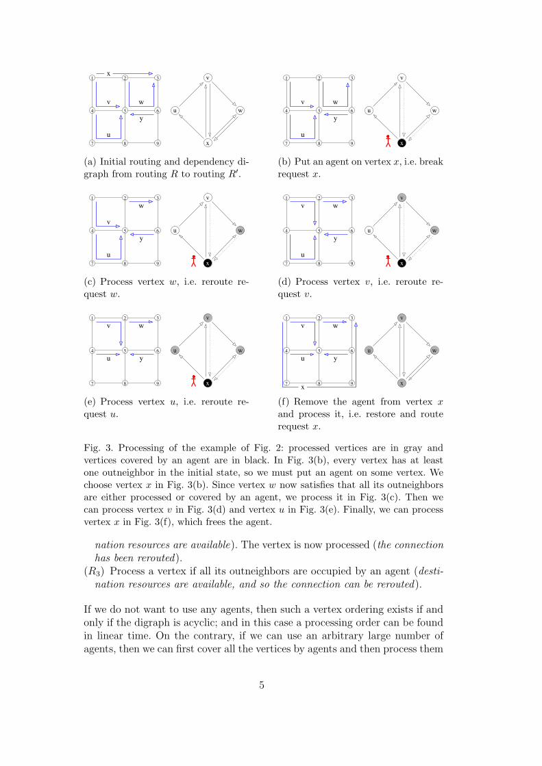
Fig. 3. Processing of the example of Fig. 2: processed vertices are in gray andvertices covered by an agent are in black. In Fig. 3(b), every vertex has at leastone outneighbor in the initial state, so we must put an agent on some vertex. Wechoose vertex x in Fig. 3(b). Since vertex w now satisfies that all its outneighborsare either processed or covered by an agent, we process it in Fig. 3(c). Then wecan process vertex v in Fig. 3(d) and vertex u in Fig. 3(e). Finally, we can processvertex x in Fig. 3(f), which frees the agent.

nation resources are available). The vertex is now processed (the connectionhas been rerouted).

(R3) Process a vertex if all its outneighbors are occupied by an agent (desti-nation resources are available, and so the connection can be rerouted).

If we do not want to use any agents, then such a vertex ordering exists if andonly if the digraph is acyclic; and in this case a processing order can be foundin linear time. On the contrary, if we can use an arbitrary large number ofagents, then we can first cover all the vertices by agents and then process them

5

in any order. We aim at minimizing the number of agents simultaneously inuse. The process number pn(D) of a digraph D is the minimum number ofagents for which there exits a process strategy for D. Notice that the processnumber is upper bounded by mfvs(D). A process strategy that uses p (atmost p, at least p, respectively) agents is a p-process strategy ((≤ p)-processstrategy, (≥ p)-process strategy, respectively).

The problem of determining the process number of a given dependency digraphhas been proved NP-complete and APX-complete [10]. In this paper, we focuson the problem of recognition and characterization of digraphs and graphswith small process numbers. We start in Section 2 by recalling some generalresults on the process number, its links with other graph invariant like the nodesearch number, and how to define it as a cops-and-robber games. Then, in Sec-tion 3, we first identify graphs with connectivity equal to the process number(Theorem 4). Then, we characterize graphs with process number at most 2in terms of excluded minors. Techniques used to this end are close to thatof Megiddo et al. [21], who gave the forbidden minors for graphs with searchnumber at most 2. We also provide a structural description (Theorem 9), fromwhich we design an algorithm to recognize (and, if possible, 2-process) suchgraphs in linear time in the number of edges (Subsection 3.1.2). We turn todigraphs in Section 4. We characterize digraphs with process number at most 2(Proposition 17), and show how to recognize whether a graph D has processnumber at most 2 (and if yes how to process it) in time O(n2(n + m)), wheren is the number of vertices of D, and m its number of arcs (Proposition 20).We conclude the paper in Section 5 with some open problems and directionsfor future works.

Let us give some notations before going further. The outneighborhood of X inD is

N+(X) := {v ∈ V : there exists u ∈ X such that (u, v) ∈ A} ,

The strict outneighborhood of X in D is

SN+D(X) := N+

D (X) \X .

The (strict) outneighborhood of a vertex x ∈ V is the (strict) outneighbor-hood of {x}, and the (strict) outneighborhood of a subgraph is the (strict) out-neighborhood of its vertex set. The inneighborhood of X is N−D (X) := N+

D′(X)where D′ is obtained from D by reversing the direction of every arc. In allthese notations, the subscript may be omitted if there is no risk of confusion.

6

2 General results on the process number

First, notice that the dependency digraph may contain loops. It may occurwhen the original and final routes of a lightpath use the same wavelength onthe same link of the network. In such cases, and depending on the specificitiesof the router nodes of the network, it is not always possible to establish thenew route before switching the lightpath. So a break-before-make might berequired.

Observation 1 Adding loops to the vertices of a digraph D increases theprocess number by at most 1.

PROOF. Consider a pn(D)-process strategy for D, let L be the order inwhich the vertices are processed, and let D∗ be the digraph obtained from Dby adding loops to each vertex. Since adding a loop to a vertex v forces tocover v by an agent before processing it, we can process D∗ following L usingat most one extra agent: it suffices to ensure that an agent is placed on avertex before processing it. So, pn(D∗) ≤ pn(D) + 1.

2

Let us note that the bound of Observation 1 cannot be further reduced ingeneral. For instance, the process number of a directed symmetric path (onat least 4 vertices) is 2, and adding a loop on each vertex yields a digraphwith process number 2. On the opposite, the process number of the digraph ofFigure 2(c) is 1 but adding a loop on w yields a digraph with process number 2.

It is straightforward to construct a loopless digraph D′ such that pn(D) =pn(D′), replacing each loop with a 2-cycle. Hence, unless stated otherwise, weconsider in the sequel loopless digraphs. When D is symmetric, we work forconvenience on the underlying undirected graph G = (V, E). So each undi-rected graph of this paper is to be seen as a symmetric digraph.

An important invariant for digraphs and graphs is the notion of vertex sepa-ration. Let D = (V, A) be a digraph and X a subset of its vertices. A layoutL of D is an ordering of the vertices, i.e. a one-to-one correspondence be-tween V and {1, 2, . . . , |V |}. The vertex separation of (D, L) is vsL(D), themaximum over all indices i ∈ {1, 2, . . . , |V |} of the size of the strict outneigh-borhood of {L−1(1), L−1(2), . . . , L−1(i)}. The vertex separation vs(D) of D isthe minimum, over all orderings L, of vsL(D). This notion naturally extendsto undirected graphs: the vertex separation of an undirected graph is the ver-tex separation of the corresponding symmetric digraph. Kinnersley [17] provedthat the vertex separation of any undirected graph equals its pathwidth, an

7

important invariant of graphs which was introduced by Robertson and Sey-mour [23].

The following result establishes a close link between the vertex separation andthe process number of a digraph. It was first proved by Coudert et al. [10],but we recall the proof here for completeness.

Proposition 2 ([10]) For every digraph D, vs(D) ≤ pn(D) ≤ vs(D) + 1.

PROOF. Consider a p-process strategy for D, and let L be the order inwhich the vertices are processed. Observe that if the strategy is stopped justafter the ith vertex has been processed, then any non-processed vertex havinga processed inneighbor must be covered by an agent. As this is true for everyi ∈ {1, 2, . . . , |V |}, this exactly means that the vertex separation of (D, L) isp, so vs(D) ≤ pn(D).

Let L be an ordering of the vertices of D, and let vsL(D) be the vertex sep-aration of (D, L). We consider the process strategy for D that consists ofprocessing the vertices in the increasing order induced by L. At any time, letP be the set of processed vertices and let M be the set of vertices covered byan agent. At each step, we ensure that M equals the strict outneighborhoodof P in D.

The first vertex can be processed by covering its at most vsL(D) neighbors byan agent. Suppose that i ≥ 1 vertices have been processed, and let v be thenext vertex to be processed. If v /∈M , then as the vertex separation of (D, L) isvsL(D) we infer that |M∪(N+(v)\P )| ≤ vsL(D). So we can put an agent overall the outneighbors of v that are not in M∪P and process v. This uses at mostvsL(D) agents simultaneously. If v ∈M , then |M\{v}∪(N+(v)\P )| ≤ vsL(D).Thus, putting an agent over all the outneighbors of v not in M∪P uses at most,and possibly, vsL(D) + 1 agents simultaneously. Hence, pn(D) ≤ vsL(D) + 1.

2

As determining the vertex separation of an arbitrary graph is APX-complete [12],the preceding result shows that the process number problem also is.

The pathwidth of a graph is also its node-search number, and is closely relatedto other graph-searching invariants [5, 27]. Indeed, the processed number inundirected graphs can be defined in terms of cops-and-robber games in whicha team of agents aims to catch an invisible and infinitely fast fugitive. Themain difference with the node search number is that with the process number,a vertex can be processed if all its neighbors are covered by an agent. Conse-quently, the fugitive is catched not only when it occupies the same vertex than

8

an agent, but also when it is surrounded by agents. Furthermore, a processstrategy is by definition a monotone game. Further study of the links betweenthe process number, the vertex separation and also the search number hasbeen performed recently [10, 26]. We refer the reader to the recent survey ofFomin and Thilikos about graph-searching [13].

The next proposition characterizes the optimal process-strategies for digraphswhose process number is different from their vertex separation.

Proposition 3 For any digraph D, there exists a pn(D)-process strategy suchthat each vertex is covered by an agent before being processed if and only ifpn(D) = vs(D) + 1.

PROOF. Suppose that the digraph D has a pn(D)-process strategy such thateach vertex is covered by an agent before being processed. Let v1, v2, . . . , vn bean enumeration of the vertices of D in the order in which they are processed.For each i ∈ {1, 2, . . . , n}, we set Xi := {v1, v2, . . . , vi}. Stop the strategy justbefore the vertex vi is processed. All the vertices in the strict outneighborhoodof Xi must be covered by agents, and so is also vi. Therefore, | SN+(Xi)| ≤pn(D) − 1 for each i ∈ {1, 2, . . . , n}, and hence vs(D) ≤ pn(D) − 1. So,vs(D) = pn(D)− 1 by Proposition 2.

Conversely, suppose that pn(D) = vs(D) + 1. Let H be the digraph obtainedfrom D by adding a loop to each vertex that does not have one already.Thus, any strategy that processes H must cover each vertex by an agentbefore processing it. Moreover, vs(H) = vs(D) and pn(D) ≤ pn(H). Sincepn(H) ≤ vs(H)+1 by Proposition 2, we infer that pn(H) = pn(D). Therefore,any pn(D)-strategy for H is a pn(D)-strategy for D that covers each vertexby an agent before processing it, as wanted. 2

3 Symmetric digraphs

Recall that for convenience, we work on the underlying undirected graphs ofsymmetric digraphs. Given an undirected graph G = (V, E), the neighborhoodNG(v) of a vertex v ∈ V is the set of all the vertices adjacent to v in G. Westart by characterizing graphs the connectivity of which equals the processnumber.

Theorem 4 A p-connected graph G can be p-processed if and only if thereexists a vertex v of degree p such that G−N(v) is an independent set.

9

PROOF. Let G be a p-connected graph. If there is a set of p vertices of Gthe deletion of which induces an independent set, then G has process numberat most p (and hence exactly p since the minimum degree of G is at least p).

Conversely, let G be a p-connected graph with pn(G) = p and consider a p-process strategy for G. Stop the strategy just before processing the first vertexv. Thus, all the neighbors of v are covered by agents. By the p-connectivity,G has minimum degree p. Consequently, v has degree exactly p. Let X be theset of vertices the neighborhood of which is contained in N(v) — and hence isexactly N(v), by the p-connectivity. Without loss of generality, we can assumethat the first steps of the strategy consist in processing all the vertices of X.If all the vertices not in N(v) have been processed, then the set N(v) fulfillsthe desired condition.

Otherwise, there exists a vertex w /∈ X ∪N(v). Define z to be the next vertexto be processed. Since the strategy uses p agents and all the vertices of X havealready been processed, we deduce that z ∈ N(v). Moreover, N(z) ⊂ X∪N(v).Thus, N(X ∪ {z}) ⊆ X ∪ N(v). Consequently, N(v) \ {z} is a set of p − 1vertices the deletion of which disconnects w from A ∪ {z}; a contradiction. 2

The class of graphs with process number at most p is closed under the oper-ation of taking minors. Indeed, assume that there exists a p-process strategyfor a given graph G. Let G′ be the minor of G obtained by contracting theedge uv into a single vertex w. Without loss of generality, suppose that u isprocessed before v — hence v is covered by an agent when u is processed.Apply the strategy to G′. The first step concerning the vertices u, v is to coverone of them by an agent. Instead, put an agent on w. The remaining of thestrategy can then be applied, ignoring the processing of u, and processing winstead of v. Thus, G′ also has process number at most p. We formalize thisas an observation.

Observation 5 Let G be a graph and H a minor of G. Then pn(G) ≥ pn(H).

We focus on graphs with small process number. The first interesting case iswhen p is 2, since only independent sets can be 0-processed and only the starshave process number exactly 1. We note here that Bodlaender proved thatevery minor-closed class of graphs that does not contain all planar graphs hasa linear time recognition algorithm [6]. This result follows from a linear timealgorithm that determines whether a graph has treewidth, or pathwidth, atmost k, and if so finds a tree decomposition, or a path decomposition, of widthat most k, respectively. However, this algorithm is rather impracticable [24].

10

(a) K4 (b) H0 (c) H1 (d) H2 (e) C5

Fig. 4. Some minor-obstructions for 2-processed graphs.

3.1 Graphs with process number 2

In this section, we characterize graphs with process number at most 2. Aspointed out in the introduction, Megiddo et al. [21] gave the list of forbiddenminors for graphs with search number at most 2. We use similar techniques.Nevertheless, graphs with process number at most 2 can have search number 3,and hence some extra work is needed to find the list of forbidden minors inour case. Next, we derive from the characterization an algorithm to recognizeand process such graphs, which is linear (in the number of nodes an edges) intime and space.

3.1.1 Characterization of graphs with process number 2

We start by exhibiting two families M1 and M2 of graphs (15 graphs in total)with process number greater than 2. We then prove that a graph has processnumber at most 2 if and only if none of its minors is in M1 ∪ M2. This isobtained via a structural characterization of those graphs. The next lemmafollows from Observations 5 and a straightforward checking.

Lemma 6 Let J be one of the graphs of Fig. 4. Every graph with a J-minorhas process number at least 3.

We now give a technical lemma, which is a direct analog of a lemma forpathwidth. We do not state it in full generality, since we only need the followingparticular case.

Lemma 7 Let G be a graph and v a vertex of G. If G− v has (at least) threeconnected components with process number p then pn(G) > p.

PROOF. Suppose on the contrary that pn(G) = p, and consider a p-processstrategy of G. For convenience Let J1, J2 and J3 be three components of G−veach of process number p. Observe that if an agent covers a vertex of Ji + v,then there is at least one vertex of Ji + v covered by an agent until the lastvertex of Ji + v is processed.

Up to relabelling the components, we may assume that Ji is the i-th compo-nents among J1, J2, J3 to have p of its vertices covered by agents (each of them

11

(a) Ta (b) Tb (c) Tc

(d) T1 (e) T2

Fig. 5. T1 and T2 are two of the ten non-isomorphic minor-obstructions for2-processed graphs obtained using three subgraphs chosen among Ta, Tb and Tc

and merged at vertex .

must reach such a state since pn(Ji) = p). Stop the strategy when p vertices ofJ2 are covered by agents. Then, no vertex of J1 is covered by an agent, whichimplies that all the vertices of J1 are processed (by our choice of the orderingof the components Ji and the remark above). Consequently, either a vertexof J3 + v is covered by an agent, or all the vertices of J3 are processed. Theformer is impossible since we consider a p-process strategy of G, and so is thelatter by our ordering of the components Ji. This contradiction concludes theproof. 2

Our next lemma exhibits another family of graphs with process number greaterthan 2. It directly follows from Observation 5 and Lemma 7.

Lemma 8 Let J consist of three graphs J1, J2, J3 chosen among Ta, Tb, Tc andmerged at vertex (see Fig. 5). Every graph with a J-minor has processnumber at least 3.

Let M1 be the collection of graphs depicted in Fig. 4 and let M2 be thecollection of graphs defined in Fig. 5. We observe that if a graph G has acut-vertex v such that at least three components of G− v are not stars, thenG necessarily contains a minor in M2. This is true because a connected graphthat is not a star contains either a cycle, or a path on at least four vertices.This observation is used several times in the sequel.

Given a vertex u of a graph G, a subgraph H of G− u is attached to u if thestrict outneighborhood of H in G is {u}. We can now give a complete char-acterization of graphs that can be 2-processed. Statement (c) of the followingtheorem is illustrated in Fig. 6.

Theorem 9 For every connected graph G = (V, E), the following assertionsare equivalent.

(a) pn(G) ≤ 2;(b) No minor of G is in M1 ∪M2;

12

u1 u2

u4

S14

u6

z17

z47S2

4

u3

z14

Fig. 6. A typical graph with process number 2.

(c) The following holds:· V = U ∪ Z ∪ T with U = {u1, . . . , ur} and Z = {zj

i : 1 ≤ i ≤ r and 1 ≤j ≤ ki} where k1, . . . , kr are non-negative integers;· each connected component of G[T ] is a star S`

i , for some ` ∈ N andi ∈ {1, 2, . . . , r}, which is attached in G to the vertex ui of U ;· each vertex zj

i ∈ Z has degree 2 in G, and its two neighbors are ui andui+1; and· N(ui) ∩ U ⊆ {ui−1, ui+1}, and if ki = 0 then ui+1 ∈ N(ui).

PROOF. The fact that (a) implies (b) follows from Lemmas 6 and 8. Let usshow now that (b) implies (c).

We prove the assertion by induction on the number of vertices of G, the resultbeing true if G has at most 3 vertices.

Suppose first that G is 2-connected. Thus, G contains a cycle of length 3 or 4,because it has no C5-minor. If G contains a 3-cycle C, then there exists avertex w not in C adjacent to at least two vertices of C, and exactly twosince G has no K4-minor. Let u and u′ be those two vertices, and let v bethe third vertex of C. Since G contains no H1-minor, the vertices v and whave degree 2 in G. Therefore, G consists of the edge uu′ and some vertices ofdegree 2 adjacent to both u and u′, and hence G fulfills condition (c). Assumenow that G has no 3-cycle, hence G has an induced 4-cycle C. If G is a 4-cycle,then the conclusion follows, so let us assume that w is a vertex of G not inC. We can moreover assume that w has at least 2-neighbors in C because Gis 2-connected. Since G has no 3-cycle, w has exactly 2 neighbors in C, whichare not adjacent. So w cannot have degree more than 2 in G, for otherwiseG would contain an H0-minor. Consequently, G consists of a 4-cycle uvu′v′

and some vertices of degree 2 adjacent to both u and u′, and hence G satisfiescondition (c).

We assume now that G has a cut-vertex w. Let X1, X2, . . . Xb be the connectedcomponents of G−w, and for each index i set Di := Xi + w. (Note that b ≥ 2since w is a cut-vertex.) If each Xi is a star, then setting r := 1 and u1 := w

13

shows that G satisfies (c). So we assume that X1 is not a star. As observedearlier, at most two components Xi may not be stars since no minor of G isin M1 ∪M2.

We assume first that only X1 is not a star. By the induction hypothesis, D1

fulfills condition (c), so we let U ′ := {u′1, u′2, . . . , u′s}, Z ′ and T ′ be as stated incondition (c). Observe that we can moreover assume that each vertex u′i with1 < i < s is a cut-vertex of D1 such that exactly two components of D1 − u′iare not stars. In particular, for i ∈ {1, s} the vertex u′i has a neighbor not inU ′ ∪ Z ′. We now consider several cases regarding whether w ∈ U ′, w ∈ Z ′ orw ∈ T ′.

If w ∈ U ′ then the graph G fulfills condition (c), the components X2, . . . , Xn

being just additional stars attached to w.

Second, suppose that w ∈ Z ′, and let u′i and u′i+1 be the two neighbours ofw in D1. Notice that one of u′i and u′i+1 has degree 2 in G, for otherwise Gwould contain H1 or H2 as a minor. By symmetry, we may assume that u′i+1

has degree 2. As a result, if u′iu′i+1 is an edge then i + 1 = s. Hence, setting

U := (U ′ \ {u′s}) ∪ {w} and Z := (Z ′ \ {w}) ∪ {u′s} shows that G fulfills thecondition (c). On the other hand, if u′i and u′i+1 are not adjacent, then since X1

is a connected component of G−w there exists a vertex z′i 6= w of degree 2 thatis adjacent to both u′i and u′i+1. Notice that there is only one such vertex, forotherwise G would have an H1-minor. Furthermore, since G does not containH0 as a minor, we deduce that u′i has degree 2 in G. Consequently, X1 is astar on 3 vertices, a contradiction.

Finally, assume that w ∈ T ′. So, w belongs to a star S ′ attached to u′i forsome i ∈ {1, . . . , s}. Suppose that w cannot be considered as the center of S ′.Then, by our assumption on U ′ and because no minor of G is in M2, we inferthat i ∈ {1, s}, say i = 1. Next, there exists a vertex of S ′−w that is adjacentto u1, since w is not a cut-vertex of D1. As a consequence, wu′1 is not an edgeof G, for otherwise H0 or H2 would be a minor of G. Let w′ be the center ofS ′. Setting U := U ′ ∪ {w, w′} yields the desired conclusion. If w is the centerof S ′, then a similar argument (with w = w′) applies if i ∈ {1, s}. So, supposethat 1 < i < s. In this case, the subgraph induced by ∪j>2Di is a star sinceno minor of G is in M2. Thus, G has the asserted structure.

It remains to deal with the case where another component Xi, say X2, is not astar. We assert that there exists a decomposition of D1 as in the condition (c),with the extra-condition that w is the vertex u1 of U . This would yield thesought result, since then the same applies to D2 (by symmetry), and hencesetting U := U ∪U ′, Z := Z ∪Z ′ and T := T ′ ∪ T ′′ would show that G fulfillsthe condition (c), as wanted.

14

To see that the assertion holds, we consider a decomposition (U ′, Z ′, T ′) ofD1 as in the previous case, i.e. U ′ := {u′1, . . . , u′s}, Z ′ and T ′ are as givenby condition (c) applied to the graph D1. We make the same assumption onU ′, i.e. every vertex u′i with 1 < i < s is a cut-vertex of D1 and exactly twocomponents of D1 − u′i are not stars.

It follows that if w ∈ U ′ then w = u′i with i ∈ {1, s}, since every vertex u′jwith 1 < j < s is a cut-vertex of D1. So we now assume that w /∈ U ′.

We assert that w /∈ Z ′. To see this, suppose on the contrary that w ∈ Z ′ andlet u′i and u′i+1 be the two neighbors of w in D1. Since w is not a cut-vertexof D1, we deduce that H2 is a minor of D1, and hence of G; a contradiction.

Consequently, w belongs to a star S ′ attached to a vertex u′i of U ′. We inferthat i ∈ {1, s} by condition (b), for otherwise u′i would be a cut-vertex of Gsuch that three connected components of G−u′i are not stars; a contradiction.By symmetry, say that i = 1. If w is a center of S ′, then we set u0 := w. Thisyields the sought decomposition of D1: the vertices of S ′ adjacent only to ware stars attached to it, and those adjacent to both w and u1 become verticeszj1. And if w cannot be considered as the center of S ′, then let w′ be the center

of S ′. As previously, we know that there is a vertex of S − w adjacent to u1.Therefore, w cannot be adjacent to u1. Thus, setting u0 := w′ and u−1 := wyields the sought decomposition of D1.

It remains to show that (c) implies (a). The graph G can be 2-processed asfollows. (1) Cover u1 by an agent and set i := 1; (2) While i < r: process allstars S`

i (this uses a second agent, which is freed at the end), cover ui+1 by anagent, process all vertices zj

i , process the vertex ui (which frees an agent) andincrement i; (3) Process ur. 2

Theorem 9 directly implies the following corollary.

Corollary 10 Given two graphs H and H ′ that can be 2-processed and theircorresponding vertices u1, u2, . . . , ur for H and u′1, u

′2, . . . , u

′s for H ′, the graph

G built from the union of H and H ′ and where the vertices ur and u′1 aremerged can be 2-processed.

3.1.2 An algorithm to recognize graphs with process number at most 2

We present a linear (in the number of nodes and edges) time and space com-plexity algorithm for deciding whether a graph can be 2-processed. We usethe notations of Theorem 9. The idea of the algorithm is as follows. First, wenote that we can decide whether a graph is a star in time O(|N(v)|+ |N(w)|),where v is any vertex of that graph and w ∈ N(v), since one of them mustbe a center of the star. Then, if we are given the vertex u1 of condition (c)

15

of Theorem 9, we can process all attached stars in time linear in their size,next identify the vertex u2, and so process the whole graph. Also, startingfrom vertex ui and thanks to Corollary 10, we can identify in linear time thevertex u1. Thus, the core of the algorithm is, starting from any vertex v, toidentify in linear time a vertex ui, which is done using a proper analysis of thesizes of the neighborhood at distance 1 and the neighborhood at distance 2 ofv.

Before going into details, we need some more ground work. We show thatdeciding whether a graph can be 2-processed can be done in linear time. Tothis end, we first note in Proposition 11 that we can decide very efficiently if agraph can be 1-processed, and in Proposition 12 that we can decide in lineartime if a 2-connected graph can be 2-processed.

From now on, we assume that a vertex v of G contains the list N(v) of itsneighbors, its degree, a Boolean variable v.active set to false if the vertexis covered by an agent or if it has been processed, and an integer — or apointer — v.tag, which is set to w if the vertex v is visited while processingthe vertex w. We also assume that we can access any vertex of G in constanttime, and finally that nei(v, w) is a function that returns in constant time 1if v ∈ N(w) and 0 otherwise. More precisely, the function nei uses an arrayof size |V (G)| initialized to 0. Neighbors of v are set to 1 at the beginningof the processing phase and set back to 0 at the end of the processing phasewhich can thus be done in time O(|N(v)|). So, the overall cost due to themanagement of nei for all the vertices ui (see Theorem 9) is linear in the sizeof G.

Proposition 11 Given a graph G and a vertex v, we can decide in timeO (|N(v)|+ |N(w)|) if G can be 1-processed or not, where w is any neighborof v.

PROOF. Since a star has at most one vertex of degree greater than 1, it issufficient to check that:

• if |N(v)| > 1, then every neighbor of v has degree 1. This can be checked intime O (|N(v)|);• if |N(v)| = 1, then the unique neighbor w of v cannot have neighbors of

degree greater than 1, which can be checked in time O (|N(w)|).

So, overall, the time complexity is O (|N(v)|+ |N(w)|). 2

Proposition 12 Given a 2-connected graph G, we can decide in linear timeif G can be 2-processed.

16

PROOF. Let n ≥ 3 be the order of G. By Theorem 4, a graph with no-cutvertex can be 2-processed if and only if it is either K2,n−2 or K2,n−2 plusan edge joining the two vertices of the bipartition of size 2.

Now, checking that G is one of the two graphs mentionned is done as follows.We choose three arbitrary vertices of G. One of them must have degree 2 andwe call u1 and u2 its neighbors. Now it remains to check that the neighborhoodof each vertex v ∈ V \ {u1, u2} is exactly {u1, u2}. This procedure is linear intime. 2

Proposition 13 Given a graph G, we can check in linear time if pn(G) ≤ 2.

PROOF. The proof consists of three steps. We use the notation of the asser-tion (c) of Theorem 9.

(1) First, we prove that if we are given a graph G and a vertex w, then wecan decide in linear time if G can be 2-processed under the constraint that wis the vertex u1 of the assertion (c) of Theorem 9. To this end, let us analyzethe algorithm described at the end of the proof of Theorem 9. We set u1 := w,and we suppose that we are at step i ≥ 1 of the loop. Recall that non-activevertices are ignored.

• Cover the vertex ui by an agent: We just have to set the Boolean variableui.active to false.• Remove from G all subgraphs of kind S`

i : First, we have to determine whichneighbors of ui belong to the stars S`

i and which belong to U or Z. Accordingto Proposition 11 we can decide whether a neighbor v of ui belongs toa star or not in time O (|N(v)|+ |N(u)|), where u is a neighbor of v, ifany. Note that we consider the degree of v and u minus nei(ui, v) andnei(ui, u), respectively. Simultaneously, we place a tag on all neighbors ofv and u, to avoid double checking. If v belongs to a star, we process it intime O (|N(v)|+ |N(u)|), setting the Boolean variables active to false. Soedges of stars will be visited twice during the processing of ui. We also visitall edges incident to ui+1 once.• Determine the vertex ui+1 and process all vertices zj

i : To determine ui+1, wehave to check that all remaining active neighbors of ui of degree 1 (i.e., ver-tices zj

i , if any) have the same neighbor, which should also be the remainingneighbor of degree greater than 1. (Note that there is such a neighbor forotherwise the previous step would have processed all the neighbors of w.)Then it remains to process the vertices zj

i . To this end, we first cover ui+1

by an agent. During this step, we visit all the remaining neighbors of ui

once.• Process the vertex ui, which frees an agent.

A graph G satisfies the assertion (c) of Theorem 9 with the vertex w being the

17

vertex u1 if and only if this algorithm processes the whole graph. Note thatthe algorithm fails if more than one vertex is a candidate to be the vertexui+1.

Overall, each edge of G is visited twice and a constant number of operationsare performed for each vertex. So we can process G in linear time.

(2) According to the previous step and Corollary 10, given a graph G and avertex ui, we can check in linear time if G can be 2-processed or not. Indeed,we process all subgraphs of G attached to ui that can be 1-processed. Now,if G− ui has more than two components, then G cannot be 2-processed, andthe algorithm returns false. If G − ui has no connected components, thenpn(G) ≤ 2; while if it has only one connected component H, then we applystep (1) on H+ui with w = ui. Otherwise, let H and H ′ be the two componentsof G− ui. We set J := H + ui and J ′ := H ′ + ui. Let UJ = {uJ

1 , . . . , uJt } and

UJ ′= {uJ ′

1 , . . . , uJ ′t′ } be the vertices given by Theorem 9(c) applied to J and

J ′, respectively.

As observed in the proof of Theorem 9, the graph G has process number atmost 2 if and only if J and J ′ both satisfy the assertion (c) of Theorem 9 withui being considered as the vertex uJ

1 and the vertex uJ ′1 . Thus, we apply step

(1) on J with uJ1 = ui. If step (1) succeeds then we apply step (1) on J ′ with

uJ ′1 = ui. Then G can be 2-processed if and only if this last step succeeds.

(3) It remains to find a vertex ui in G. We explain now a procedure thatreturns a vertex which can safely be considered as one of the vertices ui,provided that G fulfills condition (c) of Theorem 9. To this end, choose thevertex w of maximum degree of G. If vertex w has degree 2, then G is eithera path or a cycle and step (2) will give a correct answer with ui := w. If|N(w)| > 2, then w is either the center of a star or a vertex ui. Notice that thevertices of degree greater than 2 of G are contained in U ∪ T . Moreover, theyinduce a forest, each tree of the forest being a path of order at least 1 with anarbitrary number of vertices adjacent to precisely one vertex of the path. Inparticular, w is at distance at most 2 of one of the vertices ui. For i ∈ {1, 2},let ki be the number of vertices of degree at least 3 that are at distance i ofw. Let xi be such a vertex, for i ∈ {1, 2}, if any. The following follows fromour observations.

• If k1 + k2 = 0, then the procedure can safely return ui = w.• If k1 = 1, then (at least) one of w or x1 can safely be returned as being

a vertex ui. So, it is sufficient to check if the subgraph containing x1 inG− {w} is a star. If it is true, then the procedure returns w and otherwisex1.• The case where k1 = 0 and k2 = 1 is similar to the previous one, with x2

18

playing the role of x1.• If k1 ≥ 2, then w can be considered to be a vertex ui.• if k1 = 0 and k2 ≥ 2 then again w can be considered as a vertex ui.

To sum-up, we can find in linear time a vertex of U , which allows us to checkin linear time if G can be 2-processed. This concludes the proof. 2

A precise description of an algorithm to recognize graphs with process num-ber 2 (and obtain a 2-process strategy, if any) is given by Algorithms 1, 2, 3,4 and 5.

Algorithm 1 Function Test-2-process-from

Require: a connected graph G and a vertex u covered by an agent.Ensure: returns succeed if the graph G can be 2-processed with first covering

u by an agent.1: w.active← false

2: CC2 ← false {CC2 indicates if a connected component that cannot be1-processed has already been found.}

3: for all v ∈ N(u) such that v.active and v.tag 6= u do4: if Is-Star(G, v, u, u) then5: Process-Star(G, v, u)6: else if not CC2 then7: CC2 ← true

8: else9: return failed

10: if not CC2 then11: return succeed

12: FC ← false {FC indicates if we have found a candidate for the nextvertex to be visited, ui+1}

13: for all v ∈ N(u) such that v.active do14: if not FC then15: if |N(v)| = 2 then16: u′ ← N(v)− {u}17: else18: u′ ← v19: FC ← true

20: else if (|N(v)| = 2 and N(v)− {u} 6= {u′}) or (|N(v)| > 2 and v 6= u′)then

21: return failed

22: u.active← false

23: return Test-2-process-from(G, u′)

19

Algorithm 2 Function Is-Star

Require: a graph G, a vertex w that should belong to a star, a vertex u thatshould not be considered in the neighborhoods, and a tag t.

Ensure: returns true if w belong to a star and false otherwise. All visitedvertices receive tag t.

1: c← w2: if |N(u)| − nei(u, w) = 1 then3: c← N(w)− {u}4: c.tag← u5: bool← true

6: for all v ∈ N(c)− {u} do7: if |N(v)| − nei(u, v) > 1 then8: bool← false

9: v.tag← t10: return bool

Algorithm 3 Procedure Process-Star

Require: a graph G, a vertex w that belongs to a star and a vertex u thatshould not be considered in the neighborhoods.

Ensure: Inactivate all vertices of the star attached to w except u.1: c← w2: if |N(u)| − nei(u, w) = 1 then3: c← N(w)− {u}4: for all v ∈ N(c)− {u} do5: v.active← false

4 Digraphs

In this section we characterize the classes of directed graphs with processnumber at most 2. We start with some preliminary remarks.

A digraph can be 0-processed if and only if it has no cycles, that is if it isa dag. In particular a direct path can be 0-processed. Using a Depth FirstSearch [8], one can check in linear time whether a digraph is acyclic.

Lemma 14 For any digraph D, the process number of D is equal to the max-imum of the process numbers of its strongly connected components.

PROOF. Let dag-C be the acyclic digraph of the strongly connected com-ponents of D, i.e. each vertex of dag-C corresponds to a strongly connectedcomponent of D, and there is an arc from a vertex u to a vertex v if and onlyif there is an arc between the corresponding strongly connected componentsin D. We can process each strongly connected component of D separately, inthe order induced by dag-C. 2

20

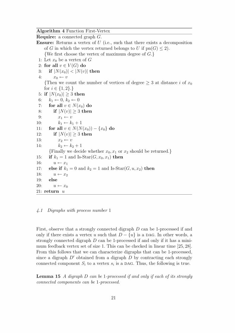
Algorithm 4 Function First-Vertex

Require: a connected graph G.Ensure: Returns a vertex of U (i.e., such that there exists a decomposition

of G in which the vertex returned belongs to U if pn(G) ≤ 2).{We first choose the vertex of maximum degree of G.}

1: Let x0 be a vertex of G2: for all v ∈ V (G) do3: if |N(x0)| < |N(v)| then4: x0 ← v{Then we count the number of vertices of degree ≥ 3 at distance i of x0

for i ∈ {1, 2}.}5: if |N(x0)| ≥ 3 then6: k1 ← 0, k2 ← 07: for all v ∈ N(x0) do8: if |N(v)| ≥ 3 then9: x1 ← v

10: k1 ← k1 + 111: for all v ∈ N(N(x0))− {x0} do12: if |N(v)| ≥ 3 then13: x2 ← v14: k2 ← k2 + 1

{Finally we decide whether x0, x1 or x2 should be returned.}15: if k1 = 1 and Is-Star(G, x0, x1) then16: u← x1

17: else if k1 = 0 and k2 = 1 and Is-Star(G, u, x2) then18: u← x2

19: else20: u← x0

21: return u

4.1 Digraphs with process number 1

First, observe that a strongly connected digraph D can be 1-processed if andonly if there exists a vertex u such that D − {u} is a dag. In other words, astrongly connected digraph D can be 1-processed if and only if it has a mini-mum feedback vertex set of size 1. This can be checked in linear time [25, 28].From this follows that we can characterize digraphs that can be 1-processed,since a digraph D′ obtained from a digraph D by contracting each stronglyconnected component Si to a vertex si is a dag. Thus, the following is true.

Lemma 15 A digraph D can be 1-processed if and only if each of its stronglyconnected components can be 1-processed.

21

Algorithm 5 Main procedure to 2-process graphs

Require: a graph G.Ensure: returns true if G can be 2-processed and false otherwise.1: w ← First-Vertex(G)2: Initialize nei to 0 and set neighbors of w to 1 O(n)3: w.active← false, bool← false, tag← 04: for all v ∈ N(w) such that v.active and v.tag 6= w do5: if Is-Star(G, v, w, tag) then6: Process-Star(G, v, w)7: else8: tag← tag + 19: if tag > 0 and tag < 3 then

10: for all v ∈ N(w) such that v.tag = 1 do11: v.active← false

12: x← v13: w.active← true

14: bool← Test-2-process-from(G, w)15: if tag = 2 and bool and x.tag = 1 then16: for all v ∈ N(w) such that v.tag = 1 do17: v.active← true

18: w.active← true

19: bool← Test-2-process-from(G, w)20: return bool

Forthwith a simple algorithm that decides in linear time and space complex-ity if a digraph can be 1-processed. This algorithm is an alternative to thealgorithms of Shamir [28] and Rosen [25], which better fits our setting. Inparticular, it can compute the minimum feedback vertex set of 1-processeddigraphs in linear time.

Proposition 16 Given a digraph D with n vertices and m arcs, decidingwether D can be 1-processed can be done in time and space complexity O(n +m).

PROOF. We assume in this proof that D is a strongly connected digraph.Otherwise, we identify each strongly connected component in time O(n + m)using a Depth First Search (dfs) and next we apply the following algorithm oneach stronlgy connected component without changing the overall complexity.

We use the observation that a strongly connected digraph D has process num-ber 1 if and only if there is a vertex v such that D− v is a dag. The followingshows how to determine whether such a vertex exists, and find one if any, intime O(n + m).

22

Since D is strongly connected, it contains a directed cycle C := x1x2 . . . xkx1

and so the vertex v must be one of the vertices xi. We maintain a list L ofvertices that are candidates to be the vertex v. To this end, we define L to bean array of k integers, initialized to 0. A vertex xi of C is valid if L[i] is 0.

Suppose that there exists a directed path xiy1y2 . . . y`xj with V (C) disjointfrom {y1, y2, . . . , y`}, for some non-negative integer `. (If ` = 0, then it meansthat there is an arc from xi to xj.) If i < j then none of the vertices xi+1, xi+2, . . . , xj−1

can be the sought vertex v. If j < i then none of the vertices xi+1, . . . , xk, x1, . . . , xj−1

can be the sought vertex v.

For i from 1 to k, we run a dfs rooted at xi and in which we do consider neitherthe outneighbors of the vertices of V (C) \ {xi}, nor the outneighbors of thevertices already visited during a previous dfs. For each vertex, we record thestep in which it is first visited, i.e., we record i if the vertex was first visitedduring the dfs rooted at xi. Consider the step i ∈ {1, 2, . . . , k}.

If the dfs reaches a vertex xj, then we set L[`] := i for each ` from j−1 downto i + 1 (modulo k). Note that if j = i, then it means that only xi remainsvalid, and so we can directly set v := xi and returns true if and only if D−xi

is a dag.

If xi is still valid and the dfs reaches a vertex already visited during, say, stepj < i, then we set L[`] := i for ` from j down to 1 and from k down to i + 1.

To cope with the complexity requirement, we make the vertices not valid ina backward way and stop when a vertex that has been removed previously isfound. So doing, each cell of L is modified once, and we test in total at mostO(m) times if a vertex is still valid. So the cost due to maintaining the list ofvalid candidates during the algorithm is O(n + m).

Observe that if a vertex xi ∈ V (C) is still valid once all the dfs are performed,then all the directed cycles of D that intersect C contain xi. Thus, if L isnon-empty then it suffices to return true if and only if D − xi is a dag. If Lcontains no valid vertices, then we can conclude that for each i ∈ {1, 2, . . . , k},the digraph D − xi contains a directed cycle, and consequently D cannot be1-processed.

Overall this algorithm takes time O(n + m). First, we can find a cycle intime O(n), for example by choosing a starting vertex and moving to the firstneighbor until we reach a vertex that has already been visited. Second, wevisit each arc of D once during the dfs. So this part takes time O(m). Also,the total cost due to L is O(n+m). Finally, we can check whether a subgraphof D is a dag in time O(n + m) using a dfs.

23

w’H’

Y’ Y

H

w

(a) General shape of a (2, w)-digraphw w’

Y’

YH

H’

(b) Example of a (2, w)-digraph

Fig. 7. The general shape and an example of a (2, w)-digraph.

The space complexity is linear since except the size of the graph, a dfs needsonly a stack, which can be implemented using an integer array of size n, andthe list of candidates uses an array of size at most n. 2

4.2 Digraphs with process number 2

Our aim in this subsection is to present a polynomial-time recognition algo-rithm for digraphs with process number 2.

Let D be a digraph and let w be one of its vertices. We say that D is a (2, w)-digraph if there exists an (≤ 2)-process strategy to process D, the first stepof which is to cover w by an agent. Thus, a digraph can be 2-processed if andonly if it is a (2, w)-digraph for some vertex w (see Fig. 7(b)). First, we showhow to determine efficiently whether D is a (2, w)-digraph for a given vertexw.

Proposition 17 Let D be a (weakly) connected digraph and let w be oneof its vertices. The digraph D is a (2, w)-digraph if and only if the digraphD−w can be partitioned into two subdigraphs H and H ′ satisfying the followingconditions:

(i) there exists a vertex w′ of H ′ such that H ′ is a (2, w′)-digraph;(ii) SN+

D(H + w) ⊆ {w′}(iii) either• pn(H) = 0; or• pn(H) = 1 and there exists a (possibly empty) set Y ⊂ V (H) such that

N−D ({w′})∩V (H) ⊆ Y , pn(D[Y ]) = 0, and (Y, V (H) \Y ) is a directedcut of H from Y to V (H) \ Y .

PROOF. If w has no outneighbors, then D is a (2, w)-digraph if and only ifpn(D − w) ≤ 2. So the characterization is valid with H being empty and H ′

being D − w. We assume now that w has at least one outneighbor in D.

24

Suppose that there exist two subdigraphs H and H ′ as in the statement of theproposition. The following strategy shows that D is a (2, w)-digraph. Coverw by an agent. If pn(H) = 0, then cover w′ by an agent, process H and thenprocess w by condition (ii). If pn(H) = 1, then set Y ′ := V (H) \ Y andprocess D[Y ′]. As SN+

D(Y ′) ⊆ {w} by the definition of Y ′ and by condition(ii), we use at most one more agent during this processing, and only w is stillcovered by an agent once D[Y ′] is processed. Now, cover w′ by an agent andprocess the vertices of Y , since SN+

D(Y ) ⊆ Y ′ ∪ {w, w′} by condition (ii) andpn(D[Y ]) = 0. Hence, in both cases, we have processed H, and w and w′ arecovered by agents. By condition (ii), we can now process w and then finish toprocess D since H ′ is a (2, w′)-digraph by condition (i).

Conversely, assume that D is a (2, w)-digraph, and consider a correspondingstrategy to process it. Note that at most one outneighbor of w is processedafter w, since the first step of the strategy consists in covering w by an agent.Stop the strategy just before w is processed. We let H be the subdigraph ofD induced by all the vertices processed before w, and H ′ be the complementof H in D−w. By the definition, |N+

D (H + w)∩V (H ′)| ≤ 1. If |N+D (H + w)∩

V (H ′)| = 0 then we define w′ to be the first vertex of H ′ to be covered by anagent according to the strategy, and otherwise we define w′ to be the uniqueoutneighbor of H+w in H ′. In this case, the vertex w′ must be already coveredby an agent. As the strategy uses no more than two agents simultaneously,there are no arcs from H + w to H ′ − w′, and so condition (ii) is fulfilled.

Recall that we consider the strategy only from the first step up to the laststep before processing w. Observe that w is covered by agent during all thesteps considered, and if w′ is covered by an agent at some point, then itstays covered until the last step considered. Consequently, no vertex of X :=N−D ({w′}) ∩ V (H) can be covered by an agent at any step considered, andhence pn(D[X]) = 0. It also follows from this observation that pn(H) ≤ 1. Ifpn(H) = 1, then we let vi be the i-th vertex of H to be covered by an agent(hence vi /∈ X). Let Y ′i be the outbranching of vi in H, that is

Y ′i := {h ∈ V (H) : there exists a directed path from vi to h in H} .

We set Y ′ := ∪iY′i . By the previous observation, we infer that Y ′ ∩ X = ∅.

Moreover, there are no arcs from Y ′ to Y := V (H)\Y ′. Finally, pn(D[Y ]) = 0.Thus, condition (iii) is fulfilled.

The remaining part of the strategy ensures that H ′ is a (2, w′)-digraph, asrequired by condition (i). 2

Before using the preceding characterization to derive a polynomial-time recog-nition algorithm, we state a useful lemma. Let D be a digraph and let w bea vertex of outdegree at most 1 of D. Let v be the unique outneighbor of w,if any. The contraction of w consists of removing w, linking every vertex of

25

Algorithm 6 Function Is-(2, w)-digraph

Require: a strongly connected digraph D and a vertex wEnsure: returns succeed if D is a (2, w)-digraph.1: Cover w by an agent and remove w from the neighborhoods of its prede-

cessors2: C ← set of strongly connected components of D − w3: Let dag-C be the dag of strongly connected components4: while it exists C ∈ C such that C is a leaf of dag-C and pn(C) ≤ 1 do5: Process C, and so remove it from D − w, C and dag-C{Let D1 be the remaining digraph}

6: D2 ← Contract-rooted(D1, w)7: if V (D2) = {w} then8: return succeed

9: else if |N+D2

(w)| = 1 then {we have N+D2

({w}) = {w′}}10: return Is-(2, w′)-digraph(D2 − w)11: else12: return failed

N−D (w) to v, and removing any parallel arcs created (but not the loops thatmay appear; we do so since parallel arcs are irrelevant regarding the processnumber, whereas — as noted in the introduction — loops are not).

Lemma 18 Let D be a digraph and w a vertex of D with exactly one outneigh-bor v. Let D′ be obtained by contracting w. Then pn(D) = pn(D′). Moreover,for every vertex u of D, it holds that D is a (2, u)-digraph if and only if D′ isa (2, u′) digraph with u′ = u if u 6= w and u′ = v otherwise.

PROOF. Consider a p-process strategy for D′. Apply it to D with the extrastep that w is processed as soon as v is processed or covered by an agent.This shows that pn(D) ≤ p. Conversely, consider a p-process strategy for D.Note that when w is processed then v is either already processed or coveredby an agent. We apply the strategy to D′, except that if a step covers w byan agent, we instead cover v (if it is not already covered, or processed). Thisyields a p-strategy for D′, since the remark above ensures that we do not useany extra agent in the strategy for D′.

The ’moreover’ part follows from above by a straightforward checking. 2

Proposition 19 Given a strongly-connected digraph D and a vertex w ∈V (D), Algorithm 6 decides in time O(n(n + m)) if D is a (2, w)-digraph.

PROOF. Let us prove that Algorithm 6 is correct. We assume that each timea vertex is processed, the neighborhoods of its predecessors are updated andso is the set V 1

D of vertices of out-degree at most 1.

26

Algorithm 7 Function Contract-rooted

Require: a connected digraph D and a vertex w of D.Ensure: returns a reduced digraph, but vertex w being unchanged.1: Let V 1

D be the set of vertices of D of outdegree at most 1.2: while V 1

D \ {w} is not empty do3: Let v be any vertex of V 1

D − {w}, which we remove from V 1D

4: if N+(v) > 0 then5: Let u′ be the outneighbor of v6: for all v′ ∈ N−(v) do7: N+(v′)← N+(v′) \ {v} ∪ {u′}8: if |N+(v′)| = 1 then9: V 1

D ← V 1D ∪ {v′}

Suppose first that D is a (2, w)-digraph. We consider the partition (H, H ′)of D − w and the subset Y ⊆ V (H) given by Proposition 17. We set Y ′ :=V (H) \ Y . If pn(H) = 0, then we may assume that Y = V (H), and henceY ′ = ∅.

Since pn(H) ≤ 1 and N+D (Y ′) ⊆ Y ′ (arcs to w are removed by line 1), lines 2–5

will remove the whole digraph D[Y ′], because (Y, Y ′) is a directed cut of H.Also, D[Y ] is a dag since pn(D[Y ]) = 0. Hence, every leaf vertex u of D[Y ]without an arc to w′ will be removed as {u} becomes a strong component onceD[Y ′] is removed. Let Y r ⊆ Y be the remaining part of Y . The digraph D[Y r]is a dag the leaf vertices of which have for unique outneighbor w′. Thus, line 6— and so Algorithm 7 — will contract every vertex of Y r into w′, startingfrom the leaf vertices. Note that H ′ = D2 − w.

Now, Algorithm 6 returns failed only if either the vertex w has more thanone outneighbor in H ′ = D2−w, or it has a unique outneighbor w′ in H ′ butH ′ is not a (2, w′)-digraph. None of these cases happens by Proposition 17.Therefore, Algorithm 6 returns succeed, as desired.

Conversely, suppose now that the algorithm returns succeed for a given di-graph D, and let us prove that D is a (2, w)-digraph. We start by coveringw by an agent. The algorithm starts by removing strongly-connected compo-nents that are leaves in dag-C, and have process number at most 1. We cansafely process all these components using at most one other agent, which isfreed at the end. Note that after these steps, the remaining digraph may notbe strongly connected anymore, but the vertex w has outdegree at least 1.Thanks to Lemma 18, we can ignore the contraction step of line 6. Then, asthe algorithm returns succeed, either only w remains, and we just process wto finish, or w has exactly one outneighbor called w′, and the digraph D2−wis a (2, w′)-digraph. Thus, we can cover w′ by an agent, process w and thenfinish to process D2−w using at most two agents simultaneously. This showsthat D is a (2, w)-digraph by Lemma 18.

27

The computation time of Algorithm 6 has two parts. The first part concernsthe partition into strongly connected components (line 2) that takes timeO(n+m), the construction of dag-C (line 3) in time O(n), the application oneach strongly-connected component of the algorithm of Proposition 16 for anoverall cost in O(n + m) including the update operations of line 5, and finallyat most n recursive calls (line 10). Overall this part takes time O(n(n + m)).

The second part concerns Algorithm 7 and the maintenance of the correspond-ing data structures. Since the computation time of line 7 depends on the datastructures chosen to store the digraph, we assume that the list of in- (respec-tively out-) neighbors is stored in an unsorted double linked list plus an arrayof size n recording for each neighbor its pointer in the list. Thus, we may addor remove a vertex of the in- (respectively out-) neighborhood of a vertex inconstant time. Since a vertex may be contracted only once, and since in theworst case it has O(n) predecessors, this part takes an overall time of O(n2).

Finally, the computation time of Algorithm 6 is in O(n(n + m)). 2

We note that Algorithm 7 can me modified to decide if a strongly connecteddigraph D can be 1-processed, since it would then be contracted into a singlevertex with a loop.

The process number of a digraph is at most p if and only if the process numberof each of its strong components is at most p. Indeed, suppose that each strongcomponent of a digraph D can be p-processed. The digraph D′ of the strongcomponents of D is acyclic. It suffices to p-process each strong component ofD according to a topological order of D′ to p-process D. Thus, we obtain thefollowing result thanks to Proposition 19.

Proposition 20 Given a digraph D we can decide in time O(n2(n + m)) ifit can be 2-processed.

5 Conclusion

We modeled a rerouting problem in wdm networks using graph theory. Tothis end, we introduced a new (di)graph invariant, the process number, whichturns out to be closely related to other well-studied invariants of (di)graphs. Inparticular, as Proposition 2 shows, it is a refinement of the vertex-separation(also called pathwidth in the case of undirected graphs). We also characterizedthe (optimal) process strategies of digraphs the process number of which isdifferent from their vertex separation (Proposition 3).

Our next goal was to characterize and recognize efficiently (di)graphs with

28

small process number. In particular, we gave a linear time algorithm forrecognition of graphs with process number at most two (Proposition 13, Al-gorithm 1), as well as a characterization in terms of excluded minors and astructural description (Theorem 9). For digraphs with process number two,we found a characterization that allows to recognize (and process) them intime O(n2(n+m)). Finally, we linked the process number to the connectivity,by determining the graphs with process number equal to their connectivity(Theorem 4).

As for the excluded minor characterization, we are currently studying [11]graphs with process number 3. It may be the last case achievable, since wehave so far a list of 185 266 forbidden minors, which are highly structured. Itis interesting to note that for the pathwidth, such a characterization has beenfound up to pathwidth three [18] — for which there are 110 forbidden minors.On the other hand, the list for pathwidth 4 is not known, but it containsat least 122 millions forbidden minors and hence is probably out of reach.By Proposition 2, determining the excluded minors for graphs with processnumber 3 can be viewed as a scaling of this last problem, in the sense thatthis class contains graphs with pathwidth 3 and graphs with pathwidth 4.

Finally, we point out that heuristic have recently been designed to approximatethe process number [9]. It would be interesting to further study this aspect ofthe question.

References

[1] M. Ackroyd, Call repacking in connecting networks, IEEE Transactions onCommunications 27 (3) (1979) 589–591.

[2] D. Banerjee, B. Mukherjee, Wavelength-routed optical networks: Linearformulation, resource budgeting tradeoffs, and a reconfiguration study,IEEE/ACM Transactions on Networking 8 (5) (2000) 598–607.

[3] S. Beker, D. Kofman, N. Puech, Offline MPLS layout design and reconfiguration:Reducing complexity under dynamic traffic conditions, in: InternationalNetwork Optimization Conference (INOC), 2003.

[4] S. Beker, N. Puech, V. Friderikos, A tabu search heuristic for the off-lineMPLS reduced complexity layout design problem, in: IFIP-TC6 NetworkingConference (Networking), vol. 3042 of Lecture Notes in Computer Science,Springer, Athens, Greece, 2004.

[5] D. Bienstock, N. Robertson, P. Seymour, R. Thomas, Quickly excluding a forest,Journal of Combinatorial Theory, Series B 52 (2) (1991) 274–283.

[6] H. L. Bodlaender, A linear-time algorithm for finding tree-decompositions ofsmall treewidth, SIAM Journal on Computing 25 (6) (1996) 1305–1317.

29

[7] X. Chu, T. Bu, X.-Y. Li, A study of lightpath rerouting schemes in wavelength-routed WDM networks, in: IEEE International Conference on Communications(ICC), IEEE, Hong-Kong, 2007.

[8] T. Cormen, C. Leiserson, R. Rivest, Introduction to Algorithms, The MIT Press,1990.

[9] D. Coudert, F. Huc, D. Mazauric, N. Nisse, J.-S. Sereni, Reconfiguration of therouting in WDM networks with two classes of services, in: 13th Conferenceon Optical Network Design and Modeling (ONDM), IEEE, Braunschweig,Germany, 2009.

[10] D. Coudert, S. Perennes, Q.-C. Pham, J.-S. Sereni, Rerouting requestsin wdm networks, in: Septiemes Rencontres Francophones sur les AspectsAlgorithmiques des Telecommunications (AlgoTel’05), Presqu’ıle de Giens,2005.

[11] D. Coudert, J.-S. Sereni, Obstruction set for graphs with process number three,in preparation.

[12] N. Deo, S. Krishnamoorthy, M. A. Langston, Exact and approximate solutionsfor the gate matrix layout problem, IEEE Transactions on Computer-AidedDesign 6 (1987) 79–84.

[13] F. V. Fomin, D. M. Thilikos, An annotated bibliography on guaranteed graphsearching, Theoretical Computer Science 399 (3) (2008) 236–245.

[14] M. Garey, D. Johnson, Computers and Intractability: A Guide to the theory ofNP-completeness, Freeman NY, 1979.

[15] N. Jose, A. Somani, Connection rerouting/network reconfiguration, in: 4thInternational Workshop on Design of Reliable Communication Networks(DRCN), IEEE, Banff, Alberta, Canada, 2003.

[16] B. G. Jozsa, M. Makai, On the solution of reroute sequence planning problemin MPLS networks, Computer Networks 42 (2) (2003) 199 – 210.

[17] N. G. Kinnersley, The vertex separation number of a graph equals its pathwidth,Information Processing Letters 42 (6) (1992) 345–350.

[18] N. G. Kinnersley, M. A. Langston, Obstruction set isolation for the gate matrixlayout problem, Discrete Applied Mathematics 54 (2-3) (1994) 169–213.

[19] O. Klopfenstein, Rerouting tunnels for MPLS network resource optimization,European Journal of Operational Research 188 (1) (2008) 293 – 312.

[20] K.-C. Lee, V. Li, A wavelength rerouting algorithm in wide-area all-opticalnetworks, IEEE/OSA Journal of Lightwave Technology.

[21] N. Megiddo, S. L. Hakimi, M. R. Garey, D. S. Johnson, C. H. Papadimitriou,The complexity of searching a graph, J. Assoc. Comput. Mach. 35 (1) (1988)18–44.

30

[22] G. Mohan, C. Murthy, A time optimal wavelength rerouting algorithmfor dynamic traffic in WDM networks, IEEE/OSA Journal of LightwaveTechnology 17 (3) (1999) 406–417.

[23] N. Robertson, P. D. Seymour, Graph minors. I. Excluding a forest, Journal ofCombinatorial Theory, Series B 35 (1) (1983) 39–61.

[24] H. Rohrig, Tree decomposition: A feasibility study, Master’s thesis, Max-Planck-Institut fur Informatik, Germany (1998).

[25] B. Rosen, Robust linear algorithms for cutsets, Journal of Algorithms 3 (3)(1982) 205–217.

[26] J.-S. Sereni, Colorations de graphes et applications, Ph.D. thesis, Ecoledoctorale STIC, Universite de Nice-Sophia Antipolis (July 2006).

[27] P. D. Seymour, R. Thomas, Graph searching and a min-max theorem for tree-width, Journal of Combinatorial Theory, Series B 58 (1) (1993) 22–33.

[28] A. Shamir, A linear time algorithm for finding minimum cutsets in reduciblegraphs, SIAM Journal on Computing 8 (4) (1979) 645–655.

[29] E. Wong, A. Chan, T.-S. Yum, A taxonomy of rerouting in circuit-switchednetworks, IEEE Communications Magazine 37 (11) (1999) 116–122.

[30] E. Wong, A. Chan, T.-S. Yum, Analysis of rerouting in circuit-switchednetworks, IEEE/ACM Transactions on Networking 8 (3) (2000) 419–427.

[31] J. Y. Zhang, O. W. W. Yang, J. Wu, M. Savoie, Optimization of semi-dynamiclightpath rearrangements in a wdm network, IEEE Journal on Selected Areasin Communications 25 (9) (2007) 3–17.

31