CHAPTER TWO

Causes and Consequences of RegionalVariations in Health Care1

Jonathan SkinnerDepartment of Economics, Dartmouth College, Hanover, NH, USA

Contents

1. Introduction 462. An Economic Model of Regional Variations in Health Care 48

2.1. The Demand Side 492.2. The Supply Side 502.3. A Typology of Health Care Services 54

3. Empirical Evidence on Geographic Variations in Expenditures and Utilization 573.1. Units of Measurement and Spatial Correlations 573.2. Health Care Expenditures 59

3.2.1. Adjusting for Prices 593.2.2. Adjusting for Differences in Health Status 623.2.3. Adjusting for Income 643.2.4. Regional Variation in Non-Medicare Expenditures 65

3.3. Effective Care (Category I) 663.4. Preference-sensitive Treatments with Heterogeneous Benefits (Category II) 673.5. Supply-sensitive (Category III) Treatments with Unknown or Marginal Benefits 71

4. Estimating the Consequences of Regional Variation: Geography As An Instrument 755. Inefficiency and the Policy Implications of Regional Variations 816. Regional Variations in Health Outcomes 837. Discussion and Conclusion 85References 86

Abstract

There are widespread differences in health care spending and utilization across regions of the US aswell as in other countries. Are these variations caused by demand-side factors such as patient prefer-ences, health status, income, or access? Or are they caused by supply-side factors such as providerfinancial incentives, beliefs, ability, or practice norms? In this chapter, I first consider regional healthcare differences in the context of a simple demand and supply model, and then focus on the empiri-cal evidence documenting causes of variations. While demand factors are important—health in

1 This chapter was written for the Handbook of Health Economics (Vol. 2). My greatest debt is to John E. Wennberg for

introducing me to the study of regional variations. I am also grateful to Handbook authors Elliott Fisher, Joseph

Newhouse, Douglas Staiger, Amitabh Chandra, and especially Mark Pauly for insightful comments, and to the

National Institute on Aging (PO1 AG19783) for financial support.

45Handbook of Health Economics, Volume 2ISSN: 1574-0064, DOI: 10.1016/B978-0-444-53592-4.00002-5

© 2012 Elsevier B.V.All rights reserved.

particular—there remains strong evidence for supply-driven differences in utilization. I then considerevidence on the causal impact of spending on outcomes, and conclude that it is less important howmuch money is spent, and far more important how the money is spent—whether for highly effectivetreatments such as beta blockers or anti-retroviral treatments for AIDS patients, or ineffective treat-ments such as feeding tubes for advanced dementia patients.

Keywords: health economics; health care productivity; spatial models; regional variations; small-areaanalysis

JEL Codes: I100; I110; I120; I180; R120

1. INTRODUCTION

A recently published Atlas documented dramatic differences in the utilization of

an important health input. Relative to the rates observed in the Boston area, utiliza-

tion was 74 percent higher in New Haven and more than 200 percent higher in San

Francisco.2 One might explain differences in utilization by variations in income,

health status, or prices, yet these factors do not appear to explain away the wide varia-

tions we observe. So why have these patterns—in per capita consumption of meat and

poultry, ranging from 31 pounds in the Boston region to 113 pounds per capita in the

San Francisco region—not received more attention from health experts or health

economists?

In this chapter, I attempt to distinguish between the admittedly puzzling geo-

graphic variation in meat and poultry consumption and geographic variation in health

care utilization. There are certainly many reasons why regional variations in utilization

can be justified by underlying health status, preferences and income, or productivity

differences among providers—surgical rates should be higher in regions where sur-

geons get better results (Chandra and Staiger, 2007). But there are also reasons why

such variations might not be efficient. We know that specific components of the

health care industry, such as the widespread use of insurance with modest co-

payments, leads to the twin problems of moral hazard and adverse selection. And

beginning with Arrow (1963), economists have argued that many of the unique fea-

tures and institutions associated with medical care—ranging from not-for-profit own-

ership to licensure of providers to the structure of insurance—are best understood as

the result of “uncertainty in the incidence of disease and in the efficacy of treatment”

(Arrow, 1963, p. 941).

2 http://maps.ers.usda.gov/FoodAtlas/

46 Jonathan Skinner

Health care is not the only sector of the economy with these characteristics—car

repair, home construction, and management consultancies exhibit uncertainty about

the efficacy of the fix, even if they are not typically insured to the same degree. While

regional variations surely exist in the quality and cost of automotive repairs, it is less

likely that the government would propose accountable car repair organizations, for

example.

Regional variations in health care are different, for at least two reasons. First,

assuming that the variation we observe is “unwarranted” in the sense that it cannot be

explained by legitimate causes such as health status, the magnitude of variation is so

large that the potential gain from erasing such inefficiencies—3 percent of GDP or

more in the United States—is worth pursuing. And second, these inefficiencies are

unlikely to be shaken out by normal competitive forces, given the patchwork of pro-

viders, consumers, and third-party payers each of which faces inadequate incentives to

improve quality or lower costs (Fuchs and Milstein, 2011).

Following on the earlier survey by Charles Phelps in the Handbook (Phelps,

2000), this review considers five general questions in reflecting on the economics

of regional variations in health care. First, what are the theoretical causes of such dif-

ferences? Traditionally, the presence of regional variation in medical care utilization

has been viewed through the lens of “supplier-induced demand,” the idea that

regional variations can be explained by the utility-maximizing behavior of health

care providers responding to a fee-for-service environment and relative scarcity (or

abundance) of providers (McGuire, 2011). The problem arises when individual

physicians in two seemingly similar regions—with identical insurance mechanisms

and similar patients—end up providing much different quantities of health care.

That is, standard supplier-induced demand models may argue that physicians do

more for their patients than is optimal, but does not typically explain why physi-

cians in McAllen, TX, do so much more for their Medicare patients than those in

El Paso (Gawande, 2009). To address these issues, I adopt a model based on

Chandra and Skinner (2011) and Wennberg et al. (2002) to parse out both supply

and demand factors that might be expected to explain regional variation in specific

types of treatment, ranging from highly effective care that clearly saves lives at min-

imal cost (such as beta blockers for heart attack patients) to very expensive treat-

ment without known benefits for patients (like proton beam therapy for prostate

cancer).

Second, I use this basic framework to consider the empirical evidence on causes of

geographic variation in health care utilization and expenditures. This is the key sec-

tion to assess the evidence on whether supply-side variations really do exist. If all of

the regional variation in observed utilization rates can be explained by other factors

such as patient preferences, relative prices, income, and health, then the puzzle of

regional variations is not even a puzzle any more. I focus in this chapter largely on

47Causes and Consequences of Regional Variations in Health Care

US regional variations, but document also a growing literature reflecting international

variations both within and across countries.3

Third, what are the consequences of higher health care spending? Does more spending

yield better outcomes—or is how the money spent more important for health? A key

focus of this section is to understand how geography might be used as a statistical instru-

ment in health economics to help estimate whether greater intensity of care is associated

with better health outcomes. Starting with the early work by Glover (1938) and

Wennberg and Gittelsohn (1973), and continuing through the more formal analysis

using instrumental variables, there has been a long-standing tradition of using geography

as an instrument to make inferences about the health care “production function”(Fisher

et al., 2003b; McClellan et al., 1994). Some studies have suggested a negative association

between spending and outcomes, while others have found a positive association, but

what is most striking is how much variability there is in outcomes across providers or

regions, and how poorly such variability is associated with factor inputs.

Fourth, what are the policy implications of observing variations in health care uti-

lization? If there are enormous variations in the productivity of concrete, a seven-digit

SIC code output with readily apparent quality measures (Syverson, 2004), is it any

surprise that there are even greater disparities in the productivity of health care across

regions or hospitals where outputs are difficult to measure and rarely made public?

The sometimes slow diffusion of valuable and highly efficient medical innovations, as

in Phelps (2000), has strong parallels with the slow diffusion of knowledge observed

across countries (Eaton and Kortum, 1999; Skinner and Staiger, 2009), yet the practi-

cal challenges of how to “fix” such slow diffusion rates across regions (or countries)

are still being debated.

Finally, while there are regional variations in health care utilization, there are also

strong gradients across the US in health (Kulkarni et al., 2011), and the two appear

only incidentally correlated (Fuchs, 1998). Explaining variations in health is perhaps

even more important, and suggests a greater focus on factors other than medical care

that may have a more direct impact on health, such as regional variation in the per

capita consumption of beef and poultry.

2. AN ECONOMIC MODEL OF REGIONAL VARIATIONSIN HEALTH CARE

Economic models typically include a demand and supply side, and so I adopt a

simple model from Chandra and Skinner (2011) to characterize each side of the

market.

3 For a useful bibliography of such studies, see WIC (2011).

48 Jonathan Skinner

2.1. The Demand SideThe demand side, based on Hall and Jones (2007) and Murphy and Topel (2006), is a

simplified two-period model of consumption and leisure where the individual’s per-

ceived quality of life, s(x), is in turn influenced by medical spending x:

V 5UðC1Þ1sðxÞUðC2Þ11 δ

ð2:1Þ

where Ci is consumption in period i, δ is the discount rate, and x measures health

care inputs.

Assume the expected survival or quality of life function is concave, so that s0(x)$ 0,

sv, 0. The Grossman model includes a variety of different approaches that individuals may

improve their health “stock” but in this simplified model the demand for health is expressed

solely through the demand for x (Grossman, 1972). Utility is maximized subject to the

budget constraint:

Y1 1Y2

11 r2P5C11 px1

C2

11 rð2:2Þ

where Yi is income or transfer payments in period i, p the consumer price of health

care, P the premium (or tax) paid for insurance, and r is the interest rate. Assume that

x is measured in units of what one dollar in real resources will purchase, meaning that

the true or social cost (q) per unit of x is normalized to one, but where the patient

pays p. (Thus if the coinsurance rate is 20 percent, p5 0.2.) This demand-side model

is straightforward, even if the assumptions implicit in this model can sometimes be at

odds with the empirical evidence.4

Maximizing the utility function (2.1) subject to (2.2), and rearranging yields the

optimality condition:

Ψ5UðC2Þ

ð11 δÞ @U@C1

5p

s0ðxÞ ð2:3Þ

Let Ψ be individual demand for an extra quality-adjusted year of survival, which

could in theory vary across regions for a variety of reasons: higher income, for exam-

ple, implies a lower marginal utility of first-period consumption and hence a much

higher demand for health care. Differences in the curvature of the utility function

4 For example, because demand is a function of the inverse of the marginal utility of first-period consumption, when

the Arrow�Pratt risk aversion parameter is 3 (or the intertemporal elasticity of substitution is 1/3), doubling

consumption increases demand and leads to 23 times the demand for health care (Murphy and Topel, 2006). As Hall

and Jones explain, the marginal utility of a third flat-screen TV falls rapidly relative to the demand for the ultimate

luxury good—health (Hall and Jones, 2007). Yet we do not typically observe such large income elasticities at a point

in time.

49Causes and Consequences of Regional Variations in Health Care

(and hence risk aversion) and the time preference rate can further affect the trade-off

between current consumption and future health.

2.2. The Supply SideI assume that physicians seek to maximize the perceived value of health for their

patient, given by Ψs(x), subject to financial considerations, resource capacity, ethical

judgment, and patient demand (Chandra and Skinner, 2011). While there are dishon-

est physicians that belie this assumption, it is at least consistent with the majority of

physician behavior. In this simple model, physicians act as price takers, but may still

face a wide array of different prices paid by private insurance, Medicare, and

Medicaid, for the identical procedure. This model therefore misses the complexity of

markets in which hospital groups and physicians jointly determine quantity, quality,

and price (Pauly, 1980).

Physicians also care about the income they make. For simplicity, let income be repre-

sented by R1πx, where R is the physician’s salary and π measures the net revenue aris-

ing from the procedure (or more generally, the vector of different procedures) x. Note

that the price paid by the patient, p, could be quite different from the profitability of the

procedure, π, and that when the provider is paid less than marginal cost, then π. 0, but

when the procedure is profitable, π, 0.

Thus the health care provider is assumed to maximize the sum Ψs(x)1Ω(R1 πx), where Ω is a function that captures the trade-off between the physician’s

desire to improve the value of patient survival and her own income. But the provider

may still be constrained by factors such as capacity constraints (a lack of available hos-

pital beds, so that x#X, where X is the local hospital bed supply) or ethical judgment

(the treatment is not worth the social cost or the patient is not better off as a conse-

quence when s0(x) is small or even negative and out-of-pocket expenses are high);

these additional restrictions are reflected in a portmanteau constraint μ.5 In this simpli-

fied case, the optimality condition for the provider can be written as

Ψs0ðxÞ52ωπ1 μ � λ ð2:4Þwhere ω is the derivative of Ω with respect to x, or the marginal value of an extra

dollar of income, and the combination of constraints is summarized by the shadow

price λ. For example, if financial incentives to do more (that is, 2ωπ, 0) are in turn

offset by ethical standards to “do no harm” to patients (μ5ωπ), so that λ5 0, then

physicians seeking to do the best for their patients would drive s0(x) to zero.

Consider Figure 2.1, showing both Ψs0(x) and λ.6 Note also the key assumption

that patients are sorted in order from most appropriate to least appropriate for

5 See Chandra and Skinner (2011) for a complete derivation of the model.6 Note that λ could vary with x; for simplicity it is held constant.

50 Jonathan Skinner

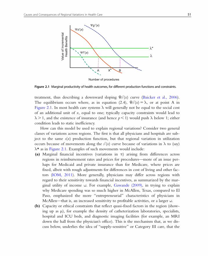
treatment, thus describing a downward sloping Ψs0(x) curve (Baicker et al., 2006).

The equilibrium occurs where, as in equation (2.4), Ψs0(x)5λ, or at point A in

Figure 2.1. In most health care systems λ will generally not be equal to the social cost

of an additional unit of x, equal to one; typically capacity constraints would lead to

λ. 1, and the existence of insurance (and hence p, 1) would push λ below 1; either

condition leads to static inefficiency.

How can this model be used to explain regional variations? Consider two general

classes of variations across regions. The first is that all physicians and hospitals are sub-

ject to the same s(x) production function, but that regional variation in utilization

occurs because of movements along the s0(x) curve because of variations in λ to (say)

λ* as in Figure 2.1. Examples of such movements would include:

(a) Marginal financial incentives (variations in π) arising from differences across

regions in reimbursement rates and prices for procedures—more of an issue per-

haps for Medicaid and private insurance than for Medicare, where prices are

fixed, albeit with rough adjustments for differences in cost of living and other fac-

tors (IOM, 2011). More generally, physicians may differ across regions with

regard to their sensitivity towards financial incentives, as summarized by the mar-

ginal utility of income ω. For example, Gawande (2009), in trying to explain

why Medicare spending was so much higher in McAllen, Texas, compared to El

Paso, emphasized the more “entrepreneurial” characteristics of physicians in

McAllen—that is, an increased sensitivity to profitable activities, or a larger ω.(b) Capacity or ethical constraints that reflect quasi-fixed factors in the region (show-

ing up as μ), for example the density of catheterization laboratories, specialists,

hospital and ICU beds, and diagnostic imaging facilities (for example, an MRI

down the hall from the physician’s office). This is the mechanism that, as we dis-

cuss below, underlies the idea of “supply-sensitive” or Category III care, that the

B

Ψg ′(x)

λV

alue

of I

ncre

men

tal

Hea

lth B

enef

its

Number of procedures

x*A

Ψs′(x)

λ*Ψf ′(x)

Figure 2.1 Marginal productivity of health outcomes, for different production functions and constraints.

51Causes and Consequences of Regional Variations in Health Care

shadow price of the extra bed-day is so low because there are empty beds.7

These differences in quasi-fixed capacity may in turn arise from historical acci-

dents; in contrast to New Haven, for example, there were a larger number of

religious groups establishing hospitals in Boston (Wennberg, 2010).

(c) Patient price or access. If most patients are uninsured and facing full dollar cost,

or if they tend to be wary of surgical procedures, then the physician is assumed

to account for their higher costs and avoid marginally valuable treatments.

Conversely, if it takes a long time for patients to get to the clinic or hospital, or

they face high implicit costs of doing so, then x will be lower (and s0(x) higher).(d) Malpractice risk, which changes the implicit costs or benefits of performing the

procedure. In some cases, “defensive medicine” can work to reduce λ and

increase utilization: the CT scan to provide cover for sending a patient home

from the emergency room or the PSA test to avoid lawsuits in the event that the

patient is later diagnosed with prostate cancer (King and Moulton, 2006). In

other cases, malpractice concerns may increase the implicit costs if by performing

the procedure the physician puts herself at greater risk of a lawsuit (Baicker et al.,

2007; Currie and MacLeod, 2008).

Recall that all these variations in capacity, financial incentives, and so forth would

lead to different points along the same production function. Thus if all regions were

on the same production function s(x), the cross-sectional association across regions

between spending and outcomes should trace out the production function and hence

the marginal “value” of health care spending. If regions also differ with regard to their

production function s(x), as is argued below, then these cross-regional comparisons

will no longer trace out s(x) over ranges of x, but some combination of both variation

in the production function and variation in λ. As I argue below, this creates difficultiesin interpreting regression coefficients seeking to answer the question “is more

better?”

A second approach to explaining geographic variations arises by allowing the pro-

duction function to differ across regions or physicians. Most obviously, this will occur

because of differences in health status; Lafayette, LA, has more underlying disease bur-

den than Hawaii, so we might expect the physician production function in Lafayette

to look more like f(x) than s(x) in Figure 2.1—there is most likely no amount of

health care spending that will make Lafayette as healthy as Hawaii. As well, one would

expect that for any given x, f 0(x). s0(x).A more interesting reason for variations in the production function—shifted from

s(x) to g(x) in Figure 2.1—is that physicians may have adopted more effective

7 This also begs the question of why a particular region might have so much capacity to begin with; capacity can best

be described as predetermined rather than exogenous. One study did find evidence that hospital beds are less likely

to move than people; thus regions subject to out-migration tend to have the greatest supply of beds (Clayton et al.,

2009).

52 Jonathan Skinner

innovations with small costs, such as checklists for surgeries or beta blockers for heart

attacks, thus enhancing the productivity of a given level of inputs x (de Vries et al.,

2010; Skinner and Staiger, 2009). Similarly, physicians may also be more skilled at a

specific procedure for people with similar health status. For example, in one study of

heart attack patients, patients experienced better outcomes from cardiac interventions

in regions with higher rates of surgery, consistent with a Roy model of labor market

sorting (Chandra and Staiger, 2007). Other explanations for such differences rely also

on systematically different organizational structures of practices (de Jong, 2008).

Physicians may also be overly optimistic (as in g0(x) in Figure 2.1) or pessimistic

( f 0(x)) about their ability in performing procedures, or more generally about the mar-

ginal effectiveness of specific treatments. For example, arthroscopic surgery to treat

osteoarthritis of the knee was a common procedure in the early 2000s, with 650,000

performed annually at a cost of about $5,000 each. In this procedure, surgeons enter

the joint area with tiny instruments, and clean out the joint while removing loose par-

ticles. In 2002, a randomized study of this procedure was conducted, with “sham”

surgery performed on the control group (Moseley et al., 2002). No benefit was found

relative to the control group, suggesting that, prior to the study’s publication, the per-

ceived surgical production function was to the right of the true production function

in Figure 2.1.

Alternatively, physicians may not understand that in treating a patient for a specific

disease, their prescription drug may interact with others already prescribed by other

providers (Zhang et al., 2010b), reflecting the problem that networks become increas-

ingly complex with more specialists involved (Becker and Murphy, 1992). In either

case, one can end up with different regions operating on different production func-

tions, with vastly different approaches to treatments, even though patients may not be

aware that they are receiving more or less intensive care (Fowler et al., 2008).

What about the interaction between supply and demand? After all, every one of the

650,000 patients annually undergoing arthroscopic knee surgery (prior to 2002) agreed

to the procedure, which even in the absence of out-of-pocket costs involved pain and

lost time for recovery. Presumably the patient formed beliefs of her marginal benefit in

part based on the physician’s expertise, and so the perceived demand for the procedure

would depend on physician advice. This is not “supplier-induced demand” per se; after

all, it is the physician’s job to convey expert information about the incremental benefits

of the procedure to the patient. But given the spectrum of opinions held by physicians

across regions (Sirovich et al., 2005), it should not be surprising if variations in physi-

cian opinions are mirrored by variations in patient beliefs across regions.

Less well understood is why patients sometimes appear to hold a more optimistic

view of the marginal benefits of treatment than even their physician. For example, the

COURAGE trials for patients with stable angina showed that stents, wire-mesh cylin-

drical devices inserted in narrowing cardiac arteries to improve blood flow, provided no

53Causes and Consequences of Regional Variations in Health Care

survival or heart-attack benefit to their patients, although it did reduce pain and improve

functioning modestly for several years (Boden et al., 2007). In a matched survey of

patients and physicians, physicians in one teaching hospital understood this evidence

from the COURAGE trial. By contrast, their patients believed, falsely, in the protective

effects of a stent against early death and heart attacks (Rothberg et al., 2010b).

Another way in which the traditional demand model falls short is where patients

are observed to use too little of high-value drugs such as anti-hypertensives, suggesting

an absurdly low value placed on their own life (Chandra et al., 2010). Indeed, even

when the monetary price is zero or even negative (Volpp et al., 2008), utilization of

effective treatments is below what it should be, raising questions of whether behav-

ioral models of demand are better descriptions of behavior. Still, it seems unlikely that

such anomalies in behavior should explain regional variations in demand.

In considering the empirical evidence, I will attempt to distinguish between the

λ-based variation, which may reflect both supply- and demand-side factors, and varia-

tions in actual or perceived production functions (or marginal productivity measures),

as has been found in other non-health care industries (Syverson, 2011).

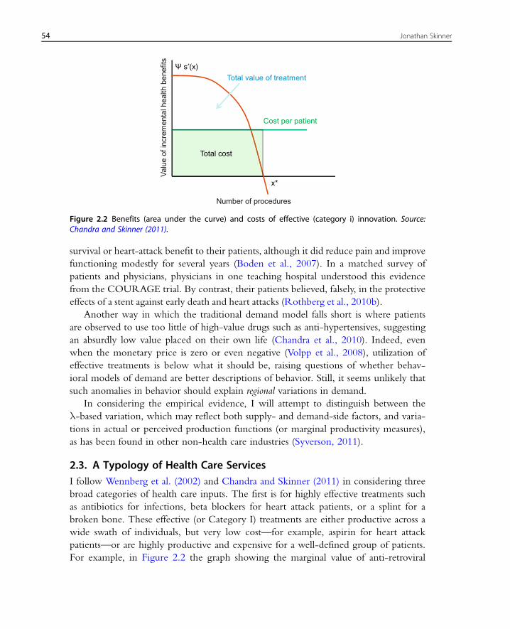
2.3. A Typology of Health Care ServicesI follow Wennberg et al. (2002) and Chandra and Skinner (2011) in considering three

broad categories of health care inputs. The first is for highly effective treatments such

as antibiotics for infections, beta blockers for heart attack patients, or a splint for a

broken bone. These effective (or Category I) treatments are either productive across a

wide swath of individuals, but very low cost—for example, aspirin for heart attack

patients—or are highly productive and expensive for a well-defined group of patients.

For example, in Figure 2.2 the graph showing the marginal value of anti-retroviral

Number of procedures

x*

Cost per patient

Total cost

Ψ s′(x)

Total value of treatment

Val

ue o

f inc

rem

enta

l hea

lth b

enef

its

Figure 2.2 Benefits (area under the curve) and costs of effective (category i) innovation. Source:Chandra and Skinner (2011).

54 Jonathan Skinner

treatments for HIV and AIDS patients. These are clearly beneficial (albeit very expen-

sive) for those with the disease. But even when s0(x) is driven to zero—that is, physi-

cians do not worry about the high price but only give the drug to patients who

would benefit—there is still little margin for overuse, because the side-effects are suffi-

ciently serious to preclude widespread usage. Thus net value, or the area under the

curve minus the cost (shown as the shaded rectangle in Figure 2.2), is still very large

(Chandra and Skinner, 2011).

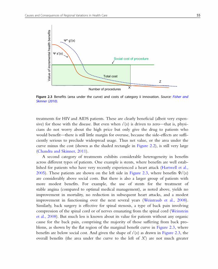
A second category of treatments exhibits considerable heterogeneity in benefits

across different types of patients. One example is stents, where benefits are well estab-

lished for patients who have very recently experienced a heart attack (Hartwell et al.,

2005). These patients are shown on the left side in Figure 2.3, where benefits Ψs0(x)are considerably above social costs. But there is also a larger group of patients with

more modest benefits. For example, the use of stents for the treatment of

stable angina (compared to optimal medical management), as noted above, yields no

improvement in mortality, no reduction in subsequent heart attacks, and a modest

improvement in functioning over the next several years (Weintraub et al., 2008).

Similarly, back surgery is effective for spinal stenosis, a type of back pain involving

compression of the spinal cord or of nerves emanating from the spinal cord (Weinstein

et al., 2008). But much less is known about its value for patients without any organic

cause for the back pain, comprising the majority of those suffering from back pro-

blems, as shown by the flat region of the marginal benefit curve in Figure 2.3, where

benefits are below social cost. And given the shape of s0(x) as drawn in Figure 2.3, the

overall benefits (the area under the curve to the left of X0) are not much greater

Val

ue o

f inc

rem

enta

l hea

lth b

enef

its

Number of procedures

Ψ s′(x)

Social cost of procedure

Total cost

X′

Ψ* g′(x)

Z

Figure 2.3 Benefits (area under the curve) and costs of category ii innovation. Source: Fisher andSkinner (2010).

55Causes and Consequences of Regional Variations in Health Care

than the overall costs, given by the rectangle to the left of X0 (Chandra and Skinner,

2011).

Figure 2.3 also shows that small changes in the marginal benefit curve could have

a strong impact on demand when the incremental medical value of the treatment is

small, at least relative to other options. For example, preferences could play an impor-

tant role in tonsillectomy rates, or choosing between mastectomy (removal of the

breast) and lumpectomy followed by radiation therapy for the treatment of breast can-

cer, given that the two options yield similar long-term prognosis. These preferences

would affect the perceived value of the treatment ( g0(x) versus s0(x) in Figure 2.3) or

differences in income or demand more generally (Ψ* versus Ψ) all could exert a large

influence on overall unconstrained utilization (Z versus X0 in Figure 2.3), particularly

at a point where out-of-pocket costs are low or non-existent and physicians are well

compensated for providing the treatment. To the extent that patient preferences, phy-

sician skills, or capacity constraints for these procedures might differ across regions, we

might expect to find large differences in utilization rates across otherwise similar

patients.

“Supply sensitive” or Category III variations are types of treatments where the evi-

dence either points to very small or zero effects, such as arthroscopy of the knee, or

where the benefits are simply not known. For example, there are a variety of treat-

ments for prostate cancer, with wide variations in costs but no clear evidence of supe-

riority for one type of treatment over another (Leonhardt, 2009). Category III

treatments also reflect the importance of available resources such as intensive care unit

(ICU) beds, hospital beds, specialists, and other “system”-level parameters, but where

there’s really no evidence on what is the right rate of ICU admissions among chroni-

cally ill patients. As noted above, capacity is reflected by variations in λ, but to the

extent that capacity is in turn determined by the perceived value of specific proce-

dures (e.g. g(x) versus s(x)), then capacity constraints become endogenous across

regions. Given the close association between overall Medicare expenditures and

Category III utilization rates (e.g. Wennberg et al., 2002), these types of utilization

are likely to play a large role in explaining overall spending differences across regions.

The next section provides a selected tour of the geographic variations literature in

light of this model, although the question addressed at each stage is: What is the

regional factor (and not simply idiosyncratic characteristics of physicians or patients)

that might be expected to explain geographic variation in expenditures? In other

words, it is not enough to find that (for example) physician practice varies dramatically

across individual physicians even after controlling for health status of the patient

(Phelps, 2000), since random variations among physicians would tend to cancel out

when averaged over very large numbers of physicians in New York or Los Angeles.

More interesting is what causes characteristics of patients and providers to be corre-

lated systematically within regions.

56 Jonathan Skinner

3. EMPIRICAL EVIDENCE ON GEOGRAPHIC VARIATIONS INEXPENDITURES AND UTILIZATION

By necessity, much of the evidence from the United States uses Medicare claims

data for the over-65 population, which is the closest insurance program to universal

health care in the US. Given that standard economic variables such as co-payment

rates and deductibles are the same across regions in the Medicare program, Medicare

utilization should in theory exhibit less variation than for the under-65 population

where characteristics of insurance plans—particularly Medicaid benefits—vary broadly

across the country. And while patterns from Medicare spending do not always gener-

alize to the under-65 population, the elderly do consume a disproportionate fraction

of health care spending, and growth in the Medicare program represents considerable

financial risk for the future stability of US government finances.

3.1. Units of Measurement and Spatial CorrelationsIn the early 1990s, the Dartmouth group sought to characterize regional markets in

preparation for what was supposed to have been Clinton-era health care reform. They

used 1992/93 discharge data from the Medicare population to determine “catchment

areas” for local hospitals, or “hospital service areas” (HSAs). There were 3,436 HSAs,

which in turn were combined to create 306 “hospital referral regions” (HRRs)

required to have at least one tertiary hospital providing cardiovascular and neurosurgi-

cal services. As in the 1973 Wennberg and Gittelsohn study, utilization was deter-

mined by residence (in this case zip code), and not by where the treatment was

actually received. Thus treatments received in Minneapolis by a resident of

Davenport, Iowa, would be assigned to the Davenport HRR, and not to

Minneapolis. The 306 HRRs did not generally follow county or state boundaries, but

instead reflected the actual migration patterns of Medicare patients, sometimes by fol-

lowing interstate highway routes. These definitions have not been changed since the

original Dartmouth Atlas, published in 1996 (Wennberg and Cooper, 1996), which

makes temporal comparisons straightforward, as the zip code-based crosswalks have

been modified over time to preserve the same geographical boundaries. The temporal

stability, however, means that regions may no longer be as sharply defined given secu-

lar changes in hospital market catchment areas.

Some studies have used state-level data, with the idea that some part of regional

variations may be explained by differences in state policies such as nursing home bed-

hold policies or Medicaid payments (Intrator et al., 2007). However, there is consider-

able variation within states, particularly large ones such as California, Texas, Florida,

or New York. Another approach is to use county-level data, which provides a much

larger sample of counties and the ability to match with other county data, for example

57Causes and Consequences of Regional Variations in Health Care

from the Center for Disease Control’s Behavioral Risk Factor Surveillance System

(BRFSS) data on health and health behaviors. Still, county boundaries may be imper-

fect aggregations of where people actually seek their care, particularly in rural areas

with small counties that do not have their own hospital.

An alternative is to create cohorts based on relative distance to specific hospitals,

such as a 10-mile circumference, or based on relative distance to specific types of hos-

pitals. For example, McClellan et al. (1994) considered heart attack patients living rel-

atively near to, or far from, a hospital with a catheterization laboratory used to

provide surgical treatment. Thus patient zip code was an instrument to predict

whether the individual received surgical intervention for their heart attack, with the

implicit assumption that unobservable health status was similar across zip codes.

Another approach is to avoid the use of zip codes altogether, but instead to create

“physician�hospital networks” or cohorts of individual patients based on where they

tend to seek care. For example, several studies created such networks using Medicare

claims data by first assigning patients to the primary care physician who sees them the

most, and then by assigning the physician to the hospital to which they are most loyal

(Bynum et al., 2007; Fisher et al., 2007). That is, the Princeton-Plainsboro physi-

cian�hospital network comprises patients who see the set of physicians who in turn

are most likely to admit to Princeton-Plainsboro, even if the patient has never been

admitted to that (or any) hospital.8 While these groups are no longer based on zip

codes, they do provide measures of costs and quality at a potentially relevant decision-

making unit, particularly for integrated delivery systems.

One key disadvantage of the Medicare claims data is the presence of Medicare-

sponsored managed care plans (Medicare Advantage). These are capitated plans by

which Medicare pays a fixed amount (adjusted by risk factors) to insurance companies

to provide coverage for their enrollees. As such, claims data are unavailable for this

group, yet in some regions of the country, roughly 40 percent are enrolled in

Medicare managed care. While there are concerns that the population in these plans

are systematically healthier than in the fee-for-service plans (Brown et al., 2011), there

is less evidence that selection issues have introduced bias in estimated measures for the

fee-for-service population, particularly when risk adjusters are specific to that same

population.9

Finally, a methodological shortcoming for most of this literature, particularly in

section 4, is the lack of accounting for spatial autocorrelation across regions. For

8 Nearly every Medicare enrollee sees at least one doctor annually, meaning that few enrollees are unassigned. These

networks are very similar to the structure of patient populations in “accountable care organizations” under the 2010

health care reform legislation in the US.9 One might be concerned that regions with rapid growth in Medicare Advantage would also experience above-

average growth in per-capita fee-for-service expenditures as healthier patients risk-select into Medicare Advantage.

However, unpublished data suggest that the change in Medicare Advantage enrollment across HRRs does not have

much predictive power in explaining growth in fee-for-service spending, as one might expect.

58 Jonathan Skinner

example, when researchers run a regression with 306 HRRs, they implicitly assume

independence; that the error term in the regression for Boston tells us nothing about

the error term for Worcester. But as Ricketts and colleagues have shown, this assump-

tion is demonstrably false (Ricketts and Holmes, 2007). Often, although not always,

adjusting for spatial autocorrelation leads to wider confidence intervals; thus studies

without such adjustments (including most of the Dartmouth studies) who find either

negative or positive influences of spending on outcomes could be falsely rejecting the

null of no effect.

3.2. Health Care ExpendituresDifferences in expenditures across regions provides a first look at variations, as well as

highlighting the magnitude of spending differences, at least in the Medicare claims

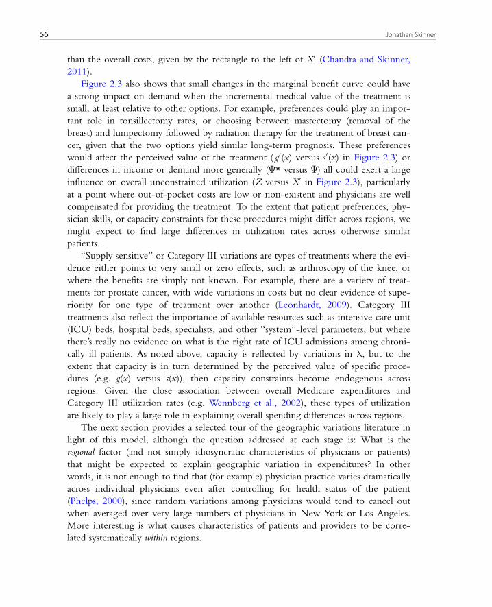
data. Table 2.1 shows a select group of regions along with a set of measures corre-

sponding to overall expenditures in Columns 1 and 2. Column 1 shows average per-

capita Medicare expenditures adjusted for age, sex, and race for 2007. There are

remarkable differences in expenditures across regions, from $6,196 in Grand Junction,

CO, to $16,316 in Miami, FL, with a coefficient of variation equal to 0.18.10 Indeed,

Miami is something of an outlier, having been at the top of the list for expenditures

per capita in every year since the Atlas began collecting data in 1992. The difference

in Medicare expenditures across regions is considerably larger in present value terms;

for Grand Junction versus Miami, the net difference in expected lifetime payout

approaches $100,000 assuming a 3 percent growth rate in real expenditures and a 3

percent discount rate. Thus Medicare redistributes substantial amounts of money

across regions—particularly as a fraction of a typical elderly person’s lifetime wealth

and income—even after controlling for income and taxes paid (Feenberg and Skinner,

2000).

3.2.1. Adjusting for PricesOne objection to comparing expenditures across regions is that Medicare pays more

per procedure in high-cost cities than in low-cost rural areas. When Medicare pays its

providers, it adjusts payments in several ways: (1) cost-of-living (using slightly different

approaches for hospital payments versus physician payments), (2) the disproportionate-

share program (DSH) which provides additional reimbursements for hospitals serving

low-income patients, and (3) providing additional reimbursements (per DRG) to com-

pensate for training medical and surgical residents. Following the earlier work by the

Medicare Payment Advisory Commission (MedPAC, 2009), Gottlieb et al. removed

these price differences by applying common national prices per diagnostic-related

10 The coefficient of variation reported in Table 2.1 is the ratio of the standard deviation to the mean, weighted by

the overall Medicare population in each region.

59Causes and Consequences of Regional Variations in Health Care

Table 2.1 Regional Variation in Utilization and Health: Selected MeasuresColumn/HRR 1 2 3 4 5 6 7 8 9

Year 2007MedicareExpenditures

2007MedicareExpenditures(priceadjusted)

2007MortalityRates(per1,000)

2005 HipFractures(per1,000)

1994/95 βBlockerUse (%)ideal pts

2007BackSurgery(per1,000)

2003PSATestsAge801(%)

2007End-of-Life ICUDays

2001�05Last 2 yrsMD Visits

Grand

Junction,

CO

6,196 6,283 4.58 7.47 5.9 9.0 1.4 38

Huntington,

WV

8,634 9,269 6.38 8.73 46 2.8 12.0 2.0 59

New York,

NY

12,190 9,691 4.37 6.30 61 2.0 27.0 4.0 88

Rochester, NY 6,613 6,923 5.50 6.99 82 3.4 5.3 2.1 45

Chicago, IL 10,369 9,782 4.70 6.70 36 2.5 13.7 7.4 81

San Francisco,

CA

8,498 6,881 4.25 5.45 65 3.1 13.4 4.6 64

Los Angeles,

CA

10,973 9,685 4.42 6.24 44 4.0 24.8 8.0 109

Seattle, WA 7,126 6,718 4.68 6.27 52 5.3 13.4 2.9 45

McAllen, TX 14,890 15,026 4.59 6.30 5 3.3 24.9 8.0 100

Miami, FL 16,316 15,971 4.96 7.27 52 2.5 30.4 10.7 106

Bend, OR 6,520 6,457 4.67 7.72 50 7.4 8.4 1.6 38

US average 8,571 8,571 5.04 7.34 51 4.5 19.0 3.9 61

Coefficient of

variation

0.18 0.16 0.09 0.14 0.27 0.31 0.35 0.43 0.32

Correlation

coefficient*

0.87 1.00 0.37 0.33 20.24 20.12 0.36 0.62 0.68

*With price adjusted per capita Medicare spending.Sources noted in text.

group (DRG) weight for inpatient care, and resource-value unit (RVU) for outpatient

care (Gottlieb et al., 2010). For other categories where quantity units were less appar-

ent, such as outpatient care, they applied a wage-index adjustment.

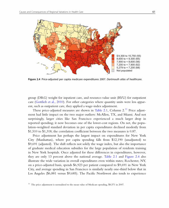
These price-adjusted measures are shown in Table 2.1, Column 2.11 Price adjust-

ment had little impact on the two major outliers: McAllen, TX, and Miami. And not

surprisingly, larger cities like San Francisco experienced a much larger drop in

reported spending; it now becomes one of the lower-cost regions. On net, the popu-

lation-weighted standard deviation in per capita expenditures declined modestly from

$1,510 to $1,318; the correlation coefficient between the two measures is 0.87.

Price adjustment has perhaps the largest impact on expenditures for New York

City (Manhattan), where per capita spending falls from $12,190 (unadjusted) to

$9,691 (adjusted). The shift reflects not solely the wage index, but also the importance

of graduate medical education subsidies for the large population of residents training

in New York hospitals. Once adjusted for these differences in expenditures, however,

they are only 13 percent above the national average. Table 2.1 and Figure 2.4 also

illustrate the wide variation in overall expenditures even within states; Rochester, NY,

on a price-adjusted basis, spends $6,923 per patient compared to $9,691 in New York

City, and average spending in San Francisco is similarly nearly one-third below that in

Los Angeles ($6,881 versus $9,685). The Pacific Northwest also tends to experience

$ 9,300 to 15,750 (55)8,600 to < 9,300 (65)7,900 to < 8,600 (56)7,200 to < 7,900 (62)5,279 to < 7,200 (68)Not populated

Figure 2.4 Price-adjusted per capita medicare expenditures 2007. Dartmouth atlas of healthcare.

11 The price adjustment is normalized to the mean value of Medicare spending, $8,571 in 2007.

61Causes and Consequences of Regional Variations in Health Care

lower spending levels, with Seattle ($6,178) and Bend, OR ($6,457), among the low-

est in the country.

3.2.2. Adjusting for Differences in Health StatusAn immediate concern with these comparisons of spending is that the standard

age�sex�race adjustment fails to adjust for health status. Bend, OR, may experience

low levels of spending, but this may in turn reflect a healthier population who main-

tain exercise and healthy diets after retirement. In the context of the model, regions

with poorer health status will experience greater incremental value of health care

spending, such as g0(x) compared to s0(x) in Figure 2.1, leading to appropriate spend-

ing differences across regions (for the same λ) given different production functions of

health, as shown by points A and B in Figure 2.1. Ideally, one would want to adjust

for differences across regions in illness burden to ask the question of whether there is

any regional variation left over that is not explained by health differences.

The most straightforward approach to risk adjustment is to consider mortality—a

reliably measured marker of illness, particularly since simply being in one’s last year of

life predicts elevated spending. Huntington, West Virginia, is distinguished by one of

the highest age�sex�race-adjusted Medicare mortality rates in the US: 6.32 percent

compared to a US average of 5.12 percent, as shown in Table 2.1, Column 3.12 Yet

overall expenditures in Huntington, WV, are just 8 percent above average ($9,269). Itmay be that the larger share of lower-income households in Huntington experience

worse access to care—fewer physicians in rural areas surrounding Huntington, for

example. However, income per se (independent of health status) does not appear to

explain regional variations in overall expenditures (Zuckerman et al., 2010), although

other factors, such as rural location and local poverty, could have a larger impact on

the supply of health care providers.

Note that mortality rates in the highest-expenditure regions, McAllen (4.47 per-

cent) and Miami (5.12 percent), are below the national average. One could interpret

this correlation in two ways. One is that these regions are in fact healthier than aver-

age, making their high level of health care spending all the more remarkable.13 But a

different interpretation reverses the causation: high spending in Miami and McAllen

leads to better health and hence lower mortality rates. Strictly speaking, one cannot

distinguish between these two hypotheses without estimating the causal effects of

spending, discussed in section 4 below.

12 These mortality estimates, from 2007, are for all Medicare enrollees, and not just those in the fee-for-service

population.13 Recall that residence is determined by the zip code from the Medicare denominator file corresponding to the

billing address. For snowbirds who travel back and forth between (say) McAllen and Rochester, NY, the billing

address could be in either locale, but health care expenditures would be a weighted average of health care received

in the two regions. Thus retirees would attenuate regional differences; McAllen’s spending would be lower and

Rochester’s higher because of this assignment rule.

62 Jonathan Skinner

An alternative health risk factor is the rate of hospital admissions for hip fractures.

Nearly every elderly person with a hip fracture is admitted to the hospital, and nearly

every doctor agrees on the clinical criteria for hip fractures. Furthermore, hip fractures

are largely determined by bone density, arising from early-life nutritional habits rather

than current environment or health care services (Lauderdale et al., 1998).

Huntington, WV, also experiences an elevated rate of hip fractures (8.73 per thou-

sand), higher than the US average (7.34). Miami (7.27) and McAllen (6.30) are lower

than average, with San Francisco among the lowest in the country (5.45). As discussed

in section 6, variations in health are large (the coefficient of variation for hip fractures

is 0.14), and not highly correlated with spending; the correlation coefficient between

hip fracture rates and price-adjusted expenditures is 0.33.

Yet hip fracture captures only one dimension of underlying health status. The

Medicare Current Beneficiary Survey (MCBS) includes self-reported health and dis-

ease prevalence (e.g. smoking, diabetes, obesity). Several studies have used the MCBS

to show that at the micro level, variations in health status can explain at least some of

the observed differences in expenditures across regions (Sutherland et al., 2009;

Zuckerman et al., 2010). Zuckerman et al., for example, found that the gap between

the highest and lowest spending quintiles shrank from about 52 percent without any

price or illness adjustment to 33 percent after adjustment for patient reported illnesses

such as diabetes, smoking, weight, and whether their doctor has told them they have

any new diseases. On the one hand, these adjustments could understate true disease

burden because of unobservable factors orthogonal to observed risk factors.14 On the

other hand, patients were asked what their physicians had recently told them, leading

to a potential reverse causation: the more contact one has with the health care system,

the more likely a diagnosis (Song et al., 2010).

A different approach is to use the risk-adjustment measures in the Medicare

administrative file to elicit underlying health status (MedPAC, 2011). The advantage

of this approach is the vast size of the database, and the ability to adjust every

Medicare enrollee for risk factors. The Hierarchical Condition Coding (HCC) counts

the number of different diagnoses that patients have received over the course of a

year, and weight them for severity, with some diagnoses closely related to whether the

patient had a specific procedure. Because the risk adjustment comes directly from the

billing data (unlike the MCBS, which asks patients questions), it is even more likely

to result in the “up-diagnosis” bias. For example, one study compared Medicare

enrollees who moved to a high-intensity region with those moving to a low-intensity

region (Song et al., 2010). Despite the sample being similar at baseline, those moving

14 Recall that observed health factors will reflect the correlated component of unmeasured health factors; it is only the

component of the unmeasured health factors that is orthogonal to observables that will cause trouble in interpreting

results.

63Causes and Consequences of Regional Variations in Health Care

to a higher-intensity region experienced as much as 19 percent higher diagnosis

rates.15

The problem of determining “true” risk adjustment is not simply an issue for mea-

suring regional variations, but is a more general challenge when trying to compensate

health care systems (or “accountable care organizations”) for treating sicker patients

and for rewarding better risk-adjusted outcomes. The incentives become stronger to

up-diagnose when institutions are paid on the basis of risk-adjusted costs and

rewarded for above-average risk-adjusted outcomes.

A third approach is to use cohort measures of utilization, whether “backward-

looking” cohorts that begin at (e.g.) the date of death and work backwards, or “for-

ward-looking” cohorts that begin at the time of the heart attack or hip fracture.16

The idea behind these measures is that people with a heart attack, or in their last six

months of life, are more similarly ill whether in Huntington, WV, or Bend, OR. This

may not hold, however—the decedent in Huntington may have had a host of compli-

cations that make her more expensive to treat. A hybrid approach considers cohorts,

but performs additional risk adjustment, for example by only considering end-of-life

cohorts with serious chronic illnesses, as in Wennberg (2008).

3.2.3. Adjusting for IncomeAnother possibility is that income explains differences across regions in expenditures,

for example by shifting the marginal benefit curve Ψs0(x). (Recall that Ψ, the marginal

dollar value of a life-year, is highly income elastic.) It is not entirely clear what would

be the normative implications of a finding that high-income households are heavier

users of Medicare—is it “warranted” or “unwarranted” variation given that Medicare

is a publicly funded program? Certainly at the individual level, elderly people with

lower education and income account for more Medicare expenditures in a given year

(Battacharya and Lakdawalla, 2006; McClellan and Skinner, 2006; Sutherland et al.,

2009), but these gradients conflate both income effects and health effects. Still, there

is no evidence that individual income differences across regions explain more than a

minor fraction of overall variation in regional Medicare expenditures for the US, par-

ticularly after controlling for health status (Sutherland et al., 2009; Zuckerman et al.,

2010). On the other hand, strong positive associations between aggregate income

15 Some papers used HRR-level or metropolitan region-level health and ethnicity characteristics to risk-adjust

Medicare expenditures (Cutler and Scheiner, 1999; Rettenmaier and Saving, 2010; Skinner et al., 2005). The

advantage of such variables is that they are typically well measured and include the kind of information one needs

for unbiased risk adjustment, such as smoking rates. The disadvantage is these aggregated measures are more prone

to the “ecological fallacy” problem. For example, the variable measuring percent Hispanic is highly significant and

positive in HRR-level regressions. Yet at the individual level, there is no impact of Hispanic origin on spending.

The discrepancy is explained by the large population of Hispanics in Miami, McAllen, and Los Angeles, regions

where spending rates are also high (for both Hispanics and non-Hispanics).16 The “backward” and “forward” terminology is from Ong et al. (2009).

64 Jonathan Skinner

(and hence tax revenue) and health care spending are more the norm across states in

the US Medicaid program, and in countries such as Italy (Mangano, 2010).

This section has demonstrated that there are sharp differences in both per capita

expenditures across regions, with some of these differences attributed to prices being

higher in urban areas, and differences across the country in health status—West

Virginia and Louisiana have a larger burden of disease than Oregon and should be

expected to spend more. While price adjustments are straightforward, adjusting for

health is more difficult, and represents a balancing act between under- and overadjust-

ment. Still, there is considerable residual variation in expenditures that cannot be

explained away by these factors.

3.2.4. Regional Variation in Non-Medicare ExpendituresEarlier work from California has shown a strong correlation between utilization for

the over-65 Medicare population, those covered by Medicare Advantage plans, and

the under-65 population (Baker et al., 2008). Similarly, a recent study comparing

Medicare utilization and private health insurance among larger employers who self-

insure showed a correlation of about 0.6 between these private insurance individuals

and Medicare utilization (Chernew et al., 2010b).

But there are other results that suggest much greater differences in the behavior of

the under-65 and the Medicare markets. For example, Chernew et al. find a surpris-

ing negative correlation between under-65 expenditures (or prices times quantity) and

Medicare spending. Nor was the wide gap in Medicare spending between McAllen

and El Paso, TX, replicated in the under-65 Blue-Cross Blue-Shield population

(Franzini et al., 2010), suggesting that private insurance may have more leverage in

restricting high utilization rates (Philipson et al., 2010).

Transacted prices for health care are known to vary tremendously across regions

and hospitals depending on market structure and concentration on the side of provi-

ders such as hospitals and physician groups, and payers such as insurance companies or

large employers (Gaynor and Town, 2011). So the variability at a point in time in

prices in the under-65 population may bear little relation to the cost per procedure

(or cost per patient) in the over-65 population where prices are largely fixed.17

Hospitals might be shifting costs from the Medicare market to the private market and

vice versa, although a recent paper suggests that when hospitals feel pressure to con-

strain their costs they are able to do so (Stensland et al., 2010). Understanding this

interaction between private insurance markets and Medicare is a topic for further

research.

17 Complicating things further, there is evidence that this association is changing over time; at the state level, the

correlation between non-Medicare and Medicare spending declined from nearly 0.6 in 1991 to roughly20.15 in

2004 (Rettenmaier and Saving, 2010).

65Causes and Consequences of Regional Variations in Health Care

One consistent finding is the lack of correlation between state-level Medicaid and

Medicare spending (Cooper, 2009; Rettenmaier and Saving, 2010). This suggests that

states with less generous Medicaid programs are shifting costs to federally supported

Medicare. Because Medicare is a fixed-price mechanism, the only way to increase

Medicare income is by providing more intensive care to the relatively well-compen-

sated Medicare patients, a classic “supply-driven” response in which physicians do

more (by working further down the appropriateness curve) for their Medicare

patients, leading to a lower λ and hence more utilization.

Expenditures provide a good measure of the opportunity cost of health care spend-

ing, particularly when aggregated over large populations of Medicare enrollees. But

expenditures are simply averages of different types of health care, some of which is

highly valuable in improving health (Category I) and others much less so (Category

III). It is therefore useful to consider geographic variation in the three categories of

treatments separately.

3.3. Effective Care (Category I)The 1999 Cardiovascular Atlas provided an early national perspective on regional var-

iations in Category I treatments that are both highly cost effective and have clear clini-

cal benefits (Wennberg and Birkmeyer, 1999). It drew on the Cooperative

Cardiovascular Project (CCP), a comprehensive survey of more than 200,000 heart

attack patients in 1994/95 over the age of 65 with detailed chart review data. One

example of effective Category I care is the use of β blockers for the treatment of heart

attack patients. These help to block β-adrenergic receptors, thereby reducing the

demands on the heart. In 1985, one study summarized the consensus knowledge:

“Long-term beta blockage for perhaps a year or so following discharge after an MI is

now of proven value, and for many such patients mortality reductions of about 25%

can be achieved” (Yusuf et al., 1985).

At the time of the CCP survey, beta blockage, while inexpensive and off-patent,

was widely variable across the country. As shown in Table 2.1, rates of β blocker use

at discharge for ideal heart attack patients—that is, people for whom there was no

contraindication for taking β blockers—ranged from 5 percent (McAllen, TX) and 13

percent (St. Josephs, MI) to 82 percent (Rochester, NY) and 91 percent (Dearborn,

MI). The “right rate” for every region is something close to 100 percent, hence there

is no need to risk adjust for differences in health.

There are two puzzling features of these patterns. The first is why overall adoption

of β blockers was so low—even by 2000/2001, just two-thirds of ideal heart attack

patients were being treated with beta blockers in the median state ( Jencks et al., 2003).

In part, it is because doctors gain little credit from doing a much better job (Phelps,

2000); patients rarely realize that they are being treated with effective care for their

66 Jonathan Skinner

heart attack. But it is also a reticence to use new technologies in the absence of institu-

tional “opinion leaders” supporting the adoption of new technologies (Bradley et al.,

2005). During the 2000s, β blocker use became a standard measure of quality, reported

on Medicare’s “Hospital Compare” website,18 so that by now, few hospitals report use

rates below 95 percent. In general, efficient care diffuses to near-universal use, although

the diffusion process may be remarkably slow (Berwick, 2003).

A more difficult puzzle is why some regions adopted so much more quickly than

others; why should Rochester, NY (82 percent), and San Francisco (65 percent) be so

much higher than Los Angeles (44 percent) and Chicago (36 percent)? One might

understand that “opinion leaders” might differ with regard to their views of β block-

ers, but it is more difficult to think of why opinion leaders favoring β blockers would

tend to be concentrated in Rochester, NY, rather than in Chicago. Certainly price-

adjusted spending is not associated with the more rapid diffusion of β blockage

(ρ520.24) (Table 2.1). Nor is per capita income, thus casting doubt on a demand-

side explanation in which higher-income regions hire higher-quality physicians.19

However, β blockage at the state level is associated with the adoption of other efficient

technologies such as tractors in the 1920s and hybrid corn in the 1930s and 1940s,

which in turn are linked by higher degrees of social capital, an index of education,

civic participation, and trust (Skinner and Staiger, 2007). These correlations do not

solve the puzzle of course, but do point to persistent differences across regions in the

adoption of new technology, something that is also found for country-level adoption

of new technologies (Comin and Hobijn, 2004).

These Category I treatments may have an outsized impact on health outcomes,

but they are not likely to play a large role in explaining variations across regions in

expenditures. I next turn to surgical and other preference-sensitive procedures with a

greater impact on spending.

3.4. Preference-sensitive Treatments with Heterogeneous Benefits(Category II)

The first scientific study of regional variations arose in a 1938 article by J. Alison

Glover on tonsillectomy rates. He calculated population-based rates for children rang-

ing across England from 0.4 percent in Wood Green to 5.8 percent in Stoke or

Peterborough (Glover, 1938). The classic study by Wennberg and Gittelsohn, using

comprehensive health-level data across small communities in Vermont during the late

18 See http://www.hospitalcompare.hhs.gov/. Since there is no longer much variation in β blocker use, some have

dropped it as a marker for quality.19 It seems unlikely that these variations could be explained by patient demand at the individual level; it is not clear

why supine heart attack patients in Rochester, NY, should know so much more about β blockers—and be insistent

on demanding such treatments—than those in Chicago. One anecdotal story relayed to me was that the chief

cardiologist in one hospital (in the early 2000s) responded to requests to raise β blockers by saying “Why would

you ever use β blockers for someone who just had a heart attack?”

67Causes and Consequences of Regional Variations in Health Care

1960s, also found community-level “surgical signatures” in tonsillectomy rates, rang-

ing from 13 to 151 per 10,000 people (Wennberg and Gittelsohn, 1973). In these

small areas, a single school physician could have a disproportionate impact on surgical

rates, depending on his beliefs about the efficacy of the procedure.

Why so much variation in tonsillectomy rates in the 1930s and 1960s, and why

does it appear to persist into the 2000s (Suleman et al., 2010)? One reason could be a

vacuum of professional guidelines on appropriateness for surgery. A 1937 textbook

included a long laundry list of symptoms for which tonsillectomies were deemed

appropriate, including “Any interference with respiration, day or night” (Burton,

2008). Nor had guidelines improved by the 1970s, where a qualitative study of

Scottish physicians found quite different decision rules to decide who got surgery.

One physician paid particular attention to inflammation near the tonsil as a “reliable”

sign, while another ignored such inflammation but instead focused on cervical lymph

nodes in the neck. Other physicians focused on physical diagnosis, while still others

relied on medical history20 (Bloor et al., 1978a and b).

Physicians may adopt a rule-of-thumb—recommend surgery for a certain percent-

age or number of recently seen patients. For example, a 1934 study by the American

Child Health Association in New York was designed to measure the overall fraction

of children deemed appropriate for tonsillectomy. John Wennberg described the sur-

prising results of the study:

The research design required random sampling of 1000 school children. Upon examina-tion, 60% were found to have already undergone tonsillectomy. The remaining 40% wereexamined by the school physicians, who selected 45% in need of an operation. To makesure that no one in need of a tonsillectomy was left out, the Association arranged for thechildren not selected for tonsillectomy to be re-examined by another group of physicians.Perhaps to everyone's surprise, the second wave of physicians recommended that 40% ofthese have the operation. Still not content that unmet need had been adequatelydetected, the Association then arranged yet a third examination of the twice-rejected chil-dren by another group of physicians. On the third try, the physicians produced recom-mendations for the operation on 44% of the children. By the end of the three-examination process, only 65 children of the original 1000 had not been recommendedfor tonsillectomy. (Wennberg, 2008, p. 26)

This finding is supportive of a rule-of-thumb decision process, but it doesn’t

explain why there might be different rules of thumb across the country. Clearly, if just

a few pediatricians have the responsibility for diagnosing tonsillectomy in a given

region, idiosyncratic beliefs could translate into regional variations. Alternatively, a

common rule of thumb could interact with exogenous factors outside the health care

system. Gruber and Owings (1996) find that in areas where fertility rates fell the

most, Cesarean section rates rose the most, a result consistent with one in which

20 See Wennberg (2010) for a further discussion of these studies.

68 Jonathan Skinner

obstetricians do about the same number of Cesarean sections every year (see also

Wennberg, 2010). Alternatively, one might expect to observe network effects, in

which junior physicians adopt the practice style of more senior ones in the region.

However, one study of Cesarean section rates in Florida found surprisingly little evi-

dence of such spillover effects—even within practices there was a remarkably large

variation in rates of Cesareans (Epstein and Nicholson, 2009).

Another key factor in affecting utilization is demand. As noted earlier in

Figure 2.3, relatively small differences in demand could generate large variation in uti-

lization, particularly where there is a vacuum of scientific evidence. Dr. R.P. Garrow,

commenting upon Glover’s 1938 study, noted that some of the “strange facts” regard-

ing the unusually high rates of tonsillectomy among high-income households could

be explained by “maternal anxiety” (p. 1236). Aside from the physician’s disdain for

such anxiety, this could either signal a pure income effect, or could also reflect a (per-

haps mistaken) belief among higher income parents that tonsillectomies were the best

approach to reducing discomfort for their children. Even now, most parents of chil-

dren seeking tonsillectomies have “made up their mind what they want to have done

beforehand” (p. 24) (Burton, 2008).

But one cannot explain the 10-fold variation across regions solely by the

income elasticity of demand, time preference rates, or even possible differences in

prices. Instead, the variation is likely a combination of factors: parents willing to

give a “low-risk” procedure a try, coupled with a trusted family physician who is

enthusiastic about the procedure, and who might not have entirely understood the

risks of an adverse event; the underlying mortality rate in the 1930s was more than

0.1 percent.21

Back surgery is another example of Category II treatment, as discussed in section

2.3. Table 2.1 shows the variation in back surgery rates across regions in the US

Medicare population. While the coefficient of variation is large (0.31), patterns of sur-

gery are more idiosyncratic, with Bend, OR, exhibiting rates of 7.4 per thousand

compared to low-rate regions such as New York (2.0) or Miami (2.4). Overall the

correlation between price-adjusted spending and back surgery rates is �0.12. In other

words, high rates of back surgery are slightly more likely in regions with overall lower

Medicare expenditures. These rates are also higher in western states, and while one

might conjecture that such residents are more likely to be engaged in outdoor activi-

ties, one might equally conjecture more back problems for industrial states with large

blue-collar populations. Another example of regional variations, prescription drug

spending (Medicare Part D), showed a similar lack of association with overall

Medicare spending (Zhang et al., 2010a).

21 Glover (1938) reported roughly 85 deaths per year during 1931�35, slightly more than 0.1 percent of the average

of overall procedures during this period.

69Causes and Consequences of Regional Variations in Health Care

One explanation for these variations in Category II procedures is that some

physicians and hospitals are simply better at providing specific services. For example,

Chandra and Staiger estimated a Roy model of surgical treatments for heart

attack patients, and found that in regions with high rates of surgical interventions,

the marginal value of such interventions was considerably higher than in the low-

rate areas ( g(x) instead of s(x) in Figure 2.1) (Chandra and Staiger, 2007). They also

found in regions with these high-quality surgeons or interventional cardiologists that

overall survival rates were no better because of poorer-quality medical management,

as reflected in the lower use of β blockers in high-surgery regions.

Similarly, Wennberg (2010) has observed that surgeons tend to specialize in a spe-

cific procedure within their field in which (presumably) they are most skilled and

comfortable. This leads to a trade-off: Patients benefit from surgical specialization if

they happen to be appropriate for the surgeon’s favored procedure, but they could

also be worse off if that procedure is not quite right for them. Physicians prescribing

antipsychotics also tend to specialize in one specific treatment, particularly those with

low volumes of patients or nearing retirement (Levine Taub et al., 2011).

Another example of preference-sensitive or Category II treatment is PSA testing.

These simple blood tests detect early evidence of prostate cancer development in men,

but there is considerable controversy about the value of such tests. First, there is a very

long lag time between an elevated PSA test and the point at which prostate cancer

adversely affects health. And second, many types of prostate cancer are benign—more

than half of men over age 80 have evidence of prostate cancer, even when they die of

something else. While there is evidence of small but significant benefits of PSA

screening on survival for men under age 65 (Bill-Axelson et al., 2011), the treatments

carry risks of incontinence and loss of sexual functioning. Thus preferences—quality

versus quantity of life—should have an impact on decisions to be screened for prostate

cancer, particularly if they vary widely across regions in the US.

More puzzling is the presence of variations for PSA testing where there really is

no good evidence of benefits: for men over age 80. Studies show no benefit of either

screening or treatment (versus watchful waiting) for men over age 65 (Bill-Axelson

et al., 2011; Esserman et al., 2009). Indeed, the US Preventive Services Task Force

recommended against the use of PSA screening for men over age 75 (US Preventive

Services Task Force, 2008). Yet there was considerable variation across regions in

2003 rates of PSA testing for men over age 80, ranging from 2.2 percent in

Burlington, VT, and 5.3 percent in Rochester, NY, to 27 percent in New York City,

30 percent in Miami, and 37 percent in Sun City, AZ22 (Bynum et al., 2010). Rates

22 The coefficient of variation was 0.35. The data used in the Bynum study predate the formal recommendation by

the US Preventive Services Task Force; the previous guidelines had cautioned the use of PSA tests for men with

life expectancies of less than 10 years. More recent unpublished data, however, suggest little downward trend.

70 Jonathan Skinner

of PSA testing for men over age 80 were positively associated with higher overall

expenditure rates (p5 0.36).

How much of these variations are the consequence of movements along a per-

ceived production function (because of changes in λ, as in Figure 2.1), and how

much are the consequence of different production functions (s0(x) versus g0(x))? Liketonsillectomies, the variation is likely the consequence of both supply—physicians

who follow a rule-of-thumb in checking the PSA testing box on the blood test

form—but also of demand, in which 80-year-old men have grown accustomed to get-

ting their “all clear” test results for prostate cancer while younger, and cannot imagine

why they would not continue while older. (One physician explained to me that she

did not have the 20 minutes to explain to these older men that they did not need the

test any more.) Still, the fact that rates vary more than 10-fold between Burlington,

VT, and Sun City, AZ, suggests a multiplier or network model, whether in patient

demand (men want what their friends get) or physician supply (following community

norms reduces the risk of a malpractice suit.)

What about geographic variation for these Category II procedures in other coun-

tries? An earlier study found evidence of variations in health care utilization in

England, Wales, and Canada that on a proportional basis were similar to those

observed in the US, even if the non-US countries generally experienced lower overall

rates (McPherson et al., 1981). More recently, variations have been found for hip

replacements in Finland (Makela et al., 2010), antibiotic prescriptions in France

(Mousques et al., 2010), and the treatment of bladder cancer and antibiotic use in the

Netherlands (Goossens-Laan et al., 2010; Westert et al., 2010).

Two comprehensive studies of variations in the British National Health Service

(NHS) also found considerable variability in Category II treatments such as stents and

hip replacements (Appleby et al., 2011; National Health Service, 2010). As the Kings

Fund study showed, the extent of variation for the entire population (that is, not spe-

cific to just the over-65s) in percutaneous coronary interventions (most of which are

stents) exhibited nearly 10-fold variation across regions, with a coefficient of variation

equal to 0.39. That such variations are observed even in a national health system with

salaried physicians suggest that it is not simply the presence of a fee-for-service

Medicare system, or income-maximizing physicians in a supplier-induced demand

model, that generates variations in Category II or preference-sensitive conditions.

3.5. Supply-sensitive (Category III) Treatments with Unknown orMarginal Benefits

In 1965, Martin Feldstein published a study of regional variation in hospital capacity

across England, and found notable variations in beds per thousand, ranging from

4.61 in Sheffield to 6.79 in Liverpool (Feldstein, 1965). Hospital utilization is a

Category III treatment because—at least for levels typically observed in developed

71Causes and Consequences of Regional Variations in Health Care

economies—the incremental health value of greater hospital capacity is either small or

zero (Fisher et al., 1994), or simply unknown.23 These variations in hospital use did

not appear to be explained by differences in health, nor did Feldstein observe the stan-

dard response to organizational scarcity, such as greater occupancy rates in regions

with fewer beds, or shorter length-of-stay.

One potential explanation suggested by Feldstein for variations in hospital capacity

is that building decisions were made decades ago, and hospital beds are less likely to

migrate than individuals. Thus even after adjusting for disease burden, past changes in

population predict current per capita bed capacity (Clayton et al., 2009). This idea

was also expressed in “Roemer’s law”: building a hospital bed changes the informal

medical rules-of-thumb for which conditions (and which severity levels) merit hospi-

tal admissions (Wennberg, 2010).

These hospital variations were also found in the Wennberg and Gittelsohn study of

small Vermont communities, where rates ranged between 122 and 197 days per thou-

sand (Wennberg and Gittelsohn, 1973). They also found a strong association between

physician supply and utilization of physician services, the analogue of Feldstein’s find-

ing that hospital bed scarcity was not associated with more intensive use of each bed.

To see the variability in Category III or supply-sensitive care across the sample

regions in Table 2.1, I consider two measures of end-of-life care among the chroni-

cally ill: ICU days in the last six months (2007) and physician visits in the last two

years (2001�05), shown in Columns 8 and 9 of Table 2.1.24 One might be concerned

with end-of-life measures, since the treatment intensity of the region may affect the

composition of the end-of-life sample: heroic efforts would save someone in a more

intensive region who might otherwise be a decedent in some other region (Bach,

2010). Thus the highest cost (and successfully treated) patients would be missing from

the sample of decedents in high-intensity hospitals and regions, leading to lower

spending measures for higher-cost regions and conversely. Thus, estimates of end-of-

life spending in theory could understate or overstate true variation, but in practice

these measures are very strongly correlated with forward-looking cohorts of spending

(Ong et al., 2009; Skinner et al., 2010). It is also important to note that end-of-life

spending should not necessarily be interpreted as futile—physicians ex ante do not typ-

ically know which patients will survive—but instead as a signature of spending inten-

sity for all chronically ill patients, some of whom die.25

23 The story is quite different in emerging economies where the availability of high-quality hospital facilities is very

limited.24 The latter end-of-life measure was limited to (and risk adjusted for) those diagnosed with serious illnesses (such as

COPD, dementia, cancer, or multiple diagnoses) and who also died.25 An alternative approach is to use forward-looking cohorts, such as people who had heart attacks or hip fractures,

although forward-looking and backward-looking measures are highly correlated (Skinner et al., 2010). In one study

the correlation coefficient between the two types of measures was 0.95, although the rank ordering shifted for

several of the intermediate-cost hospitals (Ong et al., 2009).

72 Jonathan Skinner

Rates of ICU days in the last six months varied widely, from 1.4 days per decedent

in Grand Junction, CO, to 10.7 days in Miami; the coefficient of variation is 0.43.

Similarly, physician visits ranged from an average of 38 in Grand Junction and Bend,

OR, to 106 in Miami and 109 in Los Angeles.26 These end-of-life measures are also

strongly correlated with overall price-adjusted Medicare expenditures; correlation

coefficients are 0.65 and 0.68, respectively (Wennberg et al., 2002).

Category III variations are also found in other countries (WIC, 2011). For exam-

ple, wide variations in rates of asthma hospitalization found across regions in Canada

were explained less by the frequency of emergency-room visits and more by the prob-

ability of subsequent admission to hospital (Lougheed et al., 2006). Similarly, varia-

tions for asthma hospitalizations were also variable both within and between

Scandinavian countries (Kocevar et al., 2004).

One way to view these patterns of geographic variations comes from the theory of

reasoned action, an approach developed by psychologists Ajzen and Fishbein (1980).

In their model, individual behavior can be broken down into two parts: goals or

objectives (e.g. health-seeking behavior is motivated by the desire to live more dis-

ease-free years), and beliefs about how to attain those goals. Presumably, patients and

their physicians share the same broad goals: better functioning and longer lifespan.

But different local health care systems may have quite different perceived approaches

to attaining those goals. One study surveyed physicians across the United States and

presented each with vignettes about a specific patient, and then asked the physicians

how they would treat the patient (Sirovich et al., 2008). For questions where the sci-

entific basis for treatment was clear and well established, there was very little variation

in responses across regions. However, when the vignettes asked about scenarios where

there was no clear right or wrong answer, there was considerably more variation

across regions in how the physicians indicated they would proceed.

For example, at the UCLA hospital, where end-of-life utilization rates are among

the highest in the country, the chief executive officer declared that “If you come to

this hospital, we are not going to let you die.” The hallmark of UCLA-style intensive

care is not giving up on what might appear to be hopeless patients, with examples of

both success and failure (Abelson, 2009). By contrast, end-of-life patients in low-cost

Grand Junction, CO, experience a different philosophy that appears to reflect different

beliefs about how to provide “best quality” care:

Thanks to the area's single nonprofit hospice, which also offers palliative care, physiciansare educated about initiating discussions with elderly patients about advance directives,and the public is informed about end-of-life choices. As a result, Grand Junction's popula-tion spends 40% fewer days in the hospital during the last 6 months of life and 74% more

26 Physician visit measures do not include visits by medical residents, who cannot bill Medicare directly for their

services. Thus true measures of physician visits are likely understated.

73Causes and Consequences of Regional Variations in Health Care

days in hospice than the national averages, and 50% fewer deaths than average occur inthe hospital. (Bodenheimer and West, 2010)

Perhaps it is not surprising that academic medical centers position themselves to

provide more intensive care, given their relative strengths. But too little is known

about the overall impact of these different approaches to treating chronic illness.

While Barnato et al. (2010) found slightly higher six-month survival rates in hospitals

using more intensive end-of-life care, another study at a major medical center showed

worse outcomes (survival and quality of life) arising from regular care versus early pal-

liative care for metastatic lung cancer (Temel et al., 2010).

Given the lack of strong clinical evidence favoring one approach over another,

patient preferences should play a role. Some will want everything possible done for

them, while others would prefer the Grand Junction model, particularly if they were

being asked to pay out-of-pocket for the difference between UCLA-style care and

Grand Junction-style care.27 It seems likely, however, that regional practice norms

trump patient preferences, whether in high-intensity or low-intensity regions, a result

that was found in the SUPPORT study28 (Pritchard et al., 1998).

There are several other examples of Category III treatments where the clinical

value is zero or most likely even negative. For example, the use of feeding tubes for

patients with advanced dementia (such as Alzheimer’s disease) represents a considerable

burden for confused patients but with no better longevity (Finucane et al., 1999).

One study found regional end-of-life care expenditures to be strongly predictive of its

use (Teno et al., 2010). Yet there was considerable variation even within regions and

teaching hospitals.29 Other examples of variation in Category III treatments include

inappropriate combinations for prescription drugs, where the lack of coordination in

prescriptions leads to serious health risks (Zhang et al., 2010b), and the use of two

CT scans on the same day, exposing patients to extra radiation with no clinical benefit

(Bogdanich and McGinty, 2011).

Why do regions differ so much with regard to these Category III treatment rates? As

noted above, Atul Gawande documented higher spending rates in McAllen, TX (as shown

in Table 2.1), with the most pronounced entrepreneurial efforts focused on home health

care, where physicians would often form a business affiliation with a home care agency

(Gawande, 2009). As a consequence, price-adjusted spending for home health services per

27 More complicated still is when family members also have strong preferences regarding treatment options.28 Another set of studies examined patient preferences for health care (e.g. if your doctor said you probably do not

need an X-ray, would you still want one?) at the individual level for Medicare enrollees. While there was

considerable variation in preferences across individuals, there was little difference in the fraction of patients wanting

more care across regions—in other words, preferences did not appear to explain differences across regions in

utilization (Anthony, et al., 2009; Barnato, et al., 2007).29 Cedar-Sinai and UCLA hospitals in Los Angeles are both very high-cost hospitals, as measured by end-of-life

treatments, yet the use of feeding tubes for advanced dementia patients was zero at UCLA, in contrast to

Cedar-Sinai, whose rate was more than double the national average (Teno et al., 2010).

74 Jonathan Skinner

Medicare enrollee was $3,496 in the McAllen HRR, or about seven times the national

average of $496 and 13 times per enrollee spending in Grand Junction.

Why McAllen? In 1992, McAllen and El Paso were nearly identical with regard to

Medicare spending, but by the 2000s they had sharply diverged. One anecdotal story

from a physician recruiter suggested that it was far more difficult to recruit physicians to

work in McAllen than in El Paso, requiring larger bonus payments to attract physicians

there. The selection process would therefore lead to a population of physicians who were

unusually motivated to respond to incentives. In sum, high-cost regions may be high for

at least two reasons. The first is a larger perceived or actual productivity of health care

( g0(x) versus s0(x) in Figure 2.1). The second is an entrepreneurial environment (one that

could even verge on fraud) leading to a low or even negative λ (as in Figure 2.1).30 The

former explanation can hold under any health care system, fee-for-service or not. The lat-

ter model is better suited for explaining “outlier” spending measures in fee-for-service-

based insurance programs for regions such as Miami and McAllen.

4. ESTIMATING THE CONSEQUENCES OF REGIONAL VARIATION:GEOGRAPHY AS AN INSTRUMENT

To this point, I have focused solely on whether geographic variations in utiliza-

tion and expenditures exist, and if so what are the causes of such variations. This sec-

tion considers the consequences of greater health care intensity, a topic on which

there is a growing literature, with often seemingly contradictory results—sometimes

positive coefficients, sometimes negative, other times zero.

To make sense of the often disparate results, consider a stylized model of aggregate

health care outcomes, where the aggregation is across individuals in a specific

region.31 These individuals may have a given disease (like a heart attack), or the study

may aggregate across all diseases. Let survival or functioning (or both—in the sense of

quality-adjusted or disability-adjusted life years) be written Sj for region j, where

Sj 5Xjβ1m1jγ11m2jγ2 1m2jγ21 εj ð2:5ÞThe variables mi are the dollar-equivalent input quantities for each of the three treat-

ment categories discussed in section 2 above, while the vector X measures health-related

30 Miami appears to be a “hot spot” for fraud, as evidenced by one newspaper story about Dr. Christopher Wayne,

the “Rock Doc,” who billed Medicare $1.2 million in 2008, mostly for physical therapy (Schoofs and Tamman,

2010). But fraud alone is unlikely to explain why Miami is such an outlier, since such behavior is also pervasive in

New York, Los Angeles, and Detroit (Schoofs et al., 2011).31 I ignore here the considerable challenge of determining the “correct” spatial unit of analysis (Fotheringham and

Wong, 1991).

75Causes and Consequences of Regional Variations in Health Care

risk adjusters, β the vector of coefficients, and ε is the error term. The key coefficients

are γi , or the average marginal productivity of input i, with an assumed ranking of

γ1. γ2. γ3 reflecting the assumption above that, on average, Category I inputs are

more cost effective than Category II, and Category II more cost effective than

Category III.

Aggregate per-enrollee expenditures Mj* are given by

M�j 5Pj½m1j 1m2j 1m3j� ð2:6Þ

where the aggregate price Pj reflects the differential price indices for reimbursements

across regions. Thus, price-adjusted spending mj is defined implicitly by

mj 5m1j 1m2j 1m3j ð2:7ÞNow that a set of outcome and spending variables has been defined, one can turn

next to the variety of studies seeking to ask the question of “Is more better?” There

are two general categories of such studies: The first considers specific inputs and thus

can be viewed as capturing an estimate of a specific γi. Another set of papers considersa broader classification of aggregate spending, and in some cases uses an estimate of

one type of spending, such as m3, as an instrument for other inputs in the production

function.

As an example of the first type of study, Glover’s original 1938 paper considered a

natural experiment in which Hornsey Borough declined suddenly from 186 tonsillec-

tomies per 1,000 in 1928 to just 12 in 1929, and remained low thereafter owing to

the “courageous” efforts of the local doctor. The outcome measure, otitis media (an

inflammation of the inner ear), continued a secular decline during this period, and so

Glover therefore concluded that the fall in tonsillectomy rates carried no risks to chil-

dren (Glover, 1938). The estimated marginal impact of tonsillectomies on otitis media

(γ2) was therefore zero.Amber Barnato and colleagues in turn estimated the association between greater

intensity of care (higher utilization) and 30-day and six-month survival in

Pennsylvania hospitals (Barnato et al., 2010). Because so little is known about the

incremental effectiveness of the intensity of hospital treatments, this study corresponds

to an estimate of γ3 for Category III treatments.32 The key feature of this study is that

they were able to measure specific components of treatment: ICU use, mechanical

ventilation, hemodialysis, tracheostomy and feeding tubes. On average, they found

survival benefits of more intensive care: a roughly $14,000 increase in per capita

expenditures for these treatments translated into a 1.5 percent improvement in the

chance of surviving an extra six months, with unclear evidence of persistence beyond

six months. The largest benefits were seen at the lowest level of spending, where the

32 See Fisher and Skinner (2010) for further discussion of this and other studies.

76 Jonathan Skinner

hospitals may have lacked a fully staffed ICU facility. For this case, γ3 was estimated to

be positive, albeit with poor cost effectiveness.33

Another example of using geography to estimate specific treatment effectiveness

comes from the classic study by McClellan et al., who used differential distance to a

catheterization laboratory to study the effectiveness of surgical interventions for heart

attack patients (McClellan et al., 1994). Their results suggest modest cost-effectiveness

of surgical interventions; a different study showed such beneficial results persisting

over long periods of time (Cutler, 2007). One potential limitation of these studies,

recognized by the authors, is that hospitals with catheterization laboratories may also

provide higher quality care along other dimensions—that is, the observable Category

II measure could be correlated positively (or negatively) with other dimensions of

care.34

One study compared state-level Medicare expenditures with state-level process

quality measures like beta blocker use after heart attacks, or flu shots (Baicker and

Chandra, 2004). They found a negative association between overall expenditures and

effective (or Category I) care for the Medicare population.35 The advantage of this

study is its simplicity; process measures of care did not require risk adjustment since

heart attack patients in Louisiana should be as likely to receive β blockers at discharge

as those in New Hampshire, especially if they are sicker. This study has sometimes

been interpreted as showing that “more is not better,” but it tells us little about the

marginal effectiveness of specific treatments (γ). Instead, it tells us about the partial

correlation coefficient r1M* between unadjusted spending M* (as in equation (2.6))

and effective care m1. Thus effective or Category I care is not necessarily positively

associated with higher levels of Category II or III care. (This can also be seen in

Table 2.1 by the negative association between spending and β blocker use.) Another

paper used more recent quality data from Medicare’s Hospital Compare program at

the hospital level to find negative or zero correlations between reported quality and

end-of-life spending (Yasaitis et al., 2009).

Other studies have used end-of-life and other types of measures as an instrument

for overall expenditures. For example, a two-part study in the Annals of Internal

Medicine examined patients who were hospitalized with one of three different condi-

tions: heart attack, hip fracture, and colon cancer (Fisher et al., 2003a and b). First,

they divided regions into five equally sized quintiles based on average end-of-life

spending in the region. In other words, the “look-back” end-of-life measures were

33 Another approach is to consider supply measures of specific inputs such as specialists; one study found positive but

rapidly diminishing returns (in terms of infant mortality) to an increased supply of neonatologists (Goodman et al.,

2002).34 Also see Xian et al., who find beneficial effects of stroke centers on health outcomes of stroke patients (Xian et al.,

2011).35 This correlation is specific to Medicare quality measures and Medicare expenditures, but may not extend to non-

Medicare data (Cooper, 2009).

77Causes and Consequences of Regional Variations in Health Care

used to assign regions to quintiles; Los Angeles was a high-cost region (for end-of-life

care) and so anyone with a heart attack, hip fracture, or colon cancer in Los Angeles

was assigned to that quintile.

They then “looked forward” to see what happened to each of the three risk-

adjusted cohorts of patients, starting on the day the patient was hospitalized for heart

attack, hip fracture, or colon surgery.36 Patients treated in regions where utilization

(and spending) were higher received about 60 percent more care over the first year

after their initial hospitalization. But in general, there was no pattern showing better

risk-adjusted outcomes when compared with those treated in regions where utiliza-

tion was lower—of the 42 separate hypothesis tests in the paper, 23 showed signifi-

cantly worse outcomes in high-spending regions, 14 showed no significant effects,

and five showed significant positive effects.37

In the context of the model above, the expected value of the reduced-form coeffi-

cient arising from this type of regression, where a Category III measure is used as an

instrument, is given by the following:

Efγ̂g5γ3 1 r13γ11 r23γ2 ð2:8ÞThat is, without including the other categories of treatment on the right-hand

side, the estimated coefficient implicitly captures the primary estimate γ3, but also the

estimates of average marginal effects for Category I and II treatments, multiplied by

the partial regression coefficient of these different components on m3. For example,

suppose that γ1 is large and positive (by assumption), but that Category I effective

treatments are negatively correlated with Category III supply-sensitive care for these

specific cohorts. Even if γ3 is positive, when r13, 0, the estimated association between

m3 and risk-adjusted outcomes could be negative or zero. Or conversely, if the coeffi-

cient γ3 is zero or even negative, a positive association between Category III spending

and effective Category I care—as has been found in cancer treatments (Landrum

et al., 2008)—could still yield a positive estimated coefficient when end-of-life spend-

ing is used as an instrument. In other words, it is not whether “more spending is bet-

ter” but instead how the money is spent—is it for home health care yielding no

health benefits at the margin (McKnight, 2006), or primary angioplasty for heart

attack patients?

A number of other studies have since been published with end-of-life measures

using either the reduced form approach in the Fisher et al. studies, or an explicit

instrumental variables approach (Skinner et al., 2005). As noted above, the use of

end-of-life care as an instrument could bias against finding that more spending is

36 They also considered data from the Medicare Current Beneficiary Survey and the Cooperative Cardiovascular

Project, which included chart data and thus provided the highest quality risk adjustment.37 Adjusting for spatial clustering (which was not done in these studies) most likely would have moved several of the

negative and positive results into the insignificant bin.

78 Jonathan Skinner

associated with better outcomes—as this is the component of spending least likely to

yield health benefits—but a more recent set of studies has found positive associations

between end-of-life spending and health outcomes. These have differed from the ear-

lier studies by including different disease categories, using two years of “start-up” data

to collect comorbidities (and where respondents must remain alive to be included in

the cohort), or by focusing on in-hospital mortality for all age groups (Hadley et al.,

2011; Ong et al., 2009; Romley et al., 2011; Silber et al., 2010).

Still others have attempted to develop a natural experiment by focusing on tour-

ists who got sick and were admitted to hospital in Florida (Doyle, 2010). In this

case, greater intensity of care for acutely ill tourists was found to yield real benefits.

For non-tourists, however, more intensive care was not associated with better out-

comes; this is either consistent with heterogeneity in benefits (tourists benefit most

from intensive care) or a positive correlation between high spending areas and unob-

servable poor health of residents.38 More generally, the wide range of estimates

could be explained by heterogeneity across diseases and treatment strategies in the

correlations rij.

One way to address this problem is to enter inputs for Category I, II, or III treat-

ments directly, and thereby attempt to estimate separate γ coefficients rather than some

weighted average of the underlying coefficients. One study using hospital-level data

found a faintly negative association between overall risk-adjusted and price-adjusted

spending and risk-adjusted one-year survival for heart attack patients in the Medicare

program. This can be explained in party by a slightly negative association between

Category I and total spending measures (Skinner and Staiger, 2009). However, when

hospital-specific Category I treatments were included in the regression (aspirin, βblocker, and primary reperfusion such as angioplasty or clot-busting drugs), along with

total expenditures (m21m3) on the right-hand side of the equation, both coefficients

became positive—with γ1, the effect of Category I treatments, dominating the (positive,

but diminishing) impact of spending.

Figure 2.5 captures their results graphically; the empty dots represent hospitals

with rapid adoption of Category I treatments, while the full dots are those with slow

adoption. The functions s(x) and f(x) measure the conventional “production function”

association between spending more and outcomes. Thus knowing the simple correla-

tion between spending and survival in Figure 2.5, which as drawn could be either

positive or negative, tells us little about the deeper parameters of the model.39

Other studies have found similar patterns, including one comprehensive study of

mortality rates for Medicare beneficiaries undergoing major vascular, orthopedic, and

38 Other more recent studies found negative or zero associations between spending, whether in levels (Glance et al.,

2004), or in growth rates (Rothberg et al., 2010a).39 Another approach is to consider Category I and III treatments in the context of a difference-in-difference model,

as in Skinner et al. (2006).

79Causes and Consequences of Regional Variations in Health Care

general surgical procedures at US acute care hospitals (Silber et al., 2010). The primary

results were that when end-of-life hospital resource use in the region is higher, 30-day

surgical mortality rates and the relative risk of failure to rescue (having a complication

and dying) were lower. In other words, hospitals spending more on Category III treat-

ments also experienced better Category II outcomes for their surgical patients.

These results are also consistent with the pattern pictured in Figure 2.5, in finding

that a $10,000 increase in end-of-life expenditures, while substantially improving sur-

vival in the first 30 or 90 days, is more modest in the longer term, leading to just a

0.12 percent increase in the probability of surviving one year post-surgery (Fisher and

Skinner, 2010). And like Figure 2.5, the individual-specific variations in hospital pro-

ductivity are very large in magnitude relative to the treatment effects or slope of the

production function.40

These findings are also consistent with other evidence on productivity. For exam-

ple, the finding that total factor productivity differences explain much of the variation

in GDP per capita across countries is by now well established, as is the finding that

some countries (like some health care systems) are consistently ahead in innovation

(Comin and Hobijn, 2004). Similarly, the lack of correlation between the level of

regional health care spending and growth in such spending (Chernew et al., 2010a) is

also consistent with the macroeconomics literature on the weak convergence proper-

ties of country-level per capita GDP. As noted above, productivity differences across

hospitals are consistent with similar variation across firms in the concrete industry

Spending

Sur

viva

l/Qua

lity s(x)

f(x)

Figure 2.5 Hypothetical spending and outcome measures.

40 Focusing on the 30-day mortality rates, the standard deviation for the “across hospital variation” was 0.19396,

while the (linear) coefficient on end-of-life spending was 0.06584 (in units of 10,000 dollars). Thus increasing

end-of-life spending by $10,000 was roughly equivalent to a 1/3 standard deviation increase in the random effect

parameter (or a movement from the 50th to the 63rd percentile). See also Kaestner and Silber (2010) for additional

evidence on 30-day outcomes across a variety of conditions. I am grateful to the authors for sharing these estimates

from their model.

80 Jonathan Skinner

(Syverson, 2004). The lesson of the concrete industry, however, is important: we do

not necessarily think that creating a government-financed Concrete Innovation

Center (CIC) would necessarily improve productivity in that sector. What then are

the policy levers in health care that might improve efficiency by addressing regional

variations in health care?

5. INEFFICIENCY AND THE POLICY IMPLICATIONS OF REGIONALVARIATIONS

There are a variety of approaches to estimating the overall degree of inefficiency

in the US health care system. One approach that focuses on benchmarking low-cost

communities yields estimates of efficiency costs of 15�25 percent, with 30 percent an

upper limit; these assume that the benchmark regions are perfectly efficient, which is

overly optimistic—Bend, OR, is a low-cost region despite its high rates of back sur-

gery.41 A McKinsey Report estimates that the US wastes $650 billion (or 30 percent

of total spending on health) relative to health care systems in other developed coun-

tries (McKinsey, 2008), while Thomson Reuters estimates 33 percent waste (Kelly,

2009). However, these estimates ignore the potential loss in health outcomes arising

from the underuse of efficient treatment—the vertical variation in Figure 2.5, not just

the horizontal variation. Accounting for such differences would lead to substantially

higher levels of inefficiency relative to overall expenditures.

But how much of that 20 or 30 percent waste is really extractable through public

policies? For some treatments where procedure rates are either too low or too high,

simply publishing and circulating region- or hospital-specific measures can help to

reduce inefficiency. Following the dissemination of area tonsillectomy rates from

Wennberg and Gittelsohn’s 1973 study, rates dropped from 60 to 10 percent in

Morrisville, VT, one previously high-utilization community (Wennberg, 2010). The

adoption of β blocker use as a publicly reported quality measure has increased its dif-

fusion to near-universal use among appropriate patients. In general, the reporting of

quality measures has been found to affect patient demand, but public reporting can

lead to perverse outcomes if providers “game” the measures (Dranove, 2011). For

example, one study found higher rates of cardiac bypass surgery as surgeons sought

healthier patients to improve their quality measures (Dranove et al., 2003). Public

reporting of Category III treatments might also affect patient demand if there were

clear risks associated with high rates, for example receiving two CT scans on the same

day (Bogdanich and McGinty, 2011). But given the very low cost-sharing in most

41 For example, see Fisher et al. (2003a and b), Skinner et al. (2005), Sutherland et al. (2009).

81Causes and Consequences of Regional Variations in Health Care

health care systems, fewer patients would be scared away from hospitals simply because

of their very high rates of overall spending.

Another approach to reducing unwarranted variation for preference-sensitive treat-

ments is the use of decision aids for patients to make informed choices. These

typically involve DVDs that present both probabilities and magnitudes of benefit and

side-effects, as well as patient interviews describing why they did or did not choose

the treatment. Whether utilization rates rise or fall (and typically they fall), this

approach leads to greater efficiency with regard to matching patient preferences to

treatment strategies (Barry, 2002; O’Connor, et al., 2004). As well, making decision

aids the standard for informed choice has potential to reduce the likelihood of

malpractice cases (King and Moulton, 2006).

None of these proposed reforms are likely to have much impact on regional differ-

ences in big-ticket Category III expenditures. One approach to addressing such varia-

tion is simply to reduce reimbursement rates in high (health-adjusted) spending areas.

Certainly there is evidence that current adjustments for prices do not always reflect

actual costs of doing business (IOM, 2011). But adjusting prices is a very blunt instru-

ment, does less to improve productivity, and could in fact lead to worse outcomes

(Dranove, 2011). One largely unexplored approach is to use quantity regulation to

reduce regional variation, for example by buying back older MRIs in regions with

high rates of imaging, or stricter enforcement of “Certificate of Need” programs.

The 2010 health care reform legislation in the United States hoped to capture

some cost savings from regional variations by implementing nationwide

“accountable care organizations” (ACOs) that can in theory hold down cost growth

while maintaining or improving quality. The ACO was designed to reduce costs by

instituting a system of shared saving in which holding growth rates below a bench-

mark yields bonus payments from Medicare, but exceeding a different benchmark

triggers penalties.42 The theory behind these reforms is that the physician�hospital

network (as in section 3.1 above) is the appropriate decision-making unit; the provi-

ders know better than regulators what types of Category III expenditures can be cut

or how care can be reorganized to maintain quality but reduce cost. But should

ACOs be expected to reduce regional variations in expenditures?

In theory, ACOs could generate the greatest savings in the highest-cost regions,

which should attenuate regional variations. As well, built into the legislation is an

updating rule that further encourages convergence, since percentage growth rate

benchmarks are defined relative to the national average, and not to the region. Thus

an update of 4 percent of the national average would be translated to a dollar amount

applied consistently to all regions, leading to a much smaller proportional update in

Miami compared to Grand Junction.

42 New ACOs can avoid penalties for the first few years.

82 Jonathan Skinner

A different approach to health care reform comes from “premium support” plans

in which enrollees receive a voucher with a preset amount, used as credit towards the

purchase of a private insurance policy. Most notably, such an approach was proposed

by Representative Paul Ryan in 2011, but a variety of other voucher plans, albeit

with more generous premium support and greater regulatory control, have been pro-

posed in the past (Emanuel and Fuchs, 2005).

Voucher plans could represent a very direct way to attenuate regional variations in

spending. They would most likely provide different dollar amounts depending on

health status, but the key unknown is to what extent they would accommodate exist-

ing regional variation not caused by health differences. Would Congress really allow

residents of Miami to receive vouchers worth twice as much as those in Grand

Junction? Conversely, if vouchers adjust only for individual health status and price dif-

ferences, how would the consequent precipitous decline in the regional variation in

federal Medicare expenditures affect the organization (and quality) of care in Miami

(Brownlee and Schultz, 2011)?

As noted in section 3.1, risk adjustment for populations with different health status

is particularly challenging whether in ACOs or for risk-adjusted vouchers. Tying the

payment level (and performance or outcome measures) to the average level of illness

among plan enrollees will create financial incentives for “gaming” the system, whether

by diagnosing more disease or by avoiding the higher cost patient’s conditional on

their risk-adjustment score (Brown et al., 2011b). In sum, it is too early to tell how

successfully new policies will pare away at regional variation, but improved risk adjust-

ment and better ways of measuring health system performance and quality are all nec-

essary (if not sufficient) steps.

6. REGIONAL VARIATIONS IN HEALTH OUTCOMES

One limitation of this study has been the emphasis on regional variations in

health care utilization rather than regional variations in health. It is important to note

that there are also clear geographic patterns in health. One study documented varia-

tions in life expectancy across counties in the United States that varied by as much as

15 years, for example (Kulkarni et al., 2011). And Figure 2.6 shows death rates from

heart disease for people over age 35, based on Centers for Disease Control (CDC)

data, by US county. The magnitude of regional variation in heart disease is larger than

for many health care services, ranging from less than two deaths to over seven deaths

per 1,000, with strong patterns of spatial correlation particularly in the South. Nor do

these rates appear to be highly correlated spatially with actual Medicare expenditures

(Figure 2.4). While there is a growing literature devoted to measuring and

83Causes and Consequences of Regional Variations in Health Care

New York City

Age-AdjustedAverage Annual Deaths per 100,000

195–382

383–430

431–473

474–522

523–747

Insufficient data

Number ofCounties

632

648

629

624

606

2

Rates are spatially smoothed to enhance the stability of rates in counties with small populations.

ICD-10 codes for heart disease: I00–I09, I11, I13, I20–I51

Data Source: National Vital Statistics System

HawaiiAlaska

and the U.S. Census Bureau

Figure 2.6 Heart disease death rates 2000�2006, adults age 351, by county. Source: http://www.cdc.gov/dhdsp/maps/national_maps/hd_all.htm

84Jonathan

Skinner

understanding the geography of health and health care (Cromley and McLafferty,

2002), we do not know as much about how geographical patterns of health care

expenditures and quality affect geographical patterns of health outcomes. For example,

how much do the low process quality measures in Louisiana and Mississippi contrib-

ute to the higher disease burden and mortality in those states?

It is reasonable to view regional variations in meat and poultry consumption,

attendance at yoga and spinning classes, or smoking and drinking, rather than regional

variation in health care utilization, as the important causal factors explaining regional

variation in health. This was a point made early on by Victor Fuchs; despite similar

levels of health care spending in Utah and Nevada, there is much less disease in Utah

(Figure 2.6), most likely the consequence of a higher fraction of Mormons in Utah

who eschew smoking and drinking (Fuchs, 1998).

It is less clear how efforts to improve health by changing lifestyles and behavior

should account for geographical variation. If the government chooses to tax soda, for

example (Brownell et al., 2009), should rates of taxation or enforcement depend on

one’s state of residence? As well, taxes on poor health habits are typically borne by the

individuals, and not financed through massive transfer programs such as Medicare and

Medicaid, so both the efficiency and equity issues are not so closely tied into one’s zip

code of residence. Still, the remarkable geographic patterns of poor health are highly

suggestive of network factors not yet entirely well understood (Christakis and Fowler,

2007).

7. DISCUSSION AND CONCLUSION

The regional variations literature reviewed typically appears in the health ser-

vices research literature and is not always visible to the practicing health economist.

Not that there’s anything wrong with that, but the insights of this literature can often

be used to shed light on the efficiency of health care markets, as well as providing

new approaches to causality and risk adjustment. Taken as a whole, the literature

points to a number of factors leading to “warranted” variation in health care expendi-

tures, but there remains persistent and sometimes large differences in both rates of uti-

lization and quality of care that are not explained by prices, illness, or income, or

other factors. Nor are aggregate utilization rates systematically associated with health

outcomes; it appears to depend more on how the money is spent than on the total

amount spent.

But there is also much that is not well understood about regional variations. Most

of the evidence thus far identifies regional variation as a residual, and not something

that can be predicted beforehand, for example being able to foresee in 1992 that

85Causes and Consequences of Regional Variations in Health Care

McAllen would have grown so much more rapidly than El Paso. One can speculate

that the level and growth of spending is a function of entrepreneurial capacity, market

competition, the relative generosity of private firms and insurance companies, and

patient preferences, but at this point we do not yet have a unified theory of regional

variation that would allow us to predict the future evolution of health care costs and

quality diffusion.

I return to the original question of why should variations in health care be viewed

any differently from variations in the consumption of meat and poultry? There are

two key differences. The first is that the geographic variations are being financed

largely by third parties, and so the costs of regional variations in Category III treat-

ments are borne not by the patients receiving such treatments, but by workers

experiencing stagnating wages owing to health insurance premium hikes, or taxpayers

facing higher statutory rates (and tax distortions) to maintain growth in Medicare

spending (Baicker and Skinner, 2011). By contrast, most of the cost arising from over-

consumption of marbled beef is borne by the individual (and her family) through a

reduction in life expectancy. And second, existing regional variations in health care

utilization are symptomatic of an enormous lack of knowledge about what works and

what does not in health care—something that is less of a concern for poultry

consumption.

This chapter has also highlighted some of the key difficulties in better understand-

ing the interplay between and among supply and demand in health care markets.

There are complex networks of primary care physicians who refer to specialists, who

in turn recommend procedures to patients who have often done their research on the

internet, leading to challenges in allocating how much of the regional the variation

arises from patient demand, physician beliefs, financial incentives, or capacity con-

straints (Bederman et al., 2011). While unraveling this complex structure presents

modeling and empirical challenges, the remarkable differences in regional practice

styles and outcomes provides a fertile ground to identify, measure, and one hopes

reduce the vast degree of inefficiency in health care worldwide.

REFERENCESAbelson, R. (2009). Months to live: Weighing medical costs of end-of-life care. The New York Times

(December 29).Ajzen, I. & Fishbein, M. (1980). Understanding attitudes and predicting social behavior. Englewood Cliffs, NJ:

Prentice-Hall.Anthony, D. L., Herndon, M. B., Gallagher, P. M., Barnato, A. E., Bynum, J. P., et al. (2009). How much

do patients’ preferences contribute to resource use? Health Affairs (Millwood), 28(3, May�June),864�873.

Appleby, J., Raleigh, V., Frosini, F., Bevan, G., Gao, H., et al. (2011). Variations in health care: The good,the bad and the inexplicable. London: The Kings Fund.

Arrow, K. J. (1963). Uncertainty and the welfare economics of medical care. American Economic Review,53, 941�973.

86 Jonathan Skinner

Bach, P. B. (2010). A map to bad policy—hospital efficiency measures in the Dartmouth Atlas. NewEngland Journal of Medicine, 362(7, February 18), 569�573 (discussion 574).

Baicker, K. & Chandra, A. (2004, April 7). Medicare spending, the physician workforce, and benefici-aries’ quality of care. Health Affairs (Millwood).

Baicker, K. & Skinner, J. (2011). Health care spending growth and the future of U.S. tax rates. NationalBureau of Economic Research Working Paper Series, 16772.

Baicker, K. Buckles, K. S., & Chandra, A. (2006). Geographic variation in the appropriate use of cesar-ean delivery. Health Affairs, 25(5), w355�w367.

Baicker, K., Fisher, E. S., & Chandra, A. (2007). Malpractice liability costs and the practice of medicinein the medicare program. Health Affairs (Millwood), 26(3, May�June), 841�852.

Baker, L. C., Fisher, E. S., & Wennberg, J. E. (2008). Variations in hospital resource use for Medicare andprivately insured populations in California. Health Affairs (Millwood), 27(2, March�April), w123�w134.

Barnato, A. E, Herndon, M. B., Anthony, D. L., Gallagher, P., Skinner, J. S., et al. (2007). Are regionalvariations in end-of-life care intensity explained by patient preferences? A study of the US Medicarepopulation. Medical Care, 45(5), 386�393.

Barnato, A. E., Chang, C. C., Farrell, M. H., Lave, J. R., Roberts, M. S., et al. (2010). Is survival betterat hospitals with higher “end-of-life” treatment intensity? Medical Care, 48(2, February), 125�132.

Barry, M. J. (2002). Health decision aids to facilitate shared decision making in office practice. Annals ofInternal Medicine, 136(2, January 15), 127�135.

Battacharya, J. & Lakdawalla, D. (2006). Does Medicare benefit the poor? New answers to an old ques-tion. Journal of Public Economics, 90(1�2), 277�294.

Becker, G. & Murphy, K. (1992). The division of labor, coordination costs, and knowledge. QuarterlyJournal of Economics, 107(4), 1137�1160.

Bederman, S. S., Coyte, P. C., Kreder, H. J., Mahomed, N. N., McIsaac, W. J., et al. (2011). Who’s in thedriver’s seat? The influence of patient and physician enthusiasm on regional variation in degenerativelumbar spinal surgery: A population-based study. Spine (Philadelphia, Pa 1976), 36(6, March 15),481�489.

Berwick, D. M. (2003). Disseminating innovations in health care. JAMA, 289(15, April 16), 1969�1975.Bill-Axelson, A., Holmberg, L., Ruutu, M., Garmo, H., Stark, J. R., et al. (2011). Radical prostatectomy

versus watchful waiting in early prostate cancer. New England Journal of Medicine, 364(18, May 5),1708�1717.

Bloor, M. J., Venters, G. A., & Samphier, M. L. (1978a). Geographical variation in the incidence ofoperations on the tonsils and adenoids. An epidemiological and sociological investigation (part 2).Journal of Laryngology & Otology, 92(10, October), 883�895.

Bloor, M. J., Venters, G. A., & Samphier, M. L. (1978b). Geographical variation in the incidence ofoperations on the tonsils and adenoids. An epidemiological and sociological investigation. Part I.Journal of Laryngology & Otology, 92(9, September), 791�801.

Boden, W. E., O’Rourke, R. A., Teo, K. K., Hartigan, P. M., Maron, D. J., et al. (2007). Optimal medi-cal therapy with or without PCI for stable coronary disease. New England Journal of Medicine, 356(15), 1503�1516.

Bodenheimer, T. & West, D. (2010). Low-cost lessons from Grand Junction, Colorado. New EnglandJournal of Medicine, 363(15, October 7), 1391�1393.

Bogdanich, W. & McGinty, J. C. (2011). Medicare claims show overuse for CT scanning. The New YorkTimes, June 17.

Bradley, E. H., Herrin, J., Mattera, J. A., Holmboe, E. S., Wang, Y., Frederick, P., et al. (2005). Qualityimprovement efforts and hospital performance: Rates of beta-blocker prescription after acute myo-cardial infarction. Medical Care, 43(3), 282�292.

Brown, J., Duggan, M., Kuziemko, I., & Woolston, W. (2011). How does risk selection respond to riskadjustment? Evidence from the Medicare Advantage program. National Bureau of EconomicResearch Working Paper Series, 16977.

Brownell, K. D., Farley, T., Willett, W. C., Popkin, B. M., Chaloupka, F. J., et al. (2009). The publichealth and economic benefits of taxing sugar-sweetened beverages. New England Journal of Medicine,361(16, October 15), 1599�1605.

87Causes and Consequences of Regional Variations in Health Care

Brownlee, S. & Schultz, E. (2011). Paul Ryan’s unintended consequences. Kaiser Health News.Burton, M. J. (2008). Commentary: Tonsillectomy—then and now. International Journal of Epidemiology,

37(1, February), 23�25.Bynum, J. P. W., Bernal-Delgado, E., Gottlieb, D., & Fisher, E. (2007). Assigning ambulatory patients

and their physicians to hospitals: A method for obtaining population-based provider performancemeasurements. Health Service Research, 42(1).

Bynum, J. Song, Y., & Fisher, E. (2010). Variation in prostate-specific antigen screening in men aged 80and older in fee-for-service Medicare. Journal of the American Geriatric Society, 58(4, April), 674�680.

Chandra, A., & Skinner, J. (2011). Productivity growth and expenditure growth in U.S. health care.Journal of Economic Literature (forthcoming, January).

Chandra, A. & Staiger, D. O. (2007). Productivity spillovers in healthcare: Evidence from the treatmentof heart attacks. Journal of Political Economy, 115, 103�140.

Chandra, A., Gruber, J., & McKnight, R. (2010). Patient cost-sharing and hospitalization offsets in theelderly. American Economic Review, 100(1), 193�213.

Chernew, M. E., Sabik, L., Chandra, A., & Newhouse, J. P. (2010a). Ensuring the fiscal sustainability ofhealth care reform. New England Journal of Medicine, 362(1, January 7), 1�3.

Chernew, M. E., Sabik, L. M., Chandra, A., Gibson, T. B., & Newhouse, J. P. (2010b). Geographic cor-relation between large-firm commercial spending and Medicare spending. American Journal ofManagement Care, 16(2, February), 131�138.

Christakis, N. A. & Fowler, J. H. (2007). The spread of obesity in a large social network over 32 years.New England Journal of Medicine, 357(4, July 26), 370�379.

Clayton, L. L., Kreiman, C., & Skinner, J. (2009). Why is there regional variation in hospital bed capacity?Hanover, NH: Dartmouth Medical School.

Comin, D. & Hobijn, B. (2004). Cross country technology adoption: Making the theories face the facts.Journal of Monetary Economics, 51, 39�83.

Cooper, R. A. (2009). States with more health care spending have better-quality health care: Lessonsabout Medicare. Health Affairs (Millwood), 28(1, January�February), w103�w115.

Cromley, E. K. & McLafferty, S. (2002). GIS and public health. New York: Guilford Press.Currie, J. & MacLeod, W. B. (2008). First do no harm? Tort reform and birth outcomes. Quarterly

Journal of Economics, 123(2), 795�830.Cutler, D. & Scheiner, L. (1999). The geography of Medicare. American Economic Review, Papers and

Proceedings, 89(2), 228�233.Cutler, D. M. (2007). The lifetime costs and benefits of medical technology. Journal of Health Economics,

26(6), 1081�1100.De Jong, J. D. (2008). Explaining medical practice variation: Social organization and institutional mechanism.

Utrecht, The Netherlands: Nivel.De Vries, E. N., Prins, H. A., Crolla, R. M., den Outer, A. J., van Andel, G., et al. (2010). Effect of a

comprehensive surgical safety system on patient outcomes. New England Journal of Medicine,20(November 11), 1928�1937.

Doyle, J. (2010). Returns to local-area healthcare spending: Using shocks to patients far from home.MIT Sloan School of Management Working Paper.

Dranove, D. (2011). Reporting on and paying health care providers. In T. McGuire, M. Pauly & P. P.Baros (Eds.), Handbook of health economics. Amsterdam: Elsevier.

Dranove, D., Kessler, D., McClellan, M., & Satterthwaite, M. (2003). Is more information better? The effectsof health reports on health care providers. Journal of Political Economy, 111(3, June), 555�558.

Eaton, J. & Kortum, S. (1999). International technology diffusion: Theory and measurement.International Economic Review, 40(3, August), 537�570.

Emanuel, E. J. & Fuchs, V. R. (2005). Health care vouchers—a proposal for universal coverage. NewEngland Journal of Medicine, 352(12, March 24), 1255�1260.

Epstein, A. J. & Nicholson, S. (2009). The formation and evolution of physician treatment styles: Anapplication to cesarean sections. Journal of Health Economics, 28(6, December), 1126�1140.

Esserman, L., Shieh, Y., & Thompson, I. (2009). Rethinking screening for breast cancer and prostatecancer. JAMA, 302(15, October 21), 1685�1692.

88 Jonathan Skinner

Feenberg, D. & Skinner, J. (2000). Federal Medicare transfers across states: Winners and losers. NationalTax Journal, 53, 713�732.

Feldstein, M. S. (1965). Hospital bed scarcity: An analysis of the effects of inter-regional differences.Economica, 32(128, November), 393�409.

Finucane, T. E., Christmas, C., & Travis, K. (1999). Tube feeding in patients with advanced dementia: Areview of the evidence. JAMA, 282(14, October 13), 1365�1370.

Fisher, E. & Skinner, J. (2010). Comment on Silber et al.: Aggressive treatment styles and surgical out-comes. Health Service Research, 45(6, Pt 2), 1908�1911.

Fisher, E. S., Staiger, D. O., Bynum, J. P., & Gottlieb, D. J. (2007). Creating accountable care organizations:The extended hospital medical staff. Health Affairs (Millwood), 26(1, January�February), w44�w57.

Fisher, E. S., Wennberg, D. E., Stukel, T. A., Gottlieb, D. J., Lucas, F. L., et al. (2003a). The implicationsof regional variations in Medicare spending. Part 1: The content, quality, and accessibility of care.Annals of Internal Medicine, 138(4, February 18), 273�287.

Fisher, E. S., Wennberg, D. E., Stukel, T. A., Gottlieb, D. J., Lucas, F. L., et al. (2003b). The implicationsof regional variations in Medicare spending. Part 2: Health outcomes and satisfaction with care.Annals of Internal Medicine, 138(4, February 18), 288�298.

Fisher, E. S., Wennberg, J. E., Stukel, T. A., & Sharp, S. M. (1994). Hospital readmission rates forcohorts of Medicare beneficiaries in Boston and New Haven. New England Journal of Medicine,331(15, October 13), 989�995.

Fotheringham, A. S. & Wong, D. W. S. (1991). The modifiable areal unit problem in multivariate statistical-analysis. Environment and Planning A, 23(7, July), 1025�1044.

Fowler, F. J., Jr., Gallagher, P. M., Anthony, D. L., Larsen, K., & Skinner, J. S. (2008). Relationshipbetween regional per capita Medicare expenditures and patient perceptions of quality of care. JAMA,299(20, May 28), 2406�2412.

Franzini, L., Mikhail, O. I., & Skinner, J. S. (2010). McAllen and El Paso revisited: Medicare variationsnot always reflected in the under-sixty-five population. Health Affairs (Millwood), 29(12, December),2302�2309.

Fuchs, V. (1998). Who shall live? Health, economics, and social choice. World Scientific.Fuchs, V. R. & Milstein, A. (2011). The $640 billion question—why does cost-effective care diffuse so

slowly? New England Journal of Medicine, 364(21, May 26), 1985�1987.Gawande, A. (2009). The cost conundrum. New Yorker (June).Gaynor, M. & Town, R. J. (2011). Competition in health care markets. In T. McGuire, M. Pauly, & P. P.

Baros (Eds.), Handbook of heatlh economics. Amsterdam: Elsevier (Chapter 9).Glance, L. G., Osler, T. M., Dick, A., & Mukamel, D. (2004). The relation between trauma center out-

come and volume in the national trauma databank. Journal of Trauma, 56(3, March), 682�690.Glover, J. A. (1938). The incidence of tonsillectomy in school children. Proceedings of the Royal Society of

Medicine, 31, 1219�1236.Goodman, D. C., Fisher, E. S., Little, G. A., Stukel, T. A., Chang, C. H., et al. (2002). The relation

between the availability of neonatal intensive care and neonatal mortality. New England Journal ofMedicine, 346(20, May 16), 1538�1544.

Goossens-Laan, C. A., Visser, O., Wouters, M. W., Jansen-Landheer, M. L., Coebergh, J. W., et al.(2010). Variations in treatment policies and outcome for bladder cancer in the Netherlands. EuropeanJournal of Surgical Oncology, 36(Suppl. 1, September), S100�S107.

Gottlieb, D. J., Zhou, W., Song, Y., Andrews, K. G., Skinner, J. S., et al. (2010). Prices don’t driveregional Medicare spending variations. Health Affairs (Millwood), 29(3, March�April), 537�543.

Grossman, M. (1972). On the concept of health capital and the demand for health. Journal of PoliticalEconomy, 80(2, March/April), 223�255.

Gruber, J. & Owings, M. (1996). Physician financial incentives and Cesarean section delivery. RANDJournal of Economics, 27(1), 99�123.

Hadley, J., Waidmann, T., Zuckerman, S., & Berenson, R. A. (2011). Medical spending and the healthof the elderly. Health Service Research (May 24).

Hall, R. & Jones, C. I. (2007). The value of life and the rise in health spending. Journal of PoliticalEconomy, 122(1), 39�72.

89Causes and Consequences of Regional Variations in Health Care

Hartwell, D., Colquitt, J., Loveman, E., Clegg, A. J., Brodin, H., et al. (2005). Clinical effectiveness andcost-effectiveness of immediate angioplasty for acute myocardial infarction: Systematic review andeconomic evaluation. Health Technology Assessment, 9(17, May), 1�99, iii�iv.

Intrator, O., Grabowski, D. C., Zinn, J., Schleinitz, M., Feng, Z., et al. (2007). Hospitalization of nurs-ing home residents: The effects of states’ Medicaid payment and bed-hold policies. Health ServiceResearch, 42(4, August), 1651�1671.

IOM (2011). Geographic adjustment in Medicare payment: phase 1: Improving accuracy. Washington, DC:Institute of Medicine.

Jencks, S. F., Huff, E. D., & Cuerdon, T. (2003). Change in the quality of care delivered to Medicarebeneficiaries, 199821999 to 200022001. JAMA, 289(3), 305�312.

Kaestner, R. & Silber, J. H. (2010). Evidence on the efficacy of inpatient spending on Medicare patients.Milbank Quarterly, 88(4), 560�594.

Kelly, R. (2009). Where can $700 billion in waste be cut annually from the U.S. healthcare system? Thomson Reuters.King, J. S. & Moulton, B. W. (2006). Rethinking informed consent: The case for shared medical deci-

sion-making. American Journal of Law and Medicine, 32(4), 429�501.Kocevar, V. S., Bisgaard, H., Jonsson, L., Valovirta, E., Kristensen, F., et al. (2004). Variations in pediatric

asthma hospitalization rates and costs between and within Nordic countries. Chest, 125(5, May),1680�1684.

Kulkarni, S. C., Levin-Rector, A., Ezzati, M., & Murray, C. J. (2011). Falling behind: Life expectancy in UScounties from 2000 to 2007 in an international context. Population Health Metrics, 9(1, June 15), 16.

Landrum, M. B., Meara, E. R., Chandra, A., Guadagnoli, E., & Keating, N. L. (2008). Is spending morealways wasteful? The appropriateness of care and outcomes among colorectal cancer patients. HealthAffairs (Millwood), 27(1, January�February), 159�168.

Lauderdale, D. S., Thisted, R. A., & Goldberg, J. (1998). Is geographic variation in hip fracture ratesrelated to current or former region of residence? Epidemiology (Cambridge, Mass.), 9(5), 574�577.

Leonhardt, D. (2009). In health reform, a cancer offers an acid test. The New York Times, July 7.Levine Taub, A. A., Kolotilin, A., Gibbons, R. S. & Berndt, E. (2011). The diversity of concentrated

prescribing behavior: An application to antipsychotics. NBERWorking Paper 16823.Lougheed, M. D., Garvey, N., Chapman, K. R., Cicutto, L., Dales, R., et al. (2006). The Ontario

asthma regional variation study: Emergency department visit rates and the relation to hospitalizationrates. Chest, 129(4), 909�917.

Makela, K. T., Peltola, M., Hakkinen, U., & Remes, V. (2010). Geographical variation in incidence ofprimary total hip arthroplasty: A population-based analysis of 34,642 replacements. Archives ofOrthoptic Trauma Surgery, 130(5, May), 633�639.

Mangano, A. (2010). An analysis of the regional differences in health care utilization in Italy. Health Place,16(2, March), 301�308.

McClellan, M. & Skinner, J. (2006). The incidence of Medicare. Journal of Public Economics, 90(1�2,2006/1), 257�276.

McClellan, M., McNeil, B. J., & Newhouse, J. P. (1994). Does more intensive treatment of actue myo-cardian infarction in the elderly reduce mortality? Analysis using instrumental variables. Journal of theAmerican Medical Association, 272, 859�866.

McGuire, T. C. (2011). Physician agency and payment for primary medical care. In S. Glied & P. C.Smith (Eds.), The Oxford handbook of health economics. Oxford University Press.

McKinsey (2008). Accounting for the cost of us health care: A new look at why Americans spend more. McKinseyGlobal Institute.

McKnight, R. (2006). Home health care reimbursement, long-term care utilization, and health out-comes. Journal of Public Economics, 90(1�2, January), 293�323.

McPherson, K., Strong, P. M., Epstein, A., & Jones, L. (1981). Regional variations in the use of com-mon surgical procedures: Within and between England and Wales, Canada, and the United States.Social Science & Medicine. Part A: Medical Sociology, 15(3, Part 1, May), 273�288.

MedPAC (2009). Measuring regional variation in service use. Medicare Payment Advisory Commission.MedPAC (2011). Regional variation in Medicare service use. Washington, DC: Medicare Payment Advisory

Commission.

90 Jonathan Skinner

Moseley, J. B., O’Malley, K., Petersen, N. J., Menke, T. J., Brody, B. A., et al. (2002). A controlled trialof arthroscopic surgery for osteoarthritis of the knee. New England Journal of Medicine, 347(2, July11), 81�88.

Mousques, J., Renaud, T., & Scemama, O. (2010). Is the “practice style” hypothesis relevant for generalpractitioners? An analysis of antibiotics prescription for acute rhinopharyngitis. Social Science &Medicine, 70(8, April), 1176�1184.

Murphy, K. M. & Topel, R. H. (2006). The value of health and longevity. Journal of Political Economy,114(5), 871�904.

National Health Service (2010). The NHS atlas of variation in healthcare., http://www.rightcare.nhs.uk/atlas/qipp_nhsAtlas-LOW_261110c.pdf/. (November).

O’Connor, A. M., Llewellyn-Thomas, H. A., & Flood, A. B. (2004). Modifying unwarranted variationsin health care: Shared decision making using patient decision aids. Health Affairs Suppl. WebExclusive, VAR63�VAR72.

Ong, M. K., Mangione, C. M., Romano, P. S., Zhou, Q., Auerbach, A. D., et al. (2009). Looking forward,looking back: Assessing variations in hospital resource use and outcomes for elderly patients with heartfailure. Circulation: Cardiovascular Quality and Outcomes, 2(6, November), 548�557.

Pauly, M. (1980). Doctors and their workshops: Economic models of physician behavior. Chicago: University ofChicago Press.

Phelps, C. E. (2000). Information diffusion and best practice adoption. In A. J. Culyer & J. P. Newhouse(Eds.), Handbook of health economics. Elsevier Science.

Philipson, T. J., Seabury, S. A., Lockwood, L. M., Goldman, D. P., & Lakdawalla, D. N. (2010).Geographic variation in health care: The role of private markets. Brookings Papers on Economic Activity,2010(1, Spring), 325�355.

Pritchard, R. S., Fisher, E. S., Teno, J. M., et al. (1998). Influence of patient preferences and local healthsystem characteristics on the place of death. Support investigators. Study to understand prognosesand preferences for risks and outcomes of treatment. Journal of the American Geriatrics Society, 46,1242�1250.

Rettenmaier, A. J. & Saving, T. R. (2010). Exploring state level measures of health care spending. CollegeStation, TX: Private Enterprise Research Center, Texas A&M University.

Ricketts, T. C. & Holmes, G. M. (2007). Mortality and physician supply: Does region hold the key tothe paradox? Health Service Research, 42(6 Pt 1, December), 2233�2251 (discussion 2294�2323).

Romley, J. A., Jena, A. B., & Goldman, D. P. (2011). Hospital spending and inpatient mortality:Evidence from California: An observational study. Annals of Internal Medicine, 154(3, February 1),160�167.

Rothberg, M. B., Cohen, J., Lindenauer, P., Maselli, J., & Auerbach, A. (2010a). Little evidence of cor-relation between growth in health care spending and reduced mortality. Health Affairs (Millwood),29(8, August), 1523�1531.

Rothberg, M. B., Sivalingam, S. K., Ashraf, J., Visintainer, P., Joelson, J., et al. (2010b). Patients’ and car-diologists’ perceptions of the benefits of percutaneous coronary intervention for stable coronary dis-ease. Annals of Internal Medicine, 153(5, September 7), 307�313.

Schoofs, M. & Tamman, M. (2010). Confidentiality cloaks Medicare abuse. Wall Street Journal, December22. , http://online.wsj.com/article/SB10001424052748704457604576011382824069032.html/. .

Schoofs, M., Tamman, M., & Kendall, B. (2011). Medicare-fraud crackdown corrals 114. Wall StreetJournal, February 18. , http://www.tilrc.org/assests/news/0211news/0211fed18.html/. .

Silber, J. H., Kaestner, R., Even-Shoshan, O., Wang, Y., & Bressler, L. J. (2010). Aggressive treatmentstyle and surgical outcomes. Health Service Research, 45(6 Pt 2, December), 1872�1892.

Sirovich, B., Gallagher, P. M., Wennberg, D. E., & Fisher, E. S. (2008). Discretionary decision makingby primary care physicians and the cost of U.S. health care. Health Affairs (Millwood), 27(3,May�June), 813�823.

Sirovich, B. E., Gottlieb, D. J., Welch, H. G., & Fisher, E. S. (2005). Variation in the tendency of pri-mary care physicians to intervene. Archives of Internal Medicine, 165(19, October 24), 2252�2256.

Skinner, J. & Staiger, D. (2009). Technology diffusion and productivity growth in health care. WorkingPaper Series (National Bureau of Economic Research, Cambridge MA), 14865.

91Causes and Consequences of Regional Variations in Health Care

Skinner, J. & Staiger, D. O. (2007). Technological diffusion from hybrid corn to beta blockers. InE. Berndt & C. M. Hulten (Eds.), Hard-to-measure goods and services: Essays in honor of Zvi Griliches.Chicago: University of Chicago Press and NBER.

Skinner, J., Fisher, E. S., & Wennberg, J. E. (2005). The efficiency of Medicare. In D. A. Wise (Ed.),Analyses in the economics of aging. Chicago: University of Chicago Press.

Skinner, J., Staiger, D., & Fisher, E. S. (2010). Looking back, moving forward. New England Journal ofMedicine, 362(7, February 18), 569�574 (discussion 574).

Skinner, J. S., Staiger, D. O., & Fisher, E. S. (2006). Is technological change in medicine always worth it?The case of acute myocardial infarction. Health Aff airs (Millwood), 25(2, March�April), w34�w47.

Song, Y., Skinner, J., Bymum, J., Sutherland, J., Wennberg, J. E., et al. (2010). Regional variations indiagnostic practices. New England Journal of Medicine, 363(1, July 1), 45�53.

Stensland, J., Gaumer, Z. R., & Miller, M. E. (2010). Private-payer profits can induce negative Medicaremargins. Health Affairs (Millwood), March 18.

Suleman, M., Clark, M. P., Goldacre, M., & Burton, M. (2010). Exploring the variation in paediatrictonsillectomy rates between English regions: A 5-year NHS and independent sector data analysis.Clinical Otolaryngology, 35(2, April), 111�117.

Sutherland, J. M., Fisher, E. S., & Skinner, J. S. (2009). Getting past denial—the high cost of health carein the United States. New England Journal of Medicine, 361(13, September 24), 1227�1230.

Syverson, C. (2004). Market structure and productivity: A concrete example. Journal of Political Economy,December.

Syverson, C. (2011). What determines productivity? Journal of Economic Literature, 44(2, June), 326�365.Temel, J. S., Greer, J. A., Muzikansky, A., Gallagher, E. R., Admane, S., et al. (2010). Early palliative

care for patients with metastatic non-small-cell lung cancer. New England Journal of Medicine, 363(8),733�742.

Teno, J. M., Mitchell, S. L., Gozalo, P. L., Dosa, D., Hsu, A., et al. (2010). Hospital characteristics associ-ated with feeding tube placement in nursing home residents with advanced cognitive impairment.JAMA, 303(6, February 10), 544�550.

US Preventive Services Task Force (2008). Screening for prostate cancer: U.S. preventive services taskforce recommendation statement. Annals of Internal Medicine, 149(3, August 5), 185�191.

Volpp, K. G., Loewenstein, G., Troxel, A. B., Doshi, J., Price, M., et al. (2008). A test of financial incen-tives to improve warfarin adherence. BMC Health Service Research, 8, 272.

Weinstein, J. N., Tosteson, T. D., Lurie, J. D., Tosteson, A. N., Blood, E., et al. (2008). Surgical versus non-surgical therapy for lumbar spinal stenosis. New England Journal of Medicine, 358(8, February 21),794�810.

Weintraub, W. S., Spertus, J. A., Kolm, P., Maron, D. J., Zhang, Z., et al. (2008). Effect of PCI on qualityof life in patients with stable coronary disease. New England Journal of Medicine, 359(7, August 14),677�687.

Wennberg, D. E., & Birkmeyer, J. D. (1999). The Dartmouth Atlas of cardiovascular health care. Chicago:AHA Press.

Wennberg, J. (2008). Commentary: A debt of gratitude to J. Alison Glover. International Journal ofEpidemiology, 37(1, February), 26�29.

Wennberg, J. & Gittelsohn, A. (1973). Small area variations in health care delivery. Science, 182(117,December 14), 1102�1118.

Wennberg, J. E. (2010). Tracking medicine: A researcher’s quest to understanding health care. New York:Oxford University Press.

Wennberg, J. E., & Cooper, M. M. (Eds.) (1996). The Dartmouth Atlas of health care Chicago, IL:American Hospital Publishing, Inc.

Wennberg, J. E., Fisher, E. S., & Skinner, J. S. (2002). Geography and the debate over Medicare reform.Health Affairs, Web (www.healthaffairs.org), February 13, W96�W114.

Westert, G. P., van den Berg, M. J., Zwakhals, S. L. N., de Jong, J. D., & Verkleij, H. (Eds.) (2010).Dutch health care performance report 2010. Dutch Ministry of Health.

WIC (2011). Bibliography on international small-area health care variation studies. Wennberg InternationalCollaborative.

92 Jonathan Skinner

Xian, Y., Holloway, R. G., Chan, P. S., Noyes, K., Shah, M. N., et al. (2011). Association betweenstroke center hospitalization for acute ischemic stroke and mortality. JAMA, 305(4, January 26),373�380.

Yasaitis, L., Fisher, E. S., Skinner, J. S., & Chandra, A. (2009). Hospital quality and intensity of spending:Is there an association? Health Affairs (Millwood), 28(4, July�August), w566�w572.

Yusuf, S., Peto, R., Lewis, J., Collins, R., & Sleight, P. (1985). Beta blockade during and after myocardialinfarction: An overview of the randomized trials. Progress in Cardiovascular Diseases, 27(5,March�April), 335�371.

Zhang, Y., Baicker, K., & Newhouse, J. P. (2010a). Geographic variation in Medicare drug spending.New England Journal of Medicine, 363(5, July 29), 405�409.

Zhang, Y., Baicker, K., & Newhouse, J. P. (2010b). Geographic variation in the quality of prescribing.New England Journal of Medicine, 363(21, November 18), 1985�1988.

Zuckerman, S., Waidmann, T., Berenson, R., & Hadley, J. (2010). Clarifying sources of geographic dif-ferences in Medicare spending. New England Journal of Medicine, 363(1), 54�62.

93Causes and Consequences of Regional Variations in Health Care