chapter ii dusty flow and heat transfer through a porous...
TRANSCRIPT
CHAPTER II
DUSTY FLOW AND HEAT TRANSFER THROUGH A POROUS
MEDIUM BOUNDED BY A POROUS VERTICAL SURFACE
WITH VARIABLE PERMEABILITY AND HEAT SOURCE�
� Published in the International Journal of Mathematics, Computer Science and
Information Technology, 1,2,137-156,2008.
2.1 INTRODUCTION
The study of flow and heat transfer in porous medium has attracted
the attention of researchers in recent times, as it has wide applications in nature
and engineering practice such as thermal insulation, catalytic reactor, drying
technology etc. In particular, the dusty fluid flows phenomena are important in
sedimentation, pipe flows, fluidized beds, gas purification and transport
processes. In view of these applications, a series of investigations have been
made by many authors. Sharma R C and Sharma K N (1982) have described the
thermal instability of fluids through a porous medium in the presence of
suspended particles. Rao U S and Ramamurthy V (1987) have discussed the
laminar flow of a dusty fluid under pressure gradient in channels in porous walls.
Hamdan and Barron (1990) have cast the model equations in vorticity-stream
function forms and applied them to study the flow in a rectangular cavity,
obtained a numerical solution for the flow considered and compared the results
with the solution for a clean fluid flow in porous media. Pankaj Mathur and
Sharma (1995) have investigated the steady laminar free convective flow of
23
electrically conducting fluid along a porous plate in the presence of heat
source/sink.
Dusty gas flow through porous media has been analyzed by Marwann
Awartani and M H Hamdan (1999) in an attempt to study the effect of
permeability on the flow geometries that are possible for the two dimensional
flow at hand, considering the particle number density as constant as well as
variable. Fathi M allan et. al (2004) have studied an overview of the equations
governing the flow of a dusty gas in various type media including that in
naturally occurring porous media , using numerical techniques to solve the set of
partial differential equations describing the flow for different values of the
porous media parameters namely, Forchheimr drag coefficient, permeability and
the Reynolds Number. Adam Z Weber and John Newman (2005) have
presented modeling for gas phase flow in porous media. Allan and Hamdan
(2006) have studied Fluid- Particle model of flow through porous media
assuming the case of uniform particle distribution and parallel velocity fields.
Hani I Siyyam and Hamdan (2008) have obtained three exact solutions for flow
through porous media as governed by Darcy-Lapwood-Brinkman model for a
given velocity distribution and they found that the resulting flow fields are
identified as reversing flows , stagnation point flows and flows over a porous flat
plate with blowing or suction. Madhura, Gireesha and Bagewadi (2009) have
presented solutions for the problem of the motion of dusty gas through porous
media in an open rectangular channel. Three dimensional flow and heat transfer
through porous medium bounded by a porous vertical surface with variable
permeability and heat source was studied by Sharma and Yadav (2005).
Motivated by these papers on the flow of fluid in Porous medium, this chapter
has been presented on dusty fluid flow and heat transfer through porous medium
bounded by a porous vertical surface with variable permeability and heat source.
This chapter is an extension of [111] for dusty fluids.

24
2.2 MATHEMATICAL FORMULATION
The steady free convection flow of a viscous incompressible dusty
fluid through a porous medium bounded by an infinite vertical porous surface
with variable suction in the presence of heat source is considered. The surface is
lying vertically on the x*z* - plane with x* - axis taken along the surface in the
upward direction. The y* - axis is taken normal to the plane surface and directed
into the dusty fluid flowing laminarly with a uniform free stream velocity U.
The permeability of the porous medium is assumed to be of the form 1*
*0
* zcos1k)z(k�
��
���
��
�
���
���
� ����
� (2.1)
where is the mean permeability of the medium, is the wavelength of
permeability distribution, �(<<1) is the amplitude of permeability variation. All
the physical quantities are independent of x*.The flow remains three dimensional
due to periodic suction velocity
*0k �
���
�
���
���
� �����
�
** zcos1Vv (2.2)
where V is the mean suction velocity.
Denoting in nondimensional form the velocity components of fluid by
u, v, w and that of dust particle by along x, y, z - directions,
respectively, and temperature of fluid by
ppp wvu ,,,
� , and that of dust particle by p� , the
flow of the dusty fluid through a porous medium is governed by the following
equations.
2.3 EQUATIONS OF MOTION FOR FLUID PHASE
0zw
yv
���
��� (2.3)

25
� � � �� 1uzcos1kRe
1uufzu
yu
Re1ReGr
zuw
yuv
0p2
2
2
2
��������
����
���
���
���
�����
��� �
(2.4)
� �Rek
)zcos1(vvvfzv
yv
Re1
yp
zvw
yvv
0p2
2
2
2 �����
�����
�
���
���
���
���
����
��� (2.5)
� � � �zcos1kRe
wwwfzw
yw
Re1
zp
zww
ywv
0p2
2
2
2
�������
����
���
���
���
���
����
���
(2.6)
���
�
���
��
�����
����
���
���
!����
���
����
����
��
���
��� 22
22
2
2
2
zw
yvEcPr2
zw
yvPrRe
zy
���
�
���
��
�����
����
���
���
����
���
���
���
!�222
2
zu
yuEcPr
zv
ywEcPr
� �����
������
���
���
���
!� p
2
2 Ref32S
zw
yvEcPr
32 � (2.7)
2.4 EQUATIONS OF MOTION FOR PARTICLE PHASE
0z
wyv pp �
��
���
(2.8)
� uu1z
uw
yu
v pp
pp
p ���
����
��
�� (2.9)
� vv1zv
wyv
v pp
pp
p ���
����
��
�� (2.10)
� ww1z
ww
yw
v pp
pp
p ���
����
��
�� (2.11)
�"����
�����
����
Pr32
zw
yv pp
pp
p (2.12)
after non dimensionalising the parameters using the following transformations,
�
*y y � , �
*z z � , Uu u
*
� , Uu
u*p
p � , Vv v
*� ,
Vw w
*�

26
Vv
v*p
p � , V
p*
p
w w � , 2
*
Vp p
#� , 2
*0
0k k�
� , $
$
��
��TTTT
w
*
$
$
�
���
TTTT
w
*p
p , � �2
w
UVTTg Gr $�%&
� '
(� pC
Pr
&�
�V Re , '
�2*Q S � ,
UV �! , � �$�
�TTC
U Ecwp
2
Mass concentration parameter #
#�
#� pNm f
Relaxation time parameter ,Km
���K
mV��� ,
p
s
CC
�"
where the stared quantities represent the respective dimensional parameters.
Boundary conditions of the problem in nondimensional form are
given by,
y = 0 u = 0 v = - � �zcos1 ��� w = 0 � = 1
up =0 vp = - � �zcos1 ��� �p = 1 (2.13)
y) $ u )1 w) 0 p)p$ � )0
up)1 wp)0 �p ) 0
2.5 SOLUTION OF THE PROBLEM
The partial differential equations (2.3) to (2.12) are solved by using
perturbation method. Since � and Ec are small parameters, the velocities and
temperatures are expressed as a power series in � and Ec. By comparing the
zeroth and first order terms in the series, the partial differential equations are
converted into third order ordinary differential equations. Descarte’s rule is
applied to find the number of positive and negative roots. It is found that all the
differential equations have only real roots. The positive roots are neglected in
accordance with the boundary conditions as y) $. We express all the physical
quantities in powers of � as,
F(y,z) = F0(y) + �F1(y,z) + O(�2) (2.14)
where F0 is any one of u,v,w,p,up, vp, wp, � or �p.

27
Substituting equation (2.14) in equations (2.3) to (2.12) and
comparing the zeroth order term, we get the following differential equations.
������
�
���
���
����
�����
���
�������
0
00
000 k
uuRek1Refu1Reu
= ��
����
���0
0
2
02
k1ReGrReGr (2.15)
��
��� ���
��
���
�����
�
���
��
��������
Refk1ReGru
k1RefuReuu
00
20
0000p (2.16)
��"�
������
���
���"
���
��������
���
���"
��� ���Pr3S2
3Re2
3Ref2S
Pr32PrRe 0
000
= ��"�
�����3
uEc2uuEcPr22
000 (2.17)
��
��� ���
��
���
�����
���
������������
Ref23uEcPr
3Ref2SPrRe 2
00000p (2.18)
The corresponding boundary conditions are
y = 0 u0 = 0 v0 = -1 w0 = 0 � = 1
up0=0 vp0 = -1 �p0 = 1 (2.19)
y) $ u0)1 w0 )0 p0 )p$
�0 )0 up0 )1 �p0) 0
Integrating 0v0 �� and using the boundary conditions (2.19), we get, 1v0 ��
Similarly, integrating and using the boundary conditions (2.19), we get,
0v 0p ��
1v 0p ��
Since the Eckert number Ec is small for compressible fluid flows,
u0(y), up0(y), �0(y) and �p0(y) can be expanded in the powers of Ec as given
below.
28
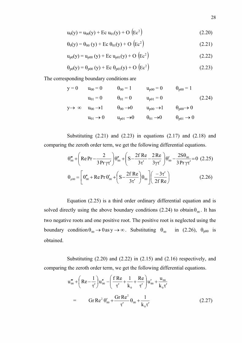
u0(y) = u00(y) + Ec u01(y) + O � �2Ec (2.20)
�0(y) = �00 (y) + Ec �01(y) + O � �2Ec (2.21)
up0(y) = up00 (y) + Ec up01(y) + O � �2Ec (2.22)
�p0(y) = �p00 (y) + Ec �p01(y) + O � �2Ec (2.23)
The corresponding boundary conditions are
y = 0 u00 = 0 �00 = 1 up00 = 0 �p00 = 1
u01 = 0 �01 = 0 up01 = 0 (2.24)
y) $ u00 )1 �00 )0 up00 )1 �p00) 0
u01 ) 0 up01 )0 �01 )0 �p01 ) 0
Substituting (2.21) and (2.23) in equations (2.17) and (2.18) and
comparing the zeroth order term, we get the following differential equations.
0Pr3S2
3Re2
3Ref2S
Pr32PrRe 00
000000 ���"
������
�
���
���"
���
��������
���
���"
��� ��� (2.25)
��
��� ���
��
���
��
�
���
������������
Ref23
3Ref2SPrRe 00000000p (2.26)
Equation (2.25) is a third order ordinary differential equation and is
solved directly using the above boundary conditions (2.24) to obtain . It has
two negative roots and one positive root. The positive root is neglected using the
boundary condition
00�
$))� yas000 . Substituting 00� in (2.26), �p00 is
obtained.
Substituting (2.20) and (2.22) in (2.15) and (2.16) respectively, and
comparing the zeroth order term, we get the following differential equations.
������
�
���
���
����
�����
���
�������
0
0000
00000 k
uuRek1Refu1Reu
= ��
����
���0
00
2
002
k1ReGrReGr (2.27)

29
��
��� ���
��
���
�����
�
���
��
��������
Refk1ReGru
k1RefuReuu
000
200
0000000p (2.28)
Equation (2.27) is a third order differential equation and is solved
directly using the boundary condition (2.24) to obtain u00. It has one negative
root and two positive roots. The positive roots are neglected using the boundary
condition. Substituting in (2.28), up00 is obtained. Thus the solutions are, 00u
ym2
ym100
21 eAeA �� ���
ym4
ym300p
21 eAeA �� ���
1eAeAeAu ym7
ym6
ym500
213 ���� ���
1eAeAeAu ym10
ym9
ym800p
213 ���� ���
Comparing the coefficient of Ec in equations (2.15) and (2.17), we get
��"�
������
���
���"
���
��������
���
���"
��� ���Pr3S2
3Re2
3Ref2S
Pr32PrRe 01
010101
= 2000000 u
32uuPr2 ���"
����� (2.29)
��
��� ���
��
���
�����
���
������������
Ref23uPr
3Ref2SPrRe 2
0001010101p (2.30)
01
2
012
0
0101
00101
ReGrReGrkuuRe
k1Refu1Reu �
�������
������
�
���
���
����
�����
���
�������
(2.31)
��
��� ���
��
���
����
�
���
��
��������
RefReGru
k1RefuReuu 01
201
0010101p (2.32)
Equation (2.29) is third order differential equations and is solved
directly using the boundary condition (2.24) to obtain 01� . It has two negative
roots and one positive root. The positive root is neglected using the boundary
condition . Equation (2.31) has one negative root and two $))� yas001

30
positive roots. The positive roots are neglected using the boundary condition
.Substituting in (2.30), up01 is obtained as follows. $)) yas0u 01
01 A��
A�
01p A��
A�
01 Au �
A�
01p Au �
A�
01u
ym2e�
m( 1e�
m2e�
m( 1e�
m1e�
m2 2e�
m37 e�
43A
ym214
ym21312
ym11
131 eAeAAe ��� ���
y)mm(18
y)mm(17
y)m16
ym215
313222 eAeAAe ������ ���
ym222
ym221
y20
ym19
131 eAeAAe ��� ���
y)mm(26
y)mm(25
y)m24
ym223
313222 eAeAAe ������ ���
ym230
ym29
y28
ym27
323 eAeAAe ��� ���
y)mm(35
y)mm(34
y)mm(33
y32
ym231
3132211 eAeAeAAe ������� ����
ym241
ym240
ym239
ym38
yym36
213213 eAeAeAeAAe ����� �����y)mm(
44y)mm(y)mm(
42313221 eAee ������ ��
When � * 0, substituting (2.14) in equations (2.3) to (2.12) and
equating the coefficients of �, we get
0z
wyv 11 �
��
��� (2.33)
0z
wy
v 1p1p ��
��
��
(2.34)
� �11p21
2
21
2
1Re�01
1 uufzu
yu
Re1Gr
yuv
yu
���
����
���
���
���
����
���
�
� �+ ,100
u1uzcos�kRe
1��� (2.35)
� 11 �0p1p
1p uy
uv
yu
��
����
���
pu1�
(2.36)
� �0
1011p2
12
21
2
yv
��11
kRe)vzcosv(vvf
zv
Re1
yp
yv ��
����
����
���
���
����
����
� (2.37)
� 11p1p vv1
yv
���
��� � (2.38)

31
� � � �0
1011p2
12
21
211
kRewzcoswwwf
zw
yw
Re1
zp
yw ��
����
����
���
���
���
���
����
�
(2.39)
� 11p1p ww1
yw
���
��
� � (2.40)
� �11p110
1012
12
21
2
3Ref2S
yu
yuEcPr2
yPrRe
yvPrRe
zy
�����
�����
��
�
���
����
����
����
(2.41)
� �11p0
1p1
Pr32
ypv
yp
�����"
����
����
� (2.42)
The corresponding boundary conditions are
y = 0 u1 = 0 v1 = zcos�� w1 = 0 �1 = 0
up1 = 0 vp1 = zcos�� wp1 = 0 �p1=1
(2.43)
y) $ u1)0 w1) 0 p1)0 �1) 0
up1)0 wp1)0 �p1) 0
Equations (2.37) – (2.40) are independent of the temperature field.
So, in view of the boundary conditions, applying separation of variables method,
it is assumed that
v1 (y,z) = -v11(y) cos�z vp1(y,z) = -vp11 (y) cos�z
zsin)y(v1)z,y(w 111 ���
� zsin)y(v1)z,y(w 11p1p ���
� (2.44)
p1 (y,z) = p11(y) cos�z
The equations (2.44) are so chosen such that the continuity equations
(2.33) and (2.34) are satisfied. Substituting (2.44) in equations (2.37) - (2.40)
and simplifying, we get

32
110
02
110
21111 v
k1kvRe
k1Refv1Rev ��
�
���
�����
�����
���
���
����
�������
���
�������
��
����
�����0
1111 k1pRepRe (2.45)
(2.46) 0pp 112
11 �����
��
��� ���
��
���
�����
�
���
��
����������
Refk1pRev
k1RefvRevv
01111
0
2111111p (2.47)
The corresponding boundary conditions are
y = 0 v11 = 1 011 ��v vp11 = 1 011 ��pv (2.48)
y) $ ) 011v� 11pv� )0 p11) 0
Equation (2.45) and (2.46) are ordinary differential equations and are
solved directly using the boundary condition (2.47). The solutions are given by y
111 eBp ���
4y
3yA
211 BeBeBv ��� ���
7y
6yA
511p BeBeBv ��� ���
In view of the boundary conditions, separation of variables method
can be applied for u and �. It is assumed that
u1(y,z) = u11(y) cos�z up1(y,z) = up11(y) cos�z
�1(y,z) = �11(y) cos�z �p1(y,z) = �p11(y) cos�z (2.49)
Substituting (2.49) in (2.35), (2.36), (2.41) and (2.42) and
simplifying, we get
110
02
110
21111 u
k1kuRe
k1Refu1Reu ��
�
���
�����
�����
���
���
����
�������
���
�������
= 11p0p0
011
2110110 vuRef
kuReGrvuRevuRe �
���
����������
)1u(k
1ReGrvuRe
00
11
2
110 ���
����
����
� (2.50)

33
��
��� ���
�����
�
�
�����
�
������
���
���
��
���������
�Ref
)1u(k1ReGrvuRe
uk1RefuReu
u
00
112
110
110
21111
11p (2.51)
112
1111 S3
Re23
Ref2Pr3
2PrRe �����
���
��
��"�
����������
�
���
���"
��� ���
� �11011011p0p11
2
uu3
Ec4v3
Re2v3
Ref2Pr3
S2 ����"
�����"
�����
����"
��� (2.52)
� � � �110110011011 uuuuEcPr2vvPrRe ������������� ���
��
��� ���
���
�
�
���
�
��������
���
���
��������� ��
��Ref23
SuuEcPr2vPrRe3
Ref2PrRe
11110011
112
111111p (2.53)
The corresponding boundary conditions are
y = 0 u11 = 0 �11 =0 up11 = 0 �p11 = 0
y ) $ u11 )0 �11 )0 up11 )0 �p11 ) 0 (2.54)
Now expanding u11 and �11 in powers of Ec as a series, we get,
u11 = u110 +Ec u111 + O( ) 2Ec
up11 = up110 +Ec up111 + O( ) 2Ec
�11 = �110 + Ec �111 + O( ) 2Ec
�p11= �p110 + Ec �p111 + O( ) (2.55) 2Ec
Substituting (2.55) in equations (2.50) – (2.53) and comparing zeroth
order term, we get,
1102
110110 S3
Re23
Ref2Pr3
2PrRe �����
���
��
��"�
����������
�
���
���"
��� ���
)vv(PrRev3
Re2v3
Ref2Pr3
)S(200110011001100p11p110
2
�����������"�
�����
����"
��� (2.56)
34
��
��� ���
���
�
������
��� �
�������������
Ref23vPrReSRefPrRe 0011110
2110110110p (2.57)
1100
02
1100
2110110 u
k1kuRe
k1Refu1Reu ��
�
���
�����
�����
���
���
����
�������
���
�������
00p11p0
00110
200110011 uvRef
kuReGruvReuvRe �
���
������������
� 1uk
1ReGruvRe
000
110
2
0011 ���
����
����
� � (2.58)
� ���
��� ���
���
���
�
���
��
������
���
���
��
���������
�Ref
1uk1ReGruvRe
uk1RefuReu
u
000
1102
0011
1100
2110110
110p (2.59)
The corresponding boundary conditions are
y = 0 u110 = 0 �110 =0 up110 = 0 �p110 = 0 (2.60)
y) $ u110)0 �110 )0 up110 ) 0 �p110 ) 0
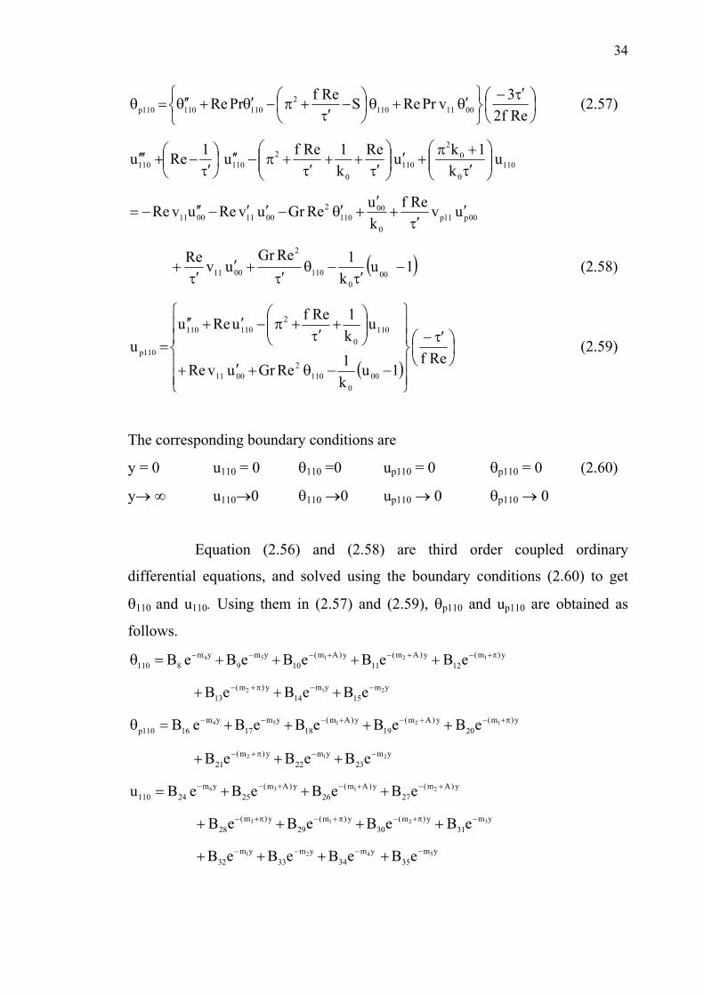
Equation (2.56) and (2.58) are third order coupled ordinary
differential equations, and solved using the boundary conditions (2.60) to get
�110 and u110. Using them in (2.57) and (2.59), �p110 and up110 are obtained as
follows. y)m(
12y)Am(
11y)Am(
10ym
9ym
811012154 eBeBeBeBeB ��������� ������
ym15
ym14
y)m(13
212 eBeBeB ����� ���
y)m(20
y)Am(19
y)Am(18
ym17
ym16110p
12154 eBeBeBeBeB ��������� ������
ym23
ym22
y)m(21
212 eBeBeB ����� ���
y)Am(27
y)Am(26
y)Am(25
ym24110
2136 eBeBeBeBu ������� ����
31y)m(
30y)m(
29y)m(
28213 BeBeBeB ��������� ����
ym35
ym34
ym33
ym32
5421 eBeBeBeB ���� ����
ym3e�
35
y)Am(39
y)Am(38
y)Am(37
ym36110p
2136 eBeBeBeBu ������� ����
ym43
y)m(42
y)m(41
y)m(40
3213 eBeBeBeB ���������� ����
ym47
ym46
ym45
ym44
5421 eBeBeBeB ���� ����
Comparing the coefficient of Ec in equations (2.50) – (2.53), we get
1112
111111 S3
Re23
Ref2Pr3
2PrRe �����
���
��
��"�
����������
�
���
���"
��� ���
11001011101p11p111
2
uu3
4v3
Re2v3
Ref2Pr3
)S(2 ����"
�����"
�����
����"
��� (2.61)
)uuuu(Pr2)vv(PrRe 110001100001110111 ����������������
��
��� ���
���
� ��������
�
��� �
�������������
Ref23uuPr2vPrReS
3Ref2PrRe 110000111111
2111111111p
(2.62)
1110
02
1110
2111111 u
k1kuRe
k1Refu1Reu ��
�
���
�����
�����
���
���
����
�������
���
�������
= 01p11p0
01111
201110111 uvRef
kuReGruvReuvRe �
���
�����������
����
����
���
0
01111
2
0111 kuReGr
uvRe (2.63)
��
��� ���
���
�
��������
���
��
����������
RefkuReGruvReu
k1RefuReuu
0
01111
20111111
0
2111111111p
(2.64)
The corresponding boundary conditions are
y = 0 u111 = 0 up111 =0 �111 = 0 �p111 = 0
y) $ u111) 0 up111 )0 �111 ) 0 �p111 ) 0 (2.65)
Equation (2.61) and (2.63) are third order coupled ordinary
differential equations, and solved using the boundary conditions (2.65) ) to get
36
�111 and u111. Using them in (2.62) and (2.64), �p111 and up11 are obtained. The
solutions are
y)mm(82
y)mm(81
y)mm(80
y)mm(79
y)mm(78
y)mm(77
y)mm(76
y)mm(75
y)mm(74
y)mm(73
y)mm(72
y)mm(71
ym270
ym269
ym268
ym67
ym66
y)mm(65
y)mm(64
y)mm(63
y)m2(62
y)m2(61
y)m2(60
y)m(59
y)m(58
y)Amm(57
y)Amm(56
y)Amm(55
y)Am2(54
y)Am2(53
y)Am2(52
y)Am(51
y)Am(50
ym49
ym48111
52
51534241
43626163
3132212
132131
322121
32131
322121
32154
eBeBeBeBeBeBeBeBeB
eBeBeBeBeBeBeBeBeB
eBeBeBeBeBeBeBeB
eBeBeBeBeBeBeBeBeB
��
��������
��������
�������
��������
��������������
������������
����������
��������
�
����
����
����
�����
����
����
����
������
y)mm(117
y)mm(116
y)mm(115
y)mm(114
y)mm(113
y)mm(112
y)mm(111
y)mm(110
y)mm(109
y)mm(108
y)mm(107
y)mm(106
ym2105
ym2104
ym2103
ym102
ym101
y)mm(100
y)mm(99
y)mm(98
y)m2(97
y)m2(96
y)m2(95
y)m(94
y)m(93
y)Amm(92
y)Amm(91
y)Amm(90
y)Am2(89
y)Am2(88
y)Am2(87
y)Am(86
y)Am(85
ym84
ym83111p
525153
4241436261
633132212
13213132
212132
13132212
132154
eBeBeBeBeBeBeBeB
eBeBeBeBeBeBeBeBeBeBeB
eBeBeBeBeBeBeBeBeBeB
eBeBeBeBeBeB
������
����������
���������
������������
����������������
��������������
����������
���
�����
�����
������
�����
�����
�������
ym156
ym155
y)mm(154
y)mm(153
y)mm(152
y)mm(151
y)mm(150
y)mm(149
y)mm(148
y)mm(147
y)mm(146
y)mm(145
y)mm(144
y)mm(143
ym2142
ym2141
ym2140
ym139
ym138
ym137
y)mm(136
y)mm(135
y)mm(134
y)m2(133
y)m2(132
y)m2(131
y)m(130
y)m(129
y)m(128
y)Amm(127
y)Amm(126
y)Amm(125
y)Am2(124
y)Am2(123
y)Am2(122
y)Am(121
y)Am(120
y)Am(119
ym118111
5452515342
4143626163
31322121
321331
322121
321331
322121
32136
eBeBeBeBeBeBeBeBeBeBeB
eBeBeBeBeBeBeBeBeBeB
eBeBeBeBeBeBeBeBeB
eBeBeBeBeBeBeBeBeBu
����������
����������
��������
��������
��������������
���������������
����������
���������
������
�����
�����
�����
����
�����
����
�����
37
ym195
ym194
y)mm(193
y)mm(192
y)mm(191
y)mm(190
y)mm(189
y)mm(188
y)mm(187
y)mm(186
y)mm(185
y)mm(184
y)mm(183
y)mm(182
ym2181
ym2180
ym2179
ym178
ym177
ym176
y)mm(175
y)mm(174
y)mm(173
y)m2(172
y)m2(171
y)m2(170
y)m(169
y)m(168
y)m(167
y)Amm(166
y)Amm(165
y)Amm(164
y)Am2(163
y)Am2(162
y)Am2(161
y)Am(160
y)Am(159
y)Am(158
ym157111p
5452515342
4143626163
31322121
321331
322121
321331
322121
32136
eBeBeBeBeBeBeBeBeBeBeB
eBeBeBeBeBeBeBeBeBeB
eBeBeBeBeBeBeBeBeB
eBeBeBeB
eBeBeBeBeBu
����������
����������
��������
��������
��������������
���������������
����������
���������
������
�����
�����
�����
����
�����
����
�����
where the constants are not given for the sake of brevity.
2.5.1 Skin – friction coefficient
The skin friction coefficient at the surface in the x* - direction is given
by
zcos)0()0(UV 10x
*
������#�
��
Where 0y
*
*
x*y
u
����
���
���
(��� is the shear stress.
2.5.2 Nusselt Number
The rate of heat transfer in terms of nusselt number Nu at the surface
is given by zcos)0(Nu)0(Nu)TT(C
qNu 10wP
����$�#&
��
Where 0y
*
*
*yTkq
����
���
���
��
2.6 RESULTS AND DISCUSSION
As the exact solutions are very lengthy, the velocity and temperature
of the fluid and the dust particles are shown through graphs, by incorporating the
exact solutions in the graph directly.
38
Some results for the fluid phase temperature profile and the particle
phase temperature profile
�
p� , the fluid velocity u and the particle velocity
based on the analytical solutions reported above are presented in figures 2.1
through 2.9. These results presented illustrate the influence of some of the
physical parameters on the solutions. The values of some of the physical
parameters employed to obtain the graphical result may or may not represent
actual conditions of applications.
pu
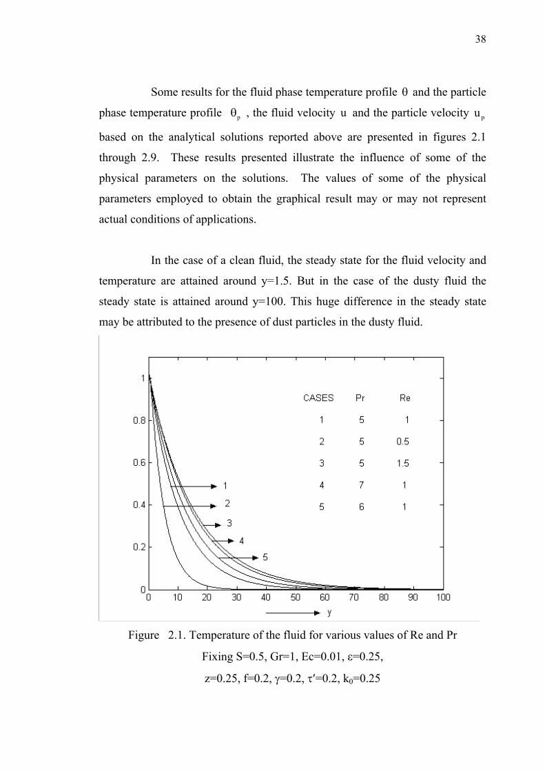
In the case of a clean fluid, the steady state for the fluid velocity and
temperature are attained around y=1.5. But in the case of the dusty fluid the
steady state is attained around y=100. This huge difference in the steady state
may be attributed to the presence of dust particles in the dusty fluid.
Figure 2.1. Temperature of the fluid for various values of Re and Pr
Fixing S=0.5, Gr=1, Ec=0.01, �=0.25,
z=0.25, f=0.2, "=0.2, ��=0.2, k0=0.25
39
2.6.1 Temperature profiles of fluid phase for various values of Re and Pr
A close look at figure.2.1 shows that the profiles of temperature of
the fluid increase with increase in both the Prandtl Number Pr and Reynolds
Number Re. They all start from 1 at the lower end of the plate and decrease
gradually to zero as y increases for all values of Re and Pr.
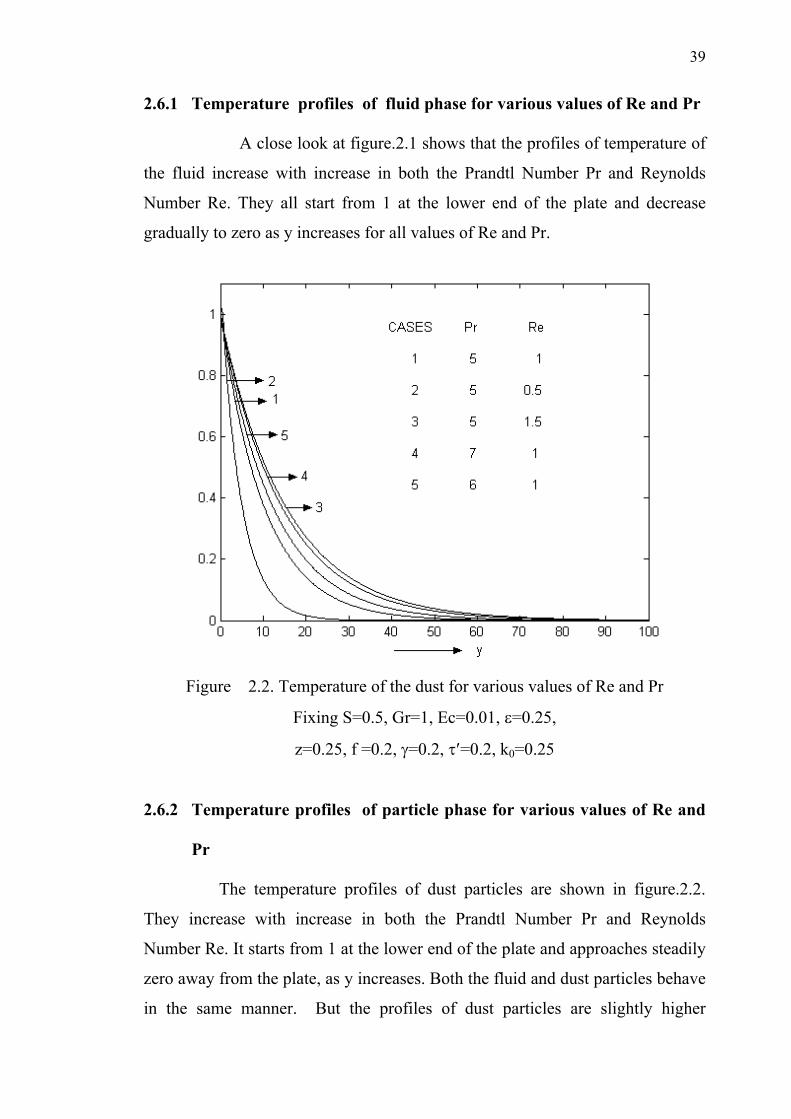
Figure 2.2. Temperature of the dust for various values of Re and Pr
Fixing S=0.5, Gr=1, Ec=0.01, �=0.25,
z=0.25, f =0.2, "=0.2, ��=0.2, k0=0.25
2.6.2 Temperature profiles of particle phase for various values of Re and
Pr
The temperature profiles of dust particles are shown in figure.2.2.
They increase with increase in both the Prandtl Number Pr and Reynolds
Number Re. It starts from 1 at the lower end of the plate and approaches steadily
zero away from the plate, as y increases. Both the fluid and dust particles behave
in the same manner. But the profiles of dust particles are slightly higher

40
compared with that of the fluid. In the case of clean fluid, the temperature
profiles decrease with increase in Reynolds Number and Prandtl Number
whereas in the case of a dusty fluid the profiles decrease with increase in these
two parameters. This phenomenon may be due to the influence of dust particles.
Figure 2.3. Velocity of the fluid for various values of Re and Pr
Fixing S=0.5, Gr=1, Ec=0.01, �=0.25,
z=0.25, f =0.2, "=0.2, ��=0.2, k0=0.25
2.6.3 Velocity profiles of the fluid phase for various values of Re and Pr
From figure 2.3, it can be concluded that increase in Reynolds
Number and Prandtl Number increases the velocity profile of the fluid for some
fixed values of other parameters. The velocity profiles maintain an increasing
trend near the lower end of the plate and attain their maximum very near the
lower end and thereafter they decrease steadily and reach the value 1 as y
approaches 100. In the case of clean fluid, the velocity profiles increase steadily
from zero and reach the value 1 as y increases.
41
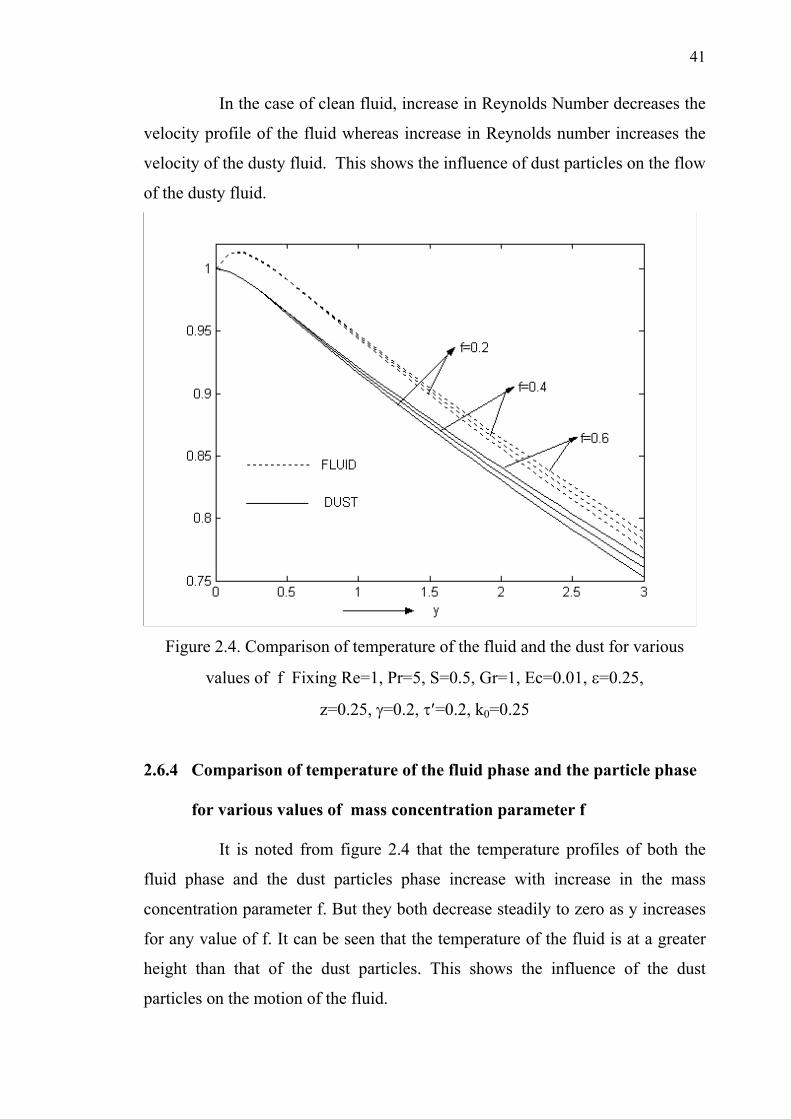
In the case of clean fluid, increase in Reynolds Number decreases the
velocity profile of the fluid whereas increase in Reynolds number increases the
velocity of the dusty fluid. This shows the influence of dust particles on the flow
of the dusty fluid.
Figure 2.4. Comparison of temperature of the fluid and the dust for various
values of f Fixing Re=1, Pr=5, S=0.5, Gr=1, Ec=0.01, �=0.25,
z=0.25, "=0.2, ��=0.2, k0=0.25
2.6.4 Comparison of temperature of the fluid phase and the particle phase
for various values of mass concentration parameter f
It is noted from figure 2.4 that the temperature profiles of both the
fluid phase and the dust particles phase increase with increase in the mass
concentration parameter f. But they both decrease steadily to zero as y increases
for any value of f. It can be seen that the temperature of the fluid is at a greater
height than that of the dust particles. This shows the influence of the dust
particles on the motion of the fluid.

42
Figure 2.5. Velocity of the fluid for various values of f
Fixing Re=1, Pr=5, S=0.5, Gr=1, Ec=0.01, �=0.25,
z=0.25, " =0.2, ��=0.2, k0=0.25
2.6.5 Velocity of the fluid phase for various values of mass concentration
parameter f
It is observed from figure 2.5 that the velocity profiles of the fluid
phase increase steadily for increase in the mass concentration parameter f. As y
increases the velocity profiles of the fluid phase goes on increasing upto 1.4
nearly and then maintain a decreasing trend and reach the value 1. As the
profiles of the velocity of the fluid phase are very significant upto y=3, the
graphs are drawn upto y=3.
43
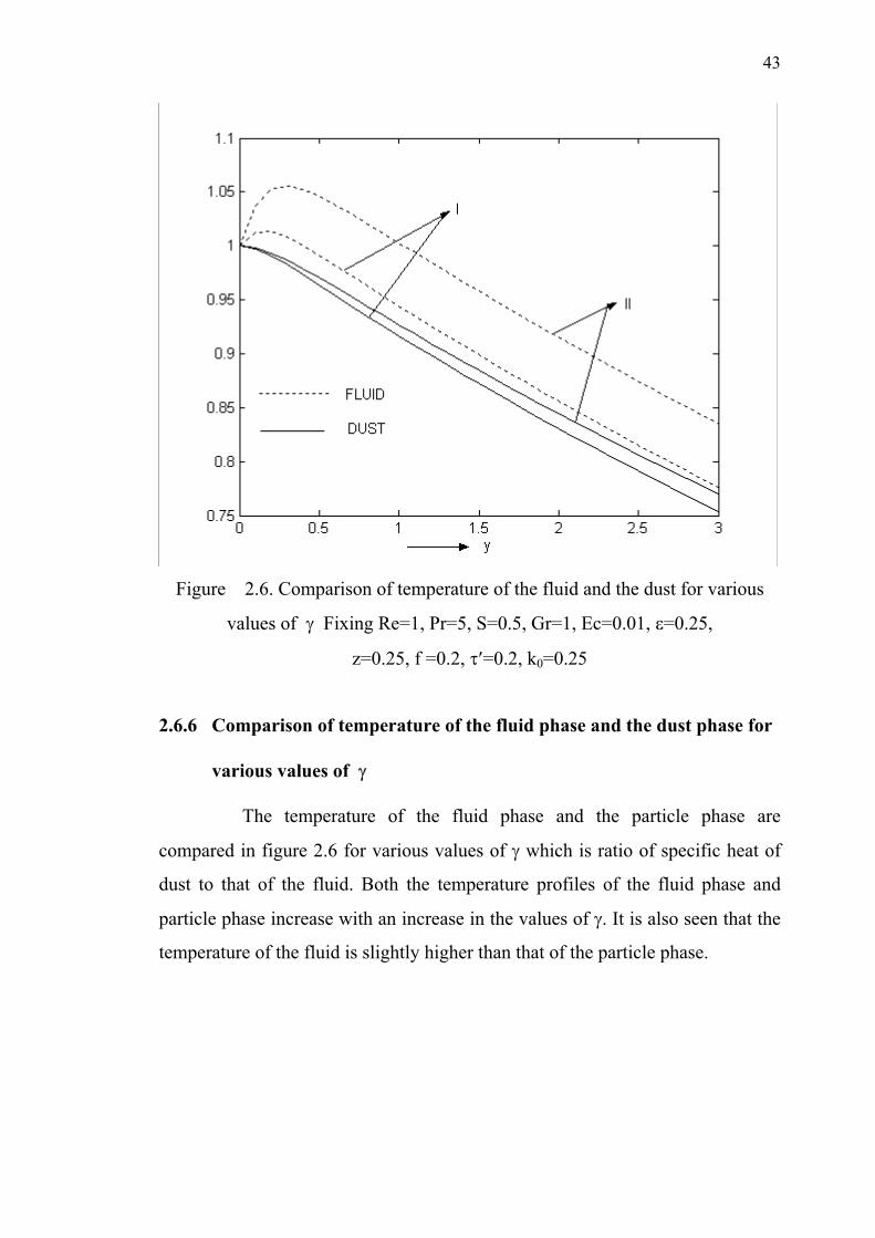
Figure 2.6. Comparison of temperature of the fluid and the dust for various
values of " Fixing Re=1, Pr=5, S=0.5, Gr=1, Ec=0.01, �=0.25,
z=0.25, f =0.2, ��=0.2, k0=0.25
2.6.6 Comparison of temperature of the fluid phase and the dust phase for
various values of "
The temperature of the fluid phase and the particle phase are
compared in figure 2.6 for various values of " which is ratio of specific heat of
dust to that of the fluid. Both the temperature profiles of the fluid phase and
particle phase increase with an increase in the values of ". It is also seen that the
temperature of the fluid is slightly higher than that of the particle phase.

44
Figure 2.7. Velocity of the fluid for various values of "
Fixing Re=1, Pr=5, S=0.5, Gr=1, Ec=0.01, �=0.25,
z=0.25, f =0.2, ��=0.2, k0=0.25
2.6.7 Velocity of the fluid phase for various values of "
The velocity profiles of the fluid phase are shown in figure 2.7 for
various values of" . It is noted from figure 2.7. that the velocity profiles of the
fluid phase decrease with an increase in the value of " which is ratio of specific
heat of the dust to that of the fluid. As the profiles show a significant difference
very near the lower end of the plate, the graphs is drawn upto y=3. As y
increases the velocity of the fluid phase increases till y=3 and then they will
decrease to reach the value 1. The cases I and II in figures 2.6 and 2.7 are as
given in the following table 2.1.

45
Table 2.1 Cases I and II represented in figure 2.7 and 2.8
CASES " I
II
0.2
0.4
Figure 2.8. Comparison of temperature of the fluid and the dust for various
values of �� Fixing Re=1, Pr=5, S=0.5, Gr=1, Ec=0.01, �=0.25,
" =0.2, z=0.25, f =0.2, k0=0.25
2.6.8 Comparison of temperature of the fluid phase and the dust phase for
various values of� � , the time relaxation parameter.
The temperature profiles of the fluid phase and the particle phase are
compared in figure 2.8 for various values of� � , the time relaxation parameter. It
is seen that the temperature profiles of both the fluid phase and the particle phase
increase as � � increases. Also it can be noted that the fluid temperature is
slightly higher than the particle temperature for any value of� � . The temperature
profiles of both phases maintain a decreasing trend as y increases.

46
Figure 2.9.Velocity of the fluid for various values of ��
Fixing Re=1, Pr=5, S=0.5, Gr=1, Ec=0.01, �=0.25,
" =0.2, z=0.25, f =0.2, k0=0.25
2.6.9 Velocity of the fluid phase for various values of � � , the time
relaxation parameter
The velocity profiles of the fluid phase are shown in figure in 2.9. It
is observed that the velocity profiles of the fluid phase increase with an increase
in the values of time relaxation parameter. As y increases, the velocity profiles
increase up to 1.4 nearly and thereafter will decrease steadily and reach the value
1. As the curves show significant difference near the lower end, the curves have
been drawn up to y=3.
47
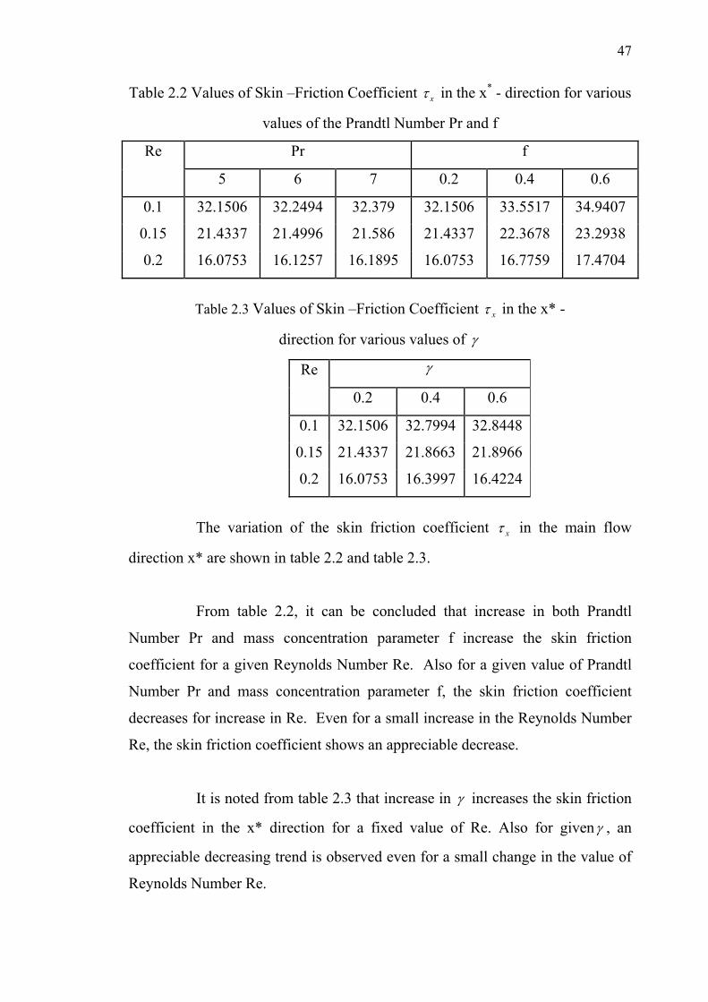
Table 2.2 Values of Skin –Friction Coefficient x� in the x* - direction for various
values of the Prandtl Number Pr and f
Pr f Re
5 6 7 0.2 0.4 0.6
0.1 32.1506 32.2494 32.379 32.1506 33.5517 34.9407
0.15 21.4337 21.4996 21.586 21.4337 22.3678 23.2938
0.2 16.0753 16.1257 16.1895 16.0753 16.7759 17.4704
Table 2.3 Values of Skin –Friction Coefficient x� in the x* -
direction for various values of "
" Re
0.2 0.4 0.6
0.1 32.1506 32.7994 32.8448
0.15 21.4337 21.8663 21.8966
0.2 16.0753 16.3997 16.4224
The variation of the skin friction coefficient x� in the main flow
direction x* are shown in table 2.2 and table 2.3.
From table 2.2, it can be concluded that increase in both Prandtl
Number Pr and mass concentration parameter f increase the skin friction
coefficient for a given Reynolds Number Re. Also for a given value of Prandtl
Number Pr and mass concentration parameter f, the skin friction coefficient
decreases for increase in Re. Even for a small increase in the Reynolds Number
Re, the skin friction coefficient shows an appreciable decrease.
It is noted from table 2.3 that increase in " increases the skin friction
coefficient in the x* direction for a fixed value of Re. Also for given" , an
appreciable decreasing trend is observed even for a small change in the value of
Reynolds Number Re.
48
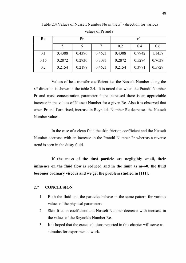
Table 2.4 Values of Nusselt Number Nu in the x* - direction for various
values of Pr and� �
Pr � � Re
5 6 7 0.2 0.4 0.6
0.1 0.4308 0.4396 0.4621 0.4308 0.7942 1.1458
0.15 0.2872 0.2930 0.3081 0.2872 0.5294 0.7639
0.2 0.2154 0.2198 0.4621 0.2154 0.3971 0.5729
Values of heat transfer coefficient i.e. the Nusselt Number along the
x* direction is shown in the table 2.4. It is noted that when the Prandtl Number
Pr and mass concentration parameter f are increased there is an appreciable
increase in the values of Nusselt Number for a given Re. Also it is observed that
when Pr and f are fixed, increase in Reynolds Number Re decreases the Nusselt
Number values.
In the case of a clean fluid the skin friction coefficient and the Nusselt
Number decrease with an increase in the Prandtl Number Pr whereas a reverse
trend is seen in the dusty fluid.
If the mass of the dust particle are negligibly small, their
influence on the fluid flow is reduced and in the limit as m)0, the fluid
becomes ordinary viscous and we get the problem studied in [111].
2.7 CONCLUSION
1. Both the fluid and the particles behave in the same pattern for various
values of the physical parameters
2. Skin friction coefficient and Nusselt Number decrease with increase in
the values of the Reynolds Number Re.
3. It is hoped that the exact solutions reported in this chapter will serve as
stimulus for experimental work.