chapter 9 decisions, actions, and...
TRANSCRIPT

199
Chapter 9 DECISIONS, ACTIONS, AND GAMES
While we have now developed separate logics for knowledge update, belief revision, or
preference change, concrete instances of rational agency bring in all three entangled. The
most concrete setting where this happens is in games, and therefore, this chapter is mainly
devoted to the question how we can use our earlier logics to describe the latter interactive
scenarios. We will be discussing both the logical statics, viewing games as unchanging
structures representing all possible runs of some process, and the dynamics which arises
when we make things happen on such a ‘stage’. As we shall see, this involves a mixture of
two different faces of logic, or even two different tribal communities, hard-core logics of
computation and philosophical logics of belief and preference. But it is precisely this
surprising mixture which makes current theories of agency and interaction so lively.
We start with a few examples showing what we are interested in eventually. Then we move
to a series of standard logics describing static game structure, from moves to preferences
and epistemic uncertainty. More toward the end of the chapter, we introduce the earlier
dynamic logics, and see what they have to add in scenarios involving information update
and belief revision where given games can change as new information arrives. This chapter
is meant to make a connection. It is by no means a full treatment of logical perspectives on
games, for which we refer to the companion volume van Benthem, to appear.
9.1 Decisions, practical reasoning, and games
Action and preference Even the simplest scenarios of practical reasoning about agents
involve a number of notions at the same time. Recall this example from Chapter 8:
Example One single decision.
An agent has two alternative courses of action, but prefers one outcome to the other:
a b
x ! y
A proto-typical form of reasoning here would be the ‘Practical Syllogism’:

200
(i) the agent can do both a and b,
(ii) the agent prefers the result of a over the result of b,
and therefore,
(iii) the agent will do [or maybe: should do?] b. !
This predictive inference, or maybe requirement, is in fact the basic notion of rationality
for agents throughout a vast literature in philosophy, economics, and many other fields. It
can be used to predict behaviour beforehand, or rationalize observed behaviour afterwards.
Adding beliefs Decision scenarios crucially involve all our notions so far. Preference
occurs intertwined with action, and a reasonable way of taking the conclusion is, not as
knowledge ruling out courses of action, but as supporting a belief that the agent will take
action b: the latter event is now more plausible than the world where she takes action a.
Thus, modeling even very simple decision scenarios involves logics of different kinds.
Beliefs come in even more strongly closer to actual decision theory. There, decisions are
modeled with uncertainty about possible states of nature, and we are told to choose the
action with the highest expected value, a probabilistically weighted sum of utility values for
the various outcomes. The probability distribution over states of nature represents beliefs
we have about the world, or the behaviour of an opponent. Here is an yet simpler scenario:
Example Deciding with an external influence.
Nature has two moves c, d, and the agent must now consider combined moves:
a, c b, c a, d b, d
x y z u
Now, the agent might already have good reasons to think that Nature’s move c is more
plausible than move d. This will turn the outcomes into an epistemic-doxastic model in the
style of Chapter 6: the epistemic range has 4 worlds, but the most plausible ones are just 2:
x, y, while the agent’s preference might now just refer to the latter area. !

201
Thus, we get the entanglement discussed in Chapter 8, while we also see the earlier point in
Chapter6 that it is our beliefs which guide our actions. Here is a typical scenario for this.
Multi-agent decision: ‘solving’ games by Backward Induction In a multi-agent setting,
behaviour is locked in place by mutual expectations. This requires an interactive decision
dynamics, and standard game solution procedures like Backward Induction do exactly this
sort of thing. Again, recall an earlier example from Chapter 8:
Example Reasoning about interaction.
In the following game tree, players’ preferences are encoded in the utility values, as pairs
‘(value of A, value for E)’. Backward Induction tells player E to turn left when she can,
just like in our single decision case, which gives A a belief that this would happen, and
therefore, based on this belief about his counter-player, A should turn left at the start: A
1, 0 E
0, 100 99, 99
Why should players act this way? The reasoning is again a mixture of all notions so far.
A turns left since she believes that E will turn left, and then her preference is for grabbing
the value 1. Thus, practical reasoning intertwines action, preference, and belief. !
Here is the rule which drives all this, at least when preferences are encoded numerically:
Definition Backward Induction algorithm.
Starting from the leaves, one assigns values for each player to each node, using the rule
Suppose E is to move at a node, and all values for daughters are known. The E-value is the
maximum of all the E-values on the daughters, the A-value is the minimum of the A-values
at all E-best daughters. The dual calculation for A’s turns is completely analogous. !
This rule is so obvious that it never raises objections when taught, and it is easy to apply,
telling us what players’ best course of action would be (Osborne & Rubinstein 1994). And
yet, it is packed with various assumptions. We will perform a ‘logical deconstruction’ of
theunderlying reasoning in this chapter, but for now, just note the following features:

202
(a) the rule assumes that the situation is viewed in the same way by both players:
since the calculations are totally similar,
(b) the rule assumes worst-case behaviour on the part of one’s opponents,
since we take a minimum of values in case it is not our turn,
(c) the rule changes its interpretation of the values: at leaves they encode plain
utilities, while higher up in the game tree, they represent expected utilities.
Thus, in terms of our earlier chapters, we would say that, despite the numerical trappings,
Backward Induction is really an inductive mechanism for generating a plausibility order
among histories, and hence, it relates our models in Chapter 6 to those of Chapter 8:
betterness and plausibility order become intertwined in a systematic manner. It is this sort
of situation which we should study eventually in the logic of games.
But for now, we step back, and look at what ‘logic of games’ would involve ab initio,
starting without any preferences at all. So, let us first consider pure action structure, since
even that has a good deal of logic to it, which can be brought out as such. 146 We will add
further preferential and epistemic structure toward more realistic games in due course.
9.2 Games and process equivalence
In this chapter, we view extensive games as multi-agent processes which can be studied
just like any process in logic and computer science, given the right logical language.
Technically, such structures are models for a poly-modal logic in a straightforward sense:
Definition Extensive games.
An extensive game form is a tree M = (NODES, MOVES, turn, end, V) which is a modal
model with binary transition relations taken from the set MOVES pointing from parent to
daughter nodes. Also, intermediate nodes have unary proposition letters turni indicating the
unique player whose turn it is, while end marks end nodes without further moves. The
valuation V for proposition letters may also interpret other relevant predicates at nodes,
such as utility values for players or more external properties of game states. !
146 Our treatment will be a sketch: for details see the companion volume van Benthem, to appear.

203
But do we really just want to jump on board of this analogy, comfortable as it is to a modal
logician? Just to emphasize how close, indeed, this setting is to our earlier style of analysis,
here is a fundamental issue of invariance we raised before in Chapter 2. At which level do
we want to operate in the logical study of games, or in more Clintonesque terms: When are two games are the same?
Example The same game, or not?
As a simple example that is easy to remember, consider the following two games: A E
L R L R
p E A A
L R L R L R
q r p q p r
Are these the same? As with general processes in computer science (cf. Chapter 2), the
answer crucially depends on our level of interest in the details of what is going on: (a) If we focus on turns and moves, then the two games are not equivalent.
For they differ in ‘protocol’ (who gets to play first) and in choice structure. For instance,
the first game, but not the second has a stage where it is up to E to determine whether the
outcome is q or r. This is indeed a natural level for looking at game, involving local actions
and choices, as encoded in modal bisimulations – and the appropriate language will be a
standard modal one. But one might also want to call these games equivalent in another
sense: looking at achievable outcomes only, and players powers for controlling these:
(b) If we focus on outcome powers only, then the two games are equivalent.
The reason is that, regardless of protocol and local choices, players can force the same sets
of eventual outcomes across these games, using strategies that are available to them:
A can force the outcome to fall in the sets {p}, {q, r},
E can force the outcome to fall in the sets {p, q}, {p, r}.
In the left-hand tree, A has 2 strategies, and so does E, yielding the listed sets. In the right-
hand tree, E has 2 strategies, while A has 4: LL, LR, RL and RR. Of these, LL yields the

204
outcome set {p}, and RR yields {q, r}. But LR, RL guarantee only supersets {p, r}, {q, p} of
{p}: i.e., weaker powers. Thus the same 'control' results in both games. !
In this book, we will concentrate on the extensive modal level, but we do note that the
coarser power level is natural, too. It is closer to the ‘strategic forms’ for games employed
in game theory, and also, it fits very well with ‘logic games’ (cf. our companion volume
van Benthem, to appear). We take our leave of the latter connection with one illustration:
Remark: game equivalence as logical equivalence In an obvious sense, the two games in
the preceding example represent the two sides of the following valid logical law p ! (q"r) # (p!q) " (p!r) Distribution Just read conjunction and disjunction as choices for different players. In a global input–
output view, Distribution switches scheduling order without affecting players’ powers. !
9.3 Basic modal action logic of extensive games
Henceforth, we will restrict attention to extensive games in the modal style.
Basic modal logic On extensive game trees, a standard modal language works as follows: Definition Modal game language and semantics.
Modal formulas are interpreted at nodes s in game trees M. Labeled modalities <a>$
express that some move a is available leading to a next node in the game tree satisfying $.
Proposition letters true at nodes may be special-purpose constants for game structure, such
as indications for turns and end-points, but also arbitrary local properties. !
In particular, modal operator combinations now describe potential interaction:
Example Modal operators and strategic powers.
Consider a simple 2-step game like the following, between two players A, E: A
a b
E E
c d c d
1 2 3 4
p p

205
Player E clearly has a strategy making sure that a state is reached where p holds. And this
feature of the game is directly expressed by the modal formula [a]<d>p ! [b]<c>p. !
More generally, letting move stand for the union of all relations available to players, in the
preceding game, the modal operator combination [move-A]<move-E>$ says that, at the current node of evaluation, player E has a strategy for responding to A's
initial move which ensures that the property expressed by $ results after two steps of play. 147 This fundamental relation between strategic structure and logical operator combinations
is crucial to so-called ‘logic games’, a topic for which we refer to van Benthem 2007.
Excluded middle and determinacy Extending this observation to extensive games up to
some finite depth k, and using alternations !!!!... of modal operators up to length k, we
can express the existence of winning strategies in fixed finite games. Indeed, given this
connection, with finite depth, standard logical laws have immediate game-theoretic import.
In particular, consider the valid law of excluded middle in the following modal form
!!!!...$ " ¬!!!!...$
or after some logical equivalences, pushing the negation inside:
!!!!...$ " !!!!...¬$,
where the dots indicate the depth of the tree. Here is its game-theoretic import:
Fact Modal excluded middle expresses the determinacy of finite games.
Here, determinacy is the fundamental property of many games that one of the two players
has a winning strategy. This need not be true in infinite games (players cannot both have
one, but maybe neither has), and descriptive set theory has deep theory around this notion.
Zermelo’s theorem This brings us to perhaps the oldest game-theoretic result proved in
mathematics, even predating Backward Induction, proved by Ernst Zermelo in 1913:
147 One can also express the existence of ‘winning strategies’, ‘losing strategies’, and so forth.

206
Theorem Every finite zero-sum 2-player game is determined.
Proof Here is a simple algorithm determining the player having the winning strategy at any
given node of a game tree of this finite sort. It works bottom-up through the game tree.
First, colour those end nodes black that are wins for player A, and colour the other end
nodes white, being the wins for E. Then extend this colouring stepwise as follows:
If all children of node s have been coloured already, do one of the following:
(a) if player A is to move, and at least one child is black:
colour s black; if all children are white, colour s white
(b) if player E is to move, and at least one child is white:
colour s white; if all children are black, colour s black
This procedure eventually colours all nodes black where player A has a winning strategy,
while making those where E has a winning strategy white. And the reason for its
correctness is that a player has a winning strategy at one of her turns iff she can make a
move to at least one daughter node where she has a winning strategy. !
Zermelo's Theorem is widely applicable. Recall the Teaching Game from our Introduction:
Example Teaching, the grim realities.
A Student located at position S in the next diagram wants to reach the escape E below,
while the Teacher wants to prevent him from getting there. Each line segment is a path that
can be traveled. In each round of the game, the Teacher cuts one connection, anywhere,
while the Student can, and must travel one link still open to him at his current position:
S X
Y E General education games like this arise on any graph with single or multiple lines. !
We now have a principled explanation why either Student or Teacher has a winning
strategy, since this game is obviously two-player zero sum and of finite depth – though
there need be an effective computational method for solving the game. Zermelo’s Theorem

207
implies that in Chess, one player has a winning strategy, or the other a non-losing one – but
almost a century later, we do not know which is which: the game tree is just too large. 148
9.4 Fixed-point languages for equilibrium notions
A good test for logical languages is checking their expressive power for rendering proofs of
significant results. Here our basic modal language seems a bit poor, since it cannot express
the generic character of the Zermelo solution. He following is what the colouring
algorithm really says. Starting from atomic predicates wini at end nodes indicating which
player has won, we inductively defined predicates WINi (‘player i has a winning strategy at
the current node’) through the following recursion: WINi # (end & wini) " (turni & <E> WINi) " (turnj & [A] WINi)
Here E is the union of all available moves for player i, and A that of all moves for the
counter-player j. This schema is an inductive definition for the predicate WINi , which we
can also write as a smallest fixed-point expression in an extended modal language:
Fact The Zermelo solution is definable as follows in the modal µ–calculus: WINi = µp• (end & wini) " (turni & <E> p) " (turnj & [A]p) 149
Here the formula on the right-hand side belongs to the modal µ–calculus, an extension of
the basic modal language with operators for smallest (and greatest) fixed-points defining
inductive notions. This system was originally invented to increase the power of modal logic
as a process theory. We refer to the literature for details, cf. Bradfield & Stirling 2007, van
Benthem 2008. For here, we just observe that fixed-points fit well with strategic equilibria,
and the µ–calculus has many further uses in games (cf. Chapter 14 for another example).
As we said already in the global perspective of Section 9.2, games are all about powers of
control which players have over ‘reachable propositions’ via their strategies:
148 But the clock is ticking for Chess. Recently, for the game of Checkers, 15 years of real-time
computer verification yielded the Zermelo answer: the starting player has a non-losing strategy. 149 Note that the defining schema only has syntactically positive occurrences of the predicate p.

208
Definition Forcing modalities.
Forcing modalities are interpreted as follows in extensive game models as defined earlier:
M, s |= {i}$ iff player i has a strategy for the sub-game starting at s which guarantees that
only nodes will be visited where $ holds, whatever the other player does. !
Forcing talk is widespread in games, and it is an obvious target for logical formalization: 150 Fact The modal µ–calculus can define forcing modalities. Proof The formula {i}$ = µp• (end & $) " (turni & <E> p) " (turnj & [A]p) defines the
existence of a strategy for i ensuring that proposition $ holds, whatever the other plays. !
But many other notions are definable. For instance, the recursion COOP $ # µp• (end & $) " (turni & <E> p) " (turnj & <A>p)
defines the existence of a cooperative outcome $, just by shifting some modalities. 151
Digression: from smallest to greatest fixed-points The above modal fixed-point definitions
reflect the equilibrium character of basic game-theoretic notions (Osborne & Rubinstein
1994), reached through some process of iteration. In this general setting, which includes
infinite games, we would switch from smallest to greatest fixed-points, as in the formula {i}$ = %q• ($ & (turni & <move-i>q) " (turnj & [move-j]q)). This is also more in line with our intuitive view of strategies. The point is not that they are
built up from below, but that they can be used as needed, and then remain at our service as
pristine as ever the next time – the way we think of doctors. This is the modern perspective
of co-algebra (Venema 2007). More generally, greatest fixed-points seem the best logical
analogue to the standard equilibrium theorems from analysis that are used in game theory.
150 Note that {i}$ talks about intermediate nodes, not just end nodes of a game. The existence of a
winning strategy for player i can then be formulated by restricting to endpoints: {i} (end ! wini). 151 This fixed point can still be defined in propositional dynamic logic, using the formula < ((turni)?
; E ) & (turnj)? ; A )) *] (end & $), – but we will only use the latter system later in the game setting.

209
But why logic? This may be a good place to ask the question what is the point of giving
logical definitions of game-theoretic notions? The way I see this chapter, logic has the
same virtues for games as it has elsewhere. Through formalization of a given practice, we
see more clearly what makes its key notions tick, and we also get a feel for new alternative
notions, as the logical language has myriads of possible definitions. Moreover, the theory
of expressive power, completeness, and complexity of our logics can be used for model
checking, proof search, and other activities not normally associated with game theory. But there is also another viewpoint: not central to this book on information dynamics, but
equally important in general. As we saw in Chapter 2, basic notions of logic themselves
have a game character, such as argumentation, model checking, or model comparison.
Thus, logic does not just describe games, it also embodies games. When we pursue the
interface in this dual manner, the true grip of the logic & games connection becomes clear,
and this will be the main thrust of the companion volume van Benthem, to appear.
9.5 Dynamic logics of strategies
Given that strategies, rather than single moves, are obvious protagonists in our story, it
makes sense to move them into our logics. This requires another extension of modal logic,
viz. propositional dynamic logic (PDL, Bradfield & Stirling 2007) used for analyzing
conversation in Chapter 3, and for common knowledge in Chapter 5. PDL was created to
describe the structure and effects of imperative computer programs constructed using the
sequential operations of (a) sequential composition ;, (b) guarded choice IF ... THEN...
ELSE..., and (c) guarded iterations WHILE... DO... We recall some earlier definitions: Definition Propositional dynamic logic.
The language of PDL defines formulas and programs in a mutual recursion, with formulas
denoting sets of worlds (‘local conditions’ on ‘states’ of the process), while programs
denote binary transition relations between worlds, recording pairs of input and output states
for their successful terminating computations. Programs are created from atomic actions (‘moves’) a, b, … and tests ?' for arbitrary formulas ',
using the three operations of ; (interpreted as sequential composition),
& (non-deterministic choice) and * (non-deterministic finite iteration).

210
Formulas are as in our basic modal language, but with modalities [(]' saying that ' is true
after every successful execution of the program ( starting at the current world. !
The logic PDL is decidable, and it has an transparent complete set of axioms for describing
validity which we will give later. Right here, our point is that this formalism can say a lot
more about our preceding examples. For instance, the move relation in our discussion of
our first extensive game in this chapter was really a union of atomic transition relations,
and the pattern that we discussed for the winning strategy was as follows: [a&b] <c&d>p.
Strategies as transition relations But we can deal with strategies much more explicitly.
Game-theoretic strategies may be viewed as partial transition functions defined on players'
turns, given via a bunch of conditional instructions of the form "if she plays this, then I
play that". More generally, strategies may be viewed as binary transition relations, allowing
for non-determinism, i.e., more than one ‘optimal move’. While this is not the standard
approach in game theory, such a relational view comes much closer to plans that agents
have in interactive settings. A plan can be extremely useful, even when it merely constrains
my future moves, without necessarily fixing my course of action. Thus, on top of the ‘hard-
wired’ move relations in a game, we now get defined further relations, corresponding to
players’ strategies, and these definitions can often be given explicitly in a PDL-format.
In particular, in finite games, we can define an explicit version of the earlier forcing
modality, indicating the strategy involved – without recourse to the modal µ–calculus: Fact For any game program expression ), PDL can define an explicit forcing
modality {), i}$ stating that ) is a strategy for player i forcing the game,
against any play of the others, to pass only through states satisfying $. The precise definition is an easy exercise (cf. van Benthem 2002). Also, given strategies for
both players, we should get to a unique history of a game, and here is how:
Fact Outcomes of running joint strategies ), * can be defined in PDL.

211
Proof The formula [((?turnE ; )) & (?turnA ; * )) *] (end + p) does the job. 152 !
But also, on a model-by-model basis, the expressive power of PDL for defining specific
strategies is high. Consider any finite game M with a strategy ) for player i. As a relation,
) is a finite set of ordered pairs (s, t). Thus, it can be defined by enumeration as a program
union, if we define these ordered pairs. To do so, assume we have an ‘expressive’ model
M, where states s are definable in our modal language by formulas defs. 153 Then we define
transitions (s, t) by formulas defs; a; deft, with a being the relevant move:
Fact In expressive finite extensive games, all strategies are PDL-definable. Of course, this is a trivial result, but it does suggest that PDL is on the right track. Dynamic
logic can also define strategies running over only part of a game, and their combination.
The following modal operator describes the effect of such a partial strategy ) for player E
running until the first game states where it is no longer defined: {), E}$ [(?turnE ; ) ) & (?turnA ; move-A) *] $
A basic operation on partial strategies would be intersection, leaving only moves allowed
by both. Van Benthem 2002 discusses Relational Algebra as a form of strategy calculus.
Van Benthem 2007 is a full-fledged survey and defense of modal logics with explicit
strategies. Indeed, propositional dynamic logic does a reasonable job in defining explicit
strategies in simple extensive games. 154 In the next sections, we will extend it to deal with
more realistic game structures, such as preferences and imperfect information.
152 Dropping the antecedent ‘end +’ here will describe effects of strategies at intermediate nodes.
153 This expressive power can be achieved in several ways: e.g., using temporal past modalities
over converse moves which can describe the total history leading up to s. 154 Stronger modal logics of strategies? The modal µ-calculus is a natural extension of PDL, but it
lacks explicit programs or strategies, as its formulas merely define properties of states. Is there a
version of the µ--calculus which extends PDL in defining mre transition relations? Say, a simple
strategy ‘keep playing a’ guarantees infinite a-branches for greatest fixed-point formulas like %p•
<a>p. Van Benthem & Ikegami 2008 look at richer fragments than PDL with explicit programs as
solutions to fixed-point equations of special forms, guaranteeing uniform convergence by stage ,.

212
9.6 Preference logic and defining backward induction Real games, as we have seen several times already, go beyond mere game forms by adding
preferences for players over outcome states, or numerical utilities beyond ‘win’ and ‘lose’.
In this area, defining the earlier-discussed Backward Induction procedure for solving
extensive games, rather than computing binary Zermelo winning positions, has become a
benchmark for game logics – and many solutions exist:
Fact The Backward Induction path is definable in modal preference logic.
Solutions have been published by many logicians and game-theorists in recent years, cf. de
Bruin 2004, van der Hoek & Pauly 2007. We do not state an explicit PDL-style solution
here, but we give one version involving the modal preference language of Chapter 8: <prefi>$ : player i prefers some node where $ holds to the current one. The following result from van Benthem, van Otterloo & Roy 2006 defines the backward
induction path as a unique relation ): not by means of any specific modal formula in game
models M, but rather via the following frame correspondence on finite structures:
Fact The BI strategy is definable as the unique relation ) satisfying the following
axiom for all propositions P – viewed as sets of nodes –, for all players i:
(turni & <)*>(end & P)) + [move-i]<)*>(end & <prefi>P). Proof The axiom expresses a form of rationality: at the current node, no alternative move
for a player guarantees outcomes that are all strictly better than the outcomes ensuing from
playing the current backward induction move. The proof of this frame correspondence is a
straightforward induction on levels of the finite game tree. !
9.7 Epistemic logic of games with imperfect information
The next level of static structure gives up aother presupposition made in this chapter so far,
that of perfect information for players concerning their situation. Consider extensive games
with imperfect information, whose players need not know where they are in the game tree.
This happens in card games, electronic communication, and real life game scenarios with
bounds on memory or observation. Such games have ‘information sets’: equivalence
classes of epistemic relations ~i between nodes which players i cannot distinguish, as in the

213
S5-type models of Chapters 2–5. Van Benthem 2001 points out how these games model a
combined epistemic modal language including knowledge operators Ki$ interpreted in the
usual manner as "$ is true at all nodes ~i–related to the current one".
Example Partial observation in games.
In this imperfect information game, a dotted line indicates player E's uncertainty about her
position when her turn comes. Thus, she does not know the move played by player A: 155 A
a b
E E E
c d c d
1 2 3 4
p p !
Structures like this are game models of the earlier kind with added epistemic uncertainty
relations ~I for each player. Thus, they interpret a combined dynamic-epistemic language.
For instance, after A plays move c in the root, in both middle states, E knows that playing a
or b will give her p – as the disjunction <a>p " <b>p is true at both middle states: KE (<a>p " <b>p)
On the other hand, there is no specific move of which E knows at this stage that it will
guarantee a p–outcome – and this shows in the truth of the formula ¬KE<a>p & ¬KE<b>p
Thus, E knows de dicto that she has a strategy which guarantees p, but she does not know,
de re, of any specific strategy that it guarantees p. Such finer distinctions are typical for a
language with both actions and knowledge for agents. 156
We can analyze imperfect information games studying properties of players by modal
frame correspondences. An example is an earlier analysis of Perfect Recall for a player i:
155 Maybe A put his move in an envelope, or E was otherwise prevented from observing. 156 You may know that the ideal partner for you is around on the streets, but tragically, you might
never convert this K- combination into -K knowledge that some particular person is right for you.

214
Fact The axiom Ki[a]$ + [a]Ki$ holds for player i w.r.t. any proposition $
iff M satisfies Confluence: .xyz: (( xRay & y~iz) + -u: (( x~iu & uRaz).
Similar frame analyses work for memory bounds, and observational powers for agents (van
Benthem 2001). For instance, in the opposite direction of Perfect Recall, agents satisfy the
principle of ‘No Miracles’ when their epistemic uncertainty relations can only disappear
when they observe two subsequent events which they can distinguish. 157 Incidentally, the
game which we just gave does satisfy Perfect Recall, but it violates No Miracles, since E
suddenly knows exactly where she is after she has played her move. We will discuss these
properties in much greater generality in the epistemic-temporal logics of Chapter 11.
Uniform strategies Another striking aspect of the above game with imperfect information
is its non-determinacy. E’s playing ‘the opposite direction from that chosen by player A’
was a strategy guaranteeing outcome p in the original game – but it is unusable now. For,
E cannot tell if the condition holds! Game theorists only accept uniform strategies here,
prescribing the same move at indistinguishable nodes. But then no player has a winning
strategy, when we interpret p as ‘E wins’ (and hence ¬p as a win for player A). A did not
have one to begin with, E loses hers. The game does have probabilistic solutions in random
strategies: 158 essentially, it is like Matching Pennies, but we do not pursue these here.
Now once again for explicit strategies! As before, we can add PDL-style programs here to
define players’ strategies under the new circumstances. But there is a twist. Especially
relevant then are the 'knowledge programs' of Fagin et al. 1995, whose only test conditions
for actions are knowledge statements for agents. In such programs, the actions prescribed
for an agent can only be guarded by conditions which the agent knows to be true or false. It
is easy to see that knowledge programs can only define uniform strategies, i.e., transition
relations where a player always chooses the same move at any two game nodes which she
cannot distinguish epistemically. A converse also holds, modulo some assumptions on
expressiveness of the game language defining nodes in the game tree (van Benthem 2001):
157 Our analysis restates that of Halpern & Vardi on epistemic-temporal logic (Fagin et al. 1995).
158 Both players should play both moves with probability ", for an optimal outcome 0.

215
Fact On expressive finite games of imperfect information, the uniform strategies
are precisely those definable by knowledge programs in epistemic PDL.
9.8 From statics to dynamics: DEL-representable games
Now we make a switch. We have linked logic to games in various ways, but our approach
was static in the sense of Chapter 1, using modal-preferential-epistemic logics to describe
properties of given games, which themselves do not change. While this is in line with the
literature in the area, it also makes sense to look at dynamic scenarios in the sense of this
book, where games themselves can change because of certain triggering events. But as an
intermediate step toward that goal, we now first analyze how a static game model might
have come about as the result of some dynamic process – the way we see a dormant
volcano but can also imagine the tectonic forces that shaped it originally. The present and
the next section provide two illustrations of this perspective, linking games of imperfect
information first to DEL (Chapter 4), and then to epistemic-temporal logics (Chapter 11).
Imperfect information games and dynamic-epistemic logic The reader should long have
seen the connection between imperfect information games and the product update system
DEL of our Chapter 4, as it creates successive models starting from some initial one. For a
start, as with adding preferences, there are two levels for making the earlier action logic
PDL epistemic. One can connect worlds, as with the above language with standard
epistemic modalities Ki. But one can also place epistemic structure on the moves
themselves, as in dynamic epistemic logic. This at once raises the issue which imperfect
information games ‘make sense’ in terms of real scenarios from dynamic-epistemic logic,
as opposed to being just arbitrary placements of uncertainty links over game forms:
What sort of imperfect information games correspond to the update evolution
of some initial model using product update as in dynamic-epistemic logic?
Theorem An extensive game tree is isomorphic to a repeated product update model
Tree(M, E) over some epistemic event model E iff it satisfies, for all players:
(a) Perfect Recall,
(b) (uniform) No Miracles,

216
(c) Bisimulation Invariance for the domains of the move relations. 159
Here Perfect Recall is essentially the earlier commutation property between moves and
uncertainty. We do not prove the Theorem here, as an extensive version will be presented
in Chapter 11 below (van Benthem & Liu 2004, van Benthem, Gerbrandy & Pacuit 2007
have definitions and proofs). Instead, here is an illustration. We can create an imperfect
information game for DEL-style players by first specifying preconditions and observation
structure on the moves, and then producing the game tree through iterated product update:
Example Updates during play: propagating ignorance along a game tree.
Game tree Event model
A a E b c precondition: turnA
a b c d A e f precondition: turnE
E E E
d e e f f
Here are the successive updates that create the right uncertainty links:
stage 1
stage 2 E
stage 3
A E !
9.9 Future uncertainty, procedural information, and branching temporal logic
A second logical perspective on games with imperfect information starts from the
following observation. The phrase ‘imperfect information’ covers two intuitively different
senses. One is observation uncertainty: players may not have been able to observe all
events so far, and so they do not know where they are in the game tree. This is the ‘past-
oriented’ view of DEL. But there is also ‘future-oriented’ expectation uncertainty, which
159 I.e., two epistemically bisimilar nodes in the game tree make the same moves executable.

217
occurs even in games of ‘perfect’ information players may know precisely where they are,
but they do not know where the game is heading as they do not know what others, or they
themselves, are going to do. The positive side of the situation is this. In general, players
will have a certain amount of procedural information about what is going to happen, and
van Benthem 2008 has argued that this is a fundamental and new notion of information
concerning the current process agents are in, which may be considered sui generis. But whether viewed negatively or positively, the latter future-oriented kind of knowledge
and ignorance need not be reducible to the earlier uncertainty between local nodes. Instead,
it naturally suggests current uncertainty between whole future histories, or between
players’ strategies (i.e., whole ways in which the game might evolve). The next points are
from van Benthem 2004 on information update and belief revision in game trees. Branching epistemic temporal models The following structure is common to many fields
in computer science and philosophy (cf. Chapter 11 below for more details). In tree-like
models for branching time, ‘legal histories’ h represent possible evolutions of a given
game. At each stage of the game, players are in a node s on some actual history whose past
they know, either completely or partially, but whose future is yet to be fully revealed: h'
s
h
This can be described in an action language with knowledge, belief, and added temporal
operators. We first describe games of perfect information (about the past, that is): (a) M, h, s |= Fa$ iff s/<a> lies on h and M, h, s/<a> |= $
(b) M, h, s |= Pa$ iff s = s' /<a>, and M, h, s' |= $
(c) M, h, s |= !i $ iff M, h', s |= $ for some h' equal for i to h up to stage s. Now, as moves are played publicly, players make public observations of them:

218
Fact The following valid principle is the temporal equivalent of the key DEL
reduction axiom for public announcement: Fa!$ # (FaT & !Fa$). 160
We will see this principle return as a recursion law for PAL with protocols in Chapter 11.
Trading future for current uncertainty in games Again, there is a possible ‘dynamic
reconstruction’ for these models, this time, providing an alternative description closer to
the local dynamics of PAL and DEL after all. Intuitively, each move by a player is a public
announcement that changes the current game. Here is a folklore observation converting
‘global’ uncertainty about the future into ‘local’ uncertainty about the present:
Fact Trees with future uncertainty are isomorphic to trees with current uncertainties. Proof The construction is this (cf. van Benthem 2004 for a slightly more formal version):
Given any game tree G, assign epistemic models Ms to each node s whose domain is the set
of complete histories passing through s (which all share the same past up to s), letting the
agent be uncertain about all of them. ‘Worlds’ in these models may be seen as pairs (h, s)
with h any history passing through s. This will cut down the current set of histories in just
the right manner. The above epistemic-temporal language matches this construction. !
9.10 Intermezzo: three levels of logical game analysis
At this point, it may be useful to distinguish three natural levels at which games have given
rise to models for logics. All three come with their own intuitions, both static and dynamic. Level One is the most straightforward perspective: extensive game trees themselves are
models for modal languages, with nodes as worlds, and accessibility relations over these
for actions, preferences, and uncertainty. Level Two rather looks at extensive games as
branching tree models, involving both nodes and complete histories, supporting richer
epistemic-temporal (-preferential) languages. The difference with Level One may seem
slight in finite extensive games, where histories may be marked by their end-points, so that
a point on a given history may also be viewed as just a pair of nodes. But the intuitive step
160 As in our earlier modal-epistemic analysis, commutation of a temporal and an epistemic operator
implies a form of Perfect Recall: agents' present uncertainties are always inherited from past ones.

219
from the first to the second perspective is clear, and also, Level Two cannot be reduced in
this manner when game trees are infinite. But even this is not enough for some purposes! Consider ‘higher’ hypotheses about the future, involving procedural information about
other players’ strategies. I may know that I am playing against either a ‘simple automaton’,
or a ‘sophisticated learner’. Modeling this may go beyond epistemic-temporal models: Example Strategic uncertainty.
In the following simple game, let A know that E will play the same move throughout: A
E E
Then all four histories are still possible. But A only considers two future trees possible, viz. A A
E E E E
In longer games, this difference in modeling can be highly important, because observing
only one move by E will tell A exactly what E’s strategy will be in the whole game. !
To model these richer settings, one needs full-fledged Level Three epistemic game models.
Definition Epistemic game models.
Epistemic game models for an extensive game G are epistemic models M = (W, ~i, V)
whose worlds are abstract indices including local (factual) information about all nodes in
G, plus whole strategy profiles for players, i.e., total specifications of everyone's behaviour
throughout the game. Players’ global information about game structure and procedure is
encoded by uncertainty relations ~i between the worlds of the game model. !
The above uncertainty between two strategies of my opponent would be naturally encoded
in constraints on the set of strategy profiles represented in such a model. And observing

220
some moves of yours in the game telling me which strategy you are actually following then
corresponds to dynamic update of the initial model, in the sense of our earlier chapters.
While we will not use Level-Three models much in this chapter, they are the natural limit
for games and other scenarios of interactive agency. Throughout this chapter, we follow
the policy of discussing issues at the simplest modeling level where they make sense.
9.11 Game change: public announcements, promises and solving games
Now let us look at actual transformations of given games, and explicit triggers for them.
Promises and intentions Following van Benthem 2007, one can break the impasse of a bad
Backward Induction solution by changing the game through making suitable promises.
Example Promises and game change.
In the following game, discussed several times before, the ‘bad Nash equilibrium’ (1, 0)
can be avoided by E’s promise that she will not go left, which may be modeled as a public
announcement that some histories will not occur (we may make this binding in a number of
ways, e.g., by attaching a huge fine to infractions) – and the new equilibrium (99, 99)
results, making both players better off by restricting the freedom of one of them!
A A
1, 0 E 1. 0 E
0, 100 99, 99 99, 99 !
But one can also add new moves to a game. 161 Van Otterloo 2005 has a dynamic logic of
strategic ‘enforceability’ plus preference, where game models can change by announcing
players’ intentions. Related scenarios let public announcements provide information about
players’ preferences. Our methods from Chapters 3 and following apply here at once:
161 Yes, in this way, one could code up all such game changes beforehand in one grand initial 'Super
Game' – but that would lose all the flavour of understanding what happens in a stepwise manner.

221
Theorem Modal logic of games plus public announcement is completely
axiomatized by the modal game logic chosen, the recursion axioms of PAL
for atoms and Booleans, plus the following law for the move modality:
<!P><a>' # (P ! <a>(P ! <!P>').
Strategies once more We can also talk about explicit strategies in all of this. Using PDL
for strategies in games as before, this leads to the obvious logic PDL+PAL adding public
announcements [!P]. It is easy to show that PDL is closed under relativization to definable
sub-models, both in its propositional and its program parts, using a recursive operation (|P
for programs ( which surrounds every atomic move with tests ?P.
Theorem PDL+ PAL is axiomatized by merging their separate laws while adding
the following reduction axiom: [!P]{)} $ # (P + {)|P}[!P]$). 162
But of course, we also want to know about versions with epistemic preference languages –
and hence there are many further questions following up on these initial observations.
Solving games by announcements of rationality Another type of application of public
announcement in games iterates assertions expressing that players are rational, as a sort of
‘public reminders’. Van Benthem 2003 has the following result for extensive games:
Theorem The Backward Induction solution for extensive games is obtained through
repeated announcement of the assertion "no player chooses a move all of whose
further histories end worse than all histories after some other available move".
Proof This can be proved by a simple induction on finite game trees. The principle behind
the argument will be clear by seeing how the announcement procedure works for the
following simple ‘Centipede game’, with three turns as indicated, four branches indicated
by name, and the pay-offs given for A, E in that order:
162 This axiom says what old plan I should have had to make some plan work in the new game. But
usually, I already have a plan ) for playing G to get effect $. Now G changes to G’: my game got
more, or fewer, moves. How should I revise that current plan ) to get some intended effect 0 in
the new game G'? This may be related to open model-theoretic problems like finding a Los-Tarski
theorem syntactically characterizing those PDL formulas which are preserved under sub-models.

222
A E A u 5, 5
x y z
1, 0 0, 5 6, 4
Stage 0 of the announcement procedure rules out branch u,
Stage 1 then rules out z, while Stage 2 finally rules out y. !
As in the analysis of iterated assertions in Chapter 3, this iterated announcement procedure
for extensive games (or for the temporal models of the preceding section) ends in largest
sub-models in which players have common belief of rationality, or other assertions. 163 Of course, our logical language provides many further assertions that can be announced,
far beyond the ruthless egotism of Backward Induction. Van Benthem 2003, 2004 discuss
history-oriented alternatives, where players steer future actions by reminding themselves of
legitimate rights of other players, because of ‘past favours received’. 164 165
The same ideas work in strategic games, with epistemic models M of strategy profiles with
preferences and uncertainties for players who know their own strategy, but not that of the
others. In Chapter 14, we formulate assertions of Weak Rationality (“no player chooses a
move which she knows to be worse than some other available one”) and Strong Rationality
(“each player chooses a move she thinks may be the best possible one”). When announced,
these assertions eliminate worlds, and iterating these announcements, perhaps infinitely,
one eventually gets to a smallest sub-model where WR or SR are common knowledge:
163 What about an epistemic-doxastic temporal preference language where the final sub-models can
be explicitly defined? Does it need fixed-point operators, like for strategic games in Chapter 14? 164 Type spaces for games, too, allow for much greater freedom in assumptions about players. 165 The different options are somewhat reminiscent of a distinction in social philosophy, between
Rawls’ forward-oriented adjustment view of fairness which recommends minimizing differences in
the current income distribution, versus Nozicks’ historical entitlement view, which say that a
current income distribution is fair if there was a history of fair transactions leading to it.

223
Theorem The result of iterated announcement of WR is the usual solution concept
of Iterated Removal of Strictly Dominated Strategies; and it is definable inside
M by means of a formula of a modal µ–calculus with inflationary fixed-points.
The same for iterated announcement of SR and game-theoretic Rationalizability. 166
9.12 Belief, update and revision in extensive games
So far, we have considered players’ knowledge in games, which came in various kinds,
past observation-based and future-oriented procedural. Next, we consider the concomitant
notion of belief, which can also have observational and procedural aspects. To do so, we
return to the models in Sections 9.7 through 9.9. Level-One models will add doxastic
structure using plausibility relations inside epistemic equivalence classes on the extensive
game tree, just as we did in Chapter 6 for belief revision. Intuitively, as we did with pure
knowledge, a game tree annotated with players’ beliefs in this way may be viewed as a
record of stepwise events of knowledge update and belief revision that take place as the
game is played, and we will return to this representational issue in Chapter 11.
For the moment, we elaborate another perspective, viz. the Level-Two view of branching
trees, a vivid way of modeling beliefs about the future which can be related to our earlier
belief update principles in several ways. Recall our earlier epistemic-temporal models for
branching time. We already saw how knowledge can be modeled, eliminating future
histories by public announcement of the current move, resulting in a recursion axiom
Fa!$ # (FaT & !Fa$)
This perspective is found in van Benthem 2004, where it is also extended to belief.
Beliefs over time We now add binary relations !I, s of state-dependent relative plausibility
between histories to branching temporal models. As in Chapter 6, we then get a doxastic
modality (existential here, for convenience), with both absolute and conditional versions:
166 As we note in Chapter 14, if the iterated assertion A has ‘existential-positive’ syntactic form
(for instance, SR does), the relevant definition can be formulated in the standard µ–calculus.

224
Definition Absolute and conditional belief.
We set M, h, s |= <B, i>$ iff M, h', s |= $ for some history h' coinciding with h up to
stage s and most plausible for i according to the given relation !I, s. As an extension, M, h, s
|= <B, i>0$ iff M, h', s |= $ for some history h' most plausible for i according to the
given !I, s among all histories coinciding with h up to stage s and satisfying M, h', s |= 0. !
For convenience, we mostly consider an absolute state-independent version of plausibility.
Now, belief revision happens as follows. Suppose we are at node s in the game, and move
a is played which is publicly observed. At the earlier-mentioned purely epistemic level,
this event just eliminates some histories from the current set. But there is now also belief
revision, as we move to a new plausibility relation !I, s^a describing the updated beliefs.
Hard belief update First, assume that plausibility relations are not node-dependent, making
them global. In that case, we have precisely belief revision under hard information, as
already analyzed in Chapter 6. The new plausibility relation is the old one, restricted to a
smaller set of histories. Here is the characteristic recursion law which governs this. To
understand it, recall that the temporal operator Fa' says that a is the next event on the
current branch, and that ' is true on the current branch immediately after a has taken place:
Fact The following temporal principles are valid for hard revision along a tree: Fa<B, i>$ # (FaT & <B, i>(FaT, Fa$))
Fa<B, i>0$ # (FaT & <B, i>(Fa0, Fa$))
Again, this is analogous to the dynamic doxastic recursion axioms for hard information in
Chapter 6. Behind the Fact lies a general assumption that the plausibility order has only
been restricted, not changed as a move is played. More abstractly, in the state-dependent
version, this may be viewed as a principle of Coherence which says that the most plausible
histories for i at h', s' are the intersection of Bt with all continuations of s'. 167
Soft update So far, our Level-Two belief dynamics is only driven by hard information, as
moves are observed. What would be a game analogue for events of soft information and
167 Similar principles have been stated in Bonanno 2007 which formalizes AGM theory.

225
matching plausibility changes among worlds, which were the more exciting theme in
Chapter 6? This richer setting seems to call for two additional features:
(a) models with the above state-dependent plausibility relations, so that a move
to a next state can change the plausibility pattern on the remaining histories,
(b) events beyond mere observable moves serving as soft triggers – say,
additional signals or ‘hunches’ that players receive in the course of a game.
This time, recursion axioms will not be ‘absolute’ like the preceding ones, but they will
reflect policies for plausibility change. We will not pursue this topic here – but in Chapter
11, we do consider the related issue of belief revision under soft information when the
plausibility relation runs, not between whole histories, but nodes of the branching tree.
More local dynamics What would be most in line with the spirit of this book, however, are
concrete stepwise procedures creating beliefs and preferences as we proceed along an
extensive game tree. An interesting recent approach of this sort is given in Baltag, Smets &
Zvesper 2008, which use assertions of ‘dynamic rationality’ to define those epistemic-
doxastic models where plausibility relations for players encode the Backward Induction
solution – with ‘intended moves’ indicated by strategies at most plausible worlds. This
analysis is not yet quite what we are looking for here, since it works over global Level-
Three models encoding all game behaviour beforehand in the worlds, while there are no
genuine events of soft update corresponding to real belief revision as the game proceeds.
9.13 Further entanglements: dynamics of rationalization
Finally, as we have noticed several times so far, knowledge and belief are entangled
notions, and the entanglement even extends to preference (cf. Chapter 8). Many issues in
applying or interpreting games reflect this situation, starting with the solution procedure of
Backward Induction itself. We will discuss a few more, just to loosen up the reader’s mind
as to what should eventually be described by the logics of this chapter. Here are a few
dynamic scenarios from van Benthem 2007 extending well-known facts about games.
Observed actions and rationalization Rationality in the sense of decision theory and game
theory often has its greatest successes, not in predicting behaviour in advance, but in

226
rationalizing it afterwards. We do this all the time. If your preferences between outcomes
of some game are not known, I can always ascribe a preference which makes your action
rational, by assuming you prefer the outcome of the chosen action over the others. This
style of rationalization carries over to more complex interactive settings. But now one must
also think about Me, i.e., the player you are interacting with. The following seems folklore.
Let a finite two-player extensive game G specify my preferences, but not yours. Moreover,
let our strategies )me, ) you for playing G be fixed in advance, yielding an expanded game
model M. All this is supposed to be common knowledge. 168 When can we rationalize your
given behaviour )you to make )me, )you the Backward Induction (‘BI’) solution of the game?
To achieve this, we have total freedom to set your preferences between outcomes of the
game, independently from my given ones. Even so, not all models M of this sort support
rationalization toward Backward Induction. My given actions encoded in )me must have a
certain quality to begin with, related to my preferences. Note that, at any node of the game
tree, playing on according to our given strategies fixes a unique outcome of the game.
What is clearly necessary for any successful BI-style analysis is the following version of
the rationality assertion that we used for analyzing Backward Induction in Section 9.9:
Definition Best-responsiveness.
A game is best-responsive for Me given two strategies )me, )you if my )me always chooses a
move leading to an outcome which is at least as good for me as any other outcome that
might arise by choosing any other move, and then continuing with the given )me, )you. !
Theorem In any finite game model as described that is best-responsive for Me, there
exists a preference relation for You among outcomes that makes the unique path
playing our given strategies against each other the Backward Induction solution.
Proof One starts with final choices for players at the bottom of the game tree, assigning
values reflecting preferences for you as described. (My choice was ‘rational’ automatically,
given best-responsiveness.) Now proceed inductively. As my turns higher up in the tree are
best-responsive for Me, I am consistent with BI, as the strategies in the sub-games after my
168 We do just a few dynamic scenarios here: the reader will see many options for variations.

227
moves are already in accordance with BI. Next, let it be your turn, with the same inductive
assumption. In particular, these sub-games already have BI-values for both you and me.
Now suppose your prescribed move a in )you leads to a sub-game Ga with a lower BI-value
for You than some other available move. In that case, a simple trick makes a best for you.
Take some fixed number N large enough so that adding N to your utility in all outcomes of
Ga makes them better than all outcomes reachable by your other moves than a. Now note:
Raising all your values of outcomes in a game tree by a fixed amount N
does not change the BI-solution, though it raises your total value by N. Doing this to a's subtree, your given move at this turn has become best. !
Example Rationalizing given strategies.
The procedure runs bottom-up. Bold face arrows mark your given moves, dotted arrows
mine. Bold-face numbers at leaves indicate values for outcomes that we postulate for You.
Think of your value 2, 3 to the left in (b) as BI-values assigned by the procedure already –
while mine are not indicated (but we can assume my choice are best-responsive): You You You
3 Me 3 Me 3 Me
You 2 You 2 You 4
0 1 2 3
(a) (b) (c) [N=2]
Of course, these numbers can be assigned in many ways to get BI right. !
Given actions and postulated beliefs Here is another dynamic scenario. We just used BI to
rationalize given strategies in a game G, and implicitly, players’ beliefs, postulating
preferences for one of the players. Now, we start from given preferences for both players,
and modify the beliefs of the players to rationalize the given behaviour.
Example Adjusting beliefs with given preferences.
Suppose you choose Right in our game with the ‘bad outcome’ (1, 0):

228
A
1, 0 E
0, 100 99, 99
One can interpret this rationally if we assume you believe I will go Right in the next move.
This rationalization is not in terms of your preferences, but of your beliefs about me. 169 !
Again, this readjustment procedure only works under conditions like the rationality used in
Secion 9.9. Consider a finite game model M with your strategy )you and your preference
relation given (mine does not matter). Suppose You can choose move Left or Right, but all
outcomes of Left are better for You than all those arising after Right. Then no beliefs of
yours about my subsequent moves can make a choice for Right come out ‘best’:
Definition ‘Minimally rational’ game models.
A game model is minimally rational for You if your strategy )you never prescribes a move
for which each outcome reachable via further play according to )you and any sequence of
moves of Me is worse than all outcomes reachable via some other move for You. 170 !
The following result is a counterpart to our PAL-style analysis of BI in Section 9.9:
Theorem In any game model that is minimally rational for You, there is a strategy *
for Me against which, if you believe that I will play *, your given )you is optimal.
Proof This time, the procedure for finding a rationalizing * is top-down. Suppose you make
a move a right now according to your strategy. Since )you is minimally rational for you,
each alternative move b of yours must have at least one reachable outcome y (via )you plus
some suitable sequence of moves for me) which is majorized by some reachable outcome x
via a. In particular, your maximum value reachable by playing a always majorizes some
value in each sub-game for another move. Now we describe a strategy for Me which makes
your given move a optimal. Choose later moves for Me in the subgame for a which lead to
169 Note that this belief-based style of rationalizing need not produce the ‘standard’ BI solution. 170 In case you are the last player to move, this coincides with standard rationality again..
229
the outcome x, and choose moves for Me leading to outcomes y ! x in the subgames for my
other moves b. This makes sure that a is a best response against any strategy of mine that
includes those moves. This does not yet fully determine the strategy that you believe I am
going to play, but one can proceed downward along the given game tree. !
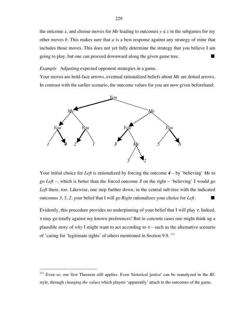
Example Adjusting expected opponent strategies in a game.
Your moves are bold-face arrows, eventual rationalized beliefs about Me are dotted arrows.
In contrast with the earlier scenario, the outcome values for you are now given beforehand:
You
Me Me
You You You You
1 4 2 1 3 Me 5 6
5 2
Your initial choice for Left is rationalized by forcing the outcome 4 – by ‘believing’ Me to
go Left –, which is better than the forced outcome 3 on the right – ‘believing’ I would go
Left there, too. Likewise, one step further down, in the central sub-tree with the indicated
outcomes 3, 5, 2, your belief that I will go Right rationalizes your choice for Left. !
Evidently, this procedure provides no underpinning of your belief that I will play *. Indeed,
* may go totally against my known preferences! But in concrete cases one might think up a
plausible story of why I might want to act according to * – such as the alternative scenario
of ‘caring for ‘legitimate rights’ of others mentioned in Section 9.9. 171
171 Even so, our first Theorem still applies. Even 'historical justice' can be reanalyzed in the BI-
style, through changing the values which players ‘apparently’ attach to the outcomes of the game.

230
9.14 Conclusion
We have shown how games involve a combination of all the logics that we have discussed
so far, including knowledge, belief, and preference. We gave pilot studies rather than grand
logical theory, though some of the above themes will be taken up again and elaborated in
Chapters 11 and 14. But even at this stage, we hope to have shown that logical dynamics
and games is an exciting area for research with both formal structure and intuitive appeal.
9.15 Appendix: further topics and open problems
Designing concrete knowledge games The games studied in this chapter are all abstract.
But many epistemic and doxastic scenarios in earlier chapters also suggest concrete games,
say, of ‘being the first to know’ certain important facts under constraints in observation and
communication. It would be of interest to have such ‘gamifications’ of our dynamic logics.
Game equivalence with preference added Taking preference structure seriously would
give many topics in our earlier sections a new twist. For instance, van Benthem 2002
considers the issue ‘when two games are the same’ when preference structure is present,
looking at intuitions like ‘supporting the same strategic equilibria’. These deviate
considerably from earlier notions like modal bisimulation, or ‘power equivalence’.
Preferences between actions? Games also suggest a new issue, which would have made
sense in Chapter 8 already, about combining propositional dynamic logic and preference
logic. Since PDL has formulas as properties of states and programs as inter-state relations,
we can put preference structure at two levels. One kind runs between states, interpreting
standard modal operators as in Chapter 8, which focused on comparison between worlds.
The other locus is preferences between state transitions (‘moves’, ‘events’) as in van der
Meijden 1996, van Benthem 1999. Compare the distinction in ethics between ‘deontology’
and ‘consequentialism’. Do we compare the worlds resulting from actions when judging
our duties, or do we qualify those actions themselves as ‘better’ or ‘obligatory’? Games
suggest a preference logic directly on moves, and our guess is that this can be developed in
a manner analogous to our dynamic-epistemic logic DEL in Chapter 5 with product update
for events, perhaps using rules more like the priority update of Chapter 6.

231
Knowledge that and know-how Taking strategies seriously also raises new issues, such as
the famous distinction between ‘knowing that’ and ‘knowing how’. Strategies are ways of
achieving goals, and hence they represent procedural know-how. What does it mean to
‘know a strategy’ in epistemic dynamic logics, and can we develop significant logics of
strategies in games with imperfect information? Chapter 13 studies some of these issues,
including epistemically transparent strategies ) with the property that, when part of ) has
been played, players still know that playing the rest will achieve the intended result.
Local dynamics inside given games We already mentioned the lack of a local marriage of
DEL style events and moves in extensive games, tighter than what we have provided here.
Soft update in games Our dynamic scenarios involved mostly public observation of moves.
What natural extension of games would support the soft information events of Chapter 6?
Agent diversity and memory We characterized the DEL-like games of imperfect
information in terms of players with Perfect Recall. But there are many others, such as the
scenario of the ‘Drunken Driver’. Can the extended dynamic logics that allow for agents
with bounded memory (Chapters 3, 4) analyze such further game-theoretic scenarios?
Parallel actions Many games involve simultaneous moves by players, but so did epistemic
scenarios of speaking simultaneously. How can we introduce parallelism into both?
From finite to infinite games All examples in this chapter are finite games. Can we extend
our dynamic logic analysis to deal with infinite games, such as repeated Prisoner’s
Dilemma, and the games normally dealt with in evolutionary game theory (Hofbauer &
Sigmund 1998)? This transition to the infinite was implicit in the iterated announcement
scenarios of Chapter 3, and it is also natural in modal process theories of computation
(Bradfield & Stirling 2006). Taking this view leads naturally to the epistemic and doxastic
temporal logics of Chapter 11, where we will show more precisely how DEL fits into
‘Grand Stage’ views of temporal evolution of action, knowledge, and belief.

232