Chapter 6Chapter 6

Transform-and-ConquerTransform-and-Conquer

Transform and ConquerTransform and Conquer

This group of techniques solves a problem by a This group of techniques solves a problem by a transformationtransformation

to a simpler/more convenient instance of the same problem to a simpler/more convenient instance of the same problem ((instance simplificationinstance simplification) )

to a different representation of the same instance to a different representation of the same instance ((representation changerepresentation change))

to a different problem for which an algorithm is already to a different problem for which an algorithm is already available (available (problem reductionproblem reduction) )

Instance simplification - PresortingInstance simplification - Presorting

Solve a problem’s instance by transforming it intoSolve a problem’s instance by transforming it intoanother simpler/easier instance of the same problemanother simpler/easier instance of the same problem

PresortingPresortingMany problems involving lists are easier when list is sorted.Many problems involving lists are easier when list is sorted. searching searching computing the median (selection problem)computing the median (selection problem) checking if all elements are distinct (element uniqueness)checking if all elements are distinct (element uniqueness)

Also: Also: Topological sorting helps solving some problems for dags.Topological sorting helps solving some problems for dags. Presorting is used in many geometric algorithms.Presorting is used in many geometric algorithms.

• e. g. Points can be sorted by one of their coordinatese. g. Points can be sorted by one of their coordinates

How fast can we sort ?How fast can we sort ?

Efficiency of algorithms involving sorting depends onEfficiency of algorithms involving sorting depends on

efficiency of sorting.efficiency of sorting.

TheoremTheorem (see Sec. 11.2): (see Sec. 11.2): loglog2 2 nn!! n n loglog2 2 n n comparisons are comparisons are

necessary in the worst case to sort a list of size necessary in the worst case to sort a list of size nn by by anyany comparison-based algorithm.comparison-based algorithm.

Note: About Note: About nnloglog2 2 nn comparisons are also sufficient to sort array comparisons are also sufficient to sort array of size of size n n (by mergesort).(by mergesort).

Searching with presortingSearching with presorting

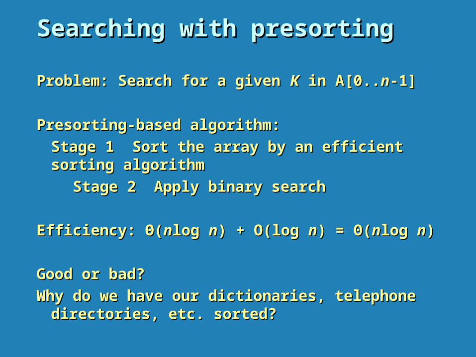
Problem: Search for a given Problem: Search for a given KK in A[0.. in A[0..nn-1]-1]

Presorting-based algorithm:Presorting-based algorithm:

Stage 1 Sort the array by an efficient sorting algorithmStage 1 Sort the array by an efficient sorting algorithm

Stage 2 Apply binary search Stage 2 Apply binary search

Efficiency: Efficiency: ΘΘ((nnlog log nn) + O(log ) + O(log nn) = ) = ΘΘ((nnlog log nn) )

Good or bad?Good or bad?

Why do we have our dictionaries, telephone directories, etc. Why do we have our dictionaries, telephone directories, etc. sorted?sorted?

Element Uniqueness with presortingElement Uniqueness with presorting

Presorting-basedPresorting-based algorithm algorithm Stage 1: sort by efficient sorting algorithm (e.g. mergesort)Stage 1: sort by efficient sorting algorithm (e.g. mergesort)

Stage 2: scan array to check pairs of Stage 2: scan array to check pairs of adjacentadjacent elements elements

EfficiencyEfficiency: : ΘΘ((nnlog log nn) + O() + O(nn) = ) = ΘΘ((nnlog log nn))

Brute force algorithm Brute force algorithm Compare all pairs of elements Compare all pairs of elements

Efficiency: O( Efficiency: O(nn22))

Another algorithm? Another algorithm? • Section 7.3: Using hashing to implement dictionaries.Section 7.3: Using hashing to implement dictionaries.

Instance simplification Instance simplification – Gaussian Elimination– Gaussian Elimination

Given: A system of Given: A system of nn linear equations in linear equations in n n unknowns with an arbitrary unknowns with an arbitrary coefficient matrix.coefficient matrix.

Transform to: An equivalent system of Transform to: An equivalent system of nn linear equations in linear equations in n n unknowns unknowns with an upper triangular coefficient matrix.with an upper triangular coefficient matrix. Solve the latter by substitutions starting with the last equation and moving Solve the latter by substitutions starting with the last equation and moving up to the first one.up to the first one.

aa1111xx1 1 + + aa1212xx2 2 + … + + … + aa11nnxxnn = = b b1 1 aa1,11,1xx11+ + aa1212xx2 2 + … + + … + aa11nnxxnn = = b b11

aa2121xx11 + + aa2222xx2 2 + … + + … + aa22nnxxnn = = b b2 2 aa2222xx2 2 + … + + … + aa22nnxxnn = = b b22

aann11xx11 + + aann22xx2 2 + … + + … + aannnnxxnn = = b bnn aannnnxxnn = = b bnn

Gaussian Elimination (cont.)Gaussian Elimination (cont.)

The transformation is accomplished by a sequence of elementary The transformation is accomplished by a sequence of elementary operations on the system’s coefficient matrix (which don’t operations on the system’s coefficient matrix (which don’t change the system’s solution):change the system’s solution):

forfor i i ←←1 to 1 to n-n-1 1 dodo replace each of the subsequent rows (i.e., rows replace each of the subsequent rows (i.e., rows ii+1, …, +1, …, nn) by ) by a difference between that row and an appropriate multiple a difference between that row and an appropriate multiple of the of the i-i-th row to make the new coefficient in the th row to make the new coefficient in the i-i-thth column column

of that row 0 of that row 0

Example of Gaussian EliminationExample of Gaussian Elimination

Solve 2Solve 2xx11 - 4 - 4xx2 2 + + xx3 3 = 6 = 6 3 3xx11 - - xx2 2 + + xx3 3 = 11= 11 xx11 + + xx2 2 - - xx3 3 = -3= -3

Gaussian eliminationGaussian elimination 22 -4 -4 1 6 2 1 6 2 -4 -4 1 1 6 6 3 -1 1 11 row2 – (3/2)*row1 0 5 -1/2 2 3 -1 1 11 row2 – (3/2)*row1 0 5 -1/2 2 1 1 -1 1 1 -1 -3 row3 – (1/2)*row1 0 3 -3/2 -6 row3–(3/5)*row2-3 row3 – (1/2)*row1 0 3 -3/2 -6 row3–(3/5)*row2

22 -4 -4 1 1 6 6 0 5 -1/2 20 5 -1/2 2 0 0 -6/5 -36/50 0 -6/5 -36/5 Backward substitutionBackward substitution xx33 = (-36/5) / (-6/5) = 6 = (-36/5) / (-6/5) = 6

xx22 = (2+(1/2)*6) / 5 = 1 = (2+(1/2)*6) / 5 = 1

xx11 = (6 – 6 + 4*1)/2 = 2 = (6 – 6 + 4*1)/2 = 2

Pseudocode and Efficiency of Gaussian EliminationPseudocode and Efficiency of Gaussian Elimination

Stage 1: Reduction to the upper-triangular matrixStage 1: Reduction to the upper-triangular matrix

forfor i i ←← 1 1 toto n-n-1 1 dodo

forfor j j ←← ii+1 +1 toto n n dodo for for k k ←← i i toto n+n+1 1 dodo

A A[[jj,, k k] ] ←← AA[[jj,, k k] - ] - AA[[ii,, k k]] * A * A[[jj,, i i] / ] / AA[[ii,, i i] //improve!] //improve!

Stage 2: Backward substitutionStage 2: Backward substitutionforfor j j ←← nn downto downto 1 1 dodo

tt ←← 0 0

forfor k k ←← j j +1+1 toto n n dodo

tt ←← tt + + AA[[jj,, k k] * ] * xx[[kk] ] xx[[jj] ] ←← ( (AA[[jj,, n n+1] - +1] - tt) / ) / AA[[jj,, j j] ]

Efficiency: Efficiency: ΘΘ((nn33)) + + ΘΘ((nn22)) = = ΘΘ((nn33))

Searching ProblemSearching Problem

ProblemProblem: Given a (multi)set : Given a (multi)set S S of keys and a search of keys and a search key key KK, find an occurrence of , find an occurrence of KK in in SS, if any, if any

Searching must be considered in the context of:Searching must be considered in the context of:

• file size (internal vs. external)file size (internal vs. external)

• dynamics of data (static vs. dynamic)dynamics of data (static vs. dynamic)

Dictionary operations (dynamic data):Dictionary operations (dynamic data):

• find (search)find (search)

• insertinsert

• deletedelete

Taxonomy of Searching AlgorithmsTaxonomy of Searching Algorithms List searchingList searching

• sequential searchsequential search• binary searchbinary search• interpolation searchinterpolation search

Tree searching Tree searching • binary search treebinary search tree• binary balanced trees: AVL trees, red-black treesbinary balanced trees: AVL trees, red-black trees• multiway balanced trees: 2-3 trees, 2-3-4 trees, B treesmultiway balanced trees: 2-3 trees, 2-3-4 trees, B trees

HashingHashing• open hashing (separate chaining)open hashing (separate chaining)• closed hashing (open addressing)closed hashing (open addressing)

Binary Search TreeBinary Search Tree

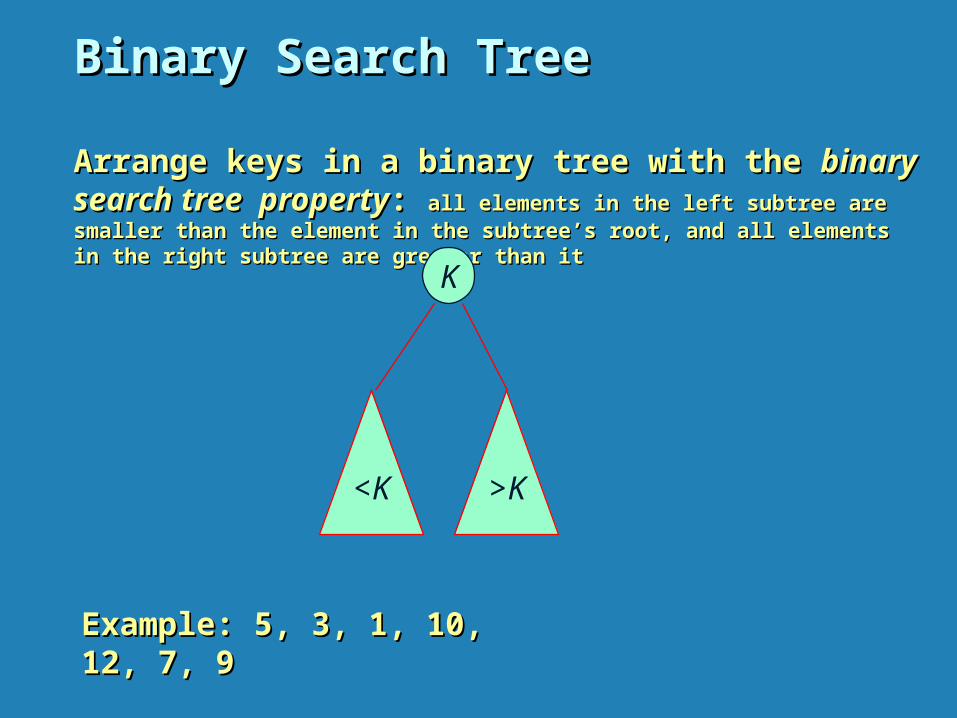
Arrange keys in a binary tree with the Arrange keys in a binary tree with the binary search tree binary search tree propertyproperty: : all elements in the left subtree are smaller than the element in the subtree’s all elements in the left subtree are smaller than the element in the subtree’s root, and all elements in the right subtree are greater than itroot, and all elements in the right subtree are greater than it

K

<K >K

Example: 5, 3, 1, 10, 12, 7, 9Example: 5, 3, 1, 10, 12, 7, 9

Dictionary Operations on Binary Search TreesDictionary Operations on Binary Search Trees

Searching – straightforwardSearching – straightforwardInsertion – search for key, insert at leaf where search terminatedInsertion – search for key, insert at leaf where search terminatedDeletion – 3 cases:Deletion – 3 cases:

deleting key at a leafdeleting key at a leafdeleting key at node with single childdeleting key at node with single childdeleting key at node with two childrendeleting key at node with two children

Efficiency depends of the tree’s height: Efficiency depends of the tree’s height: loglog2 2 nn hh nn-1,-1, with height average (random files) be about 3with height average (random files) be about 3loglog2 2 nn

Thus all three operations haveThus all three operations have• worst case efficiency: worst case efficiency: ((nn) ) • average case efficiency: average case efficiency: (log (log nn) )

BonusBonus: inorder traversal produces sorted list: inorder traversal produces sorted list

Balanced Search Trees Balanced Search Trees

Attractiveness of Attractiveness of binary search tree binary search tree is marred by the bad (linear) is marred by the bad (linear) worst-case efficiency. Two ideas to overcome it are:worst-case efficiency. Two ideas to overcome it are:

to rebalance binary search tree when a new insertionto rebalance binary search tree when a new insertion makes the tree “too unbalanced” makes the tree “too unbalanced”

• AVL treesAVL trees

• red-black treesred-black trees

to allow more than one key per node of a search treeto allow more than one key per node of a search tree

• 2-3 trees2-3 trees

• 2-3-4 trees2-3-4 trees• B-treesB-trees

Balanced trees: AVL treesBalanced trees: AVL trees

DefinitionDefinition An An AVL treeAVL tree is a binary search tree in which, for is a binary search tree in which, for every node, the difference between the heights of its left and every node, the difference between the heights of its left and right subtrees, called the right subtrees, called the balance factorbalance factor, is at most 1 (with , is at most 1 (with the height of an empty tree defined as -1)the height of an empty tree defined as -1)

5 20

124 7

2

(a)

10

1

8

10

1

0

-1

0

0

5 20

4 7

2

(b)

10

2

8

00

1

0

-1

0

Tree (a) is an AVL tree; tree (b) is not an AVL treeTree (a) is an AVL tree; tree (b) is not an AVL tree

RotationsRotations

If a key insertion violates the balance requirement at some If a key insertion violates the balance requirement at some node, the subtree rooted at that node is transformed via one of node, the subtree rooted at that node is transformed via one of the four the four rotations. rotations. (The rotation is always performed for a (The rotation is always performed for a subtree rooted at an “unbalanced” node closest to the new leaf.)subtree rooted at an “unbalanced” node closest to the new leaf.)

3

2

2

1

1

0

2

0

1

0

3

0

>R

(a)

3

2

1

-1

2

0

2

0

1

0

3

0

>LR

(c)

Single Single R-R-rotationrotation Double Double LR-LR-rotationrotation

General case: Single R-rotationGeneral case: Single R-rotation

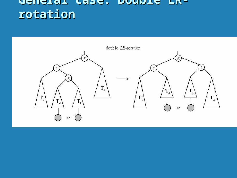
General case: Double LR-rotationGeneral case: Double LR-rotation

AVL tree construction - an exampleAVL tree construction - an example

Construct an AVL tree for the list 5, 6, 8, 3, 2, 4, 7 Construct an AVL tree for the list 5, 6, 8, 3, 2, 4, 7

5

-1

6

0

5

0

5

-2

6

-1

8

0

>6

0

8

0

5

0

L(5)

6

1

5

1

3

0

8

0

6

2

5

2

3

1

2

0

8

0

>R (5)

6

1

3

0

2

0

8

0

5

0

AVL tree construction - an example (cont.)AVL tree construction - an example (cont.)

6

2

3

-1

2

0

5

1

4

0

8

0

>LR (6)

5

0

3

0

2

0

4

0

6

-1

8

0

5

-1

3

0

2

0

4

0

6

-2

8

1

7

0

>RL (6)

5

0

3

0

2

0

4

0

7

0

8

0

6

0

Analysis of AVL treesAnalysis of AVL trees

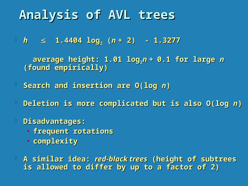
hh 1.4404 1.4404 loglog22 ( (n n + 2) - 1.3277 + 2) - 1.3277

average height: 1.01 average height: 1.01 loglog22n n + + 0.1 for large 0.1 for large n n (found empirically)(found empirically)

Search and insertion are O(Search and insertion are O(log log nn) )

Deletion is more complicated but is also O(Deletion is more complicated but is also O(log log nn))

Disadvantages: Disadvantages: • frequent rotationsfrequent rotations• complexitycomplexity

A similar idea: A similar idea: red-black treesred-black trees (height of subtrees is allowed to (height of subtrees is allowed to differ by up to a factor of 2) differ by up to a factor of 2)

Multiway Search TreesMultiway Search Trees

DefinitionDefinition A A multiway search treemultiway search tree is a search tree that allows is a search tree that allowsmore than one key in the same node of the tree.more than one key in the same node of the tree.

DefinitionDefinition A node of a search tree is called an A node of a search tree is called an nn--nodenode if it contains if it contains n-n-1 1 ordered keys (which divide the entire key range into ordered keys (which divide the entire key range into nn intervals pointed to intervals pointed to by the node’s by the node’s n n links to its children):links to its children):

Note: Every node in a classical binary search tree is a 2-nodeNote: Every node in a classical binary search tree is a 2-node

k1 < k2 < … < kn-1

< k1 [k1, k2 ) kn-1

2-3 Tree 2-3 Tree

DefinitionDefinition A A 2-3 tree2-3 tree is a search tree that is a search tree that may have 2-nodes and 3-nodesmay have 2-nodes and 3-nodes height-balanced (all leaves are on the same level)height-balanced (all leaves are on the same level)

A 2-3 tree is constructed by successive insertions of keys given, with a A 2-3 tree is constructed by successive insertions of keys given, with a new key always inserted into a leaf of the tree. If the leaf is a 3-node, new key always inserted into a leaf of the tree. If the leaf is a 3-node, it’s split into two with the middle key promoted to the parent.it’s split into two with the middle key promoted to the parent.

K K , K1 2

(K , K )1 2

2-node 3-node

< K > K< K > K 1 2

2-3 tree construction – an example2-3 tree construction – an example

Construct a 2-3 tree the list 9, 5, 8, 3, 2, 4, 7Construct a 2-3 tree the list 9, 5, 8, 3, 2, 4, 7

9>

8

955, 9 5, 8, 9

8

93, 5

2, 3, 5

8

9

>

>

3, 8

92 5

3, 8

92 4, 5

3, 8

4, 5, 72 9

> 3, 5, 8

2 4 7 9

5

3

42

8

97

Analysis of 2-3 treesAnalysis of 2-3 trees

loglog3 3 ((n n + 1) - 1 + 1) - 1 hh loglog22 ( (n n + 1) - 1+ 1) - 1

Search, insertion, and deletion are in Search, insertion, and deletion are in ((log log nn) )

The idea of 2-3 tree can be generalized by allowing more The idea of 2-3 tree can be generalized by allowing more keys per node keys per node

• 2-3-4 trees 2-3-4 trees

• B-treesB-trees

Heaps and HeapsortHeaps and Heapsort

DefinitionDefinition A A heapheap is a binary tree with keys at its nodes (one is a binary tree with keys at its nodes (one key per node) such that:key per node) such that:

It is essentially complete, i.e., all its levels are full except It is essentially complete, i.e., all its levels are full except possibly the last level, where only some rightmost keys may possibly the last level, where only some rightmost keys may be missingbe missing

The key at each node is The key at each node is ≥≥ keys at its children keys at its children • Automatically satisfied for all leavesAutomatically satisfied for all leaves

• min-heap – this makes more sense to memin-heap – this makes more sense to me

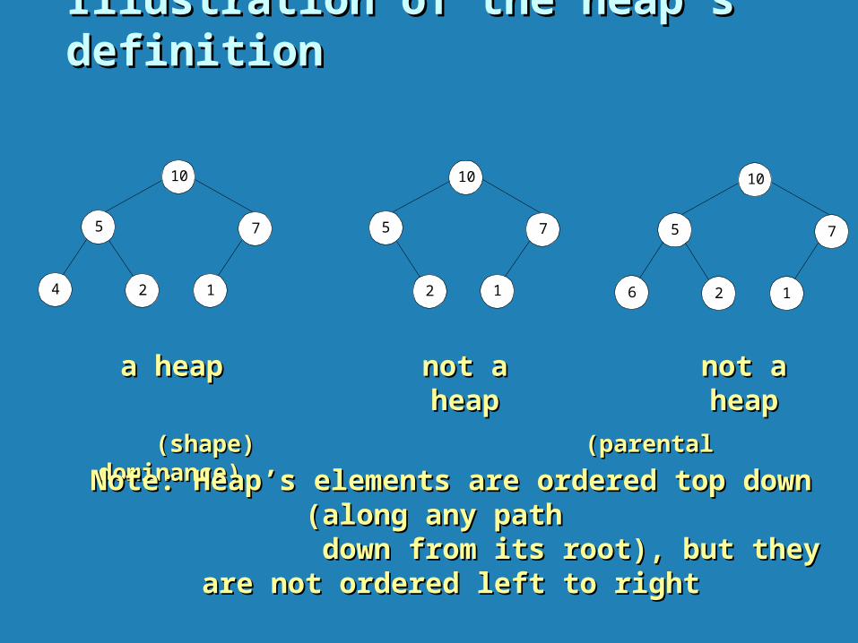
Illustration of the heap’s definitionIllustration of the heap’s definition

(shape) (parental (shape) (parental dominance)dominance)

10

5

4 2

7

1

10

5

2

7

1

10

5

6 2

7

1

a heapa heap not a heapnot a heap not a heapnot a heap

Note: Heap’s elements are ordered top down (along any path Note: Heap’s elements are ordered top down (along any path down from its root), but they are not ordered left to right down from its root), but they are not ordered left to right

Some Important Properties of a HeapSome Important Properties of a Heap

Page 224 - Page 224 - see Figure 6.10 and next slidesee Figure 6.10 and next slide

Given Given n,n, there exists a unique binary tree with there exists a unique binary tree with nn nodes that nodes that

is essentially complete, with is essentially complete, with h h = = loglog2 2 nn

The root contains the largest keyThe root contains the largest key• I like the smallest myselfI like the smallest myself

The subtree rooted at any node of a heap is also a heapThe subtree rooted at any node of a heap is also a heap

A heap can be represented as an arrayA heap can be represented as an array

Heap’s Array RepresentationHeap’s Array Representation

Store heap’s elements in an array (whose elements indexed, Store heap’s elements in an array (whose elements indexed, for convenience, 1 to for convenience, 1 to nn) in top-down left-to-right order) in top-down left-to-right order

Example:Example:

Left child of node Left child of node jj is at 2 is at 2jj Right child of node Right child of node jj is at 2 is at 2jj+1+1 Parent of node Parent of node jj is at is at jj/2/2 Parental nodes are represented in the first Parental nodes are represented in the first nn/2/2 locationslocations

9

1

5 3

4 2

1 2 3 4 5 6

9 5 3 1 4 2

Step 0: Initialize the structure with keys in the order givenStep 0: Initialize the structure with keys in the order given

Step 1: Starting with the last (rightmost) parental node, fix Step 1: Starting with the last (rightmost) parental node, fix the heap rooted at it, if it doesn’t satisfy the heap the heap rooted at it, if it doesn’t satisfy the heap condition: keep exchanging it with its largest child condition: keep exchanging it with its largest child

until the heapuntil the heap condition holdscondition holds

Step 2: Repeat Step 1 for the preceding parental nodeStep 2: Repeat Step 1 for the preceding parental node

Heap Construction (bottom-up)Heap Construction (bottom-up)(There is also top-down heap construction – page 226)(There is also top-down heap construction – page 226)

Example of Heap ConstructionExample of Heap Construction

7

2

9

6 5 8

>

2

9

6 5

8

7

2

9

6 5

8

7

2

9

6 5

8

7

>

9

2

6 5

8

7

9

6

2 5

8

7

>

Construct a heap for the list 2, 9, 7, 6, 5, 8Construct a heap for the list 2, 9, 7, 6, 5, 8

Pseudopodia of bottom-up heap constructionPseudopodia of bottom-up heap construction

Insertion of a New Element into a HeapInsertion of a New Element into a Heap

Insert the new element at last position in heap. Insert the new element at last position in heap. Compare it with its parent and, if it violates heap condition,Compare it with its parent and, if it violates heap condition,

exchange themexchange them Continue comparing the new element with nodes up the tree Continue comparing the new element with nodes up the tree

until the heap condition is satisfieduntil the heap condition is satisfied

Example:Example: Insert key 10Insert key 10

Efficiency: O(log Efficiency: O(log nn))

9

6

2 5

8

7 10

9

6

2 5

10

7 8

> >

10

6

2 5

9

7 8

Stage 1: Construct a heap for a given list of Stage 1: Construct a heap for a given list of nn keys keys

Stage 2: Repeat operation of root removal Stage 2: Repeat operation of root removal nn-1 times:-1 times:

– Exchange keys in the root and in the last Exchange keys in the root and in the last (rightmost) leaf(rightmost) leaf

– Decrease heap size by 1Decrease heap size by 1

– If necessary, swap new root with larger child until If necessary, swap new root with larger child until the heap condition holdsthe heap condition holds

HeapsortHeapsort

Sort the list 2, 9, 7, 6, 5, 8 by heapsortSort the list 2, 9, 7, 6, 5, 8 by heapsort

Stage 1 (heap construction)Stage 1 (heap construction) Stage 2 (root/max removal) Stage 2 (root/max removal)

2 9 2 9 77 6 5 8 6 5 8 99 6 8 2 5 7 6 8 2 5 7

2 2 99 8 6 5 7 8 6 5 7 7 6 8 2 5 | 9 7 6 8 2 5 | 9

22 9 8 6 5 7 9 8 6 5 7 88 6 7 2 5 | 9 6 7 2 5 | 9

9 9 22 8 6 5 7 8 6 5 7 5 6 7 2 | 8 9 5 6 7 2 | 8 9

9 6 8 2 5 79 6 8 2 5 7 77 6 5 2 | 8 9 6 5 2 | 8 9

2 6 5 | 7 8 92 6 5 | 7 8 9

66 2 5 | 7 8 9 2 5 | 7 8 9

55 2 | 6 7 8 9 2 | 6 7 8 9

55 2 | 6 7 8 9 2 | 6 7 8 9

2 | 5 6 7 8 92 | 5 6 7 8 9

Example of Sorting by HeapsortExample of Sorting by Heapsort

Stage 1: Build heap for a given list of Stage 1: Build heap for a given list of nn keys keysworst-caseworst-case CC((nn) = ) =

Stage 2: Repeat operation of root removal Stage 2: Repeat operation of root removal nn-1 times (fix heap)-1 times (fix heap)worst-caseworst-case CC((nn) = ) =

Both worst-case and average-case efficiency: Both worst-case and average-case efficiency: ((nnloglognn) ) In-place: yesIn-place: yesStability: no (e.g., 1 1)Stability: no (e.g., 1 1)

2(2(h-ih-i) 2) 2i i = = 2 ( 2 ( nn – log – log22((n n + 1)) + 1)) ((nn))ii=0=0

hh-1-1

# nodes at level i

i=i=11

nn-1-1 2log2log2 2 i i ((nnloglognn))

Analysis of HeapsortAnalysis of Heapsort

A A priority queue priority queue is the ADT of a set of elements with is the ADT of a set of elements with

numerical priorities with the following operations:numerical priorities with the following operations:

• find element with highest priorityfind element with highest priority

• delete element with highest prioritydelete element with highest priority

• insert element with assigned priority (see below)insert element with assigned priority (see below)

Heap is a very efficient way for implementing priority queuesHeap is a very efficient way for implementing priority queues

Two ways to handle priority queue in whichTwo ways to handle priority queue in which highest priority = smallest number highest priority = smallest number

Priority QueuePriority Queue

Horner’s Rule For Polynomial EvaluationHorner’s Rule For Polynomial Evaluation

Given a polynomial of degree Given a polynomial of degree nn

pp((xx) = ) = aannxxnn + a + ann-1-1xxnn-1-1 + … + + … + aa11xx + + aa00

and a specific value of and a specific value of xx, find the value of , find the value of pp at that point. at that point.

Two brute-force algorithms:Two brute-force algorithms:

pp 0 0 pp aa00; ; powerpower 1 1

for for i i nn downto 0downto 0 dodo for for i i 1 to 1 to n n dodo power power 1 1 powerpower powerpower * * xx

for for jj 1 to 1 to ii do do pp pp + + aai i * * powerpower powerpower powerpower * * x x return return pp

pp p + ap + aii * * powerpower

return return pp

Horner’s RuleHorner’s Rule

Example: Example: pp(x) = 2(x) = 2xx44 - - xx33 + 3 + 3xx22 + + xx - 5 = - 5 =

= = xx(2(2xx33 - - xx22 + 3 + 3xx + 1) - 5 = + 1) - 5 =

= = xx((xx(2(2xx22 - - xx + 3) + 1) - 5 = + 3) + 1) - 5 =

= = xx((xx((xx(2(2xx - 1) + 3) + 1) - 5 - 1) + 3) + 1) - 5

Substitution into the last formula leads to a faster algorithm Substitution into the last formula leads to a faster algorithm

Same sequence of computations are obtained by simply Same sequence of computations are obtained by simply arranging the coefficient in a table and proceeding as follows: arranging the coefficient in a table and proceeding as follows:

coefficientscoefficients 22 -1-1 3 3 1 1 -5-5

xx=3=3

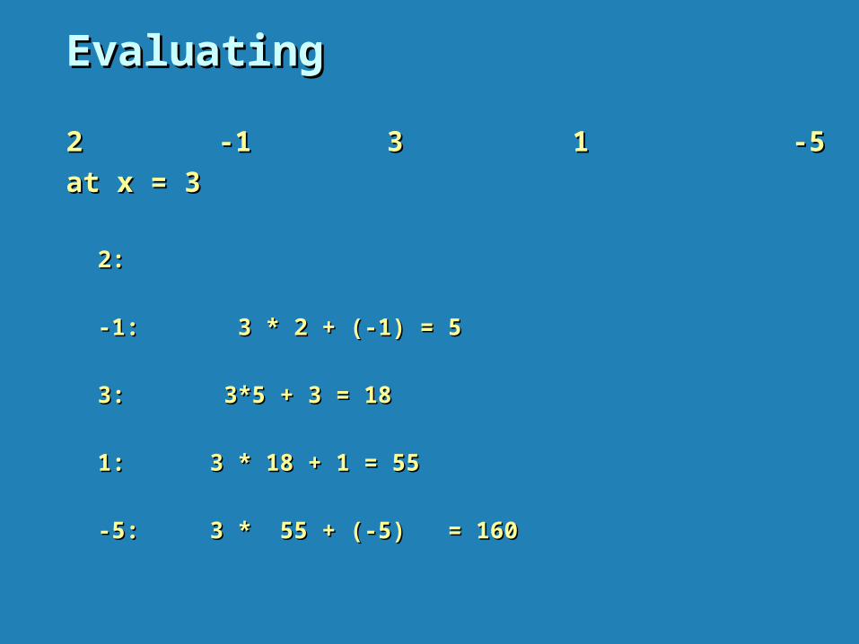
EvaluatingEvaluating

2 -1 3 1 -52 -1 3 1 -5

at x = 3at x = 3

2: 2:

-1: 3 * 2 + (-1) = 5-1: 3 * 2 + (-1) = 5

3: 3*5 + 3 = 183: 3*5 + 3 = 18

1: 3 * 18 + 1 = 551: 3 * 18 + 1 = 55

-5: 3 * 55 + (-5) = 160-5: 3 * 55 + (-5) = 160

Horner’s Rule pseudocodeHorner’s Rule pseudocode

Efficiency of Horner’s Rule: # multiplications = # additions = Efficiency of Horner’s Rule: # multiplications = # additions = nn

Synthetic division is byproduct of HornerSynthetic division is byproduct of Horner

SSynthetic divisionynthetic division of of pp((xx) by () by (x-xx-x00) )

Example: Let Example: Let pp((xx) = 2) = 2xx44 - - xx33 + 3 + 3xx22 + + x x - 5. Find - 5. Find pp((xx):():(xx-3)-3)

The intermediate numbers generated by the algorithm in The intermediate numbers generated by the algorithm in the process of evaluating p(x) at some point xthe process of evaluating p(x) at some point x00 turn out to turn out to

be the coefficients of the quotient of the division of p(x) by x be the coefficients of the quotient of the division of p(x) by x - x- x0 0

Do we get in the previous example the following quotient Do we get in the previous example the following quotient 2x2x33 + 5x + 5x22 +18x + 55 +18x + 55

Computing Computing aann (revisited) (revisited)

Left-to-right binary exponentiationLeft-to-right binary exponentiation Initialize product accumulatorInitialize product accumulator by 1.by 1.Scan Scan nn’s binary expansion from left to right and do the ’s binary expansion from left to right and do the following: following: If the current binary digit is 0, square the accumulator (S);If the current binary digit is 0, square the accumulator (S);if the binary digit is 1, square the accumulator and multiply it if the binary digit is 1, square the accumulator and multiply it by by a a (SM).(SM).

Example: Compute aExample: Compute a1313. Here, . Here, nn = 13 = 1101 = 13 = 110122. . binary rep. of 13: 1 1binary rep. of 13: 1 1 0 1 0 1

SM SM SM SM S S SM SM accumulator: 1 1accumulator: 1 122**a=aa=a aa22**aa = = aa33 ( (aa33))22 = = aa66 ( (aa66))22**aa= = aa13 13 (computed left-to-right)(computed left-to-right)

Efficiency: (Efficiency: (b-b-1) 1) ≤≤ M( M(nn) ) ≤≤ 2 2((b-b-1) where 1) where b = b = loglog2 2 nn + 1 + 1

Computing Computing aann (cont.) (cont.)

Right-to-left binary exponentiationRight-to-left binary exponentiation

Scan Scan nn’s binary expansion from right to left and compute ’s binary expansion from right to left and compute aann as as the product of terms the product of terms aa2 2 ii corresponding to 1’s in this expansion. corresponding to 1’s in this expansion.

ExampleExample Compute Compute aa13 13 by the right-to-left binary exponentiation. by the right-to-left binary exponentiation. Here, Here, nn = 13 = 1101 = 13 = 110122. .

11 1 1 0 1 0 1 a a88 a a44 a a22 a a : : aa2 2 ii terms terms a a88 * a * a44 * a * a : product : product (computed right-to-left) (computed right-to-left)

Efficiency: same as that of left-to-right binary exponentiationEfficiency: same as that of left-to-right binary exponentiation

Problem ReductionProblem Reduction

This variation of transform-and-conquer solves a problem by This variation of transform-and-conquer solves a problem by a transforming it into different problem for which an a transforming it into different problem for which an algorithm is already available.algorithm is already available.

To be of practical value, the combined time of the To be of practical value, the combined time of the transformation and solving the other problem should be transformation and solving the other problem should be smaller than solving the problem as given by another smaller than solving the problem as given by another method. method.

Examples of Solving Problems by ReductionExamples of Solving Problems by Reduction

computing lcm(computing lcm(mm, , nn) via computing gcd() via computing gcd(m, nm, n))

lcm(m,n) = m*n / gcd(m,n)lcm(m,n) = m*n / gcd(m,n)• has improvement since Euclid’s algorithm is fast.has improvement since Euclid’s algorithm is fast.

counting number of paths of length counting number of paths of length n n in a graph by raising in a graph by raising the graph’s adjacency matrix to the the graph’s adjacency matrix to the n-n-th powerth power

transforming a maximization problem to a minimization transforming a maximization problem to a minimization problem and vice versa (also, min-heap construction)problem and vice versa (also, min-heap construction)

Problem Reduction (2)Problem Reduction (2)

linear programminglinear programming

reduction to graph problems (e.g., solving puzzles via state-reduction to graph problems (e.g., solving puzzles via state-space graphs) space graphs)