1

Chapter 5: Chapter 5: Factorial designs

Petter Mostadmostad@chalmers.semostad@chalmers.se

Experiments• Actively making changes and observing the result, • Actively making changes and observing the result,

to find causal relationships. • Many types of experimental plans

– Measuring response over a range of values– Searching for factors influencing a result– …

• Make sure experiment is likely to answer your • Make sure experiment is likely to answer your questions. Adapt the experiment to the questionyou want to ask!

2

Factorial designs• A number of factors are selected: They can be set by the • A number of factors are selected: They can be set by the

experimenter, and they are suspected to influence the measured outcome

• Two or more levels are selected for each factor. • The experiment is performed using all combinations of all

factor levels• The experiment may be replicated n times for each • The experiment may be replicated n times for each

combination of factor levels. • All other factors, including time should be randomized!

Why use factorial designs?

• Efficient way to estimate the effect of • Efficient way to estimate the effect of varying the factors

• Effect is estimated averaged over other factors

• Interaction effects may be detected• Computations are simple (with equal

number of replications for each setting)

3

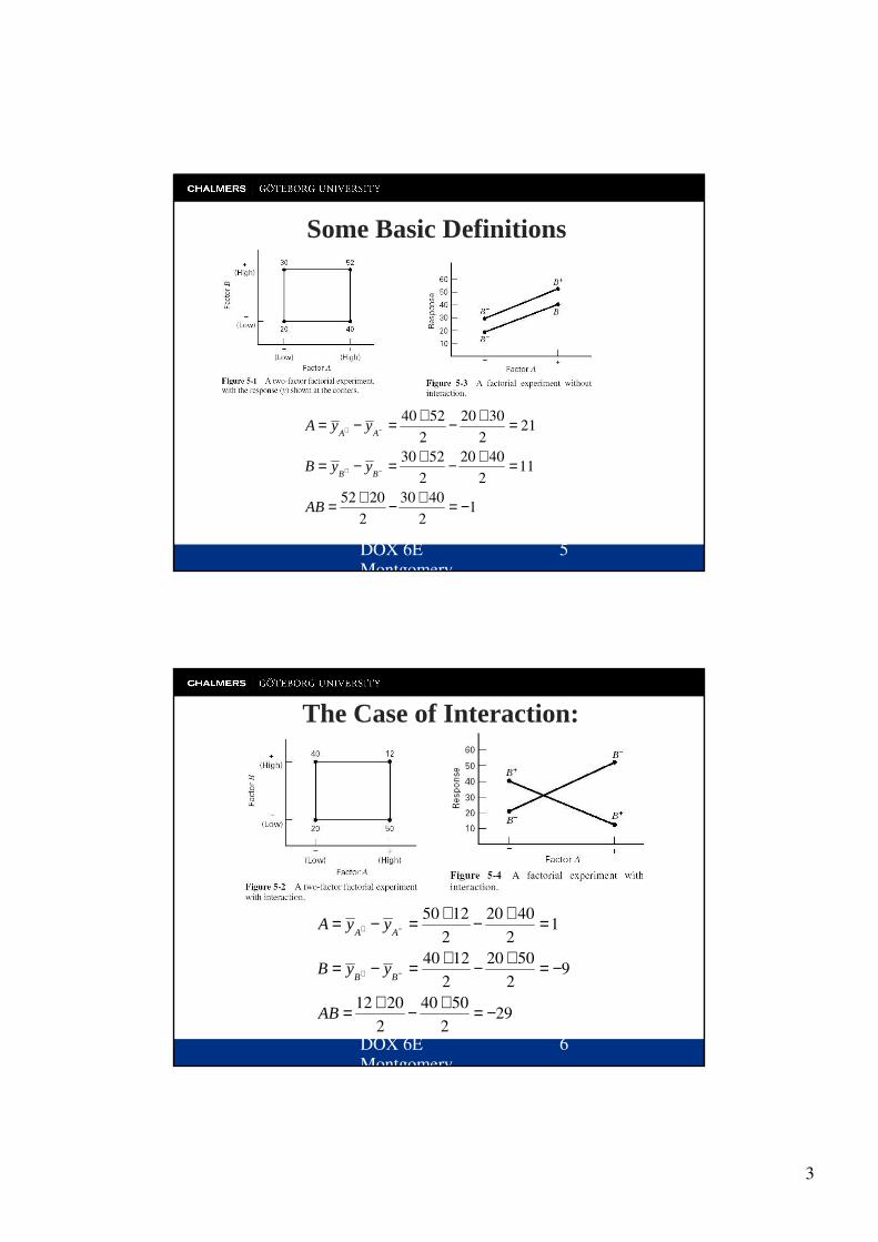
Some Basic Definitions

Definition of a factor effect: The change in the mean response when the factor is changed from low to high40 52 20 30 21

2 2A AA y y+ −

+ += − = − =

DOX 6E Montgomery

5

2 230 52 20 40 11

2 252 20 30 40 1

2 2

B BB y y

AB

+ −

+ += − = − =

+ += − = −

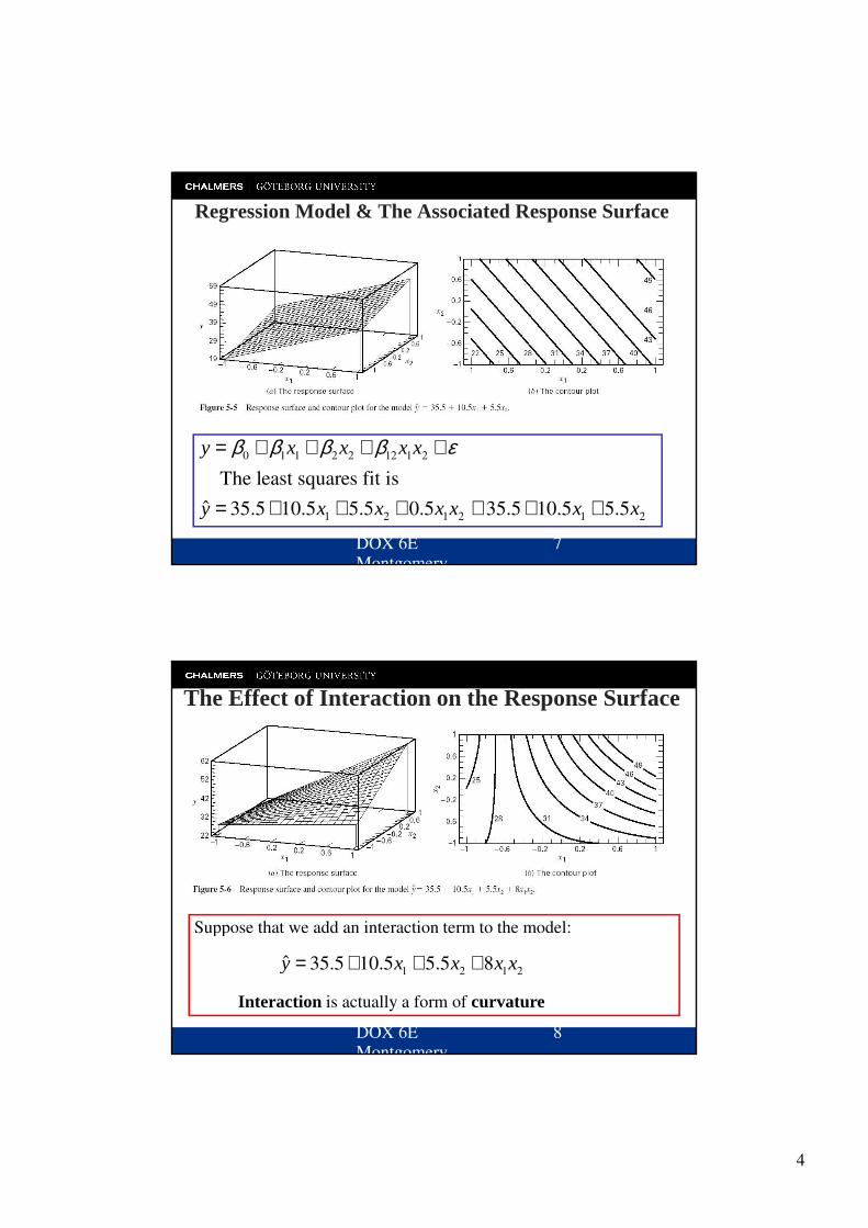
The Case of Interaction:

50 12 20 40 12 2A A

A y y+ −

+ += − = − =

DOX 6E Montgomery

6

2 240 12 20 50 9

2 212 20 40 50 29

2 2

A A

B BB y y

AB

+ −

+ += − = − = −

+ += − = −

4

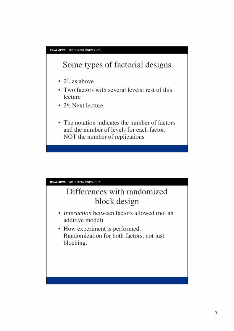
Regression Model & The Associated Response Sur face

DOX 6E Montgomery

7

0 1 1 2 2 12 1 2

1 2 1 2 1 2

The least squares fit isˆ 35.5 10.5 5.5 0.5 35.5 10.5 5.5

y x x x x

y x x x x x x

β β β β ε= + + + +

= + + + ≅ + +

The Effect of Interaction on the Response Sur face

Suppose that we add an interaction term to the model:

DOX 6E Montgomery

8

Suppose that we add an interaction term to the model:

1 2 1 2ˆ 35.5 10.5 5.5 8y x x x x= + + +

Interaction is actually a form of curvature

5

Some types of factorial designs

• 22, as above• 22, as above• Two factors with several levels: rest of this

lecture• 2k: Next lecture

• The notation indicates the number of factors and the number of levels for each factor, NOT the number of replications

Differences with randomized block design

• Interaction between factors allowed (not an • Interaction between factors allowed (not an additive model)

• How experiment is performed: Randomization for both factors, not just blocking.

6

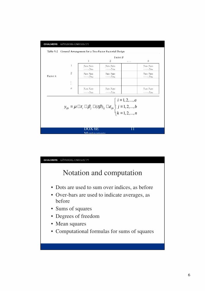
Statistical (effects) model:1, 2,...,i a=�

�

DOX 6E Montgomery

11

( ) 1,2,...,1, 2,...,

ijk i j ij ijky j b

k n

µ τ β τβ ε �= + + + + =�� =�

Other models (means model, regression models) can be useful

Notation and computation

• Dots are used to sum over indices, as before• Dots are used to sum over indices, as before• Over-bars are used to indicate averages, as

before• Sums of squares• Degrees of freedom• Degrees of freedom• Mean squares• Computational formulas for sums of squares

7

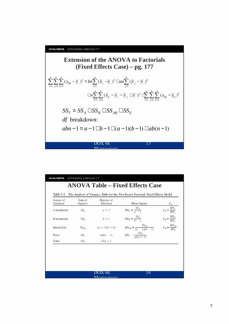
Extension of the ANOVA to Factor ials (Fixed Effects Case) – pg. 177

2 2 2( ) ( ) ( )a b n a b

y y bn y y an y y− = − + −� � � � �2 2 2... .. ... . . ...

1 1 1 1 1

2 2. .. . . ... .

1 1 1 1 1

( ) ( ) ( )

( ) ( )

ijk i ji j k i j

a b a b n

ij i j ijk iji j i j k

y y bn y y an y y

n y y y y y y

= = = = =

= = = = =

− = − + −

+ − − + + −

� � � � �

� � � � �

T A B AB ESS SS SS SS SS= + + +

DOX 6E Montgomery

13

breakdown:1 1 1 ( 1)( 1) ( 1)

T A B AB E

df

abn a b a b ab n− = − + − + − − + −

ANOVA Table – Fixed Effects Case

DOX 6E Montgomery

14

8

Hypothesis testing

• Normality assumptions about the • Normality assumptions about the observations in each group

• Three different null hypotheses: No interaction, no row effect, no column effect.

• The distribution of the test statistic under the null hypothesis. the null hypothesis.

Checking assumptions

• Compute the residuals! • Compute the residuals! • Plot the residuals in various ways• Check also the random sample assumption

9

Example 5-1 The Battery L ife Exper imentText reference pg. 165

DOX 6E Montgomery

17

Design and Analysis of Experiments, 6/Eby Douglas C. Montgomery

Table 5.5 (p. 170)Analysis of Variance for Battery Life Data

10

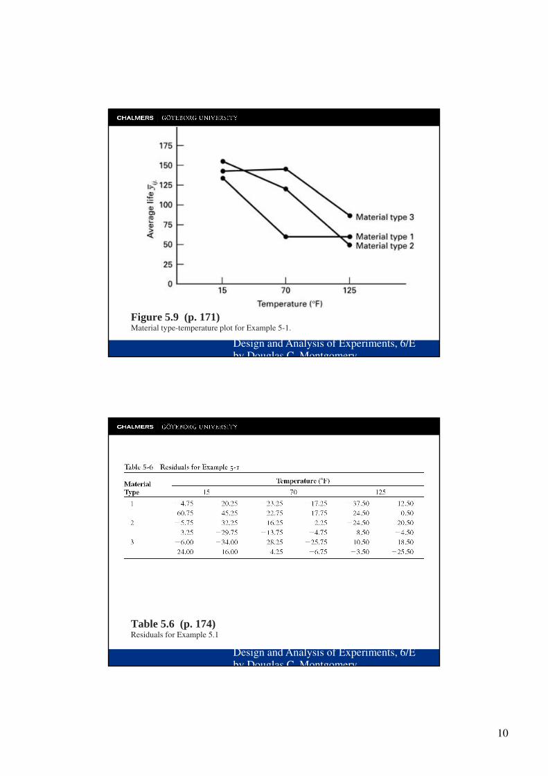
Design and Analysis of Experiments, 6/Eby Douglas C. Montgomery

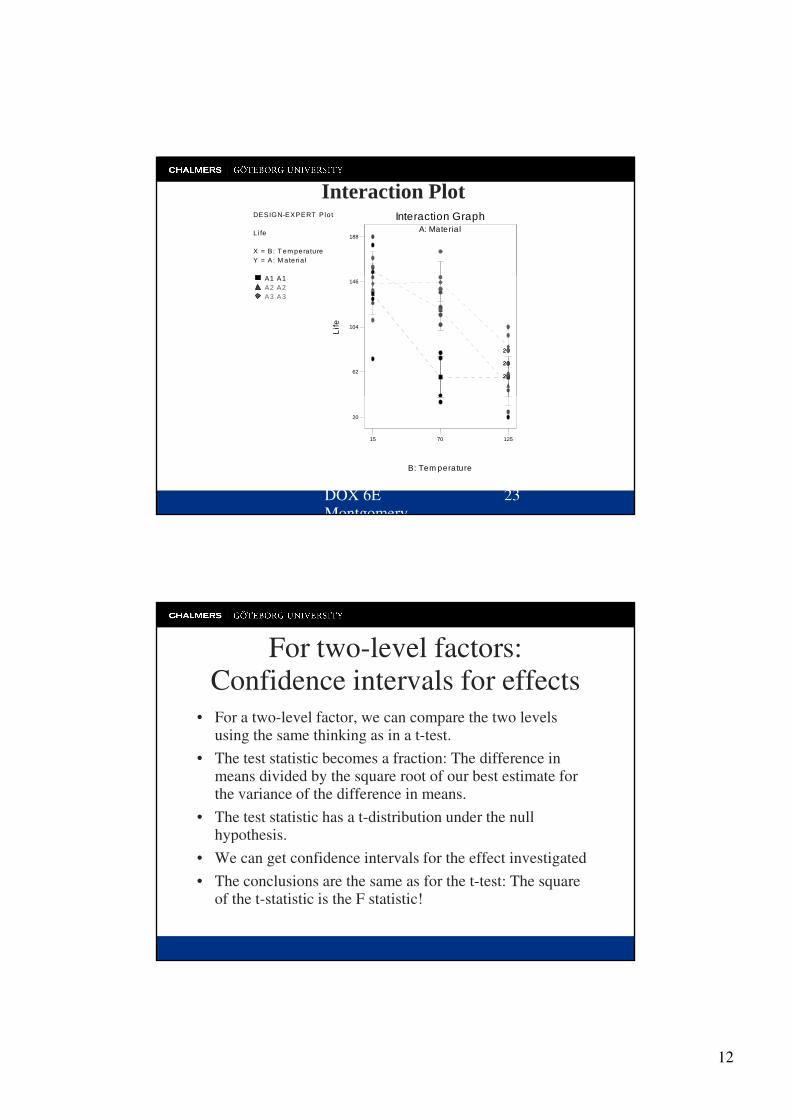
Figure 5.9 (p. 171)Material type-temperature plot for Example 5-1.

Design and Analysis of Experiments, 6/Eby Douglas C. Montgomery

Table 5.6 (p. 174)Residuals for Example 5.1

11

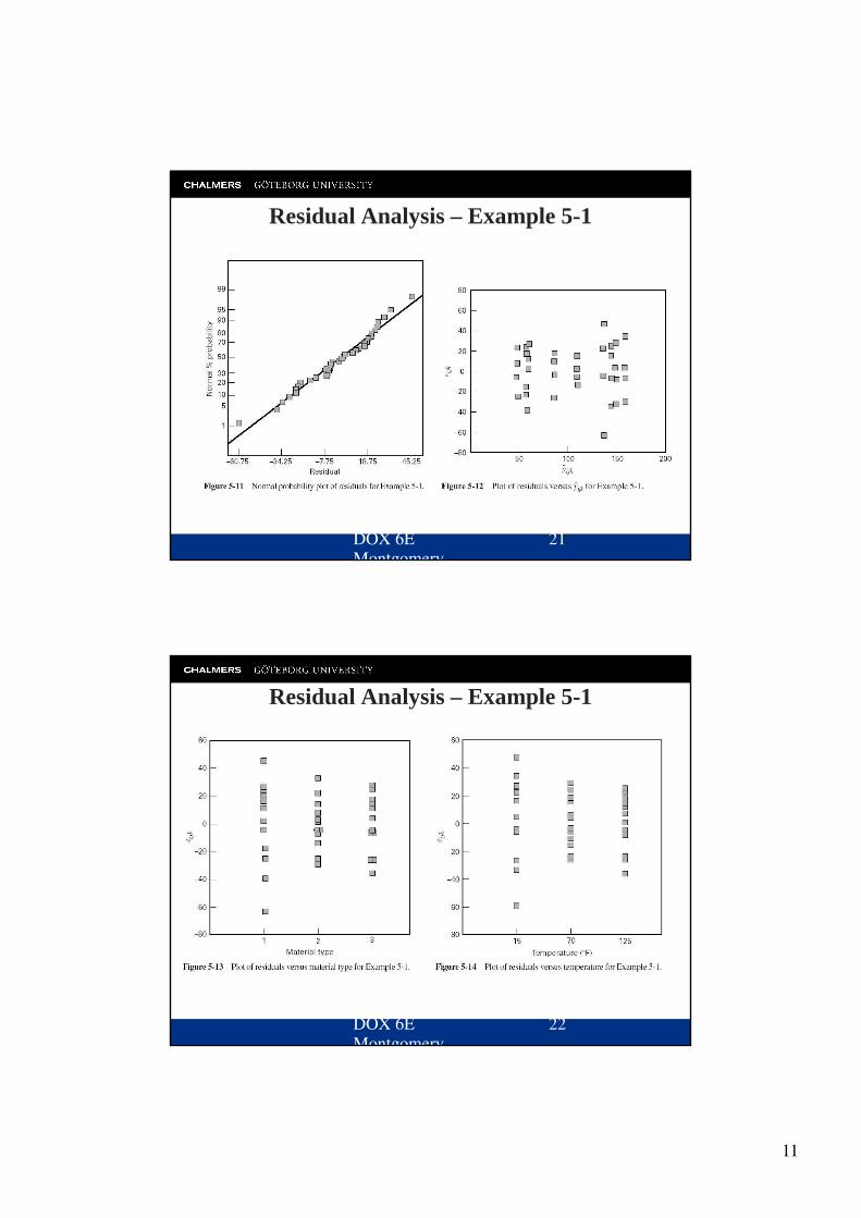
Residual Analysis – Example 5-1

DOX 6E Montgomery

21

Residual Analysis – Example 5-1

DOX 6E Montgomery

22

12

Interaction Plot DESIGN-EXPERT P lo t

L i fe

X = B: T em peratureY = A: M ateria l

A1 A1

A: Materia l

Interaction Graph

188

A1 A1A2 A2A3 A3

Life

62

104

146

2

2

22

2

2

DOX 6E Montgomery

23

B: Tem perature

15 70 125

20

For two-level factors: Confidence intervals for effects

• For a two-level factor, we can compare the two levels• For a two-level factor, we can compare the two levelsusing the same thinking as in a t-test.

• The test statistic becomes a fraction: The difference in means divided by the square root of our best estimate for the variance of the difference in means.

• The test statistic has a t-distribution under the nullhypothesis. hypothesis.

• We can get confidence intervals for the effect investigated• The conclusions are the same as for the t-test: The square

of the t-statistic is the F statistic!

13

What to test, and conclusions• Test first whether there is an interaction• Test first whether there is an interaction• If there is an interaction, the effects of rows and columns

may be difficult to interpret by themselves• If you get a high p-value when testing for interaction, it

may be a good idea to use a model without interaction (as in the randomized blocks computations)

• NOTE: Results from a model without interaction can be • NOTE: Results from a model without interaction can be seen directly from the ANOVA table!

One observation per cell

• With only one observation per cell, it is • With only one observation per cell, it is impossible to test whether there is interaction or not: Too few degrees of freedom!

• One approach: Fit a model withoutinteraction, and study the residuals to interaction, and study the residuals to determine if you believe there is interaction or not.

14

Making concludions, multiple testing, and Tukey’s procedure

• Once you have your model (interaction or • Once you have your model (interaction or not) you will want to find which effects are significantly different, and which are not.

• You can make pairwise tests, or computeconfidence intervals for differences, as above. above.

• Multiple testing is an issue: One way to deal with this is Tukey’s procedure.

Overview

• Given data from factorial experiment: How to • Given data from factorial experiment: How to analyze? – Plot data– If only one observation per cell, compute the

interaction, or assume no interaction and look at the residuals

– Otherwise, test for an interaction term– Otherwise, test for an interaction term– Estimate the effects in the chosen model– Study residuals! Check the model– Find conf. intervals, possibly with Tukey’s method