100

Chapter 5. Determinants of Economic-BasedProtection from Technical Barriers to U.S.Agricultural Exports

5.1. Introduction

Despite the efforts of the international trading community to limit misuse of technicalbarriers through the Uruguay Round Agreements, the 1996 USDA Survey results suggest thatthese regulatory measures continue to provide disguised economic-based protection for domesticindustries. Political economy is a paradigm that explains government intervention in the market,where policy choice is endogenously determined by individual agents and policymakers acting asrational maximizers given their sets of preferences. The interaction between economics andpolitics may result in policies which are net welfare decreasing, such as the provision ofeconomic-based protection through technical barriers.

Empirical models quantify the economic and political incentives and abilities ofindividual agents and policymakers to affect regulatory outcomes. An empirical approach similarto those used in previous studies of other trade and agricultural policy decisions can be applied toanalyze the political economy factors underlying the incidence and impact of questionabletechnical barriers. In this chapter, two fundamental empirical models are exposited to identifythe determinants of economic-based protection from questionable technical barriers as they areapplied to U.S. agricultural exports. The purpose of the empirical models is not to test thepolitical economy theory, but rather to identify the common factors underlying observedregulatory levels and to quantify the economic and political relationships that give rise toquestionable technical barriers.

The first model addresses the incidence of questionable barriers. The dependent variablein this model measures the presence or absence of questionable technical barriers applied bycountry. The second empirical model addresses the impact of questionable technical barriers.The dependent variable measures the estimated trade impact from questionable technical barriersas a percentage of 1996 U.S. agricultural exports to that country. For each of these two models anumber of econometric specifications are estimated.

Independent variables in the econometric models represent the influence of market andpolitical economy factors, as well as the possible influence of survey design characteristics on theestimation results. The variables reflect influential measures identified in the theoretical andempirical political economy models discussed in Chapter Three including characteristics of trade,agriculture, and the aggregate economy. Such a characterization can then be reorganized to

101

provide proxy measures for the interests of individual agents, effective political influence,policymaker preferences, and institutional structures, as depicted in Figure 3.3.

Section 5.2 introduces the dependent and independent variables used in the econometricestimations to represent the political economy of technical barriers. A univariate PROBIT modelthat quantifies the incidence of questionable technical barriers is presented in Section 5.3 wherethe dependent variable is a binary representation of the presence or absence of questionabletechnical barriers by country. Section 5.4 presents a TOBIT model to measure the impact ofquestionable technical barriers. The dependent variable measures the estimated percentagerevenue loss from questionable technical barriers, distributed continuously and censored at zero.A summary and conclusions are presented in Section 5.5.

5.2. Econometric Models of Questionable Technical Barriers to U.S.Agricultural Exports

The political economy theory presented in Chapter Three provides a conceptualframework for empirical analysis of the economic-based protection provided by questionabletechnical barriers. This is the underlying theoretical paradigm represented in the followingempirical models. An approach similar to those used to model other agricultural and trade policydecisions is applied to analyze the reported incidence and impact of questionable technicalbarriers. Since individual agent preferences, effective political influence, policymakerpreferences, and institutional structures cannot be measured directly, a number of variables arespecified as proxy measures for the underlying political economy relationships. Taken together,the set of independent variables selected for inclusion in the models gives a broadcharacterization of the likely political economy influences on the regulatory decisions.

5.2.a. Measures of Incidence and Impact

The incidence and impact of questionable technical barriers to U.S. agricultural exports,as presented in Chapter Four, provides measures of potential economic-based protection on across-sectional basis at one point in time. There are several ways to quantify protection usingthis data. The presence or absence of barriers identified as questionable reflects the incidence ofprotection, while the percentage estimated trade impact reflects the impact of protection.

5.2.a.1. Presence of Questionable Technical Barriers

The presence or absence of questionable technical barriers includes all observations in the1996 USDA Survey summed by country (n=134). This is a binary variable, YN, where one isused to indicate the presence of one or more questionable technical barriers to U.S. agriculturalexports and zero is used to indicate the absence of such barriers. There are 63 one-observations

102

and 71 zero-observations of the YN variable included in the sample (see Appendix B for a list ofcountries included in each category).

5.2.a.2. Percentage Trade Impact from Questionable Technical Barriers

The impact of questionable technical barriers applied to U.S. agricultural exports ismeasured in the 1996 USDA Survey by the estimated loss, or potential loss, in 1996 exportrevenues attributable to these barriers assuming a fixed world price. To correct for magnitudedifferences in trade among countries and commodities it is useful to normalize the estimatedtrade impact values from the survey. This is a censored normal variable, PETI, where percentageimpact is measured as the estimated trade impact (from the 1996 USDA Survey) divided by thetotal value of 1996 U.S. agricultural exports to the country imposing the barrier. Again,observations are summed by countries (n = 134). Values range from zero, for those 71 countrieswhere no questionable technical barriers were identified, to 412, where the estimated tradeimpact from technical barriers in 1996 was large relative to total 1996 agricultural exports to thatcountry. In the previous chapter, Table 4.28 shows a distribution of countries in the sample bythe percentage estimated trade impact.

5.2.b. Measures of the Political Economy Determinants of Questionable Technical Barriers

Following the approach used in the empirical studies reviewed in Chapter Three, anumber of independent variables are identified to serve as proxies for the political economydeterminants of questionable technical barriers due, in part, to the fallibility of particular singlemeasures (Bollen 1980; Beghin and Kherallah 1994). Since the measures of incidence andimpact of economic-based protection represent cross-country observations, the independentvariables in the econometric models more closely follow those measures used in the cross-country empirical studies of other agricultural and trade policies, instead of cross-commodityanalyses or studies that focus on voting decisions for a specific policy issue.

As discussed in Chapter Three, Honma and Hayami (1986) and Anderson and Hayami(1986) categorize the independent variables in their studies as measures of comparativeadvantage, agricultural share in the economy, and terms-of-trade. The productivity ratio of laborin agriculture relative to manufacturing, and the factor ratio of agricultural land to capitalendowment per worker serve as measures of comparative advantage. The share of agriculture inthe labor force and in national GDP serve as measures of influence from the agricultural sector inthe economy. Terms-of-trade are measured as the export value of agricultural relative tomanufactured products. Finally, dummy variables are included to identify members of the EU,non-alliance countries, and Japan.

Leamer (1990) groups the independent variables in his empirical model into categoriesreflecting the economic size of the country, characteristics of the country, and characteristics ofthe commodity. National GNP measures economic size of the country. Population per GNP andarable land per GNP serve as measures of country characteristics. Capital per man-hour, land per

103

man-hour, and a series of dummy variables represent characteristics of the commodities includedin the study.

Grilli (1988) divides the determinants of protection in his study into measures of the stateof the domestic and world economy, domestic competitiveness, and structural changes related toshifts in comparative advantage or growth. The real exchange rate, measures of unemploymentand productivity are used as indicators of the state of the economy. Import penetration serves asa measure of comparative advantage and a time trend serves as a measure of structural change.

DeGorter and Tsur (1991) includes a measure of the difference in GDP betweenagricultural and rural sectors as a proxy for income endowment differentials. Other independentvariables in the model are per-capita arable land, percentage rural population, and dummyvariables for net exporters versus importers, income groups, and the commodity rice.

Beghin and Kherallah (1994) group the independent variables in their study into measuresof civil liberties, political systems, public finance, and others. Both civil liberties and politicalsystems are captured by a series of dummy variables including a dummy variable representingOECD membership. Ratios of export diversification (export value of the crop to total exports),tax revenues (taxes on income to total tax revenue), and tax instruments (export tax revenue fromthe crop to total indirect taxes) serve as measures of public finance. The ratio of export to importvalues, agricultural share in GDP, income, a social equity index, and a measure of comparativeadvantage are included in the category of other variables.

In this dissertation a total of 23 independent variables are considered as proxy measuresto represent the political economy determinants of the incidence and impact of questionabletechnical barriers in the empirical specifications. 47 Following the general approach used in othercross-country studies, the independent variables can be categorized into three broad groups:characteristics of trade, characteristics of the domestic agricultural sector, and characteristics ofthe aggregate economy. There are 11 variables included as proxy measures for characteristics oftrade, five variables included as proxy measures for characteristics of the agricultural sector, sixvariables included as proxy measures for characteristics of the aggregate economy, and onevariable included to measure the influence of the survey design. The names and definitions ofthe independent variables are listed in Table 5.1 and a longer description of each variable isincluded in the following sections. All of the exogenous variables are continuous except for thedummy variables used, respectively, to represent WTO membership and to reflect survey designas influenced by the presence of an FAS post in some countries but not others. As the politicaleconomy paradigm represents an iterative process as depicted in Chapter Four, it is assumed thatthe determinants of 1996 questionable technical barriers existed in prior years. The independentvariables represent trade, agriculture, and aggregate economic characteristics in 1995, the yearprior to collection of the USDA Survey, except for those variables that represent either projected

47 The potential for proxy variables to introduce bias into the estimation has been widely recognized since suchvariables are imperfect representations of the underlying latent true variable. However, research has shown that theasymptotic bias in parameter estimates that are included is worse if some important proxy is omitted (Maddala 1992;Greene 1997).

104

future characteristics or an average across several years prior to 1996. Summary statistics for theindependent variables are shown in Table 5.2 and a matrix of correlation coefficients is shown inTable 5.3.

Table 5.1. Independent variable names and definitions used in the econometric modelsVariable Variable Definition UnitsCharacteristics of TradeTRDBAL 1995 agricultural trade balance (exports – imports) $ per capitaGTDBAL 1990-1995 growth in exports – growth in imports percentUSTRD 1995 agricultural trade balance with the U.S. (exports to

the U.S. – imports from the U.S.)$ per capita

GUSTRD 1992-1995 average growth in agricultural trade balancewith the U.S. (change in exports to U.S. – importsfrom U.S.)

percent

GDPEXP 1995 percentage of exports in GDP percentPENTR 1995 agricultural import penetration relative to domestic

value-added in agriculturepercent

TAPPL Projected 1999 applied MFN average tariff rate foragricultural imports

percent

SLACK Difference between 1999 bound tariff rate and projectedapplied tariff rate on agricultural imports

percent

TAPPLF Projected 1999 MFN tariff rate faced by agriculturalexports

percent

TREDF Change in projected 1999 tariff faced by agriculturalexports as a result of Uruguay Round commitmentsfrom the country’s trading partners

percent

WTO 1996 WTO membership (1 = full, 0 = other) 0,1Characteristics of AgricultureVAAG 1995 value-added in agriculture $ per capitaGDPAG 1995 GDP from the agricultural sector percentLABAG 1995 labor force employed in agriculture percentKL 1995 capital/land ratio (tractors/land ratio) number per 1000

hectaresLL 1995 labor/land ratio (agricultural workers/land ratio) number per hectareCharacteristics of the Aggregate EconomyGDP 1995 GDP $ per capitaPVT 1995 private consumption $ per capitaGFPRCE 1990-1995 average annual growth in nominal food prices percentRURAL 1995 rural population percentXCHG 1995 ratio of official to parallel exchange rate ratioGOVT 1995 percentage of government consumption in GDP percentMeasurement IssuesFAS 1996 FAS post in country (1 = yes, 0 = no) 0,1

105

Table 5.2. Summary statistics for variables used in the econometric models

Variable MeanStandardDeviation Median Maximum Minimum

Number ofObservations

Dependent VariablesYN 0.47 0.50 0.00 1.00 0.00 134PETI 0.11 0.39 0.00 4.12 0.00 134Characteristics of TradeTRDBAL 2.61 301.32 -8.82 1403.62 -888.37 110GTDBAL -1.97 7.87 -0.45 22.60 -26.30 94USTRD -3.33 50.52 -1.29 223.90 -247.70 109GUSTRD -2.84 45.90 -0.08 333.70 -243.70 125GDPEXP 37.76 26.89 32.50 207.00 4.00 108PENTR 152.12 618.49 34.96 5108.60 2.66 102TAPPL 8.02 16.87 1.10 65.10 -21.40 125SLACK 34.02 31.04 35.90 153.40 -0.20 125TAPPLF 21.02 27.92 6.60 139.40 -10.30 129TREDF 20.29 18.97 14.30 104.20 1.20 129WTO 0.71 0.46 1.00 1.00 0.00 134Characteristics of AgricultureVAAG 281.39 211.26 210.09 984.00 26.31 105GDPAG 16.15 14.20 12.00 67.00 0.00 102LABAG 30.78 23.49 25.00 95.00 0.00 110KL 34.97 64.47 12.75 468.25 0.24 127LL 0.81 1.05 0.38 5.39 0.01 129Characteristics of the Aggregate EconomyGDP 7073.17 10176.68 2033.72 42929.71 91.81 110PVT 4155.70 5790.52 1269.11 25466.57 69.06 107FPRCE 77.48 204.61 11.90 1235.40 -0.50 97RURAL 41.34 21.68 41.52 86.81 0.00 129XCHG 0.93 0.17 1.00 1.10 0.20 89GOVT 16.19 7.16 15.00 47.00 4.00 106Measurement IssuesFAS 0.38 0.49 0.00 1.00 0.00 134

106

Table 5.3. Correlation coefficients for all observations in the data setYN PETI TRDBAL GTDBAL USTRD GUSTRD GDPEXP

Dependent VariableYN 1PETI 0.294 1Characteristics of TradeTRDBAL 0.093 0.027 1GTDBAL -0.096 -0.096 0.010 1USTRD 0.112 0.068 0.514 0.035 1GUSTRD -0.017 0.001 0.018 -0.009 0.011 1GDPEXP -0.068 0.056 -0.129 0.137 -0.302 0.112 1PENTR -0.053 -0.039 -0.320 0.085 -0.478 -0.007 0.735TAPPL 0.096 -0.079 -0.156 0.333 -0.182 0.037 0.082SLACK -0.071 -0.016 -0.027 -0.221 0.030 -0.099 -0.200TAPPLF 0.086 0.144 0.070 0.158 0.044 0.006 0.083TREDF 0.216 -0.016 0.174 0.146 0.023 -0.079 -0.070WTO 0.241 0.072 0.101 0.226 0.067 0.072 -0.017Characteristics of AgricultureVAAG 0.205 -0.032 0.406 0.033 0.219 0.032 -0.083GDPAG -0.447 -0.108 0.078 -0.082 0.122 0.062 -0.295LABAG -0.389 -0.121 0.014 0.021 0.114 -0.042 -0.201KL 0.229 -0.021 -0.035 0.136 -0.215 0.028 0.051LL -0.210 -0.091 -0.225 0.142 -0.231 0.015 0.240Characteristics of the Aggregate EconomyGDP 0.349 -0.037 -0.022 0.205 -0.172 0.028 0.220PVT 0.347 -0.048 -0.003 0.208 -0.166 -0.002 0.156GFPRCE -0.041 0.077 -0.043 -0.199 0.006 -0.115 -0.038RURAL -0.380 -0.051 -0.010 0.126 0.155 0.027 -0.165XCHG 0.311 0.040 0.046 0.289 0.008 0.020 0.083GOVT -0.141 0.023 -0.087 0.199 0.037 0.112 0.115Measurement IssuesFAS 0.603 0.022 0.082 0.012 0.098 0.010 -0.039

107

PENTR TAPPL SLACK TAPPLF TREDF WTO VAAGCharacteristics of TradePENTR 1TAPPL -0.017 1SLACK -0.184 -0.614 1TAPPLF -0.004 0.013 -0.095 1TREDF -0.078 0.162 -0.252 0.108 1WTO 0.091 0.100 -0.161 0.251 0.033 1Characteristics of AgricultureVAAG 0.173 0.283 -0.309 0.388 0.247 0.192 1GDPAG -0.221 -0.096 -0.215 -0.417 -0.141 -0.210 -0.241LABAG -0.237 -0.034 0.221 -0.419 -0.180 0.053 -0.377KL 0.013 0.385 -0.196 0.221 0.186 0.188 0.462LL 0.381 0.148 -0.036 -0.222 -0.166 -0.039 -0.311Characteristics of the Aggregate EconomyGDP 0.320 0.461 -0.477 0.514 0.357 0.314 0.585PVT 0.278 0.446 -0.469 0.507 0.385 0.309 0.614GFPRCE -0.068 -0.259 0.210 -0.196 -0.104 -0.335 -0.063RURAL -0.306 0.011 0.167 -0.065 -0.115 0.026 -0.372XCHG 0.081 0.027 -0.053 0.071 0.029 0.291 0.171GOVT -0.069 -0.002 -0.074 0.123 0.066 -0.173 0.043Measurement IssuesFAS 0.123 0.284 -0.293 -0.031 0.231 0.291 0.244

GDPAG LABAG KL LL GDP PVT GFPRCECharacteristics of AgricultureGDPAG 1LABAG 0.610 1KL -0.294 -0.403 1LL 0.273 0.561 -0.183 1Characteristics of the Aggregate EconomyGDP -0.531 -0.598 0.691 -0.147 1PVT -0.525 -0.607 0.715 -0.193 0.992 1GFPRCE 0.032 0.005 -0.108 -0.133 -0.194 -0.194 1RURAL 0.565 0.830 -0.264 0.406 -0.525 -0.542 -0.056XCHG -0.277 0.075 0.076 0.038 0.238 0.229 -0.037GOVT -0.241 -0.120 0.037 -0.162 0.137 0.115 0.265Measurement IssuesFAS -0.313 -0.200 0.141 -0.041 0.352 0.353 -0.103

RURAL XCHG GOVT FASCharacteristics of the Aggregate EconomyRURAL 1XCHG -0.119 1GOVT -0.008 -0.108 1Measurement IssuesFAS -0.246 0.081 -0.232 1

108

5.2.b.1. Characteristics of Trade

There are 11 independent variables included in the empirical models to represent thecharacteristics of trade among countries. Agricultural trade balance (TRDBAL) measures thestrength of the agricultural export sector relative to that of the agricultural import sector. Asexports decrease relative to imports, domestic agriculture producers may have more to gain fromregulatory intervention. Data for the 1995 value of agricultural exports and imports by country,in U.S. dollars, is reported in FAO (1997). Values for agricultural trade balance range from-$888.37 per capita (United Arab Emirates) to $1403.62 per capita (Ireland). The meanagricultural trade balance is slightly positive at $2.61 per capita (South Africa, Indonesia). Themedian value is -$8.82 (Spain).

A measure of change in trade balance (GTDBAL) may capture a shift in the relativestrength of the domestic agricultural sector. The 1990-1995 percentage growth in exports minusgrowth in imports is calculated from data reported in World Bank (1997). The number ofobservations for this measure is limited, as data is available for only 94 countries. Values rangefrom –26.30 percent (Argentina) to 22.60 percent (Lesotho). The mean value is –1.97 percent(Guatemala) and the median value is –0.45 percent (Austria, Israel).

As the 1996 USDA Survey only measures questionable technical barriers to U.S.agricultural exports, the per-capita agricultural trade balance with the U.S. (USTRD) and theaverage percent change in this trade balance (GUSTRD) are proxies for the bilateral tradingrelationship. Again, as bilateral exports decrease relative to imports domestic producers mayhave more to gain from regulatory intervention. The correlation between the overall agriculturaltrade balance and the agricultural trade balance with the U.S. is 0.514, indicating that while netexporters are also exporters to the U.S., there is not a strong relationship between the multilateraland bilateral levels of trade. In addition, since the dependent variable is specific to the U.S. themeasures of trade balance with the U.S. may also provide some indication of a retaliatory tradingstrategy. As agricultural exports to the U.S. decrease relative to agricultural imports from theU.S., policymakers may be more likely to impose questionable technical barriers on U.S. exports.Data for the 1995 per-capita agricultural trade balance between the U.S. and other countries (inU.S. dollars) and the average percentage change in such a balance between 1992 and 1995 arecalculated from data reported in FAS (1997). The values for per-capita agricultural trade balancewith the U.S. range from -$247.70 (Hong Kong) to $223.90 (New Zealand). The mean value is-$3.33 (Pakistan) and the median is -$1.29 (Bangladesh). Values for the change in such a tradebalance range from –243.70 percent (Serbia) to 333.70 percent (Uzbekistan). The mean value is–2.84 percent (Bosnia) and the median value is –0.08 percent (Taiwan, Trinidad and Tobago,Belgium, Switzerland).

The percentage of exports in national GDP (GDPEXP) indicates the dependence of theeconomy on international markets and is one proxy for outward-looking market orientation. Thisis a broader measure of export dependence than that provided by the agricultural trade balance.A policymaker may be less likely to restrict trade through questionable technical barriers when acountry is more dependent on international markets as an outlet for domestic products. A

109

positive correlation coefficient of 0.220 between the percentage of exports in GDP and the levelof GDP indicates that dependence on international markets tends to grow as countries becomerelatively more wealthy. The 1995 percent of exports in GDP by country is found in World Bank(1997). The values range from four percent (Haiti) to 207.00 percent (Singapore). The meanvalue is 37.76 percent (EU) and the median value is 32.50 percent (Senegal, New Zealand).

The value of 1995 agricultural imports relative to domestic value-added in agriculture(PENTR) measures import penetration relative to the size of the domestic sector. Similar to themeasures of trade balance, as agricultural imports increase relative to domestic value-added,producers may perceive having more to gain from regulatory intervention, but conversely,consumers have more to lose if the difference between the domestic and world price increases asa result of regulatory intervention that insulates the domestic sector from international markets.A positive statistical relationship between this measure and regulatory intervention would implythe former effect dominates the latter, and a negative relationship implies the opposite. Asshown in Table 5.3, agricultural imports tend to be higher relative to domestic production incountries that are more dependent on the international export markets. The correlation betweenagricultural import penetration and the overall percentage of exports in GDP is 0.732. Toconstruct the measure of import penetration, the value of 1995 agricultural imports, reported inFAO (1997), is utilized, together with the 1995 domestic value-added in agriculture, reported inWorld Bank (1997). Values range from 5108.60 percent in Hong Kong to 2.66 percent in India.The mean value is 152.12 percent (United Kingdom, Trinidad and Tobago, and the Netherlands).The median value is 34.96 percent (Malaysia). As shown by the range of values and the largestandard deviation, relative to the mean value, there is substantial variability in agriculturalimport penetration among countries.

The post-Uruguay Round weighted applied tariff on agricultural imports, including thecalculated tariffication of non-tariff barriers, (TAPPL) provides a measure of economic-basedprotection provided through trade policies other than technical measures. Possible substitutionbetween policy instruments is indicated if protection provided by technical barriers increases asother barriers decrease. The difference between commitments to 1999 bound tariff levels andprojected post-Uruguay Round applied tariff levels on agricultural imports (SLACK) provides ameasure of slack, or the ability of a government to increase its tariff level and still meet itsobligations under the GATT Agreements. Data for both the projected 1999 applied most-favored-nation tariff rate and the difference between the bound and projected 1999 rates is foundin Finger, Ingco, and Reincke (1996). 48 Values for the projected 1999 tariff rate range from–21.40 percent (Brazil) to 65.10 percent (Japan). The mean value is 8.02 percent (Singapore)and the median value is 1.10 percent (a number of countries, primarily former republics of theUSSR). Values can be negative as the projected future tariff includes the tariffication of non-tariff barriers. As export subsidies are converted to “tariffs” they enter the calculation asnegative values. Therefore, countries with negative projected future tariffs are those thatsubsidize agricultural exports and the mean values for “tariffs” are lower than those usuallyreported in the literature for agricultural products. Values for the difference between the bound

48 The estimated of projected 1999 weighted tariff rates on agricultural products includes the tarrification of non-tariff barriers (see Ingco 1995 for calculation procedures).

110

tariff and the projected future applied tariff range from –0.20 percent for Japan to 153.40 percentfor Zimbabwe. The mean value is 34.02 percent (Chile) and the median value is 35.90 percent(Malawi, Zambia).

There are several proxy measures included in the models that are used to represent aretaliatory trading regime. The average applied tariff faced by agricultural exports from eachcountry (TAPPLF) and the reduction in such tariff levels as mandated by the Uruguay RoundAgreements (TREDF) are measures of trade restrictiveness faced by the agricultural exportproducts of each country. A policymaker might implement a retaliatory strategy of increasedeconomic-based protection when faced with more restrictive policies on domestic agriculturalexports. Finger, Ingco, and Reincke (1996) provides data for both the projected 1999 averagetariff rate applied to agricultural exports from each country and the reduction in such a rate as aresult of Uruguay Round commitments for agricultural products exported by country. 49 Theaverage applied tariff rate faced by agricultural exports ranges from –10.30 percent (Bolivia) to139.40 percent (Barbados). The mean value is 21.02 percent (Zimbabwe) and the median is 6.60percent (Japan). The reduction in the average applied tariff rate faced by agricultural exports dueto Uruguay Round commitments ranges from 1.20 percent (Venezuela) to 104.20 percent(Turkey). The mean is 20.29 percent (Sweden) and the median is 14.30 percent (Nigeria,Ghana).

Membership in the WTO indicates a country has agreed to abide by the provisions ofGATT 1994 including the SPS and TBT Agreements and the Agreement on Agriculture. This isrepresented by a dummy variable (WTO) in the econometric models. Countries that face thepossibility of international challenge in the WTO may be less likely to provide economic-basedprotection through technical barriers. Conversely, countries that have agreed to limit the futureuse of tariffs and other non-tariff barriers may be more likely to increase the use of questionabletechnical barriers in order to maintain protection for domestic agriculture. A negative coefficientwould indicate that the former effect dominates the latter. Seventy-one percent, or 95, of thecountries in the Survey were members of the WTO. 50

5.2.b.2. Characteristics of Agriculture

There are five independent variables included in the empirical models to represent thecharacteristics of agriculture among countries. Per-capita value-added in agriculture (VAAG) isa measure of the absolute contribution of agriculture to an economy. As the per-capita value-

49 The estimate of the 1999 average applied tariff rate on agricultural products includes the tariff equivalents of non-tariff barriers which were constrained by the Uruguay Round Agreement on Agriculture based on rates specified inthe country schedules converted to ad valorem equivalents using World Bank price projections (see Ingco 1995 forcalculation procedures).50 For comparison, similarly constructed proxy variables for characteristics of trade in the U.S. equal $108.06 percapita agricultural trade balance, -1.20 percent growth in trade balance, 11.0 percent of exports in GDP, 31.02percent agricultural import penetration, 10.8 percent projected applied tariff rate on agricultural products, 0.1 percentdifference between the post-Uruguay Round bound and applied tariff rates, 37.6 percent average tariff faced by U.S.agricultural exports, 46.7 percent reduction in the average applied tariff faced, and Membership in the WTO.

111

added increases the ability of agricultural producers to both organize and influence policy mayincrease, either because the total number of citizens is smaller or the total income of the sector islarger. Total value-added in agriculture, in U.S. dollars, is reported in World Bank (1997).When the per-capita value-added of agriculture is calculated from this data, values range from$26.31 (Mozambique) to $984.00 (Greece). The mean value is $281.39 (Ukraine, Georgia) andthe median value is $211.26 (Mexico, El Salvador).

The percentage GDP from agriculture (GDPAG) provides a measure of relativecontribution of agriculture to the economy. In countries where the agricultural sector is relativelylarger, producers may find it harder to organize and effectively influence policy decisions (Olson1985). Table 5.3 shows a positive correlation of 0.610 between the percentage GDP fromagriculture and the percentage of labor employed in agriculture. In addition, prior researchresults indicate that the relative contribution of agriculture to an economy tends to decrease as theeconomy grows. Policymakers are more likely to tax agriculture in less wealthy economies,where the relative contribution of agriculture is larger, and provide protection to agriculture inmore wealthy economies, where the relative contribution is smaller (Honma and Hayami 1986;Grilli and Sassoon 1990). There is a –0.531 correlation in the data set between the percentagecontribution of agriculture to GDP and the level of GDP. As shown in Table 5.2, the percentageof agriculture in GDP ranges from zero (Singapore, Kuwait, Hong Kong) to 67.00 percent(Georgia). The mean contribution of agriculture is 16.15 percent (Turkey) and the median valueis 12.00 percent (Croatia, Kazakhstan, Ecuador, Tunisia, Angola).

The number of individuals employed in the agricultural (LABAG) sector is one proxy foreffective political influence. However there is some disagreement in the literature over theexpected sign of this variable in determining protection levels. As the percentage labor force inagriculture increases, there is a larger proportion of the population who may exert pressure forincreased economic-based protection. However, following an Olsonian argument, as thepercentage labor force in agriculture increases, the ability of the group to organize, overcomefree-rider problems, and lobby successfully for protection decreases. The 1995 percentage laborforce in agriculture by country is reported in World Bank (1997). The percentage of the laborforce employed in agriculture ranges from zero (Singapore) to 95.00 percent (Malawi). Themean value is 30.78 percent (Azerbaijan) and the median value is 25.00 percent (DominicanRepublic, Colombia).

As a country becomes relatively more capital intensive, its comparative advantage inagricultural production increases (Anderson and Hayami 1986; Gardner 1993). The capital-landfactor ratio, measured as the number of tractors in use per 1000 hectares of arable and cropland(KL) serves as one proxy for international competitiveness in agriculture. As thecompetitiveness of the domestic sector increases, relative producer incentives to lobby foreconomic-based protection may decrease. As shown in Table 5.3 when the number of tractorsper 1000 hectares increase, the percentage of the labor force employed in agriculture decreaseswith a correlation coefficient of –0.403, and the absolute contribution of agriculture to theeconomy, measured as per-capita value-added, increases with a correlation coefficient of 0.462.The number of tractors in use and hectares of arable and cropland by country in 1995 are reported

112

in FAO (1997). As shown in Table 5.2, the number of tractors per 1000 hectares ranges fromapproximately 0.24 (Senegal) to 468.25 (Japan).51 The mean is 34.97 tractors per 1000 hectares(Tajikistan and Barbados) and the median value is 12.75 (Albania).

The agricultural labor-land ratio (LL) serves as one proxy for the potential economicgains to agricultural workers. As the ratio increases, the country is more labor intensive inagriculture and the economic stakes for each individual worker may decrease. Conversely, as theratio increases, agricultural workers are more concentrated geographically and may be better ableto organize. A negative sign would indicate that the former relationship dominates the latter.The correlation between the labor-land ratio and the percentage of the labor force employed inagriculture is 0.561. As expected the correlation between the labor-land ratio and the capital-land ratio is negative, but the relationship is not strong in this data set, as evidenced by acorrelation coefficient of only –0.183. The number of agricultural workers and hectares of arableand cropland by country are reported in FAO (1997). Values range from 0.01 (Australia) to 5.39(China). The mean is 0.81 (Japan) and the median is 0.38 (Armenia).52

5.2.b.3. Characteristics of the Aggregate Economy

There are six independent variables included in the empirical models to represent thecharacteristics of the aggregate economy. Per-capita GDP (GDP) is a measure of income in theeconomy. As individual income increases consumers demand more safety, producers spendmore money to lobby policymakers, consumers are less likely to protest price increases, andprotection may increase. Data for per-capita GDP, in U.S. dollars, is reported in World Bank(1997). Values range from $91.81 (Mozambique) to $42,929.71 (Switzerland). The mean valueis $7073.17 (Argentina) and the median value is $2033.72 (Belarus).

The level of private consumption (PVT) is an additional proxy for the potential economicgains to consumers from limiting regulatory intervention. As per-capita private consumptionincreases relative losses to individual consumers from a marginal price increase due to regulatoryintervention are smaller, but the absolute losses may be larger. Therefore the expected sign onthis variable is ambiguous. A high correlation coefficient of 0.992 between the level of privateconsumption and GDP indicates that private consumption is also serving as a measure of income.Again, as individual income increases consumers demand more safety, producers spend moremoney to lobby policymakers, consumers are less likely to protest price increases, and protectionmay increase. Values for 1995 per-capita private consumption, in U.S. dollars, are reported inWorld Bank (1997). Per-capita private consumption ranges from $69.06 in Mozambique to

51 Japan has the highest capital-land factor ratio at 468.25 tractors per 1000 hectares. This is likely to be morereflective of high levels of protection for the agricultural sector rather than high levels of internationalcompetitiveness, indicating that there is some misspecification in the use of KL as a proxy for comparativeadvantage.52 For comparison, similarly constructed proxy variables for characteristics of agriculture in the U.S. equal $414.83per-capita value-added in agriculture, 2.00 percent of GDP from agriculture, 3.00 percent of the labor forceemployed in agriculture, 26.82 tractors per 1000 hectares, and 0.02 agricultural workers per hectare.

113

$25,466.57 in Switzerland. The mean value is $4155.70 per capita (Uruguay). The medianvalue is $1269.11 per capita (Tunisia).

The 1990-1995 average annual growth in nominal food prices (GFPRCE) is one proxymeasure for overall conditions in the economy. When food prices are rising rapidly, consumersmay not recognize additional increases resulting from regulatory intervention in the internationalmarkets. The real price increase effects of regulatory intervention may be masked by highinflation. Conversely, as the increase in food prices due to other factors is greater, consumersmay be less willing to withstand further increases due to regulatory intervention. The growth infood prices is used instead of an alternative measure of overall inflation since the focus of thestudy is regulatory effects on U.S. agricultural exports. The growth in food prices will includeboth real and nominal price changes in agricultural markets. Values for the percentage averageannual growth in food price range from –0.50 percent in Finland to 1235.40 percent in Brazil.The mean value is 77.48 percent (Turkey) and the median value is 11.90 percent (CzechRepublic). Only 97 observations are included for growth in food prices due to limited dataavailability.

The percentage of domestic rural population (RURAL) serves as a broader proxy ofsupport for agricultural interests in the economy than the percentage of agriculture in the laborforce. Again, the sign of this variable is ambiguous. As the percentage of rural populationincreases, policymakers are more likely to support rural interests through economic-basedprotection for domestic agriculture. However, the ability of rural citizens to organize decreasesas their number increases. The percentage of rural population is highly correlated with thepercentage of the labor force employed in agriculture, with a correlation coefficient of 0.830, asshown in Table 5.3. Percentage rural population by country in 1995 is reported in FAS (1997).Values range from zero (Singapore) to 86.81 percent (Malawi and Oman). The mean is 41.34percent (Slovakia) and the median is 41.52 percent (Georgia, Ecuador).

The ratio of the official to parallel exchange rate (XCHG) measures over- or under-valuation of the domestic currency. When the domestic currency is overvalued, the volume ofexports decreases and the volume of imports increase. Countries with an official exchange ratelower than the parallel rate (overvalued currency with a ratio less than one) may be more likely toimpose questionable technical barriers in order to offset the negative effects of the exchange ratepolicy on the net trade balance. Data on 1995 exchange rate ratios are reported in World Bank(1997) but the number of observations is limited to 89. The exchange rate ratio ranges from 0.20(Syria) to 1.10 (Jordan). There are many countries that have official rates equal to the parallelrate so that the ratio is equal to one, resulting in a mean value equal to 0.93 and a median valueequal to one. There is relatively little variation in the reported exchange rate ratios, a shown by astandard deviation of only 0.17.

The percentage of government consumption in GDP is used as one measure of inward-looking market orientation in the economy. As the proportion of government consumptionincreases and a country becomes less market-oriented in the domestic economy, policymakersmay be more likely to provide economic-based protection for the domestic agricultural sector

114

through regulatory intervention. The correlation coefficient is only 0.115 between the percentageof government consumption in GDP and the percentage of exports in GDP, indicating thatcountries that are less market-oriented in the domestic economy are not necessarily less market-oriented in the international economy. The 1995 percent of government consumption in GDP isreported in World Bank (1997). Values range from four percent (Dominican Republic) to 47.00percent (Angola). The mean value is 16.19 percent (Russia, Spain, Italy, Algeria, Tunisia) andthe median value is 15.00 percent (Albania, Morocco, New Zealand, Kenya, Kazakhastan,Panama, Bulgaria, Belgium, Ireland). 53

5.2.b.4. Measurement Issues

Since primary data is being used to measure the incidence and impact of economic-basedprotection provided through technical barriers, it is necessary to account for possiblemeasurement bias in the resulting data set associated with the survey design characteristics. Asdescribed in Chapter Four, the 1996 USDA survey process occurred in four stages in order toobtain consistency and accuracy of the results. One remaining source of possible bias is thereliance on FAS field offices as the primary data collection agents. There are 50 field officeswhich cover 132 countries and two regional trading blocks representing 98 percent of the 1996U.S. export market for agriculture, forestry and fish products. The physical location of a FASpost in a country may increase the awareness of field personnel to issues within that countryrelative to other countries that are covered by the post. Therefore, the amount of protectionobserved and reported in the survey may be too high in countries where field posts are located ortoo low in countries where field posts are not located. A dummy variable is included in theeconometric models to account for the presence or absence of a FAS post in each country. Apositive sign on the FAS variable would indicate that the presence of an FAS post has an impacton the results, but would not indicate whether the protection is over-represented in thosecountries with an FAS post or under-represented in countries without an FAS post. Countrieswhere an FAS post are located are indicated with an astrik in Appendix B.

5.2.b.5. Relationship to the Political Economy Paradigm

Taken together, the set of independent variables selected for inclusion in the econometricmodels gives a broad characterization of the likely political economy influences on regulatorydecisions to enact questionable technical barriers to U.S. agricultural exports. As the variablesselected are all proxy measures for the political economy relationships described in ChapterThree, there is more than one possible mapping to the categories of individual agents, effectivepolitical influence, policymaker preferences, and institutional structures, as depicted earlier in

53 For comparison, similarly constructed proxy variables for characteristics of the aggregate economy in the U.S.equal $26,433.54 per-capita GDP, $17,841.89 per-capita private consumption, 3.5 percent average annual growth infood prices, 23.85 percent of rural population, an exchange rate ratio of one, and 16 percent of governmentconsumption in GDP.

115

Figure 3.3. One such reorganization of the independent variables is depicted in Table 5.4 anddescribed briefly below.

Table 5.4. One possible reorganization of the independent variables into categories of thepolitical economy paradigm

Variable Variable DefinitionIndividual AgentsKL 1995 capital /land ratioTRDBAL 1995 agricultural trade balanceGTDBAL 1990-1995 growth in trade balanceUSTRD 1995 agricultural trade balance with the U.S.GUSTRD 1992-1995 average growth in agricultural trade balance with the

U.S.LL 1995 labor/land ratioPENTR 1995 agricultural import penetration relative to domestic productionPVT 1995 private consumptionGFPRCE 1990-1995 average annual growth in nominal food pricesEffective Political PowerLABAG 1995 labor force employed in agricultureRURAL 1995 rural populationGDPAG 1995 GDP from the agricultural sectorVAAG 1995 value-added in agricultureGDP 1995 GDPPolicymaker PreferencesGDPEXP 1995 percentage of exports in GDPGOVT 1995 percentage of government consumption in GDPInstitutional StructuresXCHG 1995 ratio of official to parallel exchange rateTAPPL Projected 1999 applied MFN average tariff rate for agricultural

importsSLACK Difference between 1999 bound tariff rate and projected applied

tariff rate on agricultural importsTAPPLF Projected 1999 MFN tariff rate faced by agricultural exportsTREDF Change in projected 1999 tariff faced by agricultural exports as a

result of Uruguay Round commitments from the country’s tradingpartners

WTO 1996 WTO membershipMeasurement IssuesFAS 1996 FAS post in country

116

There are nine variables that may be considered as proxies for the stakes of individualagents. As the comparative advantage of the domestic agricultural sector decreases, the stakesfor producers increase, and the relative incentives for producers to lobby for economic-basedprotection may increase. As a country becomes relatively more capital intensive, its comparativeadvantage in agricultural production increases (Anderson and Hayami 1986; Gardner 1993).Therefore the capital to land ratios are one measure of producer stakes. Bhagwati (1982b) arguedthat pressure from import competition could be viewed as an additional sign of comparativeadvantage. The four measures of agricultural exports relative to imports (total agricultural tradebalance, the change in agricultural trade balance, bilateral trade balance with the U.S., and thechange in the bilateral trade balance) can thus be viewed as further measures of producer stakes.The labor-land ratio serves as an additional proxy for the potential economic gains to agriculturalworkers, as described above. The value of agricultural imports relative to the size of thedomestic production sector serves as another measure of Bhagwati’s pressure from importcompetition and represents relative stakes to both producers and consumers. The percentage ofprivate consumption in GDP and the 1990-1995 average annual growth in nominal food pricesare additional proxies for the potential economic gains of consumers from limiting regulatoryintervention.

There are five variables included in the econometric models that might be consideredproxies for effective political influence. The percentage of the labor force employed inagriculture reflects the ability of producers to organize. The percent of the population that isrural is a broader measure, which may account for the secondary impact of changing producersurplus in rural communities as well as the direct impact of regulatory decisions on agriculturalproducers. The percentage of GDP derived from the agricultural sector is used as a measure ofthe relative contribution of agriculture to the economy. Per-capita value-added in agriculture isused to measure the absolute contribution of agriculture in the economy. As the absolute andrelative contribution of agriculture to the economy increases, producers may have a greaterability to influence regulatory decisions. Conversely, as the absolute and relative contribution ofagriculture increases, producers may find it harder to organize and their effective influence maydecrease. Per-capita GDP is one measure of income that may reflect agents’ financial ability toinfluence policy.

Similar to previous cross-country studies there are no readily available proxies to measurepolicymaker preferences. Two variables included in the econometric specifications might beconsidered indicators of such preferences. The percentage of exports in GDP is one measure ofoutward-looking market orientation and the percentage of government spending in GDP is onemeasures of inward-looking market orientation. These variables may reflect policymakerpreferences for freer trade and open markets internally.

There are six variables that could represent institutional structures. The ratio of theofficial to parallel exchange rate measures the impacts of domestic currency manipulation ontrade. Two variables are indicators of a substitution trading strategy between policy instruments:

117

the post-Uruguay Round weighted average most-favored-nation tariff rate applied to agriculturalproducts and the difference between the bound tariff and the post-Uruguay Round applied tariffon agricultural products. Two additional variables are indicators of a retaliatory trading strategy:the average applied tariff faced by agricultural exports and the change in such a tariff levelmandated by the Uruguay Round Agreements.54 WTO membership indicates if the country isbound by the new Uruguay Round restrictions.

5.3. Determinants of the Presence or Absence of Questionable TechnicalBarriers

A simple way to measure the incidence of questionable technical barriers is by theirpresence or absence. The 1996 USDA Survey includes observations for 134 countries: 63applied one or more questionable technical barriers to U.S. agricultural exports in 1996 and 71did not apply such barriers.

5.3.a. Statistical Model

Suppose a binary dependent variable, YN, is used to measure the presence or absence ofquestionable technical barriers where the sample results from N Bernoulli trials with twopossible outcomes for each trial; a country either enacts questionable technical barriers to U.S.agricultural exports or does not. The two outcomes are proxies for a continuous responsevariable iikki uxby += ’* (Maddala 1983). In this model, yi

* is the level of economic-based

protection provided by questionable technical barriers within country i (i = 1,2,….n), xik is avector of k descriptive variables for country i (k = 1,2,….m), bk is a vector of parameters, and ui

is a scalar error term. Since the latent variable yi* is unobservable in this model, its scale is

arbitrary and has only ordinal meaning. The observed variable, YN, is the presence of technicalbarriers that are potentially subject to challenge and takes the form

yi = 1 if yi* > 0

yi = 0 otherwise.

Since the dependent variable, yi, is both qualitative and discrete, the regression techniques usedfor continuous data are not appropriate in this case. We can construct probabilities from theequations above so that

∑=

<=−>=>==m

kikkiikkiii xbuPxbuPyPyP

1

’* )()()0()1(

)( ’ikk xbF=

54 Note that if the bilateral agricultural trade balance with the U.S. is interpreted as representing a retaliatory tradestrategy, the variables USTRD and GUSTRD might be more reflective of institutional structures rather than thestakes of individual producers.

118

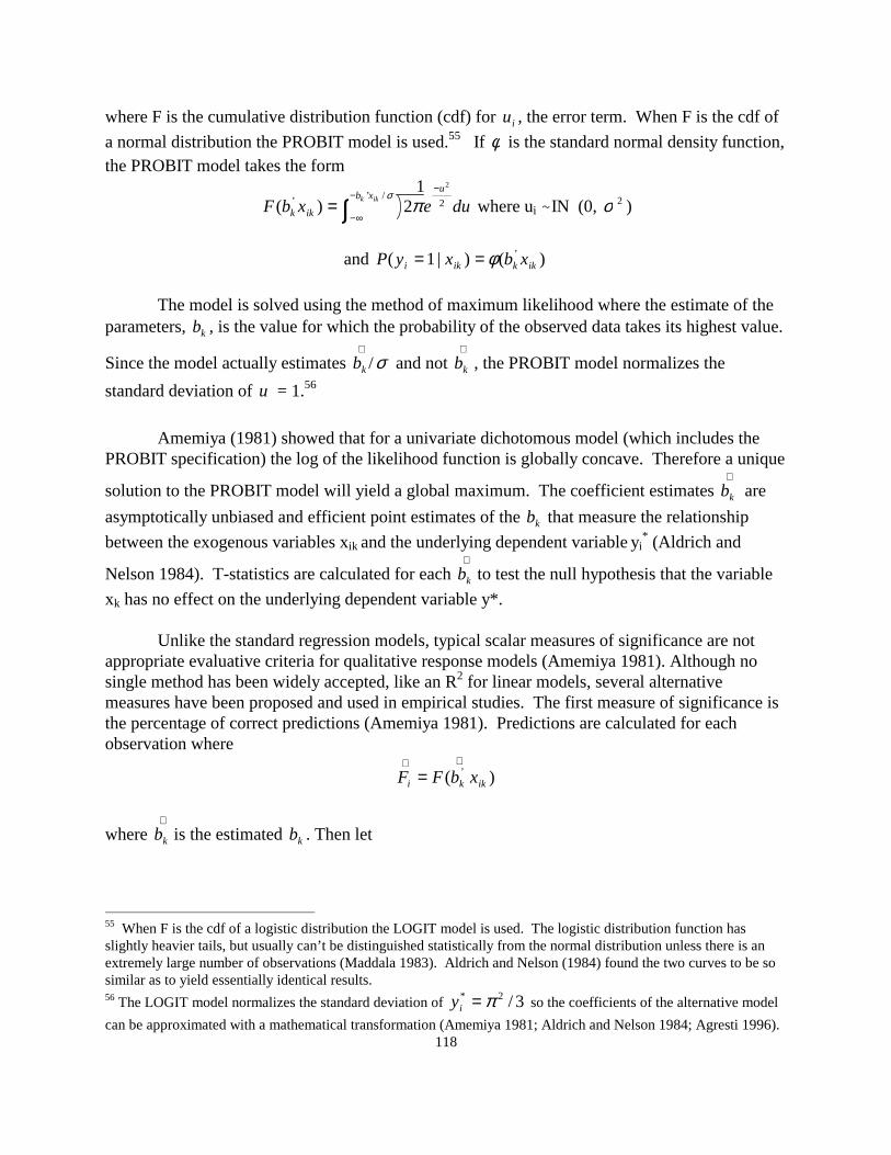
where F is the cumulative distribution function (cdf) for iu , the error term. When F is the cdf of

a normal distribution the PROBIT model is used.55 If φ is the standard normal density function,the PROBIT model takes the form

duexbFu

xb

ikk

ikk 2/’’

212)(

−−

∞−∫= πσ

where ui ~IN (0, 2σ )

and )()|1( ’ikkiki xbxyP φ==

The model is solved using the method of maximum likelihood where the estimate of theparameters, kb , is the value for which the probability of the observed data takes its highest value.

Since the model actually estimates σ/∧

kb and not ∧

kb , the PROBIT model normalizes the

standard deviation of u = 1.56

Amemiya (1981) showed that for a univariate dichotomous model (which includes thePROBIT specification) the log of the likelihood function is globally concave. Therefore a unique

solution to the PROBIT model will yield a global maximum. The coefficient estimates ∧

kb are

asymptotically unbiased and efficient point estimates of the kb that measure the relationship

between the exogenous variables xik and the underlying dependent variable yi* (Aldrich and

Nelson 1984). T-statistics are calculated for each ∧

kb to test the null hypothesis that the variable

xk has no effect on the underlying dependent variable y*.

Unlike the standard regression models, typical scalar measures of significance are notappropriate evaluative criteria for qualitative response models (Amemiya 1981). Although nosingle method has been widely accepted, like an R2 for linear models, several alternativemeasures have been proposed and used in empirical studies. The first measure of significance isthe percentage of correct predictions (Amemiya 1981). Predictions are calculated for eachobservation where

)( ’ikki xbFF

∧∧=

where ∧

kb is the estimated kb . Then let

55 When F is the cdf of a logistic distribution the LOGIT model is used. The logistic distribution function hasslightly heavier tails, but usually can’t be distinguished statistically from the normal distribution unless there is anextremely large number of observations (Maddala 1983). Aldrich and Nelson (1984) found the two curves to be sosimilar as to yield essentially identical results.56 The LOGIT model normalizes the standard deviation of 3/2* π=iy so the coefficients of the alternative model

can be approximated with a mathematical transformation (Amemiya 1981; Aldrich and Nelson 1984; Agresti 1996).

119

2/11 ≥=∧∧

iFifiy

2/10 <=∧∧

iFifiy

The number of incorrect predictions is calculated using the formula

∑=

∧−

N

iii yy

1

2)( .

One disadvantage of this criteria is that if an event happens with a low probability, the number ofcorrect predictions will tend to overestimate the measure of significance (Amemiya 1981).

A second measure of model significance is based on the log-likelihood function (Aldrichand Nelson 1984). The proposed measure is

C = -2 loge )/( 10 ll

Where 1l is the value of the likelihood function for the full model and 0l is the value of the

likelihood function for a restricted model where all the regression coefficients, except for theconstant, are constrained to be zero. The resulting test statistic, C, has a chi-square distribution.

Finally several methods have been proposed to calculate a pseudo-R2. It should be notedthat these statistics can be used only as indicators of significance and not as measures of theproportion of variance in the dependent variable that is explained by the endogenous variables.Two alternative pseudo-R2 measures are shown below.57

0

12 1l

lR −= (McFadden 1974)

)/(2 CNCR += (Aldrich and Nelson 1984)

The variables 1l , 0l , and C are defined as above and N is the number of observations in the

sample.

The estimated coefficients from the PROBIT model cannot be interpreted in the same

way as those from linear regression models. In the PROBIT model ∧

kb measures the effect of a

change in xik on an underlying continuous and unobservable variable yi*. Since the PROBITmodel is non-linear in parameters, the sign of the coefficient estimates determine the direction of

57 Other alternatives for calculating a measure of significance are found in Amemiya (1981) and Maddala (1992).

120

the effect of xk on yi* but the magnitude of the effect depends on ∑=

m

kikk xb

1

’ . The probability that

yi = 1 is not completely determined by ∧

kb (Liao 1994).

The partial derivatives for the probability estimates are used to estimate the marginaleffects of changes in the independent variables on the P(yi = 1). In the PROBIT model

kikkik

ikk

ik

i bxbx

xb

x

yP)(

)()1( ’’

φφ=

∂∂

=∂

=∂

This calculation will provide a close approximation of the marginal effects of a continuousindependent variable on the probability that questionable technical barriers are observed (Liao1994). Often in empirical studies, the marginal effects are calculated at the mean values of xk

since the partial derivatives are functions of the independent variables. T-statistics are calculatedfor each partial derivative to test the null hypothesis that the marginal effect has no significantimpact on the underlying dependent variable y*.

5.3.b. Empirical Results: Aggregate Models

Several specifications of a PROBIT model for the presence or absence of questionabletechnical barriers were estimated using the program LIMDEP (Greene 1991). Observations withmissing data were dropped from the estimation. Previous research has shown that extrapolatingmissing values does not add explanatory power to estimation results (Greene 1997). Theresulting measures of significance, estimated coefficients, and p-values for five alternativemodels are shown in Table 5.5.

121

Table 5.5. Measures of significance, estimated regression coefficients (and p-values)explaining the presence or absence of questionable technical barriers

Model I Model IIModel

IIIModel

IV Model VSample Size:One-observations 44 50 52 52 55Zero-observations: 25 38 38 39 39Measures of Significance:% of correct predictions 86.9 86.4 85.6 86.8 86.2Significance level for chi-

squared statistic.000035 .00001 .0000001 .0000001 .0000001

McFadden R2 .67 .55 .52 .52 .43Aldrich and Nelson R2 .47 .43 .41 .41 .37Independent Variables:*Constant 6.445

(0.105)1.818

(0.208)0.289

(0.775)0.394

(0.645)0.868

(0.012)Individual AgentsKL 0.002

(0.819)-0.002(0.714)

TRDBAL -0.005(0.454)

0.000(0.887)

GTDBAL 0.023(0.756)

USTRD 0.021(0.258)

GUSTRD -0.147(0.082)

-0.034(0.092)

-0.036(0.033)

-0.038(0.027)

-0.030(0.039)

LL 0.846(0.112)

0.581(0.061)

0.617(0.036)

0.610(0.035)

PENTR -0.004(0.129)

-0.002(0.065)

-0.002(0.022)

-0.001(0.004)

-0.001(0.010)

PVT -0.001(0.331)

GFPRCE -0.005(0.166)

Effective Political InfluenceLABAG -0.017

(0.703)-0.049(0.021)

-0.050(0.008)

-0.050(0.008)

RURAL -0.115(0.046)

GDPAG -0.032(0.522)

-0.058(0.058)

-0.051(0.070)

-0.054(0.057)

-0.073(0.000)

122

Table 5.5 (cont.)Effective Political PowerVAAG 0.004

(0.286)-0.001(0.629)

-0.001(0.681)

-0.001(0.654)

GDP 0.001(0.353)

-0.000(0.510)

Policymaker PreferencesGDPEXP -0.002

(0.948)-0.006(0.686)

0.004(0.717)

GOVT -0.192(0.096)

-0.065(0.147)

Institutional StructuresXCHG 0.568

(0.401)TAPPL -0.054

(0.149)-0.020(0.292)

-0.018(0.253)

-0.017(0.274)

-0.020(0.062)

SLACK 0.016(0.204)

0.006(0.461)

0.008(0.342)

0.007(0.346)

TAPPLF -0.016(0.385)

-0.007(0.515)

-0.006(0.580)

-0.005(0.605)

TREDF 0.087(0.173)

0.027(0.293)

0.032(0.145)

0.033(0.140)

WTO 0.441(0.819)

0.709(0.299)

0.955(0.134)

1.012(0.103)

Measurement IssuesFAS 2.300

(0.032)1.555

(0.006)1.808

(0.000)1.827

(0.000)1.709

(0.000)* variable names and definitions can be found in Table 5.1

123

Model I includes all the independent variables identified in the previous section asproxies for the political economy influences on questionable technical barriers. Although ModelI correctly predicts the value of the dependent variable 86.9 percent of the time, there are onlytwo variables, RURAL and FAS, significant at the 5 percent level. Two additional variables,GUSTRD and GOVT, are significant at the 10 percent level, as indicated by the p-values.

Results indicate that the probability of observing questionable technical barriers decreasesas the average change in agricultural trade balance with the U.S. (GUSTRD) increases. Incontrast, the shorter-term measure of bilateral agricultural trade balance with the U.S., USTRD,is not significant in Model I, even at the 10 percent level. The probability of questionabletechnical barriers decreases as the proportion of rural population (RURAL) increases. Resultsalso indicate that as the percentage of government spending (GOVT) increases the probability ofobserving questionable technical barriers decreases. The presence of an FAS post (FAS)increases the probability that barriers will be observed.

There are only 69 observations included in Model I due to limitations in the availability inone or more of the independent variables. The sample includes 44 countries that apply one ormore questionable technical barriers and 25 countries that do not apply such barriers. As shownin Table 5.2, observations are most limited for the variables GTDBAL, GFPRCE, and XCHG,none of which are significant at the 10 percent level in Model I.

In addition, as shown in Table 5.3, there is a high degree of correlation between theindependent variables RURAL and LABAG (0.830), and PVT and GDP (0.992) included inModel I. Several authors have recently argued that high correlation coefficients betweenexplanatory variables are not sufficient criteria to identify multicollinearity (Maddala 1992;Spanos and McGuirk 1998). Nevertheless, the high correlation between PVT and GDP doesindicate that PVT is reflecting national income levels. The high correlation between RURALand LABAG may indicate that RURAL is not picking up the broader secondary effects of policydecisions on rural communities when compared to LABAG.

In Model II the variables GTDBAL, PVT, GFPRCE, RURAL, XCHG, and USTRD aredropped from the regression. Results indicate that there are only small changes in somemeasures of significance between Model I and Model II. There is a 0.5 decrease in thepercentage of correct predictions. The McFadden and Aldrich and Nelson pseudo-R2 measuresfall to .55 and .43, respectively, but the overall significance of Model II increases compared toModel I, as measured by the chi-squared statistic. The variable LABAG becomes significant atthe 5 percent level and the variables PENTR, LL and GDPAG become significant at the 10percent level, as measured by the p-values. The variables GUSTRD and FAS remain statisticallysignificant in Model II but GOVT becomes insignificant, even at the 10 percent level.

Consistent with Model I results, as the average change in agricultural trade balance withthe U.S. (GUSTRD) increases the probability of questionable technical barriers decrease. Inaddition, the probability of enacting questionable technical barriers increases as the number ofagricultural workers increases relative to the amount of productive land available (LL), but

124

decreases as the proportion of labor employed in agriculture increases relative to the size of thepopulation (LABAG). Results of Model II indicate that the probability of countries enactingquestionable technical barriers decreases as imports increase relative to the size of the domesticagricultural sector (PENTR). As a measure of effective political power, when the relativecontribution of agriculture to GDP (GDPAG) increases the probability of enacting questionabletechnical barriers decreases. The presence of an FAS post (FAS) increases the probability thatbarriers will be observed.

The independent variables KL, TRDBAL, and GDP change sign in Model II compared toModel I, indicating that these estimated parameters may not be stable. All three of thesevariables remain statistically insignificant, even at the ten percent level.

In Model III the variables KL, TRDBAL, GDP, and GOVT are dropped from thespecification. The percentage of correct predictions decreases by 0.8 to 85.6 percent withcorresponding small drops in the pseudo-R2 measures to .52 and .41, respectively. Thesignificance level of LABAG increases to the 1 percent level and the significance levels ofPENTR, LL, and GUSTRD increase to the 5 percent level. In addition, the number ofobservations included in the sample increases by two to 90. There is a sign change on thevariable GDPEXP.

Consistent with Models I and II, results indicate that the probability of questionabletechnical barriers increases with increased geographic concentration of agricultural workers (LL)and the presence of an FAS post (FAS). The probability of questionable technical barriersdecreases with increased growth in agricultural trade balance with the U.S. (GUSTRD), withincreased penetration of imports relative to domestic production (PENTR), with an increasedproportion of agricultural workers (LABAG), and with an increased percentage contribution ofagriculture to GDP (GDPAG).

In Model IV the variable GDPEXP is dropped from the specification due to the parameterinstability demonstrated in the previous models. The number of correct predictions increasesfrom 85.6 percent in Model III to 86.8 percent in Model IV. The overall significance of themodel does not change, as measured by the chi-square statistic and the pseudo-R2 measures donot change. The variables WTO becomes almost significant at the 10 percent level, as measuredby the p-values.

Again, results indicate that the probability of questionable technical barriers increaseswith increased geographic concentration of agricultural workers (LL) and the presence of an FASpost (FAS). The probability of questionable technical barriers decreases with increased growthin agricultural trade balance with the U.S. (GUSTRD), with increased penetration of importsrelative to domestic production (PENTR), with an increased proportion of agricultural workers(AGLAB), and with an increased percentage contribution of agriculture to GDP (GDPAG). Inaddition, results of Model IV indicate that the probability of questionable technical barriersincreases for WTO members. Although in Model IV, the variable WTO is almost significant at

125

the 10 percent level, none of the other measures of institutional structure (TAPPL, SLACK,TAPPLF, and TREDF) are statistically significant, consistent with the results of Models I-III.

Model V is a more parsimonious specification of the model explaining the presence orabsence of questionable technical barriers.58 All of the independent variables included in ModelV are significant at the 5 percent level or better except for TAPPL which is significant at the 10percent level. In addition, Model V is based on an increased number of observations comparedto the previously reported models. In Model V, 55 countries applied one or more questionabletechnical barriers and 39 countries did not apply such barriers. Model V correctly predicts theoutcome 86.2 percent of the time and has gained in overall significance compared to Model I,where all the original independent variables were included, as measured by the chi-squarestatistic. There is however a decrease in the pseudo-R2 between Model I and Model V. TheMcFadden R2 drops from .67 to .43 and the Aldrich and Nelson R2 drops from .47 to .37 betweenthe two specifications. The estimated coefficients in Model V were all within a 95 percentconfidence interval constructed for the same variables in Model I, indicating that the estimatedparameters are stable across specifications.

Consistent with the results of Models I-IV, results from Model V indicate that theprobability of questionable technical barriers decreases with increased growth in agriculturaltrade balance with the U.S. (GUSTRD), with increased penetration of imports relative todomestic production (PENTR), and with an increased percentage contribution of agriculture tonational income (GDPAG). Results from Model V indicate that the probability of questionabletechnical barriers decreases as the projected 1999 tariff on agricultural products (TAPPL)increases. The probability of questionable technical barriers increases with the presence of anFAS post (FAS).

In order to use a model for statistical inference it must be correctly specified. Since theunit of analysis in these specifications is countries, it is possible that the variance is not constant.Therefore Model V was tested for heteroskedasticity using the log-likelihood test described inGreene (1991). The null hypothesis that homoskedasiticity was the correct assumption could notbe rejected at the 1 percent significance level.

Despite the increased number of observations included in Model V compared to ModelsI-IV, the sample is still smaller than the initial set of observations. A list of countries deletedfrom the original sample in order to estimate Model V is included in Appendix D. Table 5.6shows the summary statistics for the observations used to estimate Model V. The values in Table5.6 can be compared to similar statistics for the entire set of observations, as shown earlier inTable 5.2, to indicate any possible sub-sample bias.59 Questionable technical barriers are presentin 58 percent of the countries in the sample compared to 47 percent of the countries in the entire 58 Many specifications of more parsimonious models were estimated starting with the variables included in Model IVand following the general procedures outlined in Leamer (1978) for simplification and proxy variable searches formodel selection. In addition, the model reported minimizes Akaike’s information criteria (Akaike 1977) which isproposed in Maddala (1992) as a statistical criteria for selection of regressors in non-linear models when theoreticaldeterminations cannot be made.59 A table of correlation coefficients for the variables and observations included in Model V is shown in Appendix E.

126

data set. The mean of GUSTRD is higher in the sample, 1.08 percent compared to –2.84 percentwhen all the observations are included as some of the lowest observations for GUSTRD havebeen deleted. The mean value of FAS is also increased in the sample. Now 48 percent of theobservations have an FAS post compared to 38 percent in the entire data set. The summarystatistics for PENTR, GDPAG, and TAPPL are not very different between the Model V sub-sample and the entire set of observations. The entire range of values for these three variables isincluded in the sample as the maximum and minimum values remain the same.

Table 5.6. Summary statistics for variable observations included in Model V

Variable* MeanStandardDeviation Median Maximum Minimum

YN 0.58 0.49 1.00 1.00 0.00GUSTRD 1.08 40.58 -0.07 333.70 -175.40PENTR 153.73 644.12 30.84 5108.60 2.66GDPAG 16.36 14.49 12.00 67.00 0.00TAPPL 8.58 16.99 1.10 65.10 -21.40FAS 0.48 0.50 0.00 1.00 0.00* variable names and definitions can be found in Table 5.1

5.3.c. Discussion of Aggregate Model Results

Although the coefficients of the PROBIT model cannot be used directly to measure themarginal effects of the independent variables, they do indicate the direction and the relativemagnitude of the effects. The percentage change in agricultural trade balance with the U.S.(GUSTRD) is negatively related to the probability of enacting questionable technical barriers.As the change in the agricultural trade balance becomes more favorable, exports to the U.S.increase relative to imports from the U.S. and the probability of supplying economic-basedprotection through technical barriers decreases. This supports the hypothesis that protection willdecrease when export competition is lessened and producers perceive having less to gain fromregulatory intervention. In contrast to the average change in such a balance, the per capitabilateral agricultural trade balance with the U.S. in the previous year (USTRD) was notsignificant in the empirical models. It may be that producers only recognize and react to longer-term trends in trade balance. Or it could be that the cross-sectional nature of the dependentvariable is masking any short-term policy response; it may take longer than one year forregulatory intervention to be achieved.

In addition, the statistical relationships of the percentage change in agricultural tradebalance with the U.S. to total agricultural trade balance and to the change in total trade balance issmall, as evidenced by correlation coefficients of 0.018 and –0.009, respectively. ThereforeGUSTRD is not just reflective of the overall agricultural trade balance or its growth. Thenegative coefficient on GUSTRD in particular provides some evidence in support of thehypothesis that countries follow a retaliatory or tit-for-tat regulatory strategy, although such a

127

hypothesis cannot be measured directly without information on U.S. technical barriers. In a tit-for-tat strategy, policymakers increase technical barriers on products from a particular country inretaliation for an increase of such trade barriers applied to their own exports and the resultingdecrease in the bilateral trade balance. Even when the overall agricultural trade balance(TRDBAL) is held constant, a worsening in the agricultural trade balance with the U.S. increasesthe probability of enacting questionable technical barriers.

Neither the capital-land ratio, nor two of the variables included as proxies for theeconomic stakes of individual agents as consumers (PVT and GFRPCE) are identified assignificant determinants of the presence or absence of questionable technical barriers. This maysupport the hypothesis that producers, who are less numerous, have higher individual economicstakes in regulatory intervention, and are better able to organize and influence the policyoutcomes in their favor. In contrast, consumers who are more numerous, may have lowerindividual stakes and be less able to organize.

However, as another measure of the preferences of individual agents, when the import ofagricultural products increases relative to domestic production levels (PENTR), the probability ofenacting questionable technical barriers decreases. The penetration ratio will be larger incountries with relatively small domestic agricultural production sectors compared to nationalconsumption, for example Hong Kong. In these cases, the empirical results support thehypothesis that consumers have more to lose if the difference between the domestic and worldprice increases as a result of regulatory intervention and implies that they are able to dominatethe effect of producer gains from regulatory intervention when import competition is greater.The penetration ratio will be smaller in countries where imports are small relative to value-addedin agriculture, for example New Zealand. In these cases, the empirical results support thehypothesis that producers perceive having more to gain from intervention and implies that theyare able to dominate the effect of any potential consumer gains when there is less importcompetition. Even though statistical simultaneity is avoided by measuring the level ofagricultural import penetration in the previous year, without a time lag imports could bemeasured as a function of trade restrictiveness. However, as a government typically enacts manytypes of trade barriers, it seems more likely that decisions on the use of questionable technicalbarriers are taken in reaction to the aggregate conditions of agricultural import penetration. Inaddition, technical barriers are regulatory policies applied to specific commodities and the impactrelative to total agricultural imports is small.

Results indicate that the agricultural labor-land ratio (LL) serves as one proxy foreffective political influence of agricultural interests. A positive sign supports the hypothesis thatas the number of workers becomes more geographically concentrated, the probability of enactingquestionable technical barriers increases. This effect appears to dominate the use of the labor-land ratio as a proxy for the potential economic stakes to agricultural workers as the stakes wouldrise as the labor-land ratio decreased and there are fewer workers to share any potential gains ineconomic rents.

128

The percentage of the labor force employed in agriculture (LABAG) is another proxy foreffective political influence. A negative coefficient supports the Olson hypothesis that as thepercentage labor force in agriculture increases, the ability of the group to organize, overcomefree-rider problems, and lobby successfully for protection decreases. Even when the geographicconcentration of agricultural workers (LL) is held constant, an increase in the percentage of thepopulation employed in the sector results in a decrease in the probability of economic-basedprotection through questionable technical barriers.

The percentage contribution of agriculture to GDP (GDPAG) is included as anothermeasure of effective political power. When the relative contribution of agriculture to GDPincreases the probability of enacting questionable technical barriers decreases. In contrast, theabsolute contribution of agriculture to the economy (VAAG) is not shown to have a statisticallysignificant effect on the probability of enacting questionable technical barriers. The negativesign on GDPAG provides further support for the Olson hypothesis. As the agricultural sector is alarger proportion of the economy, it may be harder for producers to organize and effectivelyinfluence policy outcomes resulting in a lower probability of enacting questionable technicalbarriers. Model V was re-estimated holding income constant by including the GDP variablefrom Model I. Results indicate that the percentage contribution of agriculture still had astatistically significant negative impact on the probability of observing questionable technicalbarriers.

Suprisingly, in this dataset, the variables for per capita income (GDP and PVT) were notsignificant determinants of the presence or absence of questionable technical barriers. Althoughthe correlation between GDPAG and GDP in the data set is only –0.531, the negative sign isconsistent with the hypothesis that policymakers are more likely to tax (disprotect) agriculturewhen the relative contribution of the sector is higher. Although there is no direct evidence tosupport the income hypothesis through the GDP variable, the result for GDPAG suggests thattechnical barriers are relatively less likely to be observed in developing countries with a higheragricultural to nonagricultural GDP ratio.

The proxies for policymaker preferences are not shown to be significant determinantsexplaining the presence or absence of questionable technical barriers. In Models I-III, theestimated parameter on the percentage of exports in GDP (GDPEXP) was not stable, as indicatedby changing signs, or statistically significant. The percentage of government consumption inGDP (GOVT) was marginally significant in Model I but became insignificant in subsequentspecifications. It is likely that these proxies for outward- and inward-looking market orientationare not precise enough measures to separate policymaker preferences from the other politicaleconomy factors. Direct measures of support, such as contributions or other lobbying activities,might prove to be more accurate proxies but are not readily available on as wide a cross-countrybasis as needed for these models.

As a measure of institutional structures, the projected 1999 most-favored-nation averageapplied tariff rate on agricultural products, including the tariffication of non-tariff barriers,(TAPPL), is negatively related to the probability of enacting questionable technical barriers. This

129

result provides evidence to support the hypothesis that technical barriers may be used assubstitutes for tariffs and other non-tariff barriers lowered through GATT obligations. None ofthe other variables included to represent institutional structure, SLACK, TAPPLF, or TREDF,were statistically significant in any of the models measuring the presence or absence ofquestionable technical barriers and TAPPL was only a significant measure of institutionalstructures when these other variables were dropped from the specification. Model V wasreestimated holding WTO membership constant by including the variable WTO in thespecification. Results indicate that the probability of questionable technical barriers is higherwhen future tariff rates are lower (the p-value on TAPPL is 0.063), even when countries havecommitted to the SPS and TBT Agreements and face the possibility of international challenge inthe WTO (the p-value on WTO is 0.688).

Results indicate that countries that are members of the WTO are more likely to enactquestionable technical barriers despite commitments to the GATT Agreements including the SPSand TBT Agreements and the Agreement on Agriculture. It may be that the provisions of theSPS and TBT Agreement have not fully constrained the misuse of technical barriers. A positivecoefficient on WTO is consistent with the negative coefficient on the future applied tariff rate(TAPPL) and provides support for the hypothesis that countries that are constrained in the use ofother trade measures may increase the use of questionable technical barriers, WTO Agreementsnotwithstanding.

The dummy variable included to measure the possible impact of the survey design, FAS,is also statistically significant and positively related to the probability of observing questionabletechnical barriers. Questionable technical barriers are more likely to be reported in countrieswhere an FAS post is present, indicating that such trade restrictions are either over-reported incountries where an FAS post is present or under-reported in countries without an FAS post.60

Although there is no direct evidence for which direction of reporting is correct, of the 63countries where questionable technical barriers were present, 45 had more than one barrierreported, indicating an increased likelihood that at least one questionable measure was in place.

5.3.d. Empirical Results: Marginal Effects

Due to the non-linearity of the PROBIT models, the estimated coefficients cannot bedirectly interpreted as constant marginal effects of the independent variables, as they are in thelinear models. In the PROBIT models, marginal effects are point estimates and must becalculated at specified values of the independent variables. The marginal effects of the changesin the continuous independent variables for Model V are calculated when the independentvariables are set equal to their mean values. Results and the associated p-values are shown inTable 5.7.

60 Model V was respecified to include FAS as a slope shifter, as well as a mean shifter. In these models, FAS did nothave a statistically significant impact on the slope of the regression function.

130

Table 5.7. Marginal effects from changes around the mean of the independent variablesused in Model V on the probability of observing questionable technical barriers

Independent Variable* Marginal Effect P-valueGUSTRD -0.012 0.043PENTR -0.0003 0.011GDPAG -0.028 0.004TAPPL -0.008 0.061* variable names and definitions can be found in Table 5.1

At the mean, a 1 percent increase in GUSTRD would decrease the probability by 1.2percent, ceteris paribus and a 1 percent increase in PENTR would decrease the probability ofobserving questionable technical barriers by 0.03 percent, ceteris paribus. The marginal effect ofGDPAG is larger at the mean and statistically significant at the one percent level as measured bythe p-value. A 1 percent increase in the percentage contribution of agriculture to GDP woulddecrease the probability of observing questionable technical barriers by 2.8 percent. A 1 percentincrease in TAPPL would decrease the probability by 0.8 percent.

For comparison, the levels of three independent variables, GUSTRD, GDPAG, andTAPPL were adjusted sequentially to provide a series of marginal effect observations over therange of their values. Values of GUSTRD vary from –244 to 334 over the entire range ofobservations in the data set (see Table 5.2). The marginal effects of changes in GUSTRD weresignificant between the values of –25 and 50, the values shown in Figure 5.1. The highestmarginal impact from changes in GUSTRD is observed when the change in agricultural tradebalance with the U.S. was approximately 5 percent. At this value of GUSTRD the marginaleffect on P(Y=1) is almost 1.2 percent. 61 The lowest marginal impact from a change inGUSTRD is observed when the value was large. A small change in GUSTRD around 50 resultsin a 0.54 percent change in the P(Y=1). The marginal effect also decreases when the values ofGUSTRD are negative. At a small change from a negative 25 percent average change in tradebalance with the U.S., the probability of observing questionable technical barriers decreases by0.74 percent.

61 The probability of observing questionable technical barriers is represented in the statistical models by theprobability of a positive response in the latent dependent variables, or by the P(Y=1) in the PROBIT specifications.

131

0

0.002

0.004

0.006

0.008

0.01

0.012

0.014

-25 -15 -5 0 5 15 25 50

Values of GUSTRD

Mar

gin

al e

ffec

t o

n P

(Y=1

)

Figure 5.1. Marginal Effect of GUSTRD on the Probability of Observing QuestionableTechnical Barriers

The contribution of agriculture to GDP ranges from zero to 67 percent across the entiredata set (see Table 5.2). When the marginal effects are calculated over this range they aresignificant between zero and 40 percent, the range shown in Figure 5.2. The impact of GDPAGis highest when agriculture contributed approximately 20 percent to the national economy. Atthis level, a small change in GDPAG decreases the probability of observing questionabletechnical barriers by approximately 3 percent. The marginal impact of GDPAG decreases at bothlower and higher levels of agricultural contribution. When GDPAG is zero, a small changedecreases the P(Y=1) by approximately one percent. When GDPAG is 40 percent, a smallchange decreases the P(Y=1) by slightly less than one percent.

132

0

0.005

0.01

0.015

0.02

0.025

0.03

0.035

0 5 10 15 20 25 35 40

Values of GDPAG

Mar

gin

al e

ffec

t o

n P

(Y=1

)

Figure 5.2. Marginal Effect of GDPAG on the Probability of Observing QuestionableTechnical Barriers

Values of TAPPL range from –21.40 to 65.10 in the entire data set (see Table 5.2). Themarginal effect of changes in TAPPL are significant between the values of –20 and 50, the rangeof values shown in Figure 5.3. The largest impact on P(Y=1) from a change is observed whenthe value of TAPPL is between 10 and 25 percent. The marginal effect of a one percent increasein the average tariff on agricultural products when the tariff is approximately 15 percent is a 0.79percent decrease in the probability of observing questionable technical barriers, ceteris paribus.The lowest impact on P(Y=1) from a change is observed when the applied tariff rate is negativeindicating that export subsidies are applied. A one percent increase in the average tariff when thetariff is approximately –20 percent decreases the probability of observing questionable technicalbarriers by 0.57 percent, ceteris paribus.

133

0

0.001

0.002

0.003

0.004

0.005

0.006

0.007

0.008

0.009

-20 -15 -10 -5 0 5 10 15 25 50

Values of TAPPL

MA

rgin

al e

ffec

t o

n P

(Y=1

)

Figure 5.3. Marginal Effect of TAPPL on the Probability of Observing QuestionableTechnical Barriers

Since marginal effects vary over the range of the independent variables, a series of staticcomparisons are made for changes in the probability of enacting questionable technical barriers.The value of each continuous independent variable is increased systematically by one standarddeviation above its mean with the other variables set equal to their mean values. As shown inTable 5.8, when GUSTRD increases from 1.08 to 41.66 percent, the P(Y=1) decreases by 42.2percentage points. When the percentage of agricultural imports relative to domestic production(PENTR) increases from 153.73 to 797.85 the P(Y=1) decreases by 16.4 percentage points. Asthe applied tariff rate (TAPPL) increases from 8.58 to 25.57 percent, the P(Y=1) decreases by13.5 percentage points. Probabilities associated with changes in percentage contribution toagriculture (GDPAG) are similar in magnitude to those of GUSTRD. As the percentagecontribution of agriculture to GDP (GDPAG) increases from 16.36 to 30.85 percent, P(Y=1)decreases by 38.1 percentage points.

134

Table 5.8. Effects of static changes in independent variables on the probability of observingquestionable technical barriers

Value of the Independent Variable* Probability that Y=1

GUSTRD = 41.66 .155GUSTRD = 1.08 .577

PENTR = 797.85 .413PENTR = 153.73 .577

GDPAG = 30.85 .196GDPAG = 16.36 .577

TAPPL = 25.57 .442TAPPL = 8.58 .577* the lower value represents the mean and the upper value represents the mean plus one standard

deviation, with the value of the other independent variables set equal to their mean

Interpretation of the effect of a change in FAS is similar. While it is the presence of anFAS post raises the probability of questionable technical barriers being reported, interpretation ofa marginal effect is meaningless since the value of FAS is restricted, by definition, to zero or one.A better estimate of the impact of a change on the probability is the difference between predictedprobability conditional on the two categories of FAS, as shown in Table 5.9. At the mean of theother independent variables, the probability of observing questionable technical barriers to U.S.agricultural trade increases by 43.1 percent when a FAS post is located in that country, ceterisparibus.

Table 5.9. Effects of a FAS post on the probability of observing questionable technicalbarriers

Value of FAS Probability that Y=1FAS = 0 .267FAS = 1 .698

5.3.e. Empirical Results: Desegregated Models

In order to provide additional insights on the effect of the explanatory variables, Model Vis modified to include additional information about the characteristics of questionable technicalbarriers as described in Chapter Four. There are two possible ways to include this information inthe empirical specifications. The first is by including a series of dummy variables. Thisapproach will estimate the impact of legal classification, regulatory goal, market impact, policyinstrument, and product group on the intercept and/or slope of the PROBIT function. The second

135

method is to modify the dependent variable to reflect the presence or absence of questionabletechnical barriers in the specified category and rerun the original model. This approach willmeasure the relative influence of the independent variables in explaining the presence or absenceof technical barriers in each of these categories. The second method was used in this study tobuild evidence supporting the robustness of the independent variables as determinants of theincidence of questionable technical barriers.

5.3.e.1. Legal Classification

Over 85 percent of the technical barriers identified by the USDA survey were governedby the SPS Agreement and, in the sample used for model estimation, only one country thatapplied questionable technical barriers did not apply questionable SPS barriers. Therefore therewere not many substantial changes in the results from Model V when the dependent variable wasmeasured as the presence of questionable SPS barriers (see Table 5.10). All the estimatedcoefficients retain the same signs. The variable GUSTRD becomes less significant. Converselythe significance level of the coefficient on the applied tariff rate (TAPPL) increases. Thecoefficient on FAS decreases but is still relatively large when compared to the coefficients for theother independent variables, indicating that the relative magnitude of the impact from thisvariable may be larger.

136

Table 5.10. Measures of significance, estimated regression coefficients (and p-values)explaining the presence or absence of questionable technical barriers by legalclassification

Dependent VariablePresence of

technical barriers(Model V)

Presence ofSPS barriers

Presence ofother technical

barriersSample Size:One-observations 55 54 15Zero-observations 39 40 79Measures of Significance:% of correct predictions 86.2 83.0 84.0Significance level for chi-squarestatistic

.0000001 .0000000004 .0008

McFadden R2 .43 .39 .26Aldrich and Nelson R2 .37 .35 .18Independent Variables:*Constant 0.868

(0.012)0.761

(0.021)1.483

(0.004)GUSTRD -0.030

(0.039)-0.027(0.056)

0.002(0.722)

PENTR -0.0006(0.010)

-0.0006(0.015)

-0.00004(0.842)

GDPAG -0.073(0.0002)

-0.064(0.0003)

-0.042(0.075)

TAPPL -0.020(0.062)

-0.021(0.044)

-0.003(0.801)

FAS 1.709(0.00004)

1.545(0.00007)

1.472(0.003)

* variable names and definitions can be found in Table 5.1

When the dependent variable was measured as the presence of questionable technicalbarriers governed by either the TBT Agreement, multiple Agreements, or other provisions ofGATT 1994 there were only 15 positive observations. As measured by the chi-square statistic,the model does not explain very well. Only FAS remains significant at the 1 percent level andGDPAG remains significant at the 10 percent level. There is a sign change on the coefficient forGUSTRD. The percentage of correct predictions remains high (84.0), providing empiricalevidence that this measure will be overestimated in cases where the P(Y=1) is low. The othermeasures of significance are much lower for this model. The McFadden and Aldrich and Nelsonpseudo-R2’s are .26 and .18 respectively.

137

5.3.e.2. Regulatory Goal

The entire sample of observations was disaggregated according to regulatory goals.Models were run to estimate the effect of the Model V independent variables on the presence orabsence of questionable technical barriers that were justified as measures to protect commercialanimal and plant health, ensure food safety, and ensure product quality. Results from the threemodels are shown in Table 5.11.

The econometric model explains 68.1 percent of the outcomes when questionabletechnical barriers are enacted with the stated regulatory goal of protecting commercial animal andplant health. The independent variables GDPAG and FAS remain statistically significant at theone percent level. As agriculture contributes a larger share to national GDP, policymakers aremore likely to enact questionable technical barriers with the goal of preventing pest and diseaseinfestations in commercial production.

As measured by the chi-squared statistic or the pseudo R2’s the econometric model doesnot explain the presence of questionable technical barriers as well when the stated goal is foodsafety. The variable GDPAG remains significant at the one percent level providing someevidence to contradict the hypothesis that food safety concerns, at least as a stated regulatory goalfor questionable policies, are more prevalent among wealthier economies.

138

Table 5.11. Measures of significance, estimated regression coefficients (and p-values)explaining the presence or absence of questionable technical barriers byregulatory goal

Dependent VariablePresence of barriers

for commercialproduction

Presence ofbarriers forfood safety

Presence ofbarriers for

product qualitySample Size:One-observations 41 34 12Zero-observations 53 60 82Measures of Significance:% of correct predictions 68.1 70.2 87.2Significance level for chi-

square statistic.0000039 .000953 .04046

McFadden R2 .26 .17 .16Aldrich and Nelson R2 .26 .18 .11Independent Variables:*Constant 0.568

(0.161)0.068

(0.831)-1.326(0.003)

GUSTRD -0.012(0.351)

-0.001(0.904)

0.001(0.857)

PENTR -0.003(0.113)

-0.000(0.275)

0.000(0.871)

GDPAG -0.057(0.001)

-0.479(0.003)

-0.034(0.124)

TAPPL -0.003(0.710)

-0.004(0.643)

0.007(0.458)

FAS 0.717(0.025)

0.588(0.050)

0.807(0.054)

* variable names and definitions can be found in Table 5.1

There were only 12 positive observations when product quality was the stated goal forquestionable technical barriers. The econometric model did not explain the presence of thesebarriers well as measured by either the chi-squared statistic or the R2. The percentage of correctpredictions was high, 87.2 percent, but a closer examination of individual predictions indicatesthat no positive outcomes were predicted. Therefore, in this case, 87.2 simply represents theproportion of zero observations in the sample.

5.3.e.3. Market Restriction

Model V was modified and rerun to reflect the presence of questionable market access,expansion and retention barriers as described in Chapter Four. Results are shown in Table 5.12.

139

Table 5.12. Measures of significance, estimated regression coefficients (and p-values)explaining the presence of questionable technical barriers by market restriction

Dependent VariablePresence of

access barriersPresence of

expansion barriersPresence of

retention barriersSample Size:One-observations 29 41 17Zero-observations 65 53 77Measures of Significance:% of correct predictions 72.3 78.7 80.9Significance level for chi-square

statistic.00003 .00000001 .0078

McFadden R2 .24 .35 .18Aldrich and Nelson R2 .23 .32 .14Independent Variables:*Constant 0.997

(0.066)0.037

(0.914)-1.013(0.010)

GUSTRD 0.002(0.686)

-0.015(0.318)

0.001(0.791)

PENTR -0.008(0.058)

-0.0009(0.201)

-0.00006(0.781)

GDPAG -0.088(0.001)

-0.047(0.006)

-0.029(0.139)

TAPPL -0.004(0.667)

-0.011(0.235)

-0.016(0.102)

FAS -0.283(0.396)

1.494(0.00001)

1.014(0.006)

* variable names and definitions can be found in Table 5.1

The models for access and retention barriers are relatively insignificant as measured bythe chi-square statistic or the pseudo-R2 measurements. Both include only one variable which issignificant at the 1 percent level. However the model for retention barriers has a higherpercentage of correct predictions than the other two models.

The model for expansion barriers predicts 78.7 percent of the outcomes correctly. It ishighly significant as measured by the chi-squared statistic and has McFadden and Aldrich andNelson R2’s equal to .35 and .32 respectively. The variables GDPAG and FAS remainsignificant at the 1 percent level. Both of the significant variables retain the same signs as ModelV. The coefficient on FAS is large relative to the other independent variables indicating arelatively larger magnitude of impact on the probability of observing questionable expansionbarriers.

140

5.3.e.4. Policy Instrument

The observations in the sample were categorized by the presence or absence ofquestionable technical barriers enacted through bans, process standards, or product standards.Model V was rerun to assess the effect of previously identified determinants on barriers by thesepolicy instruments. Measures of significance, estimated coefficients, and p-values for these threemodels are shown in Table 5.13.

Table 5.13. Measures of significance, estimated regression coefficients (and p-values)explaining the presence or absence of questionable technical barriers by policyinstrument

Dependent VariablePresence of

bansPresence of

process standardsPresence of

product standardsSample Size:One-observations 18 37 23Zero-observations 76 57 71Measures of Significance:% of correct predictions 80.8 73.4 76.6Significance level for chi-square

statistic.07000 .0000008 .003299

McFadden R2 .11 .29 .17Aldrich and Nelson R2 .10 .28 .16Independent Variables:*Constant 0.068

(0.901)0.205

(0.534)-0.069(0.895)

GUSTRD -0.001(0.799)

-0.017(0.332)

0.001(0.835)

PENTR -0.009(0.123)

-0.000(0.139)

-0.007(0.136)

GDPAG -0.037(0.054)

-0.069(0.000)

-0.042(0.038)

TAPPL -0.009(0.355)

-0.003(0.771)

-0.006(0.514)

FAS 0.171(0.629)

0.939(0.004)

0.681(0.047)

* variable names and definitions can be found in Table 5.1

Although there were 66 barriers identified in the 1996 USDA Survey that were enacted asproduct bans, only 18 countries applied such policies in the econometric specifications. As aresult, the econometric model does not do a good job in explaining the presence or absence ofquestionable product bans. The independent variable GDPAG is the only variable statisticallysignificant at the 10 percent level or better.

141

There are 37 countries identified as applying questionable technical barriers whereprocess standards are the policy instrument. Both GDPAG and FAS are statistically significantvariables at the one percent level. The model explains well as measured by the chi-squaredstatistic. The same two independent variables remain significant when product standards are thepolicy instrument used in questionable technical barriers. However, as measured by the chi-squared statistic or the psdudo-R2 measures, the model does not do as good a job in explainingthe presence of these barriers.

5.3.e.5. Product Category

Model V was again modified to reflect the product category affected by questionabletechnical barriers. Product categories were described in Chapter Four and include animal, grain,fruit/vegetable, and processed products, as shown in Table 5.14. Only the models for animal andprocessed products include any variables which are significant at the one percent level and themodel for fruit/vegetable products does not include any significant variables even at the 10percent level.

As measured by the chi-squared statistic, the model does not explain the probability of abarrier as well for the models of grain, fruit/vegetables, and processed products compared to themodel for animal products. In the animal products model the variables GUSTRD and TAPPLremain significant at the 10 percent level and the variables GDPAG and FAS remain significantat the 1 percent level. There are no significant variables at the 10 percent level in the model forfruit/vegetable products. Still the McFadden and Aldrich and Nelson R2 in the fruit/vegetablemodel are .34 and .24 respectively. The percentage of correct predictions and McFadden R2 arehigher for the fruit/vegetable model than any of the other three models for product groups,indicating that while this model does not explain the presence of barriers to fruit/vegetableproducts very well (no significant variables) it can predict the presence of such barriers. Onlyseven of the 17 countries which apply questionable technical barriers to fruit and vegetableproducts are among the 18 countries which apply such barriers to processed products.

142

Table 5.14. Measures of significance, estimated regression coefficients (and p-values)explaining the presence or absence of questionable technical barriers byproduct category

Dependent VariablePresence

of barriersto animalproducts

Presenceof barriers

to grainproducts

Presence ofbarriers to

fruit/vegetableproducts

Presence ofbarriers toprocessedproducts

Sample Size:One-observations 40 22 17 18Zero-observations 54 72 77 76Measures of Significance:% of correct predictions 67.0 78.7 82.9 81.9Significance level for chi-

square statistic.000004 .0159 .00001 .0017

McFadden R2 .26 .14 .34 .21Aldrich and Nelson R2 .25 .12 .24 .17Independent Variables:*Constant 0.353

(0.270)-0.496(0.219)

-5.339(0.911)

-0.833(0.049)

GUSTRD -0.026(0.096)

0.0008(0.863)

0.004(0.605)

0.002(0.752)

PENTR -0.0004(0.103)

-0.0009(0.535)

-0.00004(0.852)

-0.0008(0.513)

GDPAG -0.058(0.001)

-0.033(0.060)

-0.006(0.769)

-0.046(0.037)

TAPPL -0.017(0.059)

-0.006(0.482)

-0.009(0.354)

-0.001(0.904)

FAS 0.872(0.006)

0.668(0.046)

5.230(0.913)

1.005(0.009)

* variable names and definitions can be found in Table 5.1

5.3.f. Summary

Modeling the presence or absence of questionable technical barriers in a PROBITframework begins to identify the determinants of the incidence of such barriers. The percentagechange in agricultural trade balance with the U.S. is negatively related to the probability ofenacting questionable technical barriers. As the agricultural trade balance with the U.S.improves by one percent (exports increase relative to imports) the probability of enactingquestionable technical barriers decreases by 1.2 percent at the mean of the data, ceteris paribus.

143

A one standard deviation improvement in the trade balance decreases the probability by over 42percent. When the trade balance with the U.S. had either decreased or increased by largeamounts in the last three years, a small additional change had less effect on the probability ofenacting questionable technical barriers. This suggests that when the agricultural tradingrelationship has changed by a large amount, policymakers are less likely to react to small changesby providing additional protection through technical barriers.

Market penetration (imports as a percentage of domestic value-added) is statisticallysignificant in the most parsimonious model. A one percent increase in the percentage of importpenetration relative to domestic production results in a 0.03 percent decrease in the probability ofenacting questionable technical barriers at the mean of the data, ceteris paribus. A one standarddeviation increase in import penetration results in a 16.4 percent probability decrease.

The percentage contribution of the agricultural sector to national GDP has a statisticallysignificant impact on the probability of regulators supplying economic-based protection throughtechnical barriers. When the marginal effect is calculated, a one percent increase in thecontribution of agriculture to GDP results in a 2.8 percent decrease in the probability at the meanof the other independent variables, ceteris paribus. A one standard deviation increase in thecontribution of agriculture from the mean results in an 38.1 percent decrease in the probability ofobserving questionable technical barriers. When the marginal effect of a change is calculated forvarious levels of the percentage contribution of agriculture to GDP, a small change has lessimpact on the probability of enacting questionable technical barriers when the contribution ofagriculture is very low (zero percent) or relatively high (40 percent).

The projected 1995 average most-favored-nation tariff rate applied to agriculturalproducts, including the tariffication of other non-tariff barriers, is one proxy for institutionalstructures included in the most parsimonious specification of the model. A 1 percent decrease inthe projected tariff results in a 0.8 percent increase in the probability of questionable technicalbarriers being reported at the mean of the data, ceteris paribus. As the specified tariff ratedecreased by one standard deviation, the probability increased by 13.5 percent. The marginaleffects of changes in the projected tariff rate were largest when the tariff was approximately 10-25 percent. The marginal effects were smallest when export subsidies were applied and theprojected future tariff was negative.

Inclusion of a dummy variable in the final specification indicates that possible bias fromthe survey design has a significant impact on observing the presence or absence of questionabletechnical barriers. At the mean of the data, the presence of an FAS post within a countryincreases the probability of observing such barriers by approximately 43 percent, ceteris paribus.

The model was rerun to assess whether the same determinants could explain the presenceor absence of questionable technical barriers when they were covered by a particular legalclassification, addressed to a particular regulatory goal, resulted in a particular market impact,employed a particular policy instrument, or applied to a particular product group. While one setof explanatory variables cannot be expected to adequately represent all these cases and it should

144

be possible to specify individual models which explain the dependent variable more fully in eachcase, this procedure will help identify a preponderance of evidence about the impacts androbustness of the explanatory variables. The percentage contribution of agriculture to thenational economy and the presence of an FAS post in the country are the most robust explanatoryvariables, based on their ability to explain the presence or absence of barriers across a widevariety of subgroups.

The contribution of agriculture to GDP remained statistically significant in all the sub-models except for those explaining the presence of questionable technical barriers addressed toquality standards, impacting market retention, and those applied to fruit and vegetable products.The survey design variable was significant in all the models except those for access barriers,product bans, and fruit and vegetable products. Import penetration was significant in the SPSmodel as was the percentage change in agricultural trade balance with the U.S. PENTR was alsosignificant in the model for access barriers and USTRD was significant in the model for animalbarriers. The average tariff rate remained significant in the models for SPS and animal barriers.

5.4. Determinants of the Percentage Trade Impact from QuestionableTechnical Barriers

The impact of questionable technical barriers applied to U.S. agricultural exports ismeasured in the 1996 USDA Survey by the estimated loss in revenues attributable to suchbarriers at constant world prices. As shown in Chapter Four, the total estimated trade impactfrom the 302 questionable technical barriers identified in the 1996 USDA Survey is $4907million. When individual barriers are aggregated among countries, values range from $0, forthose 71 countries where no questionable technical barriers are identified, to $1212.81 million.To correct for magnitude differences in U.S. agricultural trade among countries it is useful tonormalize the estimated values. Percentage trade impact is calculated as the total aggregateestimated trade impact by country from the 1996 USDA Survey divided by the total value of1996 U.S. agricultural exports to that country. The values of percentage estimated trade impactrange from zero, where no questionable technical barriers were reported, to 412, where theestimated trade impact from questionable technical barriers in 1996 was large relative to total1996 agricultural exports to that country.

5.4.a. Statistical Model

A continuous dependent variable censored at zero, PETI, is used to measure the estimatedpercentage trade impact from questionable technical barriers. The variable PETI is a proxy for alatent response variable

iikki uxby += ’*

145

that takes the form

iikkii uxbyy +== ’* if 0* >iy

0=iy otherwise.

In this model *iy is the quantity of economic-based protection provided by technical barriers in

country i (i = 1,2,…n), kb is a vector of unknown parameters, ikx is a vector of k descriptive

variables for country i (k = 1,2,…m), and iu is a scalar residual term. The residuals are

independently and normally distributed, with mean zero and a common variance 2σ .

Since *iy is observed only when it is positive, the dependent variable is censored at zero

and regression techniques for continuous data are not appropriate. If N0 is the number ofobservations for which 0=iy and N1 is the number of observations for which *

ii yy = then the

N1 positive observations have a standard normal distribution and the distribution for all N0 plusN1 observations is truncated normal. In a regression model where a large proportion of thedependent variables is zero, OLS regression techniques will lead to biased estimates where thedegree of bias depends on the amount of censoring (Greene 1997). Therefore, the TOBIT modelis used for econometric estimation of the determinants of percentage trade impact fromquestionable technical barriers.62

The density function of the standard normal, evaluated at σ/’ik xb can be written as

22’ 2/)(

2

1 σ

πikk xb

i ef −=

The cumulative distribution function of the standard normal, evaluated at σ/’ik xb , can be written

as

dteF txb

i

ikk 2// 2’

2

1 −

∞−∫=π

σ

62 The TOBIT model was first proposed in Tobin (1958).

146

We can construct probabilities so that

Prob )0( =iy = Prob )1()( ’iikki Fxbu −=−<

Prob i

ikkiiiii F

xbyfFyyfy

),()0|(*)0(

2’ σ−=>>

2’2

))(2

1(

22

1 ikki xby

e−−

= σ

πσ

The model is solved for estimates of kb and σ using the method of maximum likelihood. The

likelihood function can be written as

∏ ∏−−

−=0 1

))(2

1(

2

2’2

2

1)1(

ikki xby

i eFL σ

πσ

where ∏0

is the product over the N0 observations where 0=iy and ∏1

is the product over the

N1 observations where 0>iy .

Amimiya (1973) showed that the resulting estimators are consistent and asymptoticallynormal. Although the likelihood function is not globally concave with respect to parametersb and 2σ it is globally concave in transformed parameters σα /b= and σ/1=h so that aniterative solution method will converge to a global maximum (Amemiya 1984).

Tests for the statistical significance of individual coefficients are based on standard t-tests, given the null hypothesis that the variables ikx has no effect on the dependent variable *

iy .

A likelihood ratio test of the null hypothesis that all slope coefficients are zero can be used to testthe overall significance of TOBIT models. The test statistic is calculated as

)/(log2 10 llC e−=

where 1l is the value of the likelihood function for the full model and 0l is the value of the

likelihood function for a restricted model where all the regression coefficients, except for theconstant, are constrained to be zero. The resulting test statistic, C, has a chi-square distribution.

Marginal effects of TOBIT coefficients can be calculated in several ways depending onwhich observations are important to the study and the resulting conditional mean function(Greene 1997). If only the positive observations are considered then

147

ikkiki xbxyE ’]|[ =

and kik

iki bx

xyE=

∂∂ ]|[

just as in the linear regression model. If all observations are considered then

))((]|[ ’’

iikkikk

iki xbxb

xyE σλσ

φ +=

where

)/(

)/(’

’

σσλ

ikk

ikki xbF

xbf=

and )(]|[ ’

σφ ikk

i

ii xbb

x

xyE=

∂∂

McDonald and Mofitt (1980) decomposed the marginal effect equation for allobservations to show that a change in xk has two effects on *

iy . It effects the conditional mean of*iy in the positive part of the distribution and it affects the probability that the observation will

fall in that part of the distribution.

5.4.b. Empirical Results: Aggregate Models

Several specifications of a TOBIT model explaining the percentage estimated tradeimpact from questionable technical barriers were estimated using the program LIMDEP (Greene1991). As before, observations with missing data were deleted from the sample. The resultingmeasures of significance, estimated coefficients, and p-values are shown in Table 5.15.

148

Table 5.15. Measures of significance, estimated regression coefficients (and p-values)explaining the percentage estimated trade impact from questionable technicalbarriers

Model I Model IIModel

IIIModel

IV Model VSample Size:yi > 0 44 46 46 48 51yi = 0 25 35 43 47 54Significance level for chi-

squared statistic0.000001 0.000001 0.00001 0.00001 0.00001

Estimated standard deviation 0.169 0.575 0.612 0.611 0.612Independent Variables:*Constant 0.2857

(0.140)0.3612

(0.498)0.4635

(0.236)0.4218

(0.059)0.1030

(0.593)Individual AgentsKL 0.0004

(0.466)0.0012

(0.436)0.0007

(0.638)TRDBAL 0.0000

(0.999)-0.0001(0.818)

GTDBAL 0.0003(0.948)

USTRD 0.0004(0.410)

GUSTRD 0.0014(0.301)

-0.0007(0.872)

PENTR -0.0003(0.120)

-0.0011(0.039)

-0.0004(0.054)

-0.0003(0.071)

PVT -0.0002(0.003)

-0.0003(0.076)

-0.0001(0.124)

-0.00004(0.022)

-0.00003(0.067)

GFPRCE 0.0003(0.032)

0.0002(0.708)

LL 0.0515(0.205)

0.2030(0.148)

0.1974(0.134)

0.1561(0.179)

Effective Political InfluenceLABAG -0.0028

(0.398)-0.0197(0.029)

-0.0189(0.020)

-0.0176(0.014)

-0.0149(0.001)

RURAL -0.0030(0.304)

GDPAG -0.0024(0.560)

-0.0059(0.650)

-0.0193(0.108)

-0.1526(0.118)

VAAG -0.0001(0.556)

-0.0003(0.346)

-0.0001(0.663)

149

Table 5.15 (cont.)Effective Political InfluenceGDP 0.0001

(0.003)0.0001

(0.118)Policymaker PreferencesGDPEXP -0.0013

(0.560)0.0070

(0.277)GOVT -0.0068

(0.233)-0.0156(0.310)

-0.0052(0.715)

Institutional StructuresXCHG 0.0016

(0.981)WTO 0.0608

(0.549)0.2788

(0.314)0.3921

(0.102)0.3968

(0.049)0.4201

(0.021)TAPPL -0.0017

(0.483)-0.0097(0.209)

-0.0036(0.522)

SLACK 0.0003(0.735)

-0.0029(0.403)

TAPPLF -0.0002(0.906)

0.0048(0.271)

TREDF 0.0017(0.384)

0.0059(0.338)

0.0030(0.534)

Measurement IssuesFAS 0.1513

(0.016)0.2938

(0.129)0.1840

(0.293)* variable names and definitions can be found in Table 5.1

150

Model I includes all the independent variables identified in Section 5.2 as proxies for thepolitical economy influences on questionable technical barriers. The significance level for thechi-squared statistic of a log-likelihood test of overall model significance indicates that Model Iis highly significant in explaining the estimated percentage trade impact. However, only four ofthe 23 independent variables included in Model I are statistically significant at the 1 percentlevel; PVT, GFPRCE, GDP, and FAS. There are no additional variables in this modelstatistically significant at the 5 or 10 percent level.

Results indicate that the percentage estimated trade impact from questionable technicalbarriers decreases as the level of private consumption (PVT) increases among countries. Thepercentage estimated trade impact from questionable technical barriers increases as the averageannual growth in food prices (GFPRCE) increases among countries. As the level of income(GDP) increases among countries the percentage estimated trade impact from questionabletechnical barriers increases. The results of Model I also indicate that the presence of an FAS post(FAS) increases the percentage estimated trade impact observed among countries.

There are only 69 observations included in Model I due to limitations in the availabilityof one or more of the independent variables. As shown in Table 5.2, the number of observationsis most limited for the variables GTDBAL, GFPRCE, and XCHG. Neither GTDBAL norXCHG is statistically significant at the 10 percent level. In addition, as shown in Table 5.3, thereis a high degree of correlation between the independent variables PVT and GDP (.992) and thevariables RURAL and LABAG (.830).

In Model II the variables GTDBAL, RURAL, XCHG, and USTRD are dropped. ModelII is still highly significant, as measured by the chi-squared statistic. The estimated standarddeviation has increased from 0.169, in Model I, to 0.575, in Model II. The variables PENTR, andLABAG become statistically significant at the 5 percent level and the significance level for PVTdrops from 1 percent to 10 percent. The variables GFPRCE, GDP, and FAS become statisticallyinsignificant at the 10 percent level. The number of observations included in the estimationincreases by seven to 81.

Results of Model II indicate that the percentage estimated trade impact from questionabletechnical barriers decreases as imports increase relative to the size of the domestic agriculturalsector (PENTR). This result is consistent with those of the earlier models measuring theprobability of governments enacting such barriers. The percentage estimated trade impact fromquestionable technical barriers decreases as the proportion of labor employed in agricultureincreases relative to the size of the population (LABAG). This result is also consistent withthose from the earlier models for the presence or absence of questionable technical barriers.Consistent with the results of Model I, the percentage estimated trade impact decreases as thelevel of private consumption (PVT) increases, a relationship not detected for the presence orabsence of barriers.

The independent variables TRDBAL, GDPEXP, SLACK, TAPPLF, and GUSTRDchange signs in Model II compared to Model I, indicating that these estimated parameters may

151

not be stable. All five of these variables remain statistically insignificant, even at the 10 percentlevel.

In Model III the variables TRDBAL, GDPEXP, SLACK, TAPPLF, and GUSTRD aredropped from the specification. GFPRCE is also dropped due to its limiting effect on the samplesize and GDP is dropped due to its high correlation with the variable PVT. Although GFPRCEand GDP were significant in Model I both variables had become statistically insignificant inModel II.

In Model III the number of observations in the sample increases to 89. Results indicatethat Model III is still highly significant, as measured by the chi-squared statistic. The estimatedstandard deviation increased from 0.575, in Model II, to 0.612, in Model III. The variablesPENTR and LABAG remain statistically significant at the 5 percent level and the variablesGDPAG and WTO are significant at the 10 percent level. PVT becomes statisticallyinsignificant in Model III.

Results of Model III indicate that the percentage estimated trade impact decreases as thepercentage contribution of agriculture to GDP (GDPAG) increases. This result is consistent withthose from the earlier models for the presence or absence of questionable technical barriers. Thepercentage estimated trade impact is higher among countries that are WTO members. Consistentwith Models I and II and earlier results for the presence or absence of barriers, the percentageestimated trade impact decreases as imports increase relative to domestic production (PENTR).The percentage estimated trade impact also increases as the percentage of agricultural workers inthe population (LABAG) increases.

In Model IV the variables KL, VAAG, GOVT, TAPPL, TREDF, and FAS are droppedfrom the specification. The number of observations in the sample increases to 95 and theestimated standard deviation decreases slightly to 0.611 from 0.612 in Model III. The variableLABAG is statistically significant at the 1 percent level, PVT and WTO are significant at the 5percent level, and PENTR is significant at the 10 percent level. The variable GDPAG becomesstatistically insignificant, even at the 10 percent level.

Results of Model IV indicate that the percentage estimated trade impact decreases as thepenetration of agricultural imports relative to domestic production (PENTR) increases, as thelevel of private consumption (PVT) increases, and as the percentage of agricultural labor in thepopulation (LABAG) increases. The percentage estimated trade impact is higher among WTOmembers compared to non-members.

Model V is a more parsimonious specification of the model explaining the percentageestimate trade impact from questionable technical barriers.63 The variable LABAG is significantat the 1 percent level, WTO is significant at the 5 percent level, and PVT is significant at the 10

63 Many specifications of more parsimonious models were estimated including one that included the variablePENTR. Results indicated that PENTR was insignificant at the 10 percent level. By dropping PENTR from thespecification, the number of observations in the sample was increased by seven.

152

percent level. Model V is based on an increased number of observations; 51 countries where theestimated trade impact from questionable technical barriers was positive and 54 countries whereno barriers were identified and the estimated trade impact was zero. The overall significancelevel of Model V remains high, as measured by the chi-square statistic and the estimated standarddeviation is essentially constant over Models III-V.

Homoskedasticity and normality assumptions were tested for Model V explaining thepercentage estimated trade impact from questionable technical barriers. Since the data in themodel is aggregated by country, it is possible that the variance is not constant. Homoskedasticitywas tested using the log-likelihood test described in Greene (1991). The null hypothesis ofhomoskedasticity could not be rejected at the 1 percent significance level. The normalityassumption was tested using a conditional moment test proposed by Pagan and Vella (1989) andexposited in Greene (1997). The null hypothesis of normality could not be rejected at the 5percent significance level.

The estimated coefficients for all variables in Model V, except for WTO, were all withina 95 percent confidence interval constructed for the same variables in Model I, indicating that theestimated parameters are stable across all specifications. The estimated coefficient for WTO felloutside of such a confidence interval. However, as the number of observations is not equalacross all models, this does not necessarily indicate parameter instability. When a 95 confidenceinterval was constructed for the coefficient on WTO in Model IV, which contained only tenfewer observations than Model V, the coefficient for WTO in Model V fell within theconstructed interval.

Despite the increased number of observations included in Model V compared to ModelsI-IV, the sample is still smaller than the initial set of observations. A list of countries deletedfrom the original sample in order to estimate Model V is included in Appendix F and correlationcoefficients for observations of the variables in Model V are included in Appendix G. Table 5.16shows the summary statistics for the observations used to estimate Model V. The values in Table5.16 can be compared to similar statistics for the entire set of observations, as shown in Table5.2, to indicate any possible sub-sample bias. The mean of PETI increases from 0.11 in theentire set of observations to 0.13 in the sub-sample, with a corresponding increase in the standarddeviation from 0.39 to 0.44. The summary statistics for PVT and LABAG are not very differentbetween the Model V sub-sample and the entire set of observations. The entire range of valuesfor these two variables is included in the sub-sample as the maximum and minimum valuesremain the same. Both the mean and standard deviation are slightly smaller for the variable PVT,$4103.09 and $5764.52 compared to $4155.70 and $5790.52, respectively. The change in themean and standard deviation of LABAG is also small, 30.91 percent and 23.70 percent comparedto 30.78 percent and 23.49 percent, respectively. The mean value of WTO is increased in thesub-sample. For these 105 observations, 74 percent (78 countries) are members of the WTO.This value compares with 71 percent WTO members (95 countries) in the entire data set. Thusoverall, the sub-sample of 105 observations used in Model V seems representative of the full setof observations.

153

Table 5.16 Summary statistics for independent variable observations included in Model V

Variable* MeanStandardDeviation Median Maximum Minimum

PETI 0.13 0.44 0.00 4.12 0.00PVT 4103.09 5764.52 1269.11 25466.57 69.06LABAG 30.91 23.70 25.00 95.00 0.00WTO 0.74 0.44 1.00 1.00 0.00* variable names and definitions can be found in Table 5.1

5.4.c. Discussion of Aggregate Model Results

Although the coefficients of the TOBIT model cannot be used directly to measure themarginal effects of the independent variables when both the zero and positive observations areconsidered, as in Models I-V, they do indicate the direction of the effects. As measures ofindividual agents, results from the models of percentage estimated trade impact identify severalproxies for consumer interests as being influential in determining the percentage estimated tradeimpact from questionable technical barriers to U.S. agricultural exports. None of the variablesincluded as proxy measures of producer interests, KL, TRDBAL, GTDBAL, USTRD, GUSTRD,or LL, are statistically significant in any of the models for the percentage estimated trade impactfrom questionable technical barriers. These results suggest that consumer interests may havemore influence on the impact of economic-based protection being provided by questionabletechnical barriers. In contrast, when the incidence of economic-based protection was modeled bythe presence or absence of questionable technical barriers, results suggest that producer interestsmay have more influence on policy decisions.

The variable GFPRCE is included as proxy measure for overall economic conditions inthe economy. The positive coefficient on GFPRCE (significant at the 10 percent level only inModel I) may reflect that consumers do not recognize the additional increase in food pricesresulting from regulatory intervention in the international markets when such an increase isrelatively small compared to already rapidly rising nominal food prices. In addition, the relativegains to consumers from lobbying against regulatory intervention versus lobbying on otherissues, such as inflation control, may be smaller in countries where food prices are rising rapidly.

The variable PVT is included in the models as a proxy measure for the potentialeconomic gains to consumers from limiting regulatory intervention. The high correlationcoefficient between PVT and GDP also indicates that private consumption is serving as ameasure of income, however, there are opposite signs on the estimated coefficients. Thenegative coefficient on PVT might suggest that consumers perceive having more to lose fromprice distortions that effect a larger total amount of purchases. This result is contrary to twostrands of literature that indicate a positive sign would be expected: as income increasesconsumers demand for food safety increases and barriers would be expected to increase, asincome increases and countries are more wealthy the level of protection for agriculture increases.

154

The variable PENTR represents the import of agricultural products relative to the size ofthe domestic agricultural sector. The negative sign suggests that countries with relatively smalldomestic agricultural production sectors relative to imports compared to national consumptionprovide less protection through questionable technical barriers, and implies that consumerinterests may be dominating producer interests when the impact from intervention is considered.In economies with small agricultural sectors, consumers may have more to lose if the differencebetween domestic and world prices increases as a result of regulatory intervention. Likewisewhen the agricultural sector is large relative to imports, the level of protection is increased.

Of the proxy measures representing effective political influence, only LABAG issignificant in more than one of the specifications of the models for percentage estimated tradeimpact although both GDPAG and GDP are each significant in one specification. Neither theRURAL or VAAG variables included as proxy measures for effective political influence arestatistically significant in any of the specifications.

The positive sign on GDP provides some support for the hypothesis that as incomesincrease, consumers will demand more safety, producers will spend more money to lobby forprotection, and the level of barriers will increase. As individual incomes increase, consumersmay demand more safety, producers spend more money to lobby policymakers, consumers areless likely to protest price increases, and economic-based protection increases. The positive signon GDP also provides some evidence to support the hypothesis that wealthy economies are morelikely to protect the agricultural sector, but is dominated by the negative sign on the variablePVT.

The variable GDPAG represents the relative contribution of agriculture to GDP. Anegative coefficient suggests that agriculture is less protected when the percentage contributionto national income is higher. This supports an Olsonian argument that as the agriculturalinterests are more wide-spread within an economy, it is more difficult to form an interest groupthat can effectively lobby for protection due to organizational and free-rider problems. Thenegative sign also provides some evidence to support the hypothesis that wealthy economies tendto protect the agricultural sector, although a correlation coefficient of –0.531 between GDPAGand GDP indicates that GDPAG is not a strong measure of national income levels.

The percentage of agricultural workers in the population (LABAG) is a proxy measure foreffective political influence from the agricultural sector. The negative coefficient providesadditional evidence to support the dominance of an Olsonian argument, in this case over avoting-model framework. As the percentage labor force in agriculture increases, the ability ofthe group to organize, overcome free-rider problems, and lobby successfully for protectiondecreases. Thus even though the relative number of potential voters supporting protection foragriculture may increase, their ability to effectively influence policy decreases.

Just as in the models for the presence or absence of questionable technical barriers,neither proxy variable for policymaker preferences is statistically significant in the models for thepercentage estimated trade impact from questionable technical barriers. As measures of outward-

155

looking and inward-looking openness of the economy, GDPEXP and GOVT do not influence thepercentage estimated trade impact from questionable technical barriers. Due to the difficulty inmeasuring policymaker preferences in cross-country studies of political economy, theinsignificant coefficients do not necessarily suggest that such preferences are not determinants ofthe impact of protection. Instead it is more likely that GDPEXP and GOVT are not preciseenough proxies for policymaker preferences to accurately measure the effects.

As a measure of institutional structures only the variable WTO is significant in any of themodels for the percentage estimated trade impact from questionable technical barriers. WTO is adummy variable representing membership in the World Trade Organization that implies amultilateral commitment to the provisions of the GATT Agreements including the SPS and TBTAgreements governing the use of technical barriers and the Agreement on Agriculture. Thepositive coefficient indicates that the percentage estimated trade impact from questionabletechnical barriers is higher among WTO members. This indicates that WTO membership maynot be a constraining factor on the impact of technical barrier misuse. In addition, the positivesign provides some evidence to support the hypothesis that countries are more likely to usetechnical barriers as substitutes for other forms of intervention when the alternatives areconstrained as they are, for example, in the GATT Agreement on Agriculture. The proxyTAPPL, included as a more direct measure of the level of tariffs and other non-tariff barriers onagriculture, is not statistically significant in the models for percentage estimated trade impact.This suggests that a limit on the use of alternative forms of trade intervention, such as thatimposed by WTO membership, may increase the impact from questionable technical barriers.However, it is also possible that the limits imposed by WTO membership may expose previouslyexisting technical barriers by reducing the availability of other forms of intervention. LikeTAPPL, none of the other measures of institutional structure, XCHG, SLACK, TAPPLF, orTREDF are significant in any of the model specifications for the percentage estimated tradeimpact from questionable technical barriers.

Unlike the models for the presence or absence of questionable technical barriers, thepresence of an FAS post only had a significant effect on the percentage estimated trade impactfrom questionable technical barriers in one model. This suggests that the survey designcharacteristics may not cause the impact from such barriers to be either over-estimated incountries where an FAS post is located or under-estimated in countries where an FAS post isabsent. Although questionable technical barriers were more likely to be identified in countrieswhere an FAS post was present, the presence of a post does not appear to influence theconsistency of the estimated trade impact from questionable technical barriers.

5.4.d. Empirical Results: Marginal Effects

When only the positive observations are considered, the marginal effects of a change inthe independent variables is the estimated coefficients from the TOBIT regression. If allobservations are considered, then the marginal effects must be calculated separately as described

156

in Section 5.4.a. Table 5.17 shows the results of marginal effect calculations for the variables inModel V.

Table 5.17. Marginal effects from changes in the independent variables used in Model V onthe percentage estimated trade impact from questionable technical barriers

Independent Variable* Marginal EffectPVT -0.00001LABAG -0.00059* variable names and definitions can be found in Table 5.1

A $1 increase in private consumption would decrease the percentage estimated tradeimpact from questionable technical barriers by less than 0.01 percent. The estimated tradeimpact from questionable technical barriers falls by 0.059 percent when the labor force employedin agriculture increases by 1 percent. A change in WTO cannot be interpreted as a marginaleffect since the variable is not continuous. A better estimate of the impact of a change in WTO isthe difference in the expected value of PETI conditional on the two categories of WTO, as shownin Table 5.18. At the mean of the other independent variables, the percentage trade impact fromquestionable technical barriers increases by 3.2 percent when a country belongs to the WTO,ceteris paribus.

Table 5.18. Effects of WTO membership on the percentage estimated trade impact fromquestionable technical barriers

Value of WTO Expected Value of Percentage Estimated Trade ImpactWTO = 0 0.108WTO = 1 0.140

Similarly, the expected value of PETI was calculated when each continuous variableincluded in Model V was increased systematically by one standard deviation above its mean withother variables set equal to their mean values. As shown in Table 5.19, when per-capita privateconsumption (PVT) increases from $4103.10 to $9867.62 the expected value of percentageestimated trade impact decreases by 1.3 percent, ceteris paribus. As the percentage of the laborforce employed in agriculture increases from 30.91 to 54.61 percent, the expected value ofpercentage estimated trade impact decreases by 2.6 percent, ceteris paribus.

Table 5.19. Effects of static changes in independent variables on the percentage estimatedtrade impact from questionable technical barriers

Value of the Independent Variable* Expected Value of Percentage Estimate Trade ImpactPVT = 9867.62 0.118PVT = 4103.10 0.131

LABAG = 54.61 0.105LABAG = 30.91 0.131* the lower value represents the mean and the upper value represents the mean plus one standard

deviation, with the value of other independent variables set equal to their mean

157

5.4.e. Summary

Modeling the percentage estimated trade impact from questionable technical barriers in aTOBIT framework begins to identify the determinants of the impact of such barriers. Resultsfrom the econometric models identify consumer interests as being more influential than producerinterests in determining the impact on U.S. agricultural exports. In the most parsimoniousspecification of the model the level of per-capita private consumption is a significant measure ofthe potential economic gains to consumer from limiting regulatory intervention. The marginalinfluence from private consumption is relatively small when compared with that of the otherindependent variables. A $1 increase in private consumption would decrease the percentageestimated trade impact from questionable technical barriers by less than 0.01 percent. A onestandard deviation increase in the level of per-capita private consumption would decrease theexpected value of the estimated trade impact by 1.3 percent. The independent variablesmeasuring the average annual growth in food prices and the import of agricultural productsrelative to the size of the domestic agricultural sector also provide some evidence to identifyconsumer interests as being relatively more influential in determining the impact of questionabletechnical barriers.

The percentage of agricultural labor in the population is a statistically significant measureof effective political influence in the models for percentage estimated trade impact. A onepercent increase in the population employed in agriculture would decrease the percentageestimated trade impact from questionable technical barriers by 0.059 percent. A one standarddeviation increase in the percentage of agricultural labor would decrease the expected value ofthe estimated trade impact by 2.6 percent. The direction of influence provides evidence tosupport the dominance of an Olsonian argument, where larger groups have more difficulty inorganizing and are less politically effective, over a voting-model framework, where influenceincreases with an increase in the number of individuals. The independent variable measuring thepercentage contribution of agriculture in GDP provides additional support for the Olsonhypothesis. As the percentage contribution of agriculture increases and the agricultural sector islarger, the impact from questionable technical barriers decreases. The negative sign on thepercentage contribution of agriculture to GDP and the positive sign on GDP both indicate somesupport for the hypothesis that economic-based protection for agriculture increases as theeconomy becomes relatively more wealthy.

As a measure of institutional structures only the variable representing membership in theWTO is significant. A positive sign on the variable provides some evidence to support thehypothesis that countries are more likely to use technical barriers as substitutes for other forms ofintervention when the alternatives are constrained, for example, through the GATT Agreementon Agriculture. The expected value of percentage estimated trade impact increased from 10.8 to14.0 percent for WTO members compared to non-members.

The presence of an FAS post only had a significant effect in one specification of themodel measuring the percentage estimated trade impact from questionable technical barriers.This suggests that while questionable technical barriers were more likely to be reported in

158

countries where an FAS post was present, the presence of an FAS post does not appear toinfluence to consistency of the estimated trade impact from questionable technical barriers.

5.5. Conclusions

Political economy is one paradigm to explain the continued use of questionable technicalbarriers in international agricultural trade, even when such misuse of regulatory policy results ina net decrease in national welfare for the country enacting the barrier. Empirical models quantifythe economic and political incentives and abilities of individual agents and policymakers to effectregulatory outcomes. Results provide evidence in support of several hypotheses identifying thedeterminants of regulatory intervention.

The incidence and impact of questionable technical barriers to U.S. agricultural exportsare measured as the presence or absence of such barriers and the percentage estimated tradeimpact reported by country in the 1996 USDA Survey results, respectively. Forty-seven percentof the 134 countries included in the Survey are reported to have questionable technical barrierspresent. The percentage estimated trade impact ranges from zero, for those 71 countries whereno questionable technical barriers are identified, to 412, where the estimated trade impact fromquestionable technical barriers in 1996 was large relative to total 1996 U.S. agricultural exportsto that country.

Twenty-three independent variables are identified to serve as proxies for the politicaleconomy determinants of questionable technical barriers. The measures are broadly classified ascharacteristics of trade (11 variables), characteristics of agriculture (5 variables), characteristicsof the aggregate economy (6 variables), and measurement issues (1 variable). Taken together,the set of independent variables selected for inclusion in the econometric models gives a broadcharacterization of the likely political economy influences on regulatory decisions to enactquestionable technical barriers to U.S. agricultural exports.

Empirical results suggest that questionable technical barriers are more likely to be presentwhen the stakes are greater for producers. There is a decrease in the probability of barriers beingreported when the change in bilateral agricultural trade balance with the U.S. has been morefavorable (exports to the U.S. increase relative to imports from the U.S.). The negativecoefficient supports the hypothesis that protection may decrease when export competition islessened and producers perceive having less to gain from regulatory intervention. The negativecoefficient also provides some evidence to support the hypothesis that countries may usetechnical barriers as part of a retaliatory, or tit-for-tat, trading strategy.

In contrast, the results suggest that the impact from regulatory intervention is likely todecrease when the stakes are greater for consumers. There is a decrease in the percentageestimated trade impact from questionable technical barriers when the level of privateconsumption rises. Even when the level of income (GDP) is held constant, the impact fromquestionable technical barriers decreases as consumption increases. None of the variables

159

representing the stakes of producers were significant in the empirical models of the impact ofeconomic-based protection from questionable technical barriers.

Both the probability of questionable technical barriers being reported and the percentageestimated trade impact decrease as agricultural imports increase relative to the level of domesticvalue-added. Countries with relatively small domestic agricultural sectors compared to nationalconsumption are less likely to apply questionable technical barriers. This empirical resultsupports the hypothesis that consumers have more to lose if the difference between the domesticand world price increases as a result of regulatory intervention and implies that they are able todominate the effect of producer gains from regulatory intervention when import competition isgreater relative to domestic value-added. Countries with relatively large domestic agriculturalsectors compared to imports are more likely to apply questionable technical barriers. Thisempirical result supports the hypothesis that producers perceive having more to gain fromintervention and implies that they are able to dominate the effect of any potential consumer gainswhen import competition is small relative to domestic value-added.

There is empirical evidence from the models of both incidence and impact to support theOlson hypothesis of declining effective political influence of large groups of producers. In themodels for the presence or absence of questionable technical barriers results suggest that theprobability of enacting questionable technical barriers increases when the number of workersbecomes geographically more concentrated. In addition, as the percentage of the labor forceemployed in agriculture decreases the probability of enacting barriers increases, indicating thatproducers might find it easier to organize, overcome free-rider problems, and lobby successfullyfor protection. Similar results are seen when the percentage contribution of agriculture tonational GDP decreases. The results from the models of impact coincide with those from themodels of incidence. As the percentage of the labor force employed in agriculture decreases thepercentage estimated trade impact from intervention increases. As the percentage contribution ofagriculture to national GDP decrease the percentage estimated trade impact from interventionincreases.

The variables used as proxies for institutional structure provide some evidence to supporta substitution hypothesis among trade policies. As the projected future applied tariff rate onagricultural products decreases, the probability of questionable technical barriers being reportedincreases. Results indicate that the probability of questionable technical barriers is higher whenfuture tariff rates are lower, even when countries have committed to the SPS and TBTAgreements and face the possibility of international challenge in the WTO. There is a positiverelationship between WTO membership and the percentage estimated trade impact fromquestionable technical barriers, further indicating that a multilateral commitment to theprovisions of the GATT Agreements may not be a constraining factor on the misuse of technicalbarriers. This empirical result may also indicate that WTO membership results in increasedexposure for previously existing technical barriers that are now subject to international scrutiny.

Since primary data are used to measure the incidence and impact of questionabletechnical barriers, a dummy variable for the presence of FAS posts in some countries but not

160

others is included to represent possible over- or under-estimation in the dependent variables.Results indicate that questionable technical barriers are more likely to be reported in countrieswhere an FAS post is present. However, results from the models of impact indicate that whilesuch barriers were less likely to be identified in countries without an FAS post, the absence of apost does not appear to influence the consistency of the estimated trade impact from questionabletechnical barriers.