chapter 5 - curve fitting · curve fitting linear regression is fitting a ‘best’ straight line...

CHAPTER 5

CURVE FITTINGCURVE FITTING

Presenter: Dr. Zalilah Sharer

© 2018 School of Chemical and Energy Engineering

Universiti Teknologi Malaysia

23 September 2018

TOPICS

Linear regression (exponential model, power equation and saturation growth rate equation)

Polynomial Regression

Polynomial Interpolation (Linear interpolation, Quadratic Interpolation, Newton

DD)

Lagrange Interpolation

Curve Fitting

• Curve fitting describes techniques to fit curves at points

between the discrete values to obtain intermediate

estimates.

• Two general approaches for curve fitting:

a) Least –Squares Regression - to fits the shape or a) Least –Squares Regression - to fits the shape or

general trend by sketch a best line of the data without

necessarily matching the individual points (figure

PT5.1, pg 426).

- 2 types of fitting:

i) Linear Regression

ii) Polynomial Regression

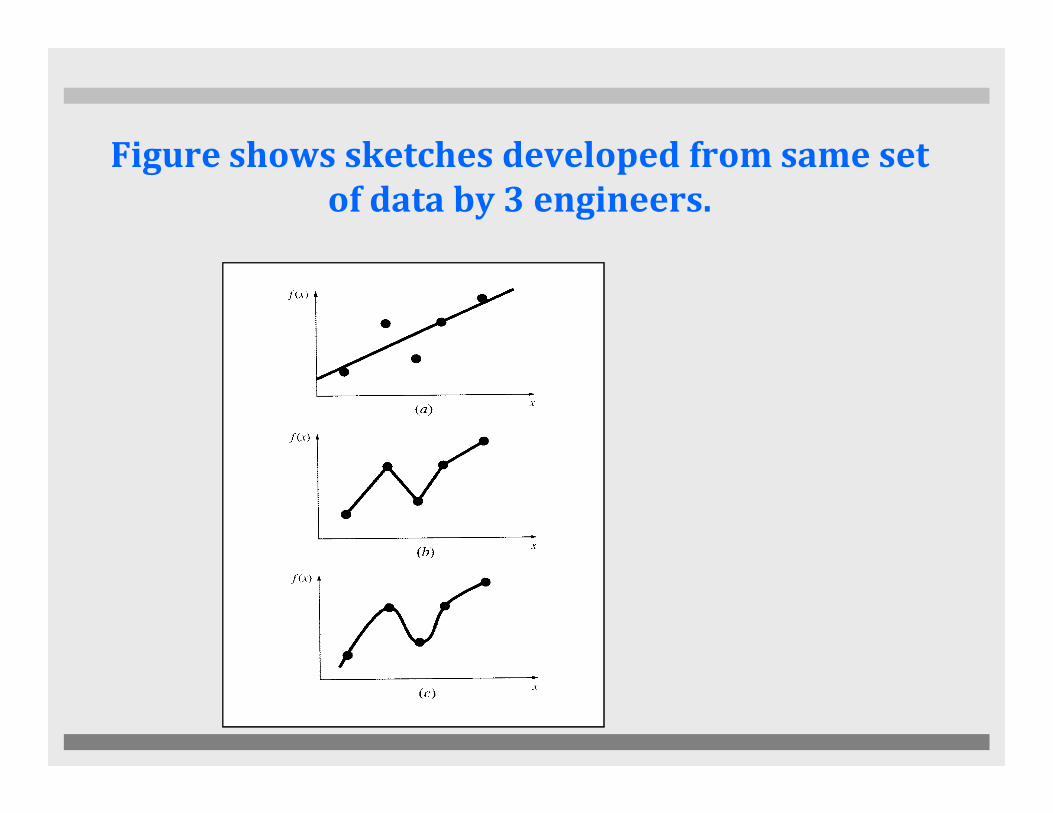
Figure shows sketches developed from same set

of data by 3 engineers.

a) least-squares regression - did not attempt to connect the point, but characterized the general upward trend of the data with a straight line

b) Linear interpolation - Used straight-line segments or linear interpolation to connect the points. Very common practice in engineering. If the values are close to being linear, such approximation provides estimates that are adequate for many engineering adequate for many engineering calculations. However, if the data is widely spaced, significant errorscan be introduced by such linear interpolation.

c) Curvilinear interpolation - Used curves to try to capture suggested by the data.

� Our goal here to develop systematic and objective method deriving such curves.

a) Least-square Regression

: i) Linear Regression

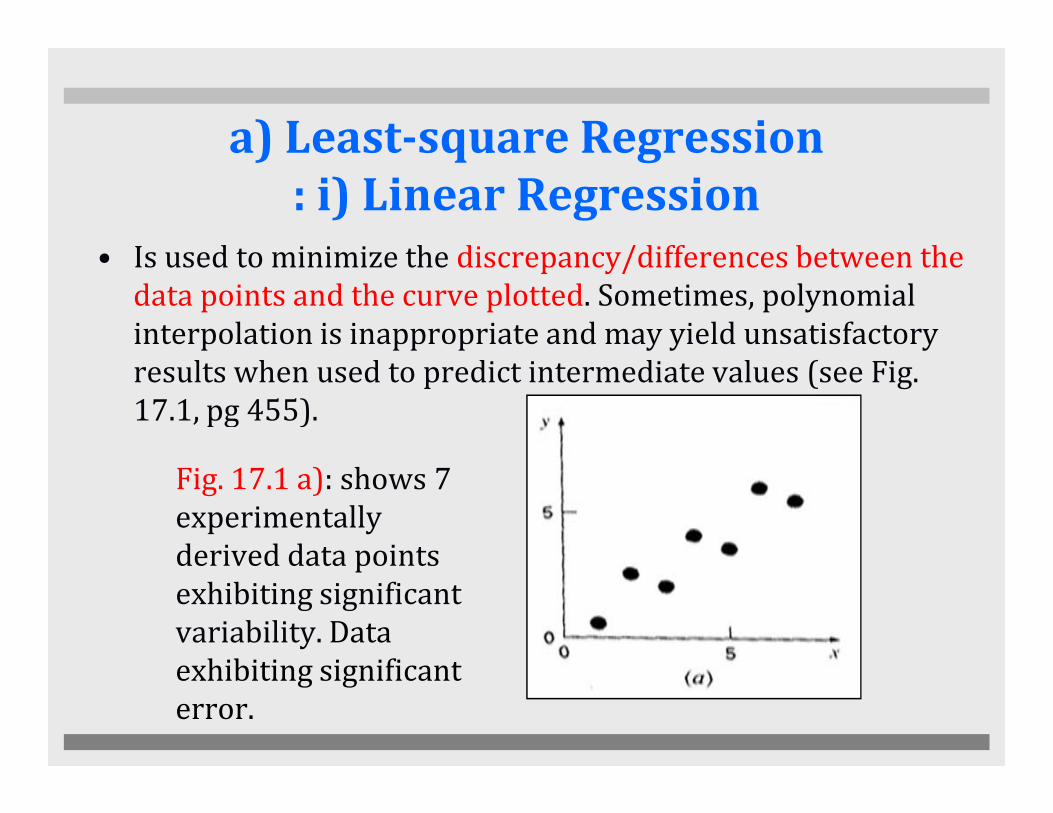
• Is used to minimize the discrepancy/differences between the

data points and the curve plotted. Sometimes, polynomial

interpolation is inappropriate and may yield unsatisfactory

results when used to predict intermediate values (see Fig.

17.1, pg 455).17.1, pg 455).

Fig. 17.1 a): shows 7

experimentally

derived data points

exhibiting significant

variability. Data

exhibiting significant

error.

Curve Fitting

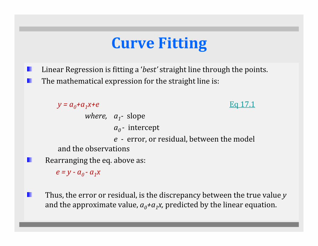
Linear Regression is fitting a ‘best’ straight line through the points.

The mathematical expression for the straight line is:

y = a0+a1x+e Eq 17.1

where, a1- slope

a - intercepta0 - intercept

e - error, or residual, between the model

and the observations

Rearranging the eq. above as:

e = y - a0 - a1x

Thus, the error or residual, is the discrepancy between the true value y

and the approximate value, a0+a1x, predicted by the linear equation.

Criteria for a ‘best’ Fit

• To know how a “best” fit line through the data is by minimize the sum

of residual error, given by ;

where; n : total number of points

∑∑==

−−=n

i

ii

n

i

i xaaye1

10

1

)( ----- Eq 17.2

• A strategy to overcome the shortcomings: The sum of the squares of

the errors between the measured y and the y calculated with the linear

model is shown in Eq 17.3;

∑ ∑∑= ==

−−=−==n

i

n

i

iielimeasuredi

n

i

ir xaayyyeS1 1

2

10

2

mod,,

1

2 )()(----- Eq 17.3

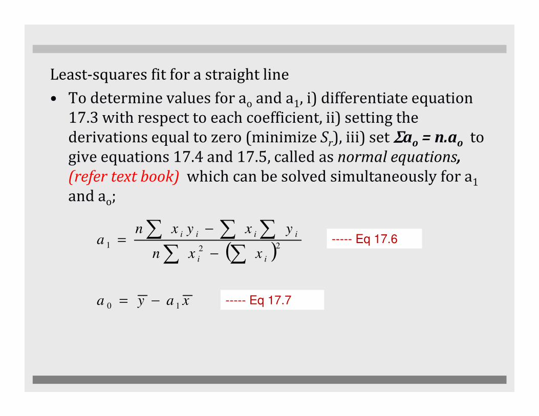
Least-squares fit for a straight line

• To determine values for ao and a1, i) differentiate equation

17.3 with respect to each coefficient, ii) setting the

derivations equal to zero (minimize Sr), iii) set ΣΣΣΣao = n.ao to

give equations 17.4 and 17.5, called as normal equations,

(refer text book) which can be solved simultaneously for a1

and ao;

( )

xaya

xxn

yxyxna

ii

iiii

10

221

−=

−

−=

∑ ∑∑ ∑ ∑

----- Eq 17.6

----- Eq 17.7

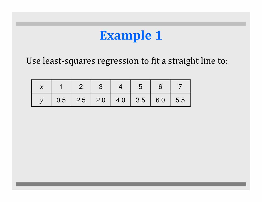
Example 1

Use least-squares regression to fit a straight line to:

x 1 2 3 4 5 6 7

y 0.5 2.5 2.0 4.0 3.5 6.0 5.5y 0.5 2.5 2.0 4.0 3.5 6.0 5.5

• Two criteria for least-square regression will provide the best estimates

of ao and a1 called maximum likelihood principle in statistics:

i. The spread of the points around the line of similar magnitude along

the entire range of the data.

ii. The distribution of these points about the line is normal.

• If these criteria are met, a “standard deviation” for the regression line

is given by equation:

---------- Eq. 17.9

sy/x : standard error of estimate

“y/x” : predicted value of y corresponding to a particular value of x

n -2 : two data derived estimates ao and a1 were used to compute Sr

(we have lost 2 degree of freedom)

2−=

n

SS r

xy

• Equation 17.9 is derived from Standard Deviation (Sy)

about the mean :

-------- (PT5.2, pg 442 )

-------- (PT5.3, pg 442 )

1−=

n

SS t

y

∑ −= 2)( yyS it

St : total sum of squares of the residuals between data

points and the mean.

• Just as the case with the standard deviation, the

standard error of the estimate quantifies the spread of

the data.

∑

Estimation of error in summary1. Standard Deviation

2. Standard error of the estimate

∑ −=

−=

2)(

1

yyS

n

SS

it

ty

----- (PT5.2, pg 442 )

----- (PT5.3, pg 442 )

2. Standard error of the estimate

where, y/x designates that the error is for a predict value of y

corresponding to a particular value of x.

2

)(1 1

2

10

2

−=

−−==∑ ∑= =

n

rS

S

xaayeiS

xy

n

i

n

iir

----- Eq 17.8

----- Eq 17.9

3. Determination coefficient

t

rt

S

SSr

−=2 ----- Eq 17.10

4. Correlation coefficient

∑ ∑ ∑ ∑

∑ ∑ ∑−−

−=

−=

2222 )()(

))((@

iiii

iiii

t

rt

yynxxn

yxyxnr

S

SSr ----- Eq 17.11

Example 2


x 1 2 3 4 5 6 7

y 0.5 2.5 2.0 4.0 3.5 6.0 5.5

Compute the standard deviation (Sy), the standard error

of estimate (Sy/x) and the correlation coefficient (r) for

data above (use Example 1 result)

Work with your buddy and lets do

Quiz 1


Compute the standard error of estimate (Sy/x) and the

correlation coefficient (r)

x 1 2 3 4 5 6 7 8 9

y 1 1.5 2 3 4 5 8 10 13

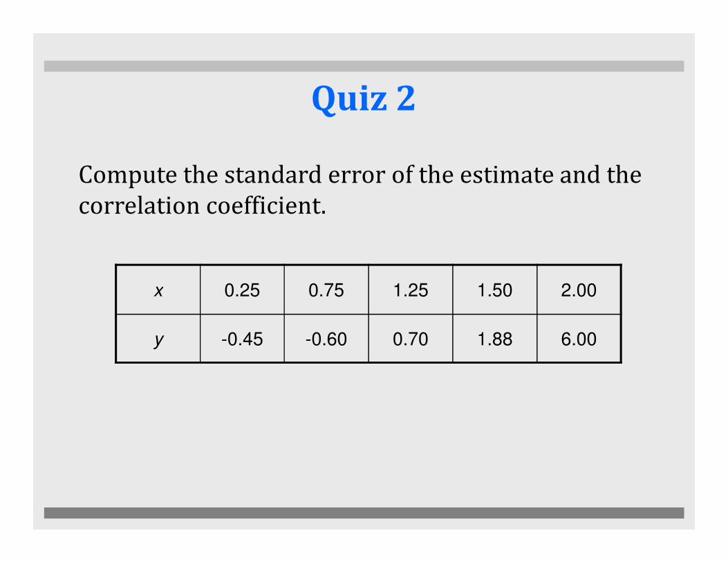
Quiz 2

Compute the standard error of the estimate and the

correlation coefficient.

x 0.25 0.75 1.25 1.50 2.00x 0.25 0.75 1.25 1.50 2.00

y -0.45 -0.60 0.70 1.88 6.00

Linearization of Nonlinear

Relationships

• Linear regression provides a powerful

technique for fitting the best line to data, where

the relationship between the dependent and the relationship between the dependent and

independent variables is linear.

• But, this is not always the case, thus first step in

any regression analysis should be to plot and

visually inspect whether the data is a linear

model or not.

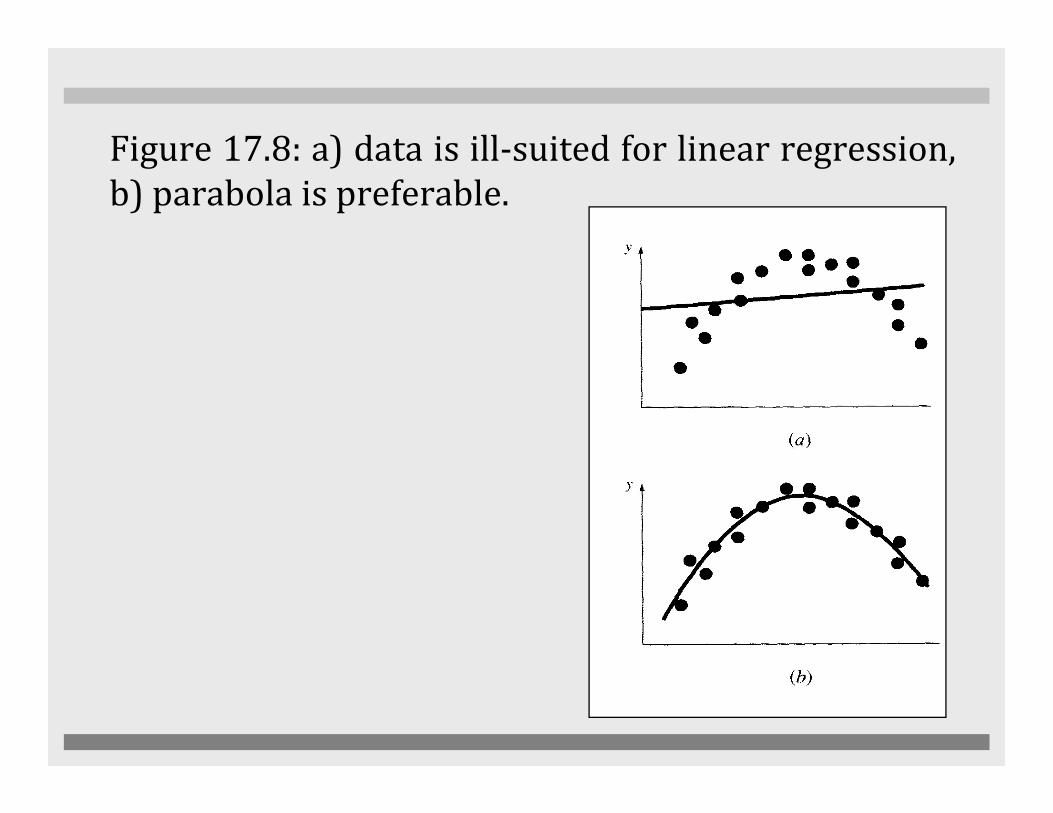
Figure 17.8: a) data is ill-suited for linear regression,

b) parabola is preferable.

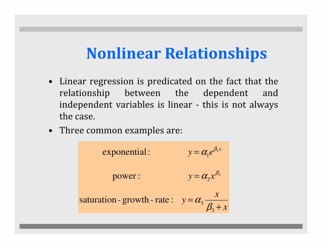
• Linear regression is predicated on the fact that the

relationship between the dependent and

independent variables is linear - this is not always

the case.

Nonlinear Relationships

• Three common examples are:

exponential : y = α1eβ1x

power : y = α2xβ2

saturation - growth - rate : y = α3

x

β3 + x

• One option for finding the coefficients for a nonlinear fit is

to linearize it. For the three common models, this may

involve taking logarithms or inversion:


Relationships

Model Nonlinear Linearized

exponential : y = α1eβ1x ln y = lnα1 + β1x

power : y = α2xβ2 log y = logα2 + β2 log x

saturation - growth - rate : y = α3

x

β3 + x

1

y=

1

α3

+β3

α3

1

x

• After linearization, Linear regression can be applied to

determine the linear relation.

• For example, the linearized exponential equation:


Relationships

xy ln ln βα += xy 11ln ln βα +=

y xa10a

Figure 17.9: Type of polynomial equations and their linearized

versions, respectively.

• Fig. 17.9, pg 453 shows population growth of radioactive

decay behavior.

Fig. 17.9 (a) : the exponential model

------ (17.12)xey 1

1

βα=

α1 , β1 : constants, β1 ≠ 0

This model is used in many fields of engineering to

characterize quantities.

Quantities increase : β1 positive

Quantities decrease : β1 negative

Fit an exponential model y = a ebx to:

x 0.4 0.8 1.2 1.6 2.0 2.3

y 750 1000 1400 2000 2700 3750

Example 2

Solution

• Linearized the model into;

ln y = ln a + bx

y = a0 + a1x ----- (Eq. 17.1)

• Build the table for the parameters used in eqs 17.6 and 17.7, as

in example 17.1, pg 444.

xi yi ln yi xi2 (xi)(ln yi)

0.4 750 6.620073 0.16 2.648029

0.8 1000 6.900775 0.64 5.520620

1.2 1400 7.244228 1.44 8.693074

1.6 2000 7.600902 2.56 12.161443

2.0 2700 7.901007 4.00 15.802014

2.3 3750 8.229511 5.29 18.927875

ΣΣΣΣ 8.38.38.38.3 44.49649644.49649644.49649644.496496 14.0914.0914.0914.09 63.75305563.75305563.75305563.753055

416083.76

496496.44ln383333.1

6

3.8

753055.63))(ln(09.14

496496.44ln3.8

6

1 1

2

11

====

==

==

=

∑ ∑

∑∑

= =

==

yx

yxx

yx

n

n

i

n

i

ii

n

i

i

n

i

i

i

843.0)3.8()09.14)(6(

)496496.44)(3.8()753055.63)(6(

)(

)(ln))(ln(

2

221

=−

−=

Σ−ΣΣΣ−Σ

==

b

xxn

yxyxnba

ii

iiii

25.6ln

)383333.1)(843.0(416083.7lnln0

=

−=−==

a

xbyaa

xy

bxay

843.025.6ln

lnln

+=∴

+=

bxeay =

51825.6ln 25.6 ==⇒= eaa

xbxeeay

843.0518==∴

Straight-line:

Exponential:

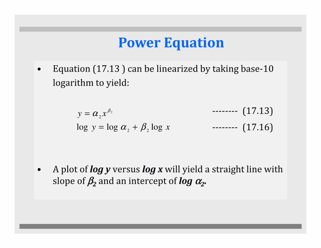
Power Equation

• Equation (17.13 ) can be linearized by taking base-10

logarithm to yield:

-------- (17.13)

-------- (17.16)xy

xy

logloglog

2

2

βα

α β

+=

=

-------- (17.16)

• A plot of log y versus log x will yield a straight line with

slope of ββββ2 and an intercept of log αααα2.

xy logloglog22

βα +=

Example 4

Linearization of a Power equation and fit equation

(17.13) to the data in table below using a logarithmic

transformation of the data.

x 1 2 3 4 5

y 0.5 1.7 3.4 5.7 8.4

xi yi log xi log yi (log xi)2 (log xi)(log yi)

1 0.5 0 -0.301 0 0

2 1.7 0.301 0.226 0.090601 0.068026

3 3.4 0.477 0.534 0.227529 0.2547183 3.4 0.477 0.534 0.227529 0.254718

4 5.7 0.602 0.753 0.362404 0.453306

5 8.4 0.699 0.922 0.488601 0.644478

ΣΣΣΣ 2.079 2.134 1.169135 1.420528

4268.05

134.2log4158.0

5

079.2log

420528.1))(log(log169135.1)(log

134.2log079.2log

5

1 1

2

11

====

==

==

=

∑ ∑

∑∑

= =

==

yx

yxx

yx

n

n

i

n

i

iii

n

i

i

n

i

i

b =nΣ(log x i )(log y i ) − (Σ log x i )( Σ log y i )

nΣ(log x i )2 − (Σ log x i )

2

b =(5)(1.420528 ) − (2.079 )(2.134 )

(5)(1.169135 ) − (2.079 ) 2= 1.75

xy

xbay

log75.13.0log

logloglog

+−=∴

+=

3.0ln

)4158.0)(75.1(4268.0)(logloglog

−=

−=−=

a

xbya

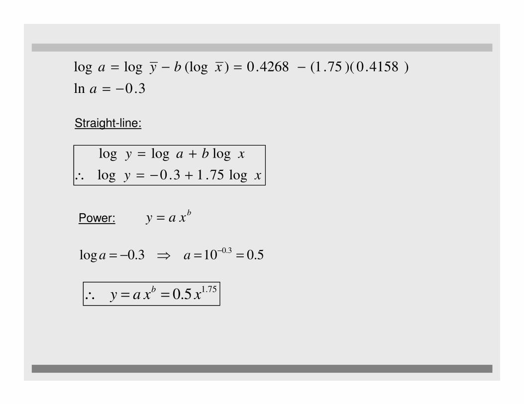
Straight-line:

bxay =

5.0103.0log 3.0 ==⇒−= −aa

75.15.0 xxayb ==∴

Power:

• Fig. 17.10 a), pg 455, is

a plot of the original

data in its

untransformed state,

while fig. 17.10 b) is a

plot of the transformed

data.

• The intercept, log α = • The intercept, log α2 =

-0.300, and by taking

the antilogarithm, α2

= 10-0.3 = 0.5.

• The slope is β2 = 1.75,

consequently, the

power equation is : y

= 0.5x1.75

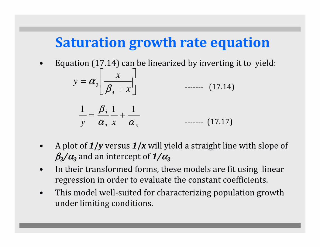
Saturation growth rate equation

• Equation (17.14) can be linearized by inverting it to yield:

------- (17.14)

------- (17.17)33

3111

ααβ

+=xy

+=

x

xy

3

3 βα

------- (17.17)

• A plot of 1/y versus 1/x will yield a straight line with slope of

ββββ3/αααα3 and an intercept of 1/αααα3

• In their transformed forms, these models are fit using linear

regression in order to evaluate the constant coefficients.

• This model well-suited for characterizing population growth

under limiting conditions.

33αα xy

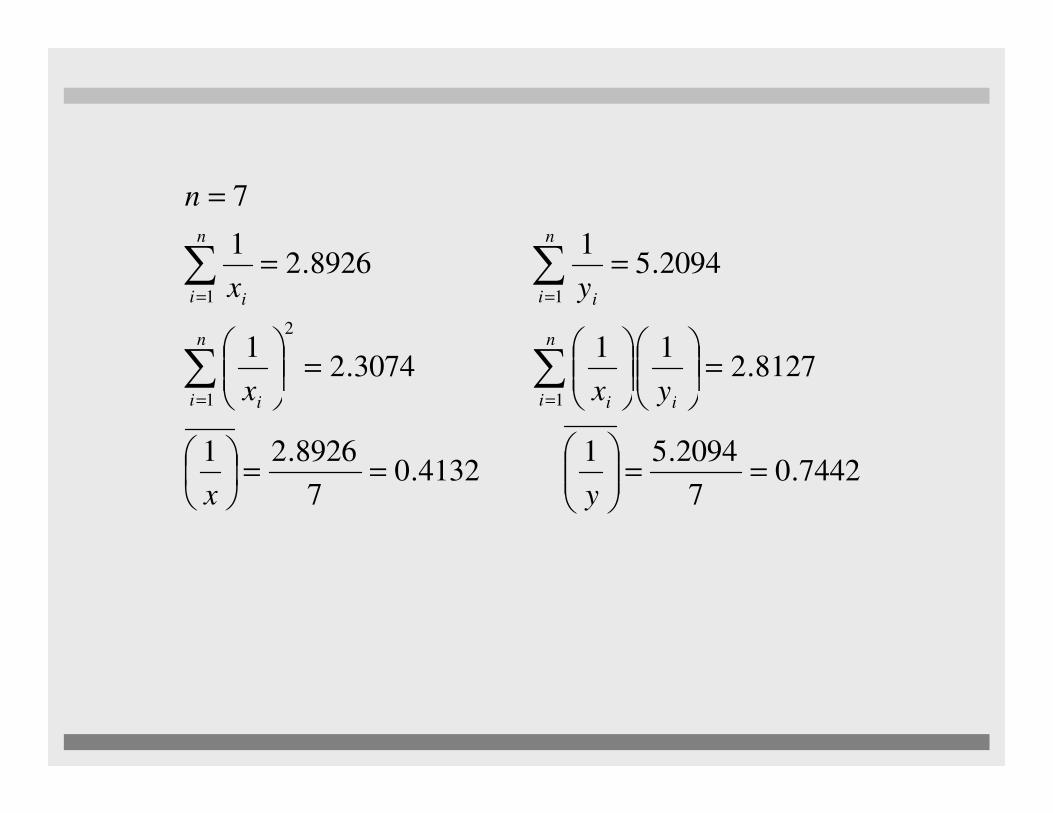
Example 5

Linearization of a saturation-growth

rate equation to the data in table below.

x 0.75 2 2.5 4 6 8 8.5

y 0.8 1.3 1.2 1.6 1.7 1.8 1.7

8127.211

3074.21

2094.51

8926.21

7

1 1

2

11

=

=

==

=

∑ ∑

∑∑

= =

==

yxx

yx

n

n

i

n

i iii

n

i i

n

i i

7442.07

2094.514132.0

7

8926.21

1 1

==

==

= =

yx

i i iii

xi yi 1/ xi 1/ yi (1/xi)2 (1/ xi)(1/yi)

0.75 0.8 1.33333 1.25000 1.7777 1.6666

2 1.3 0.50000 0.76923 0.2500 0.3846

2.5 1.2 0.40000 0.83333 0.1600 0.3333

4 1.6 0.25000 0.62500 0.0625 0.1562

6 1.7 0.16667 0.58823 0.0278 0.0981

8 1.8 0.12500 0.55555 0.0156 0.0694

8.5 1.7 0.11765 0.58823 0.0138 0.10458.5 1.7 0.11765 0.58823 0.0138 0.1045

ΣΣΣΣ 2.89260 5.20940 2.3074 2.8127

5935.0)8926.2()3074.2)(7(

)2094.5)(8926.2()8127.2)(7(

)1

(1

1111

2

2

2

=−

−=

Σ−

Σ

Σ

Σ−

Σ

=

a

b

xxn

yxyxn

a

b

ii

iiii

4990.01

)4132.0)(5935.0(7442.0111

=

−=

−

=

a

xa

b

ya

xa

b

ay

111+=

xy

15935.04990.0

1+=∴

Straight-line:

xy

+=

xb

xay

187.1)2)(5935.0(5935.0

24990.01

==∴⇒=

=∴⇒=

ba

b

aa

+=∴

x

xy

187.12

Saturation-growth:

Lets do Quiz 3

Fit a power equation and saturation

growth rate equation to:

x 1 2 3 4 5 6 7x 1 2 3 4 5 6 7

y 2.1 2.2 2.3 2.4 2.5 2.6 2.7

Figure 17.8: a) data is ill-suited for linear regression, b) parabola is preferable.

Polynomial Regression

• Another alternative is to fit polynomials to the data using

polynomial regression.

• The least-squares procedure can be readily extended to fit the

data to a higher-order polynomial.

• For example, to fit a second–order polynomial or quadratic:

• The sum of the squares of the residual is:

where n= total number of points

∑=

−−−=n

i

iiir xaxaayS1

22

210 )(

exaxaay +++= 2

210

• Then, taking the derivative of equation (17.18) with respect to each of the unknown coefficients, ao , a1 ,and, a2 of the polynomial, as in:

∑

∑

−−−−=

−−−−=

)(2

)(2

2

210

1

2

210

0

iiiir

iiir

S

xaxaayxa

S

xaxaaya

S

δ

δδ

δδ

• Setting the equations equal to zero and rearrange to develop set of normal equations and by setting ΣΣΣΣao = n.ao

∑ ∑ ∑ ∑∑ ∑ ∑ ∑

∑ ∑ ∑

=++

=++

=++

iiiii

iiiii

iii

yxaxaxax

yxaxaxax

yaxaxan

2

2

4

1

3

0

2

2

3

1

2

0

2

2

10

)()()(

)()()(

)()()(

∑ −−−−= )(2 2

210

2

2

iiiir xaxaayx

a

S

δδ

----- 17.19

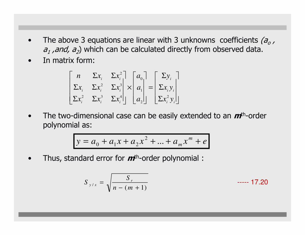
• The above 3 equations are linear with 3 unknowns coefficients (ao , a1 ,and, a2) which can be calculated directly from observed data.

• In matrix form:

• The two-dimensional case can be easily extended to an mth-order

Σ

Σ

Σ

=

×

ΣΣΣ

ΣΣΣ

ΣΣ

ii

ii

i

iii

iii

ii

yx

yx

y

a

a

a

xxx

xxx

xxn

2

2

1

0

432

32

2

• The two-dimensional case can be easily extended to an m -order polynomial as:

• Thus, standard error for mth-order polynomial :

exaxaxaaym

m +++++= ...2

210

)1(/ +−

=mn

SS r

xy ----- 17.20

Example 6Fit a second order polynomial to the data in the first 2 columns of

table 17.4:

xi yi xi2 xi

3 xi4 xi yi xi

2 yi

0 2.1 0 0 0 0 0

1 7.7 1 1 1 7.7 7.7

2 13.6 4 8 16 27.2 54.4

• From the given data:

m = 2 Σxi = 15 Σ xi4 = 979 y = 25.433

n = 6 Σ yi = 152.6 Σ xiyi = 585.6 Σ xi3 = 225

x = 2.5 Σ xi2 = 55 Σ xi

2yi = 2488.8

3 27.2 9 27 81 81.6 244.8

4 40.9 16 64 256 163.6 654.4

5 61.1 25 125 625 305.5 1527.5

ΣΣΣΣ 15 152.6 55 225 979 585.6 2488.8

• Therefore, the simultaneous linear equations are:

• Solving these equations through a technique such as Gauss

Σ

Σ

Σ

=

×

ΣΣΣ

ΣΣΣ

ΣΣ

ii

ii

i

iii

iii

ii

yx

yx

y

a

a

a

xxx

xxx

xxn

2

3

1

0

432

32

2

=

8.2488

6.585

6.152

97922555

2255515

55156

2

1

a

a

ao

• Solving these equations through a technique such as Gauss

elimination gives:

ao = 2.47857, a1 = 2.35929, and a2 = 1.86071

• Therefore, the least-squares quadratic equation for this

case is:

y = 2.47857 + 2.35929x + 1.86071x2

• To calculate st and sr , build table 17.4 for columns 3 and

4.

xi yi (yi- y )2 (yi-ao-a1xi-a2xi2)2

0 2.1 544.44 0.14332

1 7.7 314.47 1.00286

2 13.6 140.03 1.08158

3 27.2 3.12 0.80491

4 40.9 239.22 0.61951

5 61.1 1272.11 0.09439

Σ 152.6 2513.39 3.74657

74657.3)(

39.2513)(

22

210 =−−−Σ=

=−Σ=

iiir

it

xaxaayS

yyS

The standard error (regression polynomial):

12.1)12(6

74657.3

)1(=

+−=

+−=

mn

SS r

xy

• The correlation coefficient can be calculated by using equations

17.10 and 17.11, respectively:

Therefore, r2 = (S – S ) / S = (2513.39 – 3.74657) / 2513.39

∑ ∑ ∑ ∑

∑ ∑ ∑−−

−=

−=

2222 )()(

))((@

iiii

iiii

t

rt

yynxxn

yxyxnr

S

SSr

t

rt

S

SSr

−=2

Therefore, r2 = (St – Sr) / St = (2513.39 – 3.74657) / 2513.39

r2 = 0.99851

∴The correlation coefficient is, r = 0.99925

• The results indicate that 99.851% of the original uncertainty has

been explained by the model. This result supports the conclusion

that the quadratic equation represents an excellent fit, as evident

from Fig.17.11.

Figure 17.11: fit of a second-order polynomial

TOPICS

Polynomial Interpolation (Linear interpolation, Quadratic Interpolation, Newton

DD)

Lagrange Interpolation

Spline Interpolation

Interpolation• Polynomial Interpolation is a common method to determine

intermediate values between data points.

• General equation for nth order polynomial is:

• Polynomial interpolation consists of determining the unique nth-order polynomial that fits n+1 data point.

• For n+1 data points, there is only one polynomial of order n that

n

n xaxaxaaxf +++= .....)( 2

210 ----- 18.1

• For n+1 data points, there is only one polynomial of order n that passes through all the points.

• For example, there is only one straight line (first-order polynomial) that connects two points (Fig. 18.1a) and only one parabola connects a set of three points (Fig.18.1b).

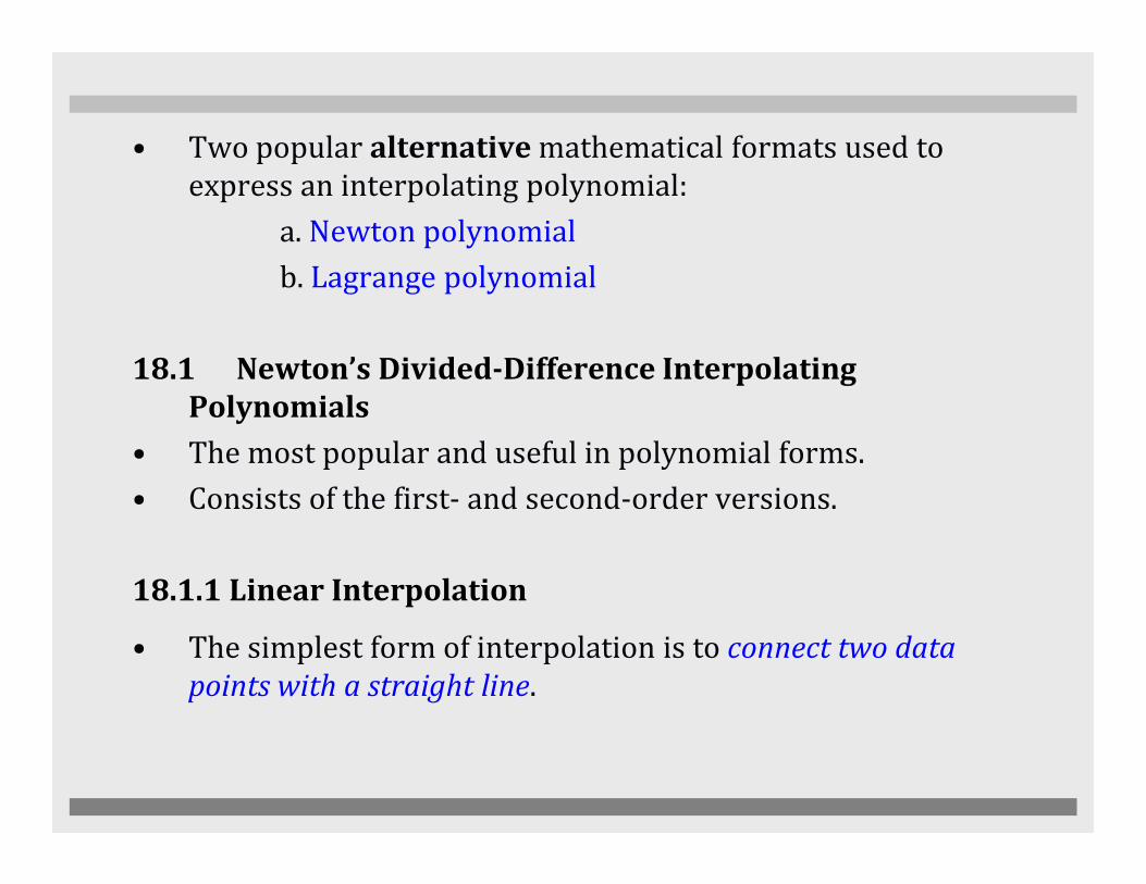
• Two popular alternative mathematical formats used to

express an interpolating polynomial:

a. Newton polynomial

b. Lagrange polynomial

18.1 Newton’s Divided-Difference Interpolating

Polynomials

• The most popular and useful in polynomial forms.• The most popular and useful in polynomial forms.

• Consists of the first- and second-order versions.

18.1.1 Linear Interpolation

• The simplest form of interpolation is to connect two data

points with a straight line.

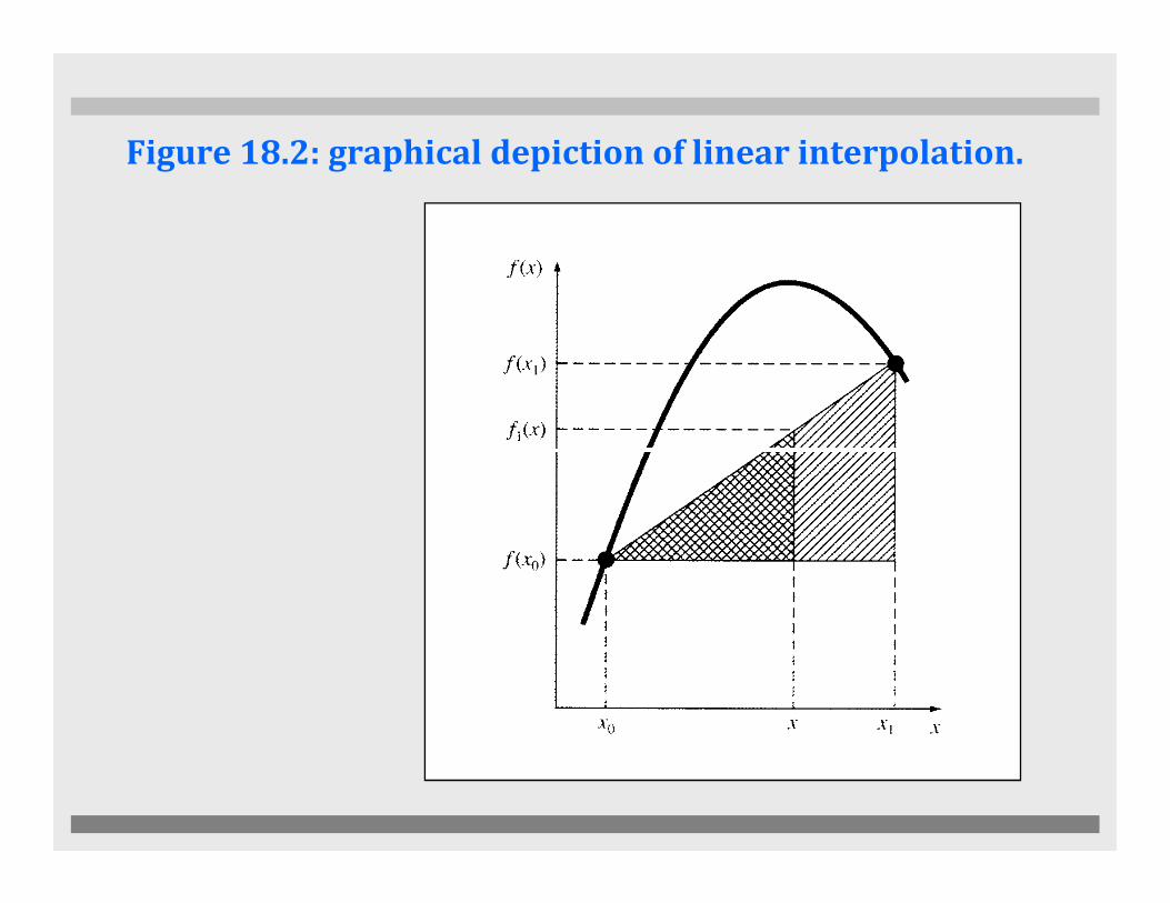
Figure 18.2: graphical depiction of linear interpolation.

• This linear interpolation technique can be depicted graphically as

shown in fig 18.2, in which, the similar triangles can be

rearranged to yield a linear-interpolation formula;

- f1(x) is refer to first order interpolation polynomial

)()()(

)()( 0

01

0101 xx

xx

xfxfxfxf −

−−

+= ----- 18.2

-The term is a finite-divided-difference

approximation of the first derivative.

• In general, the smaller the interval between the data points, the

better the approximation.

)()(

01

01

xx

xfxf

−−

Figure 18.2: graphical depiction of linear interpolation.

Example 7

Estimate the natural logarithm of 2 using linear

interpolation. First, perform the computation by

interpolating between ln 1 = 0 and ln 6 = 1.791759.

Then, repeat the procedure, but use a smaller interval

from ln 1 to ln 4 (1.386294). Note that the true valuefrom ln 1 to ln 4 (1.386294). Note that the true value

of ln 2 is 0.6931472.

Solution

By using equation (18.2), a linear interpolation for ln 2

from xo = 1 to x1 = 6 to give;

)()()(

)()( 001

01 xxxx

xfxfxfxf −

−−

+=

x f(x)

x0=1 f(x0) =0

x=2 f1(x)=?)()()( 0

01

01 xxxx

xfxf −−

+=

3583519.0)12(16

0791759.10)2(1 =−

−−

+=f

x1=6 f(x1)=1.791759

%3.48100*6931472.0

3583519.06931472.0=

−=

tε

• Then, using the smaller interval from xo = 1 to x1 = 4 yields;

x f(x)

x0=1 f(x0) =0

x=2 f1(x)=?

x1=4 f(x1)=1.386294

4620981.0)12(14

0386294.10)2(1 =−

−−

+=f

• Thus, using the shorter interval reduces the percent

relative error to εt = 33.3%.

• Both interpolations are shown in Fig.18.3, along with true

function.

%3.33100*6931472.0

4620981.06931472.0

14

=−

=

−

tε

Figure 18.3: Comparison of two linear interpolations

with different intervals.

Quiz 4

Estimate the logarithm of 5 to the base 10 (log5) using linear

interpolation.

a) Interpolate between log 4=0.60206 and log6=0.7781513

b) Interpolate between log4.5=0.6532125 and log

5.5=0.74036275.5=0.7403627

For each of the interpolations, compute the percent relative

error based on the true value

18.1.2 Quadratic Interpolation

The error in example 18.1 (linear interpolation) resulted from

approximation of a curve with a straight line.

With 3 data points, the estimation can be improved with a

second-Order Polynomial (quadratic polynomial or

parabola). Thus;

----- (18.3)

Although equation (18.3) seem to differ from the general

polynomial (equation 18.1), the two equations are equivalent, by

multiplying the terms in equation (18.3) to yield;

f2(x) = bo + b1x – b1xo + b2x2 + b2xox1 – b2xxo – b2xx1

))(()()( 1020102 xxxxbxxbbxf −−+−+=

or in collecting terms,

f2(x) = ao + a1x + a2x2

where;

ao = bo – b1xo + b2xox1

a1 = b1 – b2xo – b2x1

a2 = b2

• Thus, equations 18.1 and 18.3 are alternative, equivalent formulations of

the unique second-order polynomial joining three points.

• To determine the values of coefficient (bo, b1, and, b2), rearrange and use

Eq 18.3, substitute Eq 18.4 into 18.3, and substitute Eq 18.4 and 18.5 into

Eq 18.3 to yield Eq 18.6.

02

01

01

12

12

2

01

011

00

)()()()(

)()(

)(

xx

xx

xfxf

xx

xfxf

b

xx

xfxfb

xfb

−−−

−−−

=

−−

=

= ----- 18.4

----- 18.5

----- 18.6

Example 8

Fit a second-order polynomial to the three points

used in linear interpolation example

xo = 1 f(x0) = 0xo = 1 f(x0) = 0

x1 = 4 f(x1) =1.386294

x2 = 6 f(x2) =1.791759

Use the polynomial to evaluate ln 2

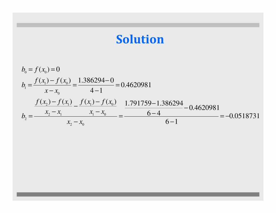
Solution

4620981.0386294.1791759.1)()()()(

4620981.014

0386294.1)()(

0)(

0112

0

01

1

00

−−

−−

−−−

=−

−=

−−

=

==

xfxfxfxf

xx

xfxfb

xfb

0518731.016

4620981.046

386294.1791759.1

02

0112

2−=

−

−−−

=−

−−

−=

xx

xxxxb

Substituting these values into equation 18.3 yields the

quadratic formula:

f2(x) = bo + b1(x – xo) + b2(x – xo)(x – x1)

f2(x) = 0 + 0.462098(x – 1) – 0.0518731(x – 1)(x – 4)

which can be evaluated at x = 2 for;

f (2) = 0.5658444f2(2) = 0.5658444

which represents a relative error of εt = 18.4%.

• Thus, the curvature introduced by the quadratic

formula (Fig.18.4) improves the interpolation

compared with the result obtained using straight lines

in example 18.1, Fig.18.3.

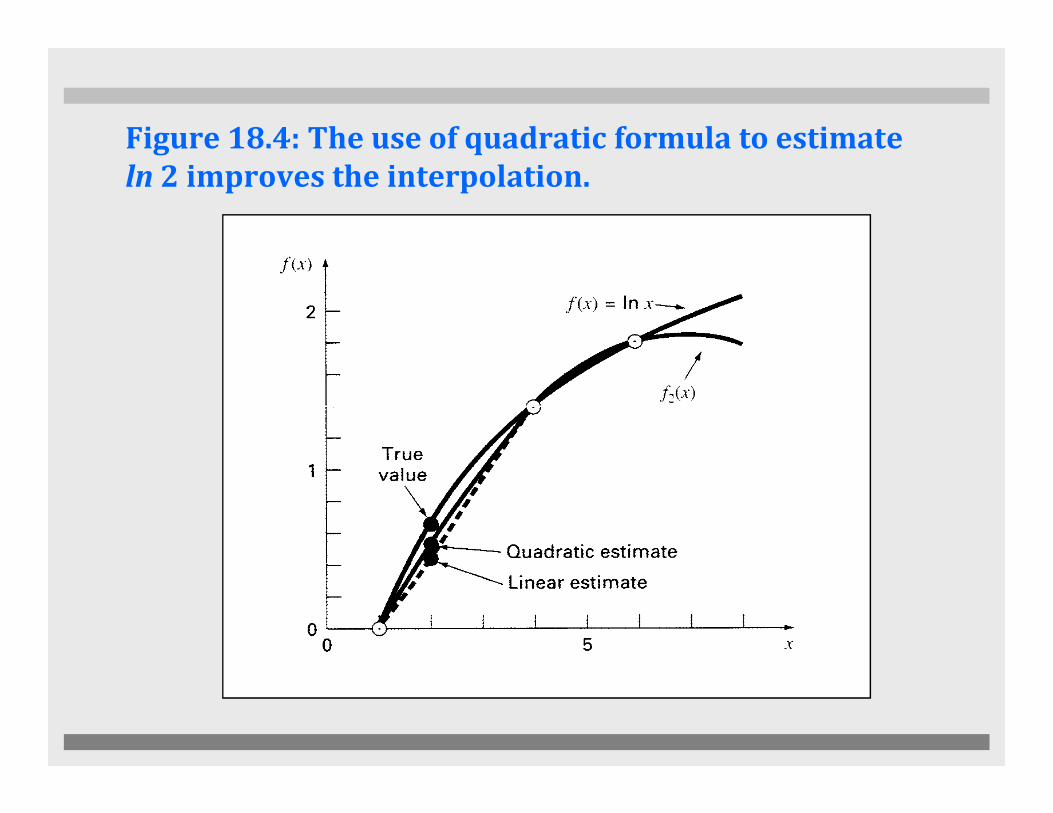
Figure 18.4: The use of quadratic formula to estimate

ln 2 improves the interpolation.

Example 9

Given the data, calculate f(3.4) using Newton’s

polynomials of order 1 to 2.

x 1 2 2.5 3 4 5

f(x) 1 5 7 8 2 1

3.4

Solution

1)( 5

7)(5.2

2)(4

8)(3

22

22

11

00

=⇒=

=⇒=

=⇒=

=⇒=

xfx

or

xfx

xfx

xfx

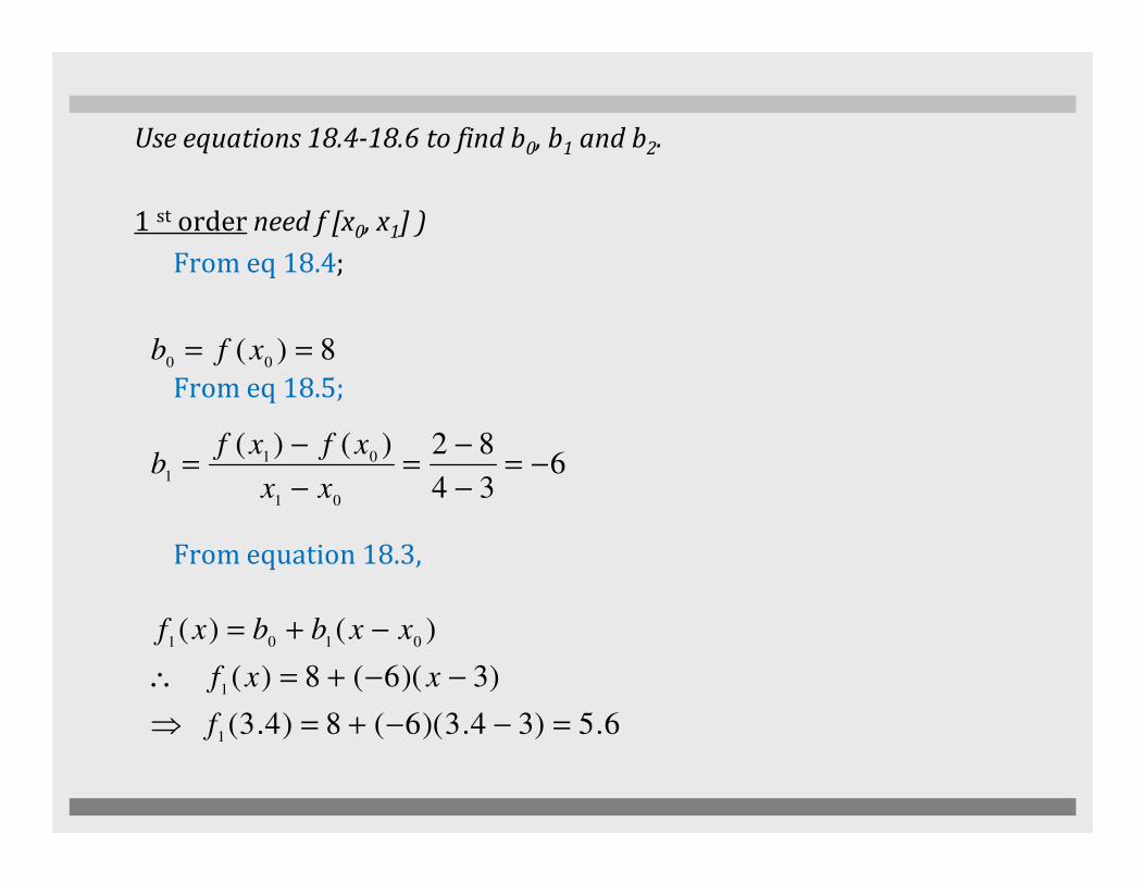
Use equations 18.4-18.6 to find b0, b1 and b2.

1 st order need f [x0, x1] )

From eq 18.4;

From eq 18.5;

82)()(

8)(00

−=−

=−

=

==

xfxf

xfb

From equation 18.3,

6.5)34.3)(6(8)4.3(

)3)(6(8)(

)()(

634

82)()(

1

1

0101

01

01

1

=−−+=⇒

−−+=∴

−+=

−=−−

=−−

=

f

xxf

xxbbxf

xx

xfxfb

2nd order (need f [x0, x1, x2] )

From equation 18.6;

From eq 18.3 for 2nd order

75.535.2

)6(45.2

27)()()()(

02

01

01

12

12

2−=

−

−−−

−

=−

−−

−−−

=xx

xx

xfxf

xx

xfxf

b

From eq 18.3 for 2nd order

98.6)4.3(

)44.3)(34.3)(75.5()34.3)(6(8)4.3(

)4)(3)(75.5()3)(6(8)(

))(()()(

2

2

2

1020102

=

−−−+−−+=⇒

−−−+−−+=∴

−−+−+=

f

f

xxxxf

xxxxbxxbbxf

Quiz 5

x 1 2 3 5 6

f(x) 4.75 4 5.25 19.75 36

Given the data, calculate f(4) using Newton’s

polynomial of order 1 to 2

f(x) 4.75 4 5.25 19.75 36

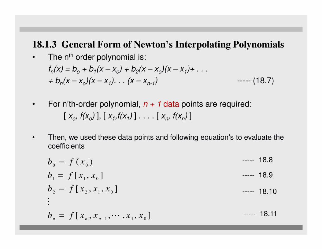
18.1.3 General Form of Newton’s Interpolating Polynomials

• The nth order polynomial is:

fn(x) = bo + b1(x – xo) + b2(x – xo)(x – x1)+ . . .

+ bn(x – xo)(x – x1). . . (x – xn-1) ----- (18.7)

• For n’th-order polynomial, n + 1 data points are required:

[ xo, f(xo) ], [ x1,f(x1) ] . . . . [ xn, f(xn) ]

• Then, we used these data points and following equation’s to evaluate the coefficients

],,,,[

],,[

],[

)(

011

0122

011

00

xxxxfb

xxxfb

xxfb

xfb

nnnL

M

−=

=

=

= ----- 18.8

----- 18.9

----- 18.10

----- 18.11

• Where the bracketed [ ] function evaluations are finite

divided differences (FDD);

• For example, the first finite divided difference is

represented generally as;

ji

ji

jixx

xfxfxxf

−

−=

)()(],[ ----- 18.12

• Similarly, the n’th finite divided difference is

ki

kjji

kjixx

xxfxxfxxxf

−

−=

],[],[],,[

difference divided finite Second

----- 18.13

0

02111

011

],[],[],,[

xx

xxxfxxxfxxxxf

n

nnnn

nn −−

= −−−−

LLL ----- 18.14

• These differences can be used to evaluate the coefficients

in equations (18.8) through (18.11), which can then

substituted into equation (18.7) to yield the interpolating

polynomial, called as Newton’s divided-difference

interpolating polynomial;

[ ] [ ]( ) [ ]01110

012100100

,....,,)...)((....

,,))((,)()()(

xxxfxxxxxx

xxxfxxxxxxfxxxfxf

nnn

n

−−−−−++

−−+−+=----- 18.15

Example 10

From example 18.2, data points at x0=1, x1=4 and x2=6 were

used to estimate ln 2 with a parabola. Now adding a fourth

point (x3=5; f(x3)=1.609438), Estimate ln 2 with a third order

Newton’s interpolating Polynomial.

x0=1 x1=4 x2=6 x3=5

f(x0)=0 f(x1)=1.386294 f(x2)=1.791759 f(x3)=1.609438

Solution

The third-order polynomial with n = 3 is,

f3(x) = bo + b1(x – xo) + b2(x – xo)(x – x1) + b3(x – xo)(x – x1)(x-x2)

The first divided differences are (use eq 18.12):

4620981.014

0386294.1)()(],[

01

0101 =

−−

=−−

=xx

xfxfxxf

The second divided differences (use equation 18.13):

2027326.046

386294.1791759.1)()(],[

12

1212 =

−−

=−−

=xx

xfxfxxf

1823216.065

386294.1609438.1)()(],[

23

2323 =

−−

=−−

=xx

xfxfxxf

02041100.045

2027326.01823216.0],[],[],,[

13

1223

123−=

−−

=−−

=xx

xxfxxfxxxf

05187311.016

4620981.02027326.0],[],[],,[

02

0112

012−=

−−

=−−

=xx

xxfxxfxxxf

The third divided differences:

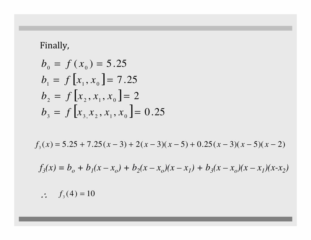
Finally, using eqs 18.8-18.11:

007865529.0],,,[

15

)05187311.0(02041100.0],,[],,[],,,[

0123

03

012123

0123

=

−−−−

=−−

=

xxxxf

xx

xxxfxxxfxxxxf

b0 = f ( x 0 ) = 0

b1 = f x1, x 0[ ] = 0.4620981

Insert all values into eqs 18.7;

, which represents a relative error of εt = 9.3%.

1 1 0[ ]b2 = f x 2 , x1, x 0[ ] = −0.05187311

b3 = f x 3,x 2 , x1, x 0[ ] = 0.007865529

)6)(4)(1(007865529.0

)4)(1(05187311.0)1(4620981.00)(3

−−−+

−−−−+=

xxx

xxxxf

6287686.0)2(3 =f

Quiz 6

Calculate f (4) with a third and fourth order Newton’s

interpolating polynomial.

x 1 2 3 5 6

f(x) 4.75 4 5.25 19.75 36

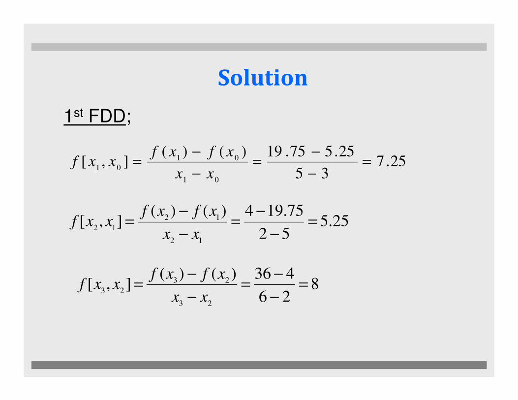
Solution

1st FDD;

25.735

25.575.19)()(],[

01

01

01=

−−

=−−

=xx

xfxfxxf

25.552

75.194)()(],[

12

12

12=

−−

=−−

=xx

xfxfxxf

826

436)()(],[

23

23

23=

−−

=−−

=xx

xfxfxxf

2nd FDD

232

25.725.5],[],[],,[

02

0112

012=

−−

=−−

=xx

xxfxxfxxxf

75.256

25.58],[],[],,[

13

1223

123=

−−

=−−

=xx

xxfxxfxxxf

3rd FDD

25.0],,,[

36

275.2],,[],,[],,,[

0123

03

012123

0123

=

−−

=−−

=

xxxxf

xx

xxxfxxxfxxxxf

Finally,

[ ][ ][ ] 25.0,,

2,,

25.7,

25.5)(

012,33

0122

011

00

==

==

==

==

xxxxfb

xxxfb

xxfb

xfb

f3(x) = bo + b1(x – xo) + b2(x – xo)(x – x1) + b3(x – xo)(x – x1)(x-x2)

∴

)2)(5)(3(25.0)5)(3(2)3(25.725.5)(3

−−−+−−+−+= xxxxxxxf

10)4(3

=f

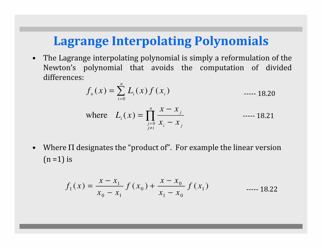
• The Lagrange interpolating polynomial is simply a reformulation of the

Newton’s polynomial that avoids the computation of divided

differences:

∏

∑

=

=

−

−=

=

n

jji

j

i

n

iiin

xx

xxxL

xfxLxf

0

0

)( where

)()()( ----- 18.20

----- 18.21

Lagrange Interpolating Polynomials

• Where Π designates the “product of”. For example the linear version

(n =1) is

≠= −

ijj

jixx0

)()()( 1

01

00

10

11 xf

xx

xxxf

xx

xxxf

−−

+−−

= ----- 18.22

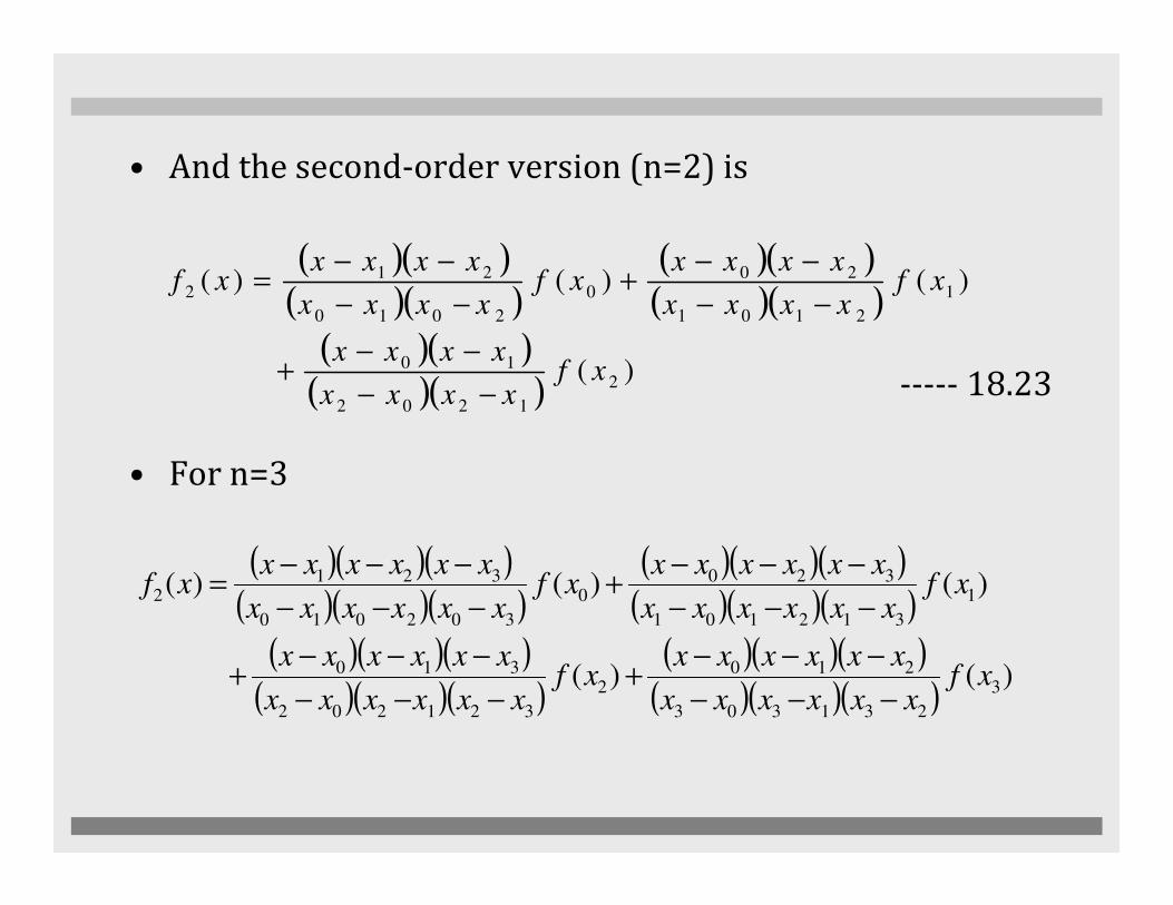
• And the second-order version (n=2) is

• For n=3

( )( )( )( )

( )( )( )( )

( )( )( )( )

)(

)()()(

2

1202

10

1

2101

200

2010

212

xfxxxx

xxxx

xfxxxx

xxxxxf

xxxx

xxxxxf

−−−−

+

−−−−

+−−

−−=

----- 18.23

• For n=3

( )( )( )( )( )( )

( )( )( )( )( )( )

( )( )( )( )( )( )

( )( )( )( )( )( )

)()(

)()()(

3

231303

2102

321202

310

1

312101

3200

302010

3212

xfxxxxxx

xxxxxxxf

xxxxxx

xxxxxx

xfxxxxxx

xxxxxxxf

xxxxxx

xxxxxxxf

−−−−−−

+−−−

−−−+

−−−−−−

+−−−

−−−=

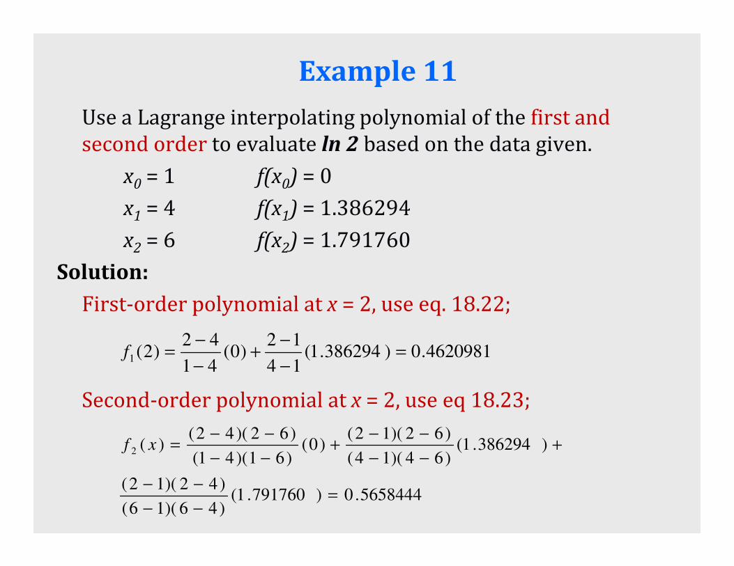
Example 11

Use a Lagrange interpolating polynomial of the first and

second order to evaluate ln 2 based on the data given.

x0 = 1 f(x0) = 0

x1 = 4 f(x1) = 1.386294

x2 = 6 f(x2) = 1.791760

Solution:Solution:

First-order polynomial at x = 2, use eq. 18.22;

Second-order polynomial at x = 2, use eq 18.23;

4620981.0)386294.1(14

12)0(

41

42)2(1 =

−−

+−−

=f

5658444.0)791760.1()46)(16(

)42)(12(

)386294.1()64)(14(

)62)(12()0(

)61)(41(

)62)(42()(2

=−−−−

+−−−−

+−−−−

=xf

Working with

your buddy to do Quiz 7

Quiz 7

Given the data, calculate f(4) using the Lagrange

polynomials of order 1 to 2.

x 1 2 3 5 6x 1 2 3 5 6

f(x) 4.75 4 5.25 19.75 36

Chapter 5Chapter 5Lets do past year

questions

Q1Q3Q6Q8

Assignment (please use excell)

Given the data below, use least squares regression to fit a) a

straight line b) a power equation c) a saturation-growth-rate

equation and d) a parabola. Find the r2 value and justify

which is the best equation to represent the data.

x 5 10 15 20 25 30 35 40 45 50

y 17 24 31 33 37 37 40 40 42 51

Lets do past year question - Q3 and Q6

Develop a MATHLAB program which can be written in a command window to solve this

problem which will give the linear regression problem which will give the linear regression equation

Lets try mathlab to solve linear

regression problem

T(oC) 4 8 12 16 20 24 28

V (10-2cm2/s) 1.88 1.67 1.49 1.34 1.22 1.11 1.02

Question?

THE END

Thank You for the Attention

chapter 5 - curve fitting · curve fitting linear regression is fitting a ‘best’ straight line...

Documents