chapter 5 - characteristic values from bayesian statistics...

JointTC205/TC304WorkingGroupon“Discussionofstatistical/reliabilitymethodsforEurocodes” –FinalReport(Sep2017)

1

Chapter 5 Selection of characteristic values for rock and soil properties

using Bayesian statistics and prior knowledge

Lead discusser:

Yu Wang

Discussers (alphabetical order):

Marcos Arroyo, Zijun Cao, Jianye Ching, Tim Länsivaara, Trevor Orr, Kok-Kwang Phoon,

Hansruedi Schneider, Brian Simpson

5.1 Introduction

Selection of design values for material properties is indispensable in engineering analyses and

designs. In many engineering disciplines (e.g., structural engineering), design values are

derived from characteristic values of material properties (e.g., concrete strength) which are

often determined using statistical methods. In geotechnical engineering, however, it has been

a challenging task to use statistical methods for determination of soil or rock property

characteristic values, because the number of soil/rock property data obtained during site

investigation is generally too sparse to generate meaningful statistics, i.e., the so-called “curse

of small sample size” (Phoon 2017). Engineering experience and judgment are often used to

supplement the limited measurement data during the selection of characteristic values for soil

or rock properties. A Bayesian framework may be used to integrate the limited measurement

data with engineering experience and judgment (as prior knowledge) in a rational and

quantitative manner. This has been recognized in Eurocode 7 (EC7 (e.g., CEN 2004)) and

referenced in the clause 2.4.5.2(10): “If statistical methods are employed in the selection of

characteristic values for ground properties, such methods should differentiate between local

and regional sampling and should allow the use of a priori knowledge of comparable ground

properties.” This preliminary report aims to provide a start-of-the-art review on the use of

Bayesian statistics and prior knowledge for selection of ground property characteristic values.

The report focuses on routine engineering practices on conventional types of geotechnical

structures with no exceptional risk or difficult ground or loading conditions (e.g., the

Geotechnical Category 2 in EC7). Some design examples of such category are given by Orr

(2005). Random field modeling of variability and uncertainty is not covered in this report.

5.2 Definition of characteristic value

The definition of characteristic value for ground properties itself might be an intriguing issue,

although detailed discussion on this issue is beyond the scope of this report and is referred to

Schneider and Schneider (2013) and Orr (2017) for the discussion associated with EC7.


2

There are different definitions of the characteristic value for ground properties in various

geotechnical design codes around the world. For example, a mean value is generally used as

nominal value (i.e., characteristic value) in several reliability-based design codes in North

America (e.g., Phoon et al. 2003a&b, Paikowsky et al. 2004&2010, Fenton et al. 2016). EC7

recommends that (see clause 2.4.5.2(2)) “characteristic value of a geotechnical parameter

shall be selected as a cautious estimate of the value affecting the occurrence of the limit

state.” It further notes that (see clause 2.4.5.2(11)) “If statistical methods are used, the

characteristic value should be derived such that the calculated probability of a worse value

governing the occurrence of the limit state under consideration is not greater than 5%.” A

note to this clause clarifies that “In this respect, a cautious estimate of the mean value is a

selection of the mean value of the limited set of geotechnical parameter values, with a

confidence level of 95%; where local failure is concerned, a cautious estimate of the low

value is a 5% fractile.” Although the above general statement describing the characteristic

value in EC7 is sensible, there is an under-stated difficulty in making this statement

sufficiently concrete for codification. Orr (2017) suggested that more guidance on the

selection of characteristic values is needed for reduce the spread of the selected characteristic

values and achieve designs with more consistent reliability.

Using 5% fractile, mean value or other percentage fractile as the characteristic value

has their respective pros and cons. Although using the 5% fractile has the advantages of

reflecting both the mean value and uncertainty (e.g., 5% fractile is equal to the mean value

minus 1.65 standard deviations for a normal distribution) and being in harmony with the

definition of the characteristics value for other engineering materials (e.g., concrete in

structural engineering), the 5% fractile is difficult to quantify due to the limited ground

property data obtained during a site investigation and often the large extent of the failure zone

compared to the number of test results. In contrast, although the mean value may be

estimated from limited ground property data with better accuracy than the 5% fractile, it does

not provide any indication of the variability and hence the uncertainty in the ground

properties. Therefore, the impact of different levels of ground property uncertainty on

geotechnical design should be considered by other means within the design codes. For

example, a three-tier system of different resistance factors for different levels of ground

property uncertainty is developed in some design codes (e.g., Phoon et al. 2003a&b, Fenton

et al. 2016, Phoon et al. 2016). Indeed, the definition of characteristic values for ground

properties and the calibration of load and resistance (or partial) factors are intrinsically linked

with each other. They should be compatible with each other and act together to properly

account for the impact of different levels of ground property uncertainty on geotechnical

design.

No matter how the characteristic value is defined for ground properties, quantification

of ground property uncertainty is essential. Bayesian methods described in the next section


3

not only effectively tackle the difficulty in dealing with limited site-specific ground property

data, but are also consistent with existing geotechnical practice (i.e., using engineering

experience and judgment together with limited site-specific measurement data).

5.3 Bayesian methods

Under a Bayesian framework, site information available prior to a project (e.g., existing data

in literature, engineering experience, and engineers’ expertise) may be used as “prior”

knowledge and integrated with limited project/site-specific measurement data in a rational

and quantitative manner (e.g., Wang et al. 2016a). Starting from the Bayes Theorem, Eq. (5-1)

can be derived to update statistical parameters P (e.g., mean and standard deviation

) of a design ground property XD (e.g., soil effective friction angle ’), which is treated as a

random variable, given a set of site-specific test data as (e.g., Ang and Tang 2007):

PPP PDataPKPriorDataP , (5-1)

where K is a normalizing constant independent of the statistical parameters P of XD; Data

= MX is the site-specific measurement data (e.g., a set of standard penetration test SPT-N

values); PP is the prior distribution of the statistical parameters in the absence of

site-specific measurement data; and PDataP = )|( PMXP is the likelihood function.

Two critical elements in the Bayesian framework are the formulations of prior distribution

(see Section 5.4) and the likelihood function described in this section.

The likelihood function )|( PMXP is a probability density function, PDF, of

site-specific measurement data MX for a given set of statistical parameters P . It

quantifies probabilistically the P information provided by MX . Formulation of the

likelihood function (i.e., )|( PMXP ) requires a likelihood model that probabilistically

describes the relationship between the statistical parameters P of a design property DX

and project-specific test data MX . Generally speaking, the likelihood model shall reflect

sound physical insights into the relationship between the design property DX and the

measurement data MX and the propagation of various uncertainties that occurred during


4

site characterization (e.g., Wang et al. 2016a). As much as possible insights from soil or rock

mechanics should be incorporated in the likelihood model. For example, insights from soil

mechanics suggest that undrained shear strength, Su, of clay is not a fundamental soil property,

but depends on the vertical effective stress, v’. It is therefore a better likelihood model to

consider Su/v’ than Su as a random variable (Cao and Wang 2014). In addition, the design

property DX might not be measured directly, and a transformation or regression model is

needed to relate the measurement data MX to DX . The uncertainty (i.e., transformation

uncertainty) associated with the transformation model should also be incorporated in the

likelihood model. Based on the likelihood model, it can be derived that the measurement data

MX (e.g., SPT-N value) is a random variable that has a (e.g., normal or lognormal) PDF

(Wang et al. 2016a). Statistical parameters for the random variable MX are a function of the

statistical parameters P for the random variable DX and the transformation uncertainty.

This establishes a link between the site-specific measurement data MX and the statistical

parameters P for the design property DX and allows the likelihood function to be

formulated mathematically. Therefore, the statistical parameters P for the design property

DX (e.g., mean and standard deviation for the soil effective friction angle ’) can be

updated from MX (e.g., SPT-N values), as shown in Eq. (5-1).

Using the theorem of total probability (e.g., Ang and Tang 2007), the posterior PDF of

the design property DX can be further expressed as (Wang and Cao 2013, Wang et al.

2016a):

PPPDD diorPrDataPXPPriorDataXP ),()(, (5-2)

where )( PDXP is the conditional (e.g., normal or lognormal) PDF of DX for a given

set of statistical parameters P (e.g., μ and σ); and PriorDataP P , is obtained from

Eq. (5-1).

When the prior knowledge and likelihood function in geotechnical practice are

sophisticated, the DX PDF might be complicated or difficult to express analytically or

explicitly. To remove this mathematical hurdle in engineering practice, Markov chain Monte

Carlo simulation (MCMCS, e.g., Robert and Casella 2004) is used to depict the DX PDF

numerically. The generated MCMCS samples collectively reflect the posterior PDF of DX

(i.e., PriorDataXP D , in Eq. (5-2)), and they are referred to as Bayesian equivalent


5

samples of the design property DX (Wang and Cao 2013).

It is worthwhile noting that Eq. (5-2) can also be interpreted as using the concept of

the mixture model (e.g., McLachlan and Peel 2000, Wang et al. 2015), which considers

PriorDataXP D , as a weighted summation of the various component density functions

with different distribution parameters. Under the concept of the mixture model, )( PDXP

in Eq. (5-2) is the component density function and PP dPriorDataP , is the weighting

function. Because PriorDataXP D , is a weighted summation of various component

density functions (e.g., normal or lognormal PDF) with different combinations of statistical

parameters (e.g., means and standard deviations), it does not necessarily follow the same

distribution type as the component density function, such as a normal or lognormal PDF (e.g.,

McLachlan and Peel, 2000; Wang et al., 2015). In other words, although a normal or

lognormal PDF is often used for )( PDXP , PriorDataXP D , in Eq. (5-2) may turn out

to be another distribution.

5.4 Sources and quantification of prior knowledge

Geotechnical characterization of a project site often starts with a desk-study and site

reconnaissance to collect prior knowledge (e.g., geological information, geotechnical

problems and properties, groundwater conditions) of the project site from various sources

(e.g., Trautmann and Kulhawy 1983, Clayton et al. 1995, Mayne et al. 2002, Cao et al. 2016).

Geology information (e.g., bedrock geology, surficial geology, landform history) is available

from existing geological records (e.g., geological maps, reports, and publications), regional

guides, air photographs, soil survey maps and records, textbooks, etc. The information about

geotechnical problems and parameters (e.g., soil classification and properties, and

stratigraphy) can be collected from existing geotechnical reports (e.g., Kulhawy and Mayne

1990), peer-reviewed academic journals (e.g., geotechnical journals, engineering geology

journals, and civil engineering journals), and previous ground investigation reports on similar

sites. Information about groundwater conditions of the site (e.g., groundwater level) can be

obtained from well records, previous ground investigation reports, topographical maps, and

air photographs. In addition to these sources of existing information, the engineer’s expertise

(i.e., domain knowledge of engineers obtained from education, professional training, and

experience from deliberate practice (Vick 2002, Cao et al. 2016)) provides useful information

for geotechnical site characterization.

Based on its quality and quantity, prior knowledge can be divided into two categories:


6

non-informative and informative prior knowledge. When only limited information is obtained

during a desk-study and site reconnaissance, the prior knowledge is relatively

non-informative, such as typical ranges and statistics of soil and rock properties (e.g.,

Aladejare and Wang 2017) summarized in the literature or from previous engineering

experience. For example, Table 5-1 summarizes typical and ranges for soil properties

(Cao et al. 2016). A uniform prior distribution can be used to represent the non-informative

prior distribution quantitatively. In general, a uniform prior distribution indicates that there is

no preference to any value within the typical range of ground property statistics (e.g., and )

according to prior knowledge (e.g., Baecher and Christian 2003, Cao et al. 2016).

Table 5-1 Typical ranges of mean and standard deviation of soil properties (Cao et al. 2016)

Non-informative prior knowledge can be treated as the baseline uncertainty for

ground properties in the absence of sufficient site-specific data or informative prior

knowledge. It can also be used as a starting point for developing informative prior knowledge,

and they can be used together with other sources of local prior knowledge, including, but not

limited to, local engineering experience, information from previous projects in similar

geological settings, and various soil and rock properties reported elsewhere locally. As the

quality and quantity of prior knowledge improve, the prior knowledge becomes more and

more informative and sophisticated. For informative and sophisticated prior knowledge from

various sources, a subjective probability assessment framework (SPAF) may be used to

facilitate synthesis and a quantitative representation of the informative prior knowledge by a

proper prior PDF and to assist geotechnical engineers in formulating and expressing their


7

engineering judgments in a quantifiable and transparent manner. Details of the SPAF steps

and suggestions on each SPAF step to assist engineers in reducing the effects of cognitive

biases and limitations during subjective probability assessment are referred to Cao et al.

(2016).

5.5 Software

Although the Bayesian framework described above is general and applicable for various soil

or rock properties, its formulations vary for different properties when they are estimated from

various in-situ and laboratory tests. For example, the formulation of the Bayesian equivalent

sample method for probabilistic characterization of uniaxial compressive strength (UCS) of a

rock using point load test ( 50Is ) data (e.g., Wang and Aladejare 2015) is different from the

formulation for characterizing effective friction angle of soil using SPT-N values (e.g., Wang

et al. 2015). Therefore, extensive backgrounds in probability, statistics, and simulation

algorithms are needed to formulate the method for various properties. To remove this

mathematical hurdle for geotechnical practitioners, a user-friendly Microsoft Excel-based

toolkit, called Bayesian Equivalent Sample Toolkit (BEST), has been developed for

implementing the Bayesian method and providing a convenient way of estimating reasonable

statistics of different ground properties from prior knowledge and limited site-specific

measurement data (Wang et al. 2016b).

The BEST is developed using the Visual Basic for Applications (VBA) in a

commonly available spreadsheet platform (i.e., Microsoft Excel), and it is compiled as an

Excel Add-in for easy distribution and installation. The Excel-based BEST Add-in can be

obtained without charge from https://sites.google.com/site/yuwangcityu/best/1. Step by step

procedure for installing Add-in in Excel is provided in the Microsoft Office webpage below:

https://support.office.com/en-us/article/Add-or-remove-add-ins-0af570c4-5cf3-4fa9-9b88-40

3625a0b460. After installation of BEST, four menus (i.e., Clay Property, Sand Property,

User-defined Model and Help) appear in the “Custom Toolbars” of “ADD-INS” in Microsoft

Excel. Figure 5-1 shows the BEST menus in Excel 2013. The BEST Excel Add-in can be

used in the same way as the Excel built-in functions. Details of the Excel-based BEST Add-in

are given by Wang et al. (2016b).

Selecting either the “Clay Property” or “Sand Property” menu in Figure 5-1 prompts

the “Built-in Model” window. Twelve clay or sand property models reported in literature

have been implemented as “built-in Models” in the current version of BEST, such as

estimating effective friction angle of sand or undrained Young’s modulus of clay from SPT-N

values (e.g., Kulhawy and Mayne 1990, Ching et al. 2012). The input data required for the

“Built-in Model” include site-specific measurement data and prior knowledge. An example of

using the “Built-in Model” will be shown in Subsection 5.6.1.


8

Figure 5-1 BEST Add-in menus after installation

Selection of the “User-defined Model” menu prompts the “User-defined Model”

window, which allows users to specify their own transformation/regression model and model

uncertainty. In addition to site-specific measurement data and prior knowledge, users are

asked to input model parameters that define the transformation model and model uncertainty.

An example of using the “User-defined Model” will be shown in Subsection 5.6.2.

After the required input data have been specified, both windows lead to the

“Equivalent Sample Generation” window for generating a large number of equivalent

samples of the design property DX as output. The generated equivalent samples will be

recorded in a newly created Excel worksheet, together with their statistics, such as mean,

standard deviation, 5% and 95% fractile values. Characteristic values of soil or rock

properties of interest may be determined from these statistics.

5.6 Application examples

Two examples of soil and rock properties, respectively, are presented in this section to

illustrate the Bayesian method, the BEST Excel Add-in, and how to obtain reasonable

statistics for the selection of ground property characteristic values from limited site-specific

measurement data and prior knowledge.

5.6.1 Soil property characteristic value

Consider, for example, characterization of the undrained Young’s modulus uE of clay using

SPT-N value data obtained from the clay site of the United States National Geotechnical

Experimentation Sites (NGES) at Texas A&M University (Briaud 2000). A limited number of

SPT-N values (i.e., 5 SPT-N values) were obtained within top stiff clay layer of the clay site,

as illustrated in Figure 5-2(a). Figure 5-2(b) also shows the results of 42 pressuremeter tests

performed in the same top clay layer at different depths (Briaud 2000) which are used for

validating the BEST results.


9

Figure 5-2 SPT-N values and undrained Young’s modulus, Eu, measured by pressuremeter

tests at the clay site of the NGES at Texas A&M University (after Briaud 2000)

The required design property in this example is the uE of clay, and its

corresponding measured data are the SPT-N values. Since BEST has a “Built-in Model” that

relates the SPT-N values to the uE of clay (Kulhawy and Mayne 1990, Phoon and Kulhawy

1999a), this “Built-in Model” under the “Clay Property” menu is used in this example. This

example is performed in an Excel worksheet as shown in Figure 5-1, which contains 5 SPT-N

values in Column “C” that correspond to those in Figure 5-2(a). A set of non-informative

prior knowledge is used in this example, and it is taken as a joint uniform distribution with a

mean of uE varying between 5 MPa and 15 MPa and a standard deviation of uE ranging

from 0.5 MPa to 13.5 MPa. This set of prior knowledge is consistent with the typical ranges

of uE of clay reported in the literature (e.g., Kulhawy and Mayne 1990, Phoon and

Kulhawy 1999a&b). Using this set of prior knowledge and the 5 SPT-N values shown in

Figure 5-1, BEST is executed to generate 30,000 equivalent samples of uE . It takes less than

2 minutes for BEST to generate 30,000 equivalent samples of uE using a personal

computer with an Intel® Core i7-4790 3.60GHz CPU and 8.0 GB RAM in the 64-bit

Windows 8 operating system. Conventional statistical analysis, such as calculation of mean

and standard deviation and plotting histogram for PDF or cumulative distribution function

(CDF), can be easily performed on the 30,000 equivalent samples using built-in functions in

Excel.

Table 5-2 shows statistics of the uE samples obtained from BEST and their

comparison with those obtained directly from the pressuremeter tests. The uE PDF

estimated from the BEST equivalent samples is shown in Figure 5-3 by a solid line with


10

triangle markers. For validation, the uE PDF generated by Matlab (Wang and Cao 2013) is

also included in Figure 5-3 by a dashed line with circle markers. The solid line with triangle

markers and dashed line with circle markers are both plotted on the primary vertical axis

which represents the PDF of uE . The dashed line virtually overlaps with the solid line,

indicating that the equivalent samples from BEST are in good agreement those from Matlab.

In addition, the results from the pressuremeter tests are included in Figure 5-3 and they are

plotted on the secondary vertical axis which represents the frequency of the pressuremeter

test results. About 36 out of the 42 pressuremeter tests results fall within the 90%

inter-percentile range (3.95 MPa, 20.89 MPa) of the equivalent uE samples from BEST.

Figure 5-4 displays the CDFs of uE estimated from the cumulative frequency diagrams of

the BEST equivalent samples and the 42 pressuremeter test results by a solid line with

triangle markers and open squares, respectively. The open squares plot close to the solid line,

indicating that the uE CDF obtained from BEST compares favorably with that obtained

from the 42 pressuremeter tests. This agreement suggests that the information contained in

the BEST equivalent samples is consistent with that obtained from the pressuremeter test

results.

The uE characteristic value may be selected from these statistics. For example, if

the characteristic value is taken as the mean or 5% fractile value, it is about 11.5 MPa or 3.9

MPa, respectively, at this specific site.

Table 5-2 Summary of the Eu statistics Statistics (MPa)

BEST Excel Add-in

MATLAB (Wang and Cao 2013)

Pressuremeter Tests

Difference between BEST and Pressuremeter Tests

Mean 11.46 11.60 13.50 2.04

Standard deviation 6.00 6.00 7.50 1.50

Figure 5-3 Eu PDF and frequency plots Figure 5-4 Eu CDF plot

(2013)

(2013)


11

5.6.2 Rock property characteristic value

Consider, for example, characterization of the uniaxial compressive strength (UCS) of a

granite deposit from point load test ( 50Is ) data. Table 5-3 summarizes laboratory test results

of granite at the Malanjkhand Copper Project in the State of Madhya, Pradesh, India (Mishra

and Basu 2012).

The “User-defined Model” menu in BEST is used in this example. The design

property of interest is the UCS, and the measurement data (i.e., the input data for BEST) are

the Point load, 50Is , data. Note that the UCS data in the third Column of Table 5-3 are NOT

the input to the BEST add-in, but are only used for comparing and validating the results

obtained from the BEST add-in. A set of non-informative prior knowledge of the UCS

statistical parameters is used in this study, and it is taken as a joint uniform distribution with a

mean UCS varying between 121 MPa to 337 MPa and a standard deviation UCS ranging

from 0 MPa to 36 MPa (Wang and Aladejare 2015).

Table 5-3 Laboratory test results of granite collected from Malanjkhand Copper Project in the

State of Madhya, Pradesh, India (after Mishra and Basu 2012)

In addition to the 50Is data and prior distribution, a transformation model also needs

to be defined in BEST. Wang and Aladejare (2015) have performed a model selection study

using the 50Is data and prior knowledge and found that the regression developed by Chau

and Wong (1996) is a suitable model for this specific site. Their regression is expressed as:


12

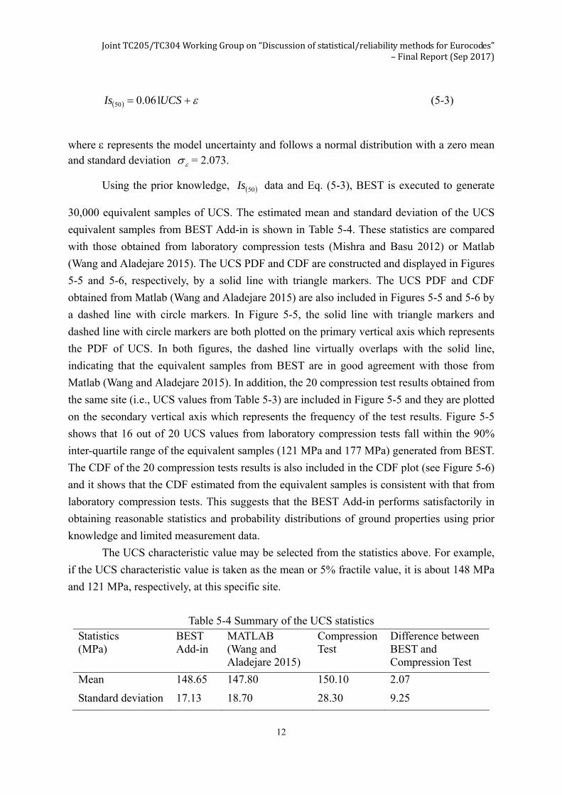
UCSIs 061.050 (5-3)

where represents the model uncertainty and follows a normal distribution with a zero mean and standard deviation = 2.073.

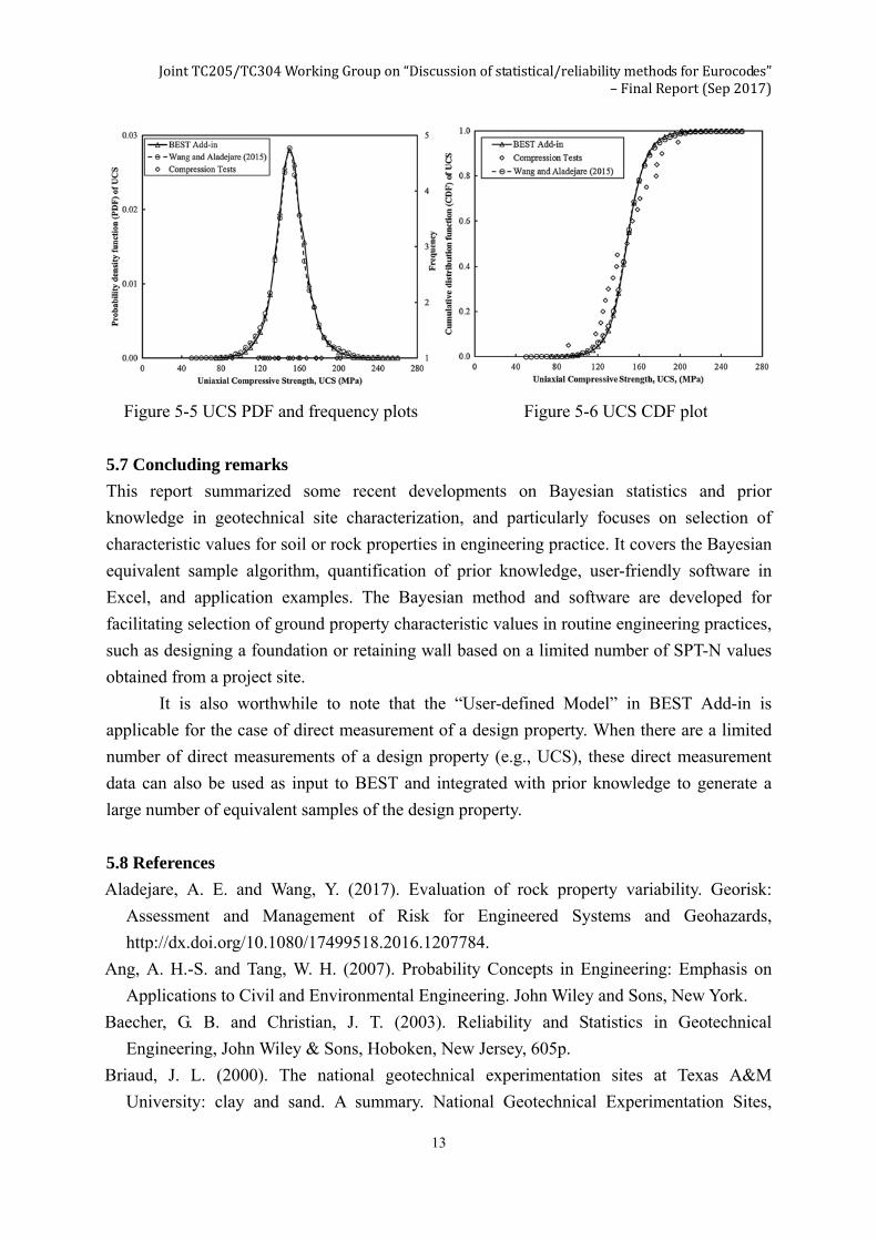
Using the prior knowledge, 50Is data and Eq. (5-3), BEST is executed to generate

30,000 equivalent samples of UCS. The estimated mean and standard deviation of the UCS

equivalent samples from BEST Add-in is shown in Table 5-4. These statistics are compared

with those obtained from laboratory compression tests (Mishra and Basu 2012) or Matlab

(Wang and Aladejare 2015). The UCS PDF and CDF are constructed and displayed in Figures

5-5 and 5-6, respectively, by a solid line with triangle markers. The UCS PDF and CDF

obtained from Matlab (Wang and Aladejare 2015) are also included in Figures 5-5 and 5-6 by

a dashed line with circle markers. In Figure 5-5, the solid line with triangle markers and

dashed line with circle markers are both plotted on the primary vertical axis which represents

the PDF of UCS. In both figures, the dashed line virtually overlaps with the solid line,

indicating that the equivalent samples from BEST are in good agreement with those from

Matlab (Wang and Aladejare 2015). In addition, the 20 compression test results obtained from

the same site (i.e., UCS values from Table 5-3) are included in Figure 5-5 and they are plotted

on the secondary vertical axis which represents the frequency of the test results. Figure 5-5

shows that 16 out of 20 UCS values from laboratory compression tests fall within the 90%

inter-quartile range of the equivalent samples (121 MPa and 177 MPa) generated from BEST.

The CDF of the 20 compression tests results is also included in the CDF plot (see Figure 5-6)

and it shows that the CDF estimated from the equivalent samples is consistent with that from

laboratory compression tests. This suggests that the BEST Add-in performs satisfactorily in

obtaining reasonable statistics and probability distributions of ground properties using prior

knowledge and limited measurement data.

The UCS characteristic value may be selected from the statistics above. For example,

if the UCS characteristic value is taken as the mean or 5% fractile value, it is about 148 MPa

and 121 MPa, respectively, at this specific site.

Table 5-4 Summary of the UCS statistics Statistics (MPa)

BEST Add-in

MATLAB (Wang and Aladejare 2015)

Compression Test

Difference between BEST and Compression Test

Mean 148.65 147.80 150.10 2.07

Standard deviation 17.13 18.70 28.30 9.25


13

Figure 5-5 UCS PDF and frequency plots Figure 5-6 UCS CDF plot

5.7 Concluding remarks

This report summarized some recent developments on Bayesian statistics and prior

knowledge in geotechnical site characterization, and particularly focuses on selection of

characteristic values for soil or rock properties in engineering practice. It covers the Bayesian

equivalent sample algorithm, quantification of prior knowledge, user-friendly software in

Excel, and application examples. The Bayesian method and software are developed for

facilitating selection of ground property characteristic values in routine engineering practices,

such as designing a foundation or retaining wall based on a limited number of SPT-N values

obtained from a project site.

It is also worthwhile to note that the “User-defined Model” in BEST Add-in is

applicable for the case of direct measurement of a design property. When there are a limited

number of direct measurements of a design property (e.g., UCS), these direct measurement

data can also be used as input to BEST and integrated with prior knowledge to generate a

large number of equivalent samples of the design property.

5.8 References

Aladejare, A. E. and Wang, Y. (2017). Evaluation of rock property variability. Georisk:

Assessment and Management of Risk for Engineered Systems and Geohazards,

http://dx.doi.org/10.1080/17499518.2016.1207784.

Ang, A. H.-S. and Tang, W. H. (2007). Probability Concepts in Engineering: Emphasis on

Applications to Civil and Environmental Engineering. John Wiley and Sons, New York.

Baecher, G. B. and Christian, J. T. (2003). Reliability and Statistics in Geotechnical

Engineering, John Wiley & Sons, Hoboken, New Jersey, 605p.

Briaud, J. L. (2000). The national geotechnical experimentation sites at Texas A&M

University: clay and sand. A summary. National Geotechnical Experimentation Sites,


14

ASCE GSP 93, 26–51.

Cao, Z. and Wang, Y. (2014). Bayesian model comparison and characterization of undrained

shear strength. Journal of Geotechnical & Geoenvironmental Engineering, 140(6),

04014018, 1-9.

Cao, Z., Wang, Y., and Li, D. (2016). Quantification of prior knowledge in geotechnical site

characterization. Engineering Geology, 203, 107-116.

CEN (2004) EN 1997-1:2004 Geotechnical Design – Part 1: General Rules.

Chau, K. T. and Wong, R. H. C. (1996) Uniaxial compressive strength and point load strength

of rocks, International Journal of Rock Mechanics & Mining Sciences, 33, 183–188.

Ching, J., Chen, J. R., Yeh, J. Y., and Phoon, K. K. (2012). Updating uncertainties in friction

angles of clean sands. Journal of Geotechnical and Geoenvironmental Engineering, 138(2),

217-229.

Clayton, C. R. I., Matthews. M. C., Simons, N. E. (1995). Site investigation. Blackwell

Science, Cambridge, Mass., USA.

Fenton, G. A., Naghibi, F., Dundas, D., Bathurst, R. J., and Griffiths, D. V. (2016).

Reliability-based geotechnical design in 2014 Canadian Highway Bridge Design Code.

Canadian Geotechnical Journal, 53(2), 236-251.

Kulhawy, F. H. and Mayne, P. W. (1990). Manual on Estimating Soil Properties for

Foundation Design, Report EL 6800, Electric Power Research Inst., Palo Alto, 306p.

Mayne, P. W., Christopher, B. R., and DeJong, J. (2002). Subsurface Investigations –

Geotechnical Site Characterization, No. FHWA NHI-01-031, Federal Highway

Administration, U. S. Department of Transportation, Washington D. C.

McLachlan, G. and Peel, D. (2000). Finite mixture models. New York, John Wiley & Sons.

Mishra, D. A. and Basu, A. (2012). Use of the block punch test to predict the compressive and

tensile strengths of rocks. International Journal of Rock Mechanics and Mining Sciences,

51, 119-27.

Orr, T. L. L. (2005). Design examples for the Eurocode 7 Workshop. Proceedings of the

international workshop on the evaluation of Eurocode 7, Trinity College, Dublin, 67–74.

Orr, T. L. L. (2017). Defining and selecting characteristic values of geotechnical parameters

for designs to Eurocode 7, Georisk: Assessment and Management of Risk for Engineered

Systems and Geohazards, DOI: 10.1080/17499518.2016.1235711.

Paikowsky, S. G., Birgisson, B., McVay, M., Nguyen, T., Kuo, C., Baecher, G., Ayyub, B.,

Stenersen, K., O’Malley, K., Chernauskas, L., and O’Neill, M. (2004). Load and resistance

factor design (LRFD) for deep foundations. NCHRP Report 507, Transportation Research

Board, Washington, DC.

Paikowsky, S. G., Canniff, M. C., Lesny, K., Kisse, A., Amatya, S., and Muganga, R. (2010).

LRFD design and construction of shallow foundations for highway bridge structures.

NCHRP Report 651, Transportation Research Board, Washington, DC.


15

Phoon K. K. (2017). Role of reliability calculations in geotechnical design, Georisk:

Assessment and Management of Risk for Engineered Systems and Geohazards, DOI:

10.1080/17499518.2016.1265653.

Phoon, K. K. and Kulhawy, F. H. (1999a). Characterization of geotechnical variability.


Phoon, K. K. and Kulhawy, F. H. (1999b). Evaluation of geotechnical property variability.


Phoon, K. K., Kulhawy, F. H., and Grigoriu, M. D. (2003a). Development of a

reliability-based design framework for transmission line structure foundations. Journal of

Geotechnical and Geoenvironmental Engineering, 129(9), 798-806.

Phoon, K. K., Kulhawy, F. H., and Grigoriu, M. D. (2003b). Multiple resistance factor design

(MRFD) for shallow transmission line structure foundations. Journal of Geotechnical and

Geoenvironmental Engineering, 129(9), 807-818.

Phoon, K. K., Retief, J. V., Ching, J., Dithinde, M., Schweckendiek, T., Wang, Y., and Zhang

L. M. (2016). Some observations on ISO2394: 2015 Annex D (Reliability of Geotechnical

Structures). Structural Safety, 62, 24-33.

Robert, C. and Casella, G. (2004). Monte Carlo Statistical Methods. Springer.

Schneider, H. R. and Schneider, M. A. (2013). Dealing with uncertainties in EC7 with

emphasis on determination of characteristic soil properties. Modern Geotechnical Design

Codes of Practice, P. Arnold et al. (Eds.), ISO Press, 87-101.

Trautmann, C.H. and Kulhawy, F.H. (1983). Data sources for engineering geologic studies.

Bull. Assn. Eng. Geologists, 20(4), 439-454.

Vick, S. G. (2002). Degrees of Belief: Subjective Probability and Engineering Judgment.

ASCE Press, Reston, Virginia.

Wang, Y., Akeju, O. V., and Cao, Z. (2016b). Bayesian Equivalent Sample Toolkit (BEST): an

Excel VBA program for probabilistic characterisation of geotechnical properties from

limited observation data. Georisk, 10(4), 251-268.

Wang, Y. and Aladejare, A. E. (2015). Selection of site-specific regression model for

characterization of uniaxial compressive strength of rock. International Journal of Rock

Mechanics & Mining Sciences, 75, 73-81.

Wang, Y. and Cao, Z. (2013). Probabilistic characterization of Young's modulus of soil using

equivalent samples. Engineering Geology, 159, 106-118.

Wang, Y., Cao, Z., and Li, D. (2016a). Bayesian perspective on geotechnical variability and

site characterization. Engineering Geology, 203, 117-125.

Wang, Y., Zhao, T., and Cao, Z. (2015). Site-specific probability distribution of geotechnical

properties. Computers and Geotechnics, 70, 159-168.


16

Discussions and Replies

During the preparation of this report, many valuable and insightful comments and

suggestions have been gratefully received. Some of them have been incorporated in this final

draft report, including those made by Marcos Arroya, Zijun Cao and Trevor Orr, and hence,

they do not appear in this section. The other comments and suggestions are listed below by

the date they were received.

Discussion by Tim Länsivaara (Tampere University of Technology, Finland)

I think this is a very important issue and it would be great to have some progress in the form

on guidelines in the determination of characteristic values. I think it would be good to first

also discuss what is the definition of a characteristic value. Personally I don't think that the

definition in Eurocodes as a 5% fractile value is a very good one.

Reply by Yu Wang (City University of Hong Kong, Hong Kong)

This draft final report contains a section (i.e., Section 5.2) on the definition of characteristic

value. However, the definition of characteristic value for ground properties itself might be an

intriguing issue, and detailed discussion on this issue is beyond the scope of this report,

which focus on using Bayesian statistics and prior knowledge to facilitate the proper selection

of characteristic value for a given definition of characteristic value. Detailed discussion on

definition of characteristic value in EC7 is referred to Schneider and Schneider (2013) and

Orr (2017).

Discussion by KK Phoon (National University of Singapore, Singapore)

Some observations on characteristic value

EN 1997−1:2004, 2.4.5.2(2) recommends that the “characteristic value of a geotechnical

parameter shall be selected as a cautious estimate of the value affecting the occurrence of the

limit state.” Much attention has been focused on how to obtain a “cautious estimate”. For

example, EN 1997−1:2004, 2.4.5.2(11) notes that “If statistical methods are used, the

characteristic value should be derived such that the calculated probability of a worse value

governing the occurrence of the limit state under consideration is not greater than 5%.” A

note to this clause clarifies that “In this respect, a cautious estimate of the mean value is a

selection of the mean value of the limited set of geotechnical parameter values, with a

confidence level of 95%; where local failure is concerned, a cautious estimate of the low

value is a 5% fractile.” Less attention is focused on the “value affecting the occurrence of

the limit state”.


17

In my opinion, the general statement describing the characteristic value “as a cautious

estimate of the value affecting the occurrence of the limit state” is sensible.

However, there is an under-stated difficulty in making this statement sufficiently concrete for

codification.

We acknowledge the critical role of engineering judgment. Sensibility and reality checks on

all design aspects are clearly dependent on informed judgment. This discussion focuses only

on those numerical aspects that probabilistic methods can add value to the estimation of the

characteristic value.

In my opinion, it is crucial to examine the following 2 elements: (1) “value affecting the

occurrence of the limit state” and (2) “cautious estimate” separately.

Value affecting the occurrence of the limit state

One can visualize the first element “value affecting the occurrence of the limit state” more

clearly by assuming there is no uncertainty. In other words, we only look at one realization

of a random field. It can be spatially heterogeneous or even spatially homogeneous in

horizontal and/or vertical directions when the scales of fluctuation are large in those

directions. We can assume we have sufficient direct measurements to safely ignore

transformation and statistical uncertainties. Under this ideal deterministic condition, the first

element is a question in mechanics.

Consider a bored pile as a concrete example. One can argue that the side resistance depends

on the average strength in each layer supporting the pile. The tip resistance can conceivably

be seen as depending on the average strength below one diameter of the tip. The mobilized

strength “value” is related to the average over an influential volume of soil.

Consider a slope stability problem as a second example. For a homogeneous slope, the

mobilized strength along the critical slip surface can be viewed as another average of a

homogeneous soil mass. For a heterogeneous slope, the same argument applies, but an

intriguing difficulty arises in this instance. If an engineer analyses this slope with

characteristic values in each layer estimated from borehole/field test data (however they are

selected), the relative magnitude of the characteristic values can affect the location of the

critical slip surface emerging from a mechanical analysis, say limit equilibrium or finite

element analysis. This slip surface may or may not be the same as the one emerging from a

finite element analysis adopting the strength reduction approach.


18

The central difficulty is that the “occurrence of the limit state” is an output of a mechanical

analysis; it is not linked to borehole/field test data (input) in a straightforward way although

an experienced engineer could make an informed guess. An inexperienced engineer may

judge incorrectly without guidance from a mechanical analysis.

Cautious estimate

The second element “cautious estimate” only arises in the presence of uncertainty. Spatial

variability and a range of uncertainties (transformation, statistical, etc.) allow a range of

possible values and possible scenarios to exist, because measured data are too limited to

restrict a property to a single value and a profile to a single scenario. However the “value

affecting the occurrence of the limit state” is defined, it is clear that it will also take a range of

values in the presence of uncertainty, i.e. it is a random variable.

The key point is that this random variable is not necessarily the same as the random variable

describing a soil property at a “point”.

If one accepts the average along the pile shaft as the “value affecting the occurrence of the

limit state”, then the relevant random variable is the spatial average over the length of the

shaft. If one further accepts that a customarily 95% confidence level is sufficient, that is

select a threshold value so that the actual value will exceed this threshold value with 95%

probability, then this definition is partially consistent with the statement “a cautious estimate

of the mean value is a selection of the mean value of the limited set of geotechnical parameter

values, with a confidence level of 95%”. This definition is also consistent with a 5%

quantile (or fractile) of the spatial average (in the reliability literature).

The key difference is that the spatial average is a function of the length of the shaft while this

length effect is not explicitly stated with reference to the “mean” in EN 1997−1:2004,

2.4.5.2(11). It goes without saying that the spatial average and the mean are affected by

statistical uncertainty and this is related to the number of measurements.

For the statement “where local failure is concerned, a cautious estimate of the low value is a

5% fractile”, it is somewhat ambiguous in probabilistic terms, but my interpretation is that

EN 1997−1:2004, 2.4.5.2(11) is referring to 5% quantile (or fractile) of the soil property at a

“point”.

ISO2394:2015 (Annex D) Section D.5.5 discusses the need to clarify the mechanical and

probabilistic aspects of the characteristic value (refer to excerpt below).


19

Closing thoughts for discussion

1. Statistical analysis of site information typically produces the statistics (mean,

coefficient of variation) for a soil property at a “point”. The “point” random variable

described by these statistics is not the same as the “mobilized” random variable

“affecting the occurrence of the limit state”. To be specific, if the limit state involves

bearing capacity, the “mobilized” random variable appearing in the bearing capacity

equation is not the same as the “point” random variable. In other words, the

“mobilized” random variable is the one relevant to the resistance/response calculation

model.

2. The “occurrence of the limit state” is an output of a mechanical analysis. It is not

straightforward to define this “mobilized” random variable from input soil data alone.

This definition can depend on the limit state. EN 1997−1:2004, 2.4.5.2(11) already

noted that the distinction between non- local and local failures. In my opinion, more

research is needed. The best one can hope for is to define a “mobilized” random

variable so that it approximates the probabilistic solution from a mechanical analysis

(say random finite element analysis) with reasonable accuracy.

3. In my opinion, there are merits to replace term “mean” stated in EN 1997−1:2004,

2.4.5.2(11) by the “spatial average”:

a. “Mean” is a statistics for a set of measurements. It does not focus the

attention of the engineer on the limit state. The spatial average depends on

the averaging domain (line/surface/volume) where the limit state is

expected to take place.

b. One concrete improvement is that the characteristic value will depend on

the size of the averaging domain (e.g. length of the pile shaft) if we refer to

“spatial average”.

c. The uncertainty in the mean only depends on the number of measurements

(statistical uncertainty). Spatial average can include other sources of

uncertainties, including statistical uncertainty (see #7 below). In this sense,

it is a more general and more physically meaningful concept.

4. Even the classical spatial average (Vanmarcke 1977) is an approximate solution,

because the average along the critical slip path/surface is not the same as the average

along a fixed prescribed path/surface. The former path/surface is partially affected by

the distribution of “weak zones” in a spatially varying soil mass, which changes from

realization to realization. The literature says that the classical spatial average is

reasonable if the scale of fluctuation does not take a “critical” value (Ching & Phoon

2013; Ching et al. 2014, 2016a). Hence, the spatial average can be retained as a

first-order approximation of the mobilized random variable for the time being. The


20

5% fractile of this spatial average can be used as a more concrete definition of the

characteristic value for the time being, when it is suitably qualified.

5. For limit states not governed by spatial averages, e.g. local failure, seepage, etc.,

more research is needed to clarify if the “mobilized” and “point” random variables are

the same.

6. From the perspective of a “mobilized” random variable, the terms “confidence level

of 95%” and “5% fractile” are the same. I would recommend harmonizing these terms

in in EN 1997−1:2004, 2.4.5.2(11) to “5% fractile of the mobilized random variable”.

The mobilized random variable can be approximated by the spatial average or other

random quantities depending on the occurrence of the limit state.

7. The coefficient of variation of the mobilized random variable is affected by statistical

uncertainty (due to limited measurements), spatial variability (due to spatial extent of

limit state), measurement error (due to measurement), and transformation uncertainty

(due to conversion from measurements to desired properties). Statistical uncertainty is

already covered in EN 1997−1:2004, 2.4.5.2, but extensive research has shown that

other sources are present (Ching et al. 2016b; Phoon et al. 2016).

References

1. Ching, J. & Phoon, K. K. (2013b). Probability distribution for mobilized shear strengths of

spatially variable soils under uniform stress states. Georisk, 7(3), 209-224.

2. Ching, J., Phoon, K. K. & Kao, P. H. (2014). Mean and variance of the mobilized shear

strengths for spatially variable soils under uniform stress states. ASCE Journal of

Engineering Mechanics, 140(3), 487-501

3. Ching, J., Lee, S. W. & Phoon, K. K. (2016a). Undrained strength for a 3D spatially

variable clay column subjected to compression or shear. Probabilistic Engineering

Mechanics, 45, 127–139.

4. Ching, J. Y., Li, D. Q. & Phoon, K. K. (2016b). Statistical characterization of multivariate

geotechnical data, Chapter 4, Reliability of Geotechnical Structures in ISO2394, Eds.

K. K. Phoon & J. V. Retief, CRC Press/Balkema, 89-126.

5. Phoon, K. K., Prakoso, W. A., Wang, Y., Ching, J. Y. (2016). Uncertainty representation of

geotechnical design parameters, Chapter 3, Reliability of Geotechnical Structures in

ISO2394, Eds. K. K. Phoon & J. V. Retief, CRC Press/Balkema, 2016, 49-87.

6. Vanmarcke, E. H. (1977). “Probabilistic modeling of soil profiles”, Journal of Geotechnical

Engineering Division, ASCE, 103(GT11), 1227 – 1246.

Excerpt from ISO2394:2015 General principles on reliability for structures, Annex D

Reliability of Geotechnical Structures


21

D.5.5 Characteristic value

The concept of a “characteristic value” is intrinsically linked to semi-probabilistic formats,

particularly the partial factor approach. In this approach, using the ultimate limit state as an

example, a “characteristic value” for a soil parameter (e.g., undrained shear strength), is

divided by a strength partial factor to produce a “design” value and the geotechnical

capacity based on this design value should be larger than the design load (characteristic load

multiplied by a load factor).

The soil parameter must be defined such that it is relevant to the limit state equation. For

example, if a single undrained shear strength parameter appears in a slope stability equation,

then the relevant physical definition is the spatial average along the most critical failure path.

It is neither the undrained shear strength at a point in the soil mass nor a spatial average along

a prescribed line in the soil mass. The emphasis in the geotechnical literature is on clarifying

this physical aspect of the characteristic value, which is justifiably so.

It is necessary to make clear the physical meaning of the characteristic soil parameter before

the uncertainty aspect could be rationally considered. For illustration, the characteristic

undrained shear strength for the shaft friction of a pile is the spatial average along the length

of the pile, while the characteristic undrained shear strength for the end bearing of a pile is

the spatial average within a bulb of soil below the pile tip. When reliability analysis is carried

out, the performance function will contain two random variables following two distinct

probability distributions for these spatial averages.

When semi-probabilistic design is carried out, it would be necessary to select a single value

characteristic of each probability distribution. This value may refer to the mean or to the

lower 5% quantile. The statistical estimation of these characteristic values is subject to the

same statistical uncertainties underlying the probability distributions appearing in reliability

analysis. Clearly, this statistical aspect of the characteristic value is distinctive from the

physical aspect of the characteristic value.

In principle, partial factors can be calibrated to achieve a prescribed target reliability index

for any statistical definition of the characteristic value. In practice, it is known that a partial

factor calibrated for the mean value could change significantly if the COV of the input

random variable changes. This limitation is less severe for a partial factor calibrated using say

the lower 5%-quantile. Hence, if the COV of an input random variable varies over a wide

range within the scope of design scenarios covered in a design code and if there is a practical

need to simplify presentation of a partial factor as a single number rather than as a function of

COV, the lower 5% quantile definition is preferred (except in the case considering non-linear


22

responses where special considerations must be made). It is useful to reiterate that the key

function of a RBD code is to achieve a prescribed target reliability index (typically a function

of limit state and importance of structure) over a range of commonly encountered design

scenarios and not for a specific design scenario. The statistical definition of the characteristic

value should be viewed within this broader context of what a RBD code intends to achieve,

rather than adherence to past practice or a component separate from reliability calibration.

In other words, the ensuing design is produced by design values, which is the product of

partial/resistance factors with characteristic values, not merely characteristic values alone.

There are practical concerns regarding: (1) estimation of quantiles reliably from limited data

and (2) quantiles falling below known lower bounds (e.g. residual friction angle) due to

inappropriate choice of unbounded probability distribution functions. However, both

concerns do not merely affect the characteristic value but fundamentally affect the reliability

analyses underlying code calibration as well.


Although the definition of ground property characteristic values is clearly given in the

Eurocodes (both the head code and EC7), it seems that there are some practical difficulty in

implementing this definition in geotechnical practice, due to, for example, site-specific nature

of ground properties, generally small sample size of site-specific data, usage of engineering

experience and judgment (e.g., previous data from similar project or site conditions). In

addition, the characteristic values in EC7 are linked with the output of a design calculation,

i.e., “a question in mechanics” as pointed out in the discussion above. This indeed is a

dilemma of “Which came first: the chicken or the egg?” because the characteristic values are

supposed to be defined first for the subsequent design calculation.

A possible way out of this dilemma is to revise the definition of characteristic values in such

a way that it does not involve the design calculation (or the “mechanics” of a design) when

selecting the characteristic values. In other words, the characteristic value may be defined to

reflect only the existing information on the site, including site-specific test data and

pre-existing engineering experience and judgment as shown in this report.

The advantage of such a definition is that it allows different practitioners to arrive at the same

characteristic value from a given (i.e., the same) set of site-specific test data and pre-existing

engineering experience and judgment, even for different design problems (e.g., foundations,

slope stability). Then, based on different design problems, different influence zones are

identified, and the characteristic values within the corresponding influence zones are used in

the design calculations. For example, the influence zone for a shallow foundation is about one

diameter of the foundation width below the foundation, and that for the side resistance of a


23

pile is the length of the pile. This is consistent with the conventional (or deterministic)

practice in geotechnical engineering.

The disadvantages of such a definition is that many sophisticated and important issues raised

in the discussion above will NOT be considered in the definition of characteristic value, such

as the “mobilized” random variable for different design problems (e.g., foundations, slope

stability) and spatial averaging along a fixed surface vs an unknown surface. All these

important issues involve the “mechanics” of the design problem under consideration, and

they should be properly considered by other means in design codes, such as partial factors.

Calibration of the partial factors always involves the “mechanics” of the design problem

under consideration, and it is problem specific. It might be logical and convenient to remove

all the “mechanics” related issues from the definition of characteristic values and incorporate

them systematically during the calibration of partial factors.

It is also worth noting that, as pointed out in the discussion above, “The concept of a

“characteristic value” is intrinsically linked to semi-probabilistic formats, particularly the

partial factor approach.” If using a single characteristic value in semi-probabilistic formats is

NOT able to properly reflect the “mechanics” of the design problem under consideration (e.g.,

the occurrence of different failure modes for different characteristic values adopted), direct

probability-based design methods may be used for these sophisticated design problems.

Detailed discussion on the direct probability-based design methods in geotechnical

engineering is given by Wang et al. (2016).

Reference:

Wang, Y., Schweckendiek, T., Gong, W., Zhao, T., and Phoon, K. K. (2016). Direct

probability-based design methods, Chapter 7 in Reliability of Geotechnical Structures In

ISO2394, Edited by K. K. Phoon, J. V. Retief, Pages 193–226, DOI:

10.1201/9781315364179-8.

Discussion by Jianye Ching (National Taiwan University, Taiwan)

I would like to share with all of you our (KK & myself) recent findings regarding

characteristic value. The findings below have been confirmed by numerical evidences

obtained from random field finite element.

1. The mechanism for shear strength is that the "effective" shear strength should be the

average along the critical slip surface. Here, the spatial averaging takes effect. This means

that the effective shear strength has a variance less than the inherent variance. However, the


24

difficult part is that the critical slip surface is unknown. Therefore, the spatial averaging

cannot be taken over a "prescribed" soil volume. Because the critical slip surface may seek

for the weak zone, the effective shear strength has a mean value less than the inherent mean.

2. The mechanism for deformation is quite different. We just found that the effective Young's

modulus can be represented as a spatial average over a "prescribed" soil volume. However,

the degree of mobilization is not uniform over the entire soil mass. This is intuitive, e.g., the

soil volume right below a footing is more mobilized than another soil volume remote to the

footing.

I think characteristic value can be defined as the cautious estimate for the mean value of the

effective shear strength or effective Young's modulus.

We have proposed probabilistic models to characterize the effective shear strength &

effective Young's modulus. These models are able to predict the probability distributions for

the effective shear strength & effective Young's modulus. They depend on the inherent mean,

inherent variance, scales of fluctuation, and problem geometry.


The comments and issues raised by Jianye are of great importance, and they echo and

supplement the comments raised by KK. Please refer to the reply to KK’s discussion above

for a detailed reply.

Discussion by Brian Simpson (Arup, UK)

I found this report very interesting. I do think that Bayesian methods could be very helpful

in deriving characteristic values of parameters. Thanks to Yu Wang.

I have a concern, however, about the definition of characteristic value, as understood in EC7.

In the report, it seems to be treated as a 5% fractile of test results, which is not the intention

of EC7. The author might want to comment further on this.

The basic definition given in EC7 is that the characteristic value is a “a cautious estimate of

the value affecting the occurrence of the limit state” (2.4.5.2(2)). The paragraphs that

follow this are important, including (7):

The zone of ground governing the behaviour of a geotechnical structure at a limit state

is usually much larger than a test sample or the zone of ground affected in an in situ

test. Consequently the value of the governing parameter is often the mean of a range


25

of values covering a large surface or volume of the ground. The characteristic value

should be a cautious estimate of this mean value.

And (9):

When selecting the zone of ground governing the behaviour of a geotechnical

structure at a limit state, it should be considered that this limit state may depend on

the behaviour of the supported structure. For instance, when considering a bearing

resistance ultimate limit state for a building resting on several footings, the governing

parameter should be the mean strength over each individual zone of ground under a

footing, if the building is unable to resist a local failure. If, however, the building is

stiff and strong enough, the governing parameter should be the mean of these mean

values over the entire zone or part of the zone of ground under the building.

Paragraph (11) says:

If statistical methods are used, the characteristic value should be derived such that the

calculated probability of a worse value governing the occurrence of the limit state

under consideration is not greater than 5%.

And the note attached to that is important:

In this respect, a cautious estimate of the mean value is a selection of the mean value

of the limited set of geotechnical parameter values, with a confidence level of 95%;

where local failure is concerned, a cautious estimate of the low value is a 5% fractile.

It should be clear from this that the characteristic value required by EC7 is not a 5% fractile

of test results, but rather there is a 5% probability that a worse value could be representative

of the whole body or surface of soil that governs the occurrence of the limit state.

Schneider (1997) suggested that given at least 10 test results, the 5% probability value for the

mean of the population lies about half a standard deviation from the mean of the test results.

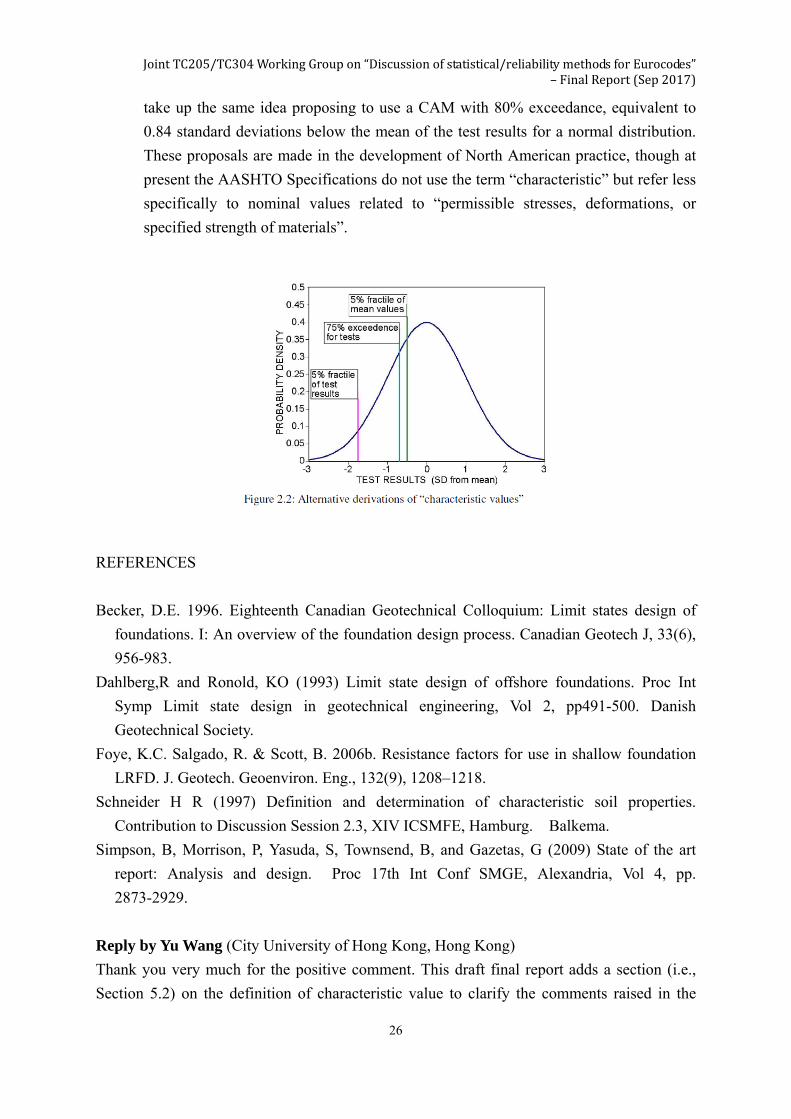
His ideas have been developed further since then. The following figure, taken from

Simpson et al (2009) shows that this is much nearer the mean than the 5% fractile of the test

results (obviously). The following paragraph, taken from the same paper, suggests that this

may not be very different from North American practice:

A similar proposal was made by Dahlberg and Ronold (1993) for design of offshore

foundations and recommended by Becker (1996) for more general use. This involves

the use of a “conservatively assessed mean” (CAM) as the characteristic value, also

about 0.5 standard deviations from the mean of the test results. These authors state

that for a normal distribution 75% of the measured values would be expected to

exceed this value. (More accurately, this requires an offset of 0.69 standard deviations

from the mean, for a normal distribution, as shown in Figure 2.2). Foye et al (2006b)


26

take up the same idea proposing to use a CAM with 80% exceedance, equivalent to

0.84 standard deviations below the mean of the test results for a normal distribution.

These proposals are made in the development of North American practice, though at

present the AASHTO Specifications do not use the term “characteristic” but refer less

specifically to nominal values related to “permissible stresses, deformations, or

specified strength of materials”.

REFERENCES

Becker, D.E. 1996. Eighteenth Canadian Geotechnical Colloquium: Limit states design of

foundations. I: An overview of the foundation design process. Canadian Geotech J, 33(6),

956-983.

Dahlberg,R and Ronold, KO (1993) Limit state design of offshore foundations. Proc Int

Symp Limit state design in geotechnical engineering, Vol 2, pp491-500. Danish

Geotechnical Society.

Foye, K.C. Salgado, R. & Scott, B. 2006b. Resistance factors for use in shallow foundation

LRFD. J. Geotech. Geoenviron. Eng., 132(9), 1208–1218.

Schneider H R (1997) Definition and determination of characteristic soil properties.

Contribution to Discussion Session 2.3, XIV ICSMFE, Hamburg. Balkema.

Simpson, B, Morrison, P, Yasuda, S, Townsend, B, and Gazetas, G (2009) State of the art

report: Analysis and design. Proc 17th Int Conf SMGE, Alexandria, Vol 4, pp.

2873-2929.


Thank you very much for the positive comment. This draft final report adds a section (i.e.,

Section 5.2) on the definition of characteristic value to clarify the comments raised in the


27

discussion. However, the definition of characteristic value for ground properties itself might

be an intriguing issue, and detailed discussion on this issue is beyond the scope of this report,

which focus on using Bayesian statistics and prior knowledge to facilitate the proper selection

of characteristic value for a given definition of characteristic value. Detailed discussion on

definition of characteristic value in EC7 is referred to Schneider and Schneider (2013) and

Orr (2017). The illustrative examples in this report have also been revised to highlight that,

when the characteristic value is defined in different way, different numerical values will be

obtained accordingly.

chapter 5 - characteristic values from bayesian statistics...

Documents