1

CHAPTER 5

CAPACITORS

5.1 Introduction

A capacitor consists of two metal plates separated by a nonconducting medium (known

as the dielectric medium or simply the dielectric, or by a vacuum. It is represented by

the electrical symbol

.

Capacitors of one sort or another are included in almost any electronic device.

Physically, there is a vast variety of shapes, sizes and construction, depending upon their

particular application. This chapter, however, is not primarily concerned with real,

practical capacitors and how they are made and what they are used for, although a brief

section at the end of the chapter will discuss this. In addition to their practical uses in

electronic circuits, capacitors are very useful to professors for torturing students during

exams, and, more importantly, for helping students to understand the concepts of and the

relationships between electric fields E and D, potential difference, permittivity, energy,

and so on. The capacitors in this chapter are, for the most part, imaginary academic

concepts useful largely for pedagogical purposes. Need the electronics technician or

electronics engineer spend time on these academic capacitors, apparently so far removed

from the real devices to be found in electronic equipment? The answer is surely and

decidedly yes – more than anyone else, the practical technician or engineer must

thoroughly understand the basic concepts of electricity before even starting with real

electronic devices.

If a potential difference is maintained across the two plates of a capacitor (for example,

by connecting the plates across the poles of a battery) a charge +Q will be stored on one

plate and −Q on the other. The ratio of the charge stored on the plates to the potential

difference V across them is called the capacitance C of the capacitor. Thus:

.CVQ = 5.1.1

If, when the potential difference is one volt, the charge stored is one coulomb, the

capacitance is one farad, F. Thus, a farad is a coulomb per volt. It should be mentioned

here that, in practical terms, a farad is a very large unit of capacitance, and most

capacitors have capacitances of the order of microfarads, µF.

The dimensions of capacitance are .QTLMQTML

Q 2221

122

−−

−−=

2

It might be remarked that, in older books, a capacitor was called a “condenser”, and its capacitance was

called its “capacity”. Thus what we would now call the “capacitance of a capacitor” was formerly called

the “capacity of a condenser”.

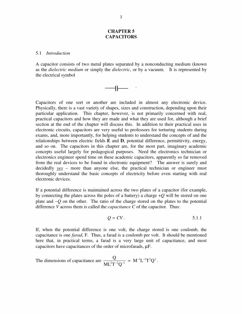
In the highly idealized capacitors of this chapter, the linear dimensions of the plates

(length and breadth, or diameter) are supposed to be very much larger than the separation

between them. This in fact is nearly always the case in real capacitors, too, though

perhaps not necessarily for the same reason. In real capacitors, the distance between the

plates is small so that the capacitance is as large as possible. In the imaginary capacitors

of this chapter, I want the separation to be small so that the electric field between the

plates is uniform. Thus the capacitors I shall be discussing are mostly like figure V.1,

where I have indicated, in blue, the electric field between the plates:

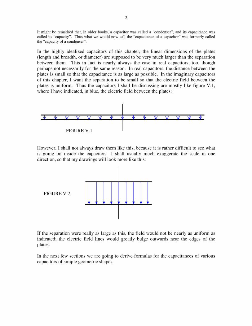
However, I shall not always draw them like this, because it is rather difficult to see what

is going on inside the capacitor. I shall usually much exaggerate the scale in one

direction, so that my drawings will look more like this:

If the separation were really as large as this, the field would not be nearly as uniform as

indicated; the electric field lines would greatly bulge outwards near the edges of the

plates.

In the next few sections we are going to derive formulas for the capacitances of various

capacitors of simple geometric shapes.

FIGURE V.1

FIGURE V.2

3

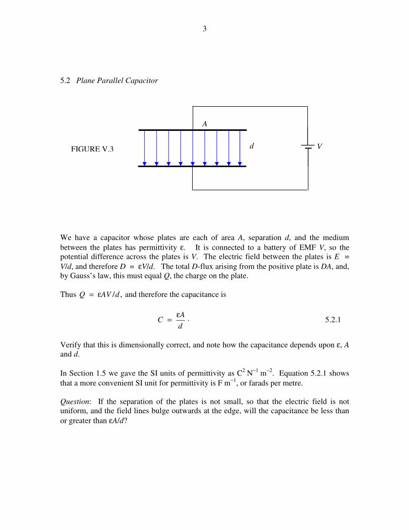
5.2 Plane Parallel Capacitor

We have a capacitor whose plates are each of area A, separation d, and the medium

between the plates has permittivity ε. It is connected to a battery of EMF V, so the

potential difference across the plates is V. The electric field between the plates is E =

V/d, and therefore D = εV/d. The total D-flux arising from the positive plate is DA, and,

by Gauss’s law, this must equal Q, the charge on the plate.

Thus ,/dAVQ ε= and therefore the capacitance is

.d

AC

ε= 5.2.1

Verify that this is dimensionally correct, and note how the capacitance depends upon ε, A

and d.

In Section 1.5 we gave the SI units of permittivity as C2

N−1

m−2

. Equation 5.2.1 shows

that a more convenient SI unit for permittivity is F m−1

, or farads per metre.

Question: If the separation of the plates is not small, so that the electric field is not

uniform, and the field lines bulge outwards at the edge, will the capacitance be less than

or greater than εA/d?

FIGURE V.3 V

A

d

4

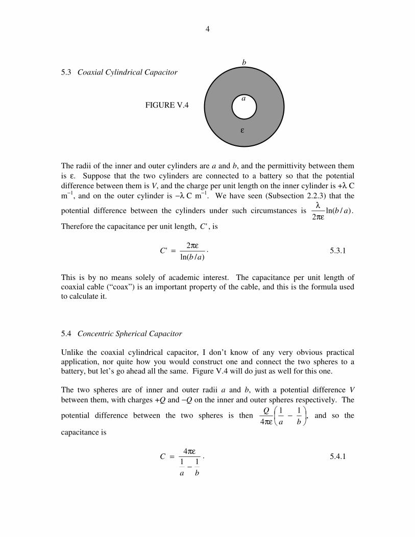
5.3 Coaxial Cylindrical Capacitor

The radii of the inner and outer cylinders are a and b, and the permittivity between them

is ε. Suppose that the two cylinders are connected to a battery so that the potential

difference between them is V, and the charge per unit length on the inner cylinder is +λ C

m−1

, and on the outer cylinder is −λ C m−1

. We have seen (Subsection 2.2.3) that the

potential difference between the cylinders under such circumstances is .)/ln(2

abπε

λ

Therefore the capacitance per unit length, 'C , is

.)/ln(

2'

abC

πε= 5.3.1

This is by no means solely of academic interest. The capacitance per unit length of

coaxial cable (“coax”) is an important property of the cable, and this is the formula used

to calculate it.

5.4 Concentric Spherical Capacitor

Unlike the coaxial cylindrical capacitor, I don’t know of any very obvious practical

application, nor quite how you would construct one and connect the two spheres to a

battery, but let’s go ahead all the same. Figure V.4 will do just as well for this one.

The two spheres are of inner and outer radii a and b, with a potential difference V

between them, with charges +Q and −Q on the inner and outer spheres respectively. The

potential difference between the two spheres is then ,11

4

−

πε ba

Q and so the

capacitance is

.11

4

ba

C

−

πε= 5.4.1

a

ε

b

FIGURE V.4

5

If ,∞→b we obtain for the capacitance of an isolated sphere of radius a:

.4 aC πε= 5.4.2

Exercise: Calculate the capacitance of planet Earth, of radius 6.371 × 103 km, suspended

in free space. I make it 709 µF - which may be a bit smaller than you were expecting.

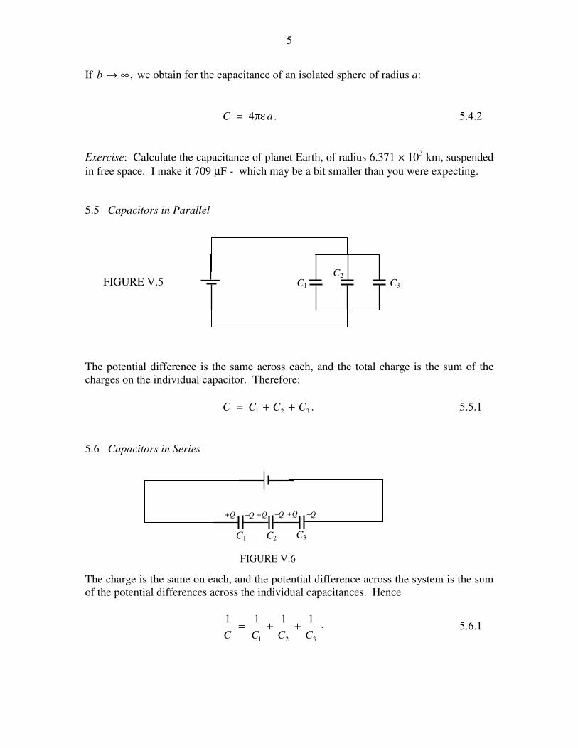
5.5 Capacitors in Parallel

The potential difference is the same across each, and the total charge is the sum of the

charges on the individual capacitor. Therefore:

.321 CCCC ++= 5.5.1

5.6 Capacitors in Series

The charge is the same on each, and the potential difference across the system is the sum

of the potential differences across the individual capacitances. Hence

.1111

321 CCCC++= 5.6.1

C1 C3

C2

FIGURE V.5

C1 C2 C3

+Q +Q +Q −Q −Q −Q

FIGURE V.6

6

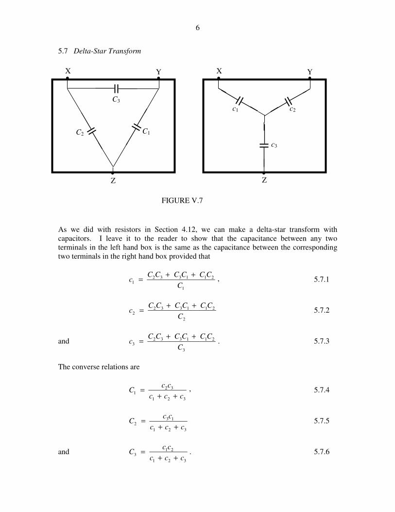
5.7 Delta-Star Transform

As we did with resistors in Section 4.12, we can make a delta-star transform with

capacitors. I leave it to the reader to show that the capacitance between any two

terminals in the left hand box is the same as the capacitance between the corresponding

two terminals in the right hand box provided that

,1

2113321

C

CCCCCCc

++= 5.7.1

2

2113322

C

CCCCCCc

++= 5.7.2

and .3

2113323

C

CCCCCCc

++= 5.7.3

The converse relations are

,

321

321

ccc

ccC

++= 5.7.4

321

132

ccc

ccC

++= 5.7.5

and .321

213

ccc

ccC

++= 5.7.6

Z

X

Z

• •

•

Y

c1 c2

c3

FIGURE V.7

X

C1

C3

C2

• •

•

Y

7

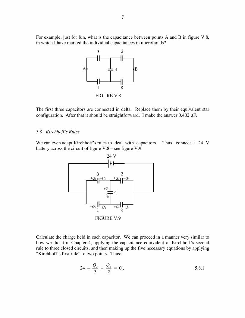
For example, just for fun, what is the capacitance between points A and B in figure V.8,

in which I have marked the individual capacitances in microfarads?

The first three capacitors are connected in delta. Replace them by their equivalent star

configuration. After that it should be straightforward. I make the answer 0.402 µF.

5.8 Kirchhoff’s Rules

We can even adapt Kirchhoff’s rules to deal with capacitors. Thus, connect a 24 V

battery across the circuit of figure V.8 – see figure V.9

Calculate the charge held in each capacitor. We can proceed in a manner very similar to

how we did it in Chapter 4, applying the capacitance equivalent of Kirchhoff’s second

rule to three closed circuits, and then making up the five necessary equations by applying

“Kirchhoff’s first rule” to two points. Thus:

,023

24 32 =−−QQ

5.8.1

•B A•

FIGURE V.8

3 2

4

1 8

FIGURE V.9

3 2

4

1 8

24 V

+Q1

+Q2 −Q2

+Q3 −Q3

+Q4 −Q4

+Q5

−Q5

−Q1

8

,08

24 42 =−−

QQ 5.8.2

,043

52

1 =+−Q

QQ

5.8.3

,531 QQQ += 5.8.4

and .524 QQQ += 5.8.5

I make the solutions

.C91.20,C92.39,C44.20,C01.19,C35.41 54321 µ+=µ+=µ+=µ+=µ+= QQQQQ

5.9 Problem for a Rainy Day

Another problem to while away a rainy Sunday afternoon would be to replace each of the

resistors in the cube of subsection 4.14.1 with capacitors each of capacitance c. What is

the total capacitance across opposite corners of the cube? I would start by supposing that

the cube holds a net charge of 6Q, and I would then ask myself what is the charge held in

each of the individual capacitors. And I would then follow the potential drop from one

corner of the cube to the opposite corner. I make the answer for the effective capacitance

of the entire cube 1.2c.

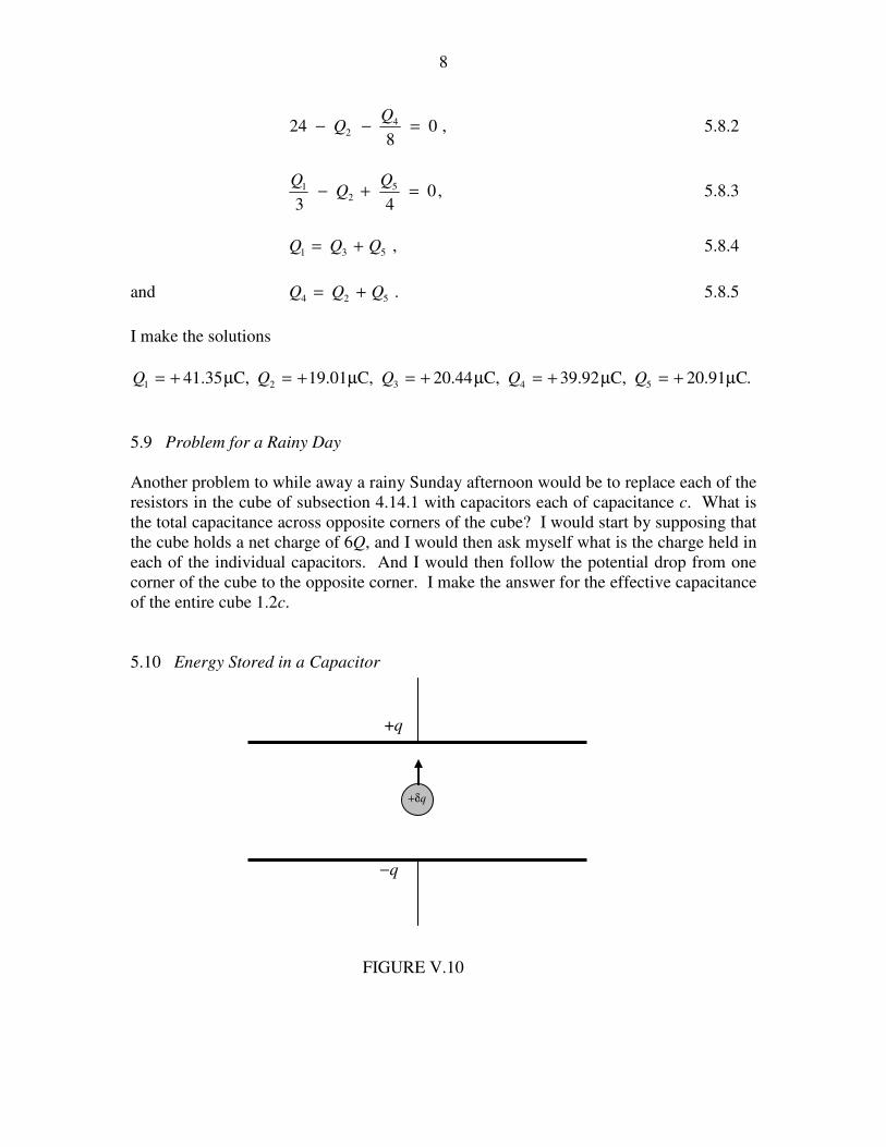
5.10 Energy Stored in a Capacitor

+q

+δq

−q

FIGURE V.10

9

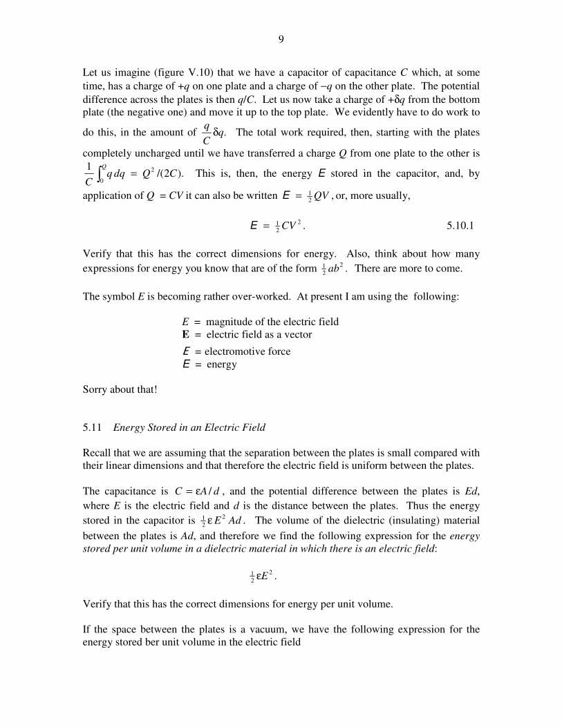
Let us imagine (figure V.10) that we have a capacitor of capacitance C which, at some

time, has a charge of +q on one plate and a charge of −q on the other plate. The potential

difference across the plates is then q/C. Let us now take a charge of +δq from the bottom

plate (the negative one) and move it up to the top plate. We evidently have to do work to

do this, in the amount of .qC

qδ The total work required, then, starting with the plates

completely uncharged until we have transferred a charge Q from one plate to the other is

).2/(1 2

0CQdqq

C

Q

=∫ This is, then, the energy E stored in the capacitor, and, by

application of Q = CV it can also be written ,21 QV=E or, more usually,

.2

21 CV=E 5.10.1

Verify that this has the correct dimensions for energy. Also, think about how many

expressions for energy you know that are of the form .2

21 ab There are more to come.

The symbol E is becoming rather over-worked. At present I am using the following:

E = magnitude of the electric field

E = electric field as a vector

E = electromotive force

E = energy

Sorry about that!

5.11 Energy Stored in an Electric Field

Recall that we are assuming that the separation between the plates is small compared with

their linear dimensions and that therefore the electric field is uniform between the plates.

The capacitance is dAC /ε= , and the potential difference between the plates is Ed,

where E is the electric field and d is the distance between the plates. Thus the energy

stored in the capacitor is .2

21 AdEε The volume of the dielectric (insulating) material

between the plates is Ad, and therefore we find the following expression for the energy

stored per unit volume in a dielectric material in which there is an electric field:

.2

21 Eε

Verify that this has the correct dimensions for energy per unit volume.

If the space between the plates is a vacuum, we have the following expression for the

energy stored ber unit volume in the electric field

10

2

021 Eε

- even though there is absolutely nothing other than energy in the space. Think about

that!

I mentioned in Section 1.7 that in an anisotropic medium D and E are not parallel, the permittivity then

being a tensor quantity. In that case the correct expression for the energy per unit volume in an electric

field is .2

1ED •

5.12 Force Between the Plates of a Plane Parallel Plate Capacitor

We imagine a capacitor with a charge +Q on one plate and −Q on the other, and initially

the plates are almost, but not quite, touching. There is a force F between the plates. Now

we gradually pull the plates apart (but the separation remains small enough that it is still

small compared with the linear dimensions of the plates and we can maintain our

approximation of a uniform field between the plates, and so the force remains F as we

separate them). The work done in separating the plates from near zero to d is Fd, and

this must then equal the energy stored in the capacitor, .21 QV The electric field between

the plates is E = V/d, so we find for the force between the plates

.21 QEF = 5.12.1

We can now do an interesting imaginary experiment, just to see that we understand the

various concepts. Let us imagine that we have a capacitor in which the plates are

horizontal; the lower plate is fixed, while the upper plate is suspended above it from a

spring of force constant k. We connect a battery across the plates, so the plates will

attract each other. The upper plate will move down, but only so far, because the

electrical attraction between the plates is countered by the tension in the spring.

Calculate the equilibrium separation x between the plates as a function of the applied

voltage V. (Horrid word! We don’t say “metreage” for length, “kilogrammage” for mass

or “secondage” for time – so why do we say “voltage” for potential difference and

“acreage” for area? Ugh!) We should be able to use our invention as a voltmeter – it

even has an infinite resistance!

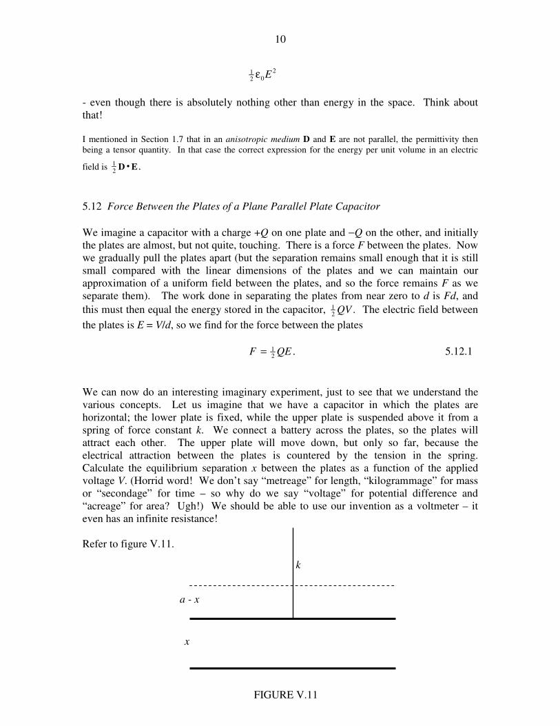
Refer to figure V.11.

k

x

a - x

FIGURE V.11

11

We’ll suppose that the separation when the potential difference is zero is a, and the

separation when the potential difference is V is x, at which time the spring has been

extended by a length a − x.

The electrical force between the plates is QE21 . Now ,and0

x

VE

x

AVCVQ =

ε==

so the force between the plates is .2 2

20

x

AVε Here A is the area of each plate and it is

assumed that the experiment is done in air, whose permittivity is very close to ε0. The

tension in the stretched spring is k(a − x), so equating the two forces gives us

.)(2

0

22

A

xakxV

ε

−= 5.12.2

Calculus shows [do it! – just differentiate x2(1 - x)] that V has a maximum value of

A

kaV

0

3

max27

8

ε= for a separation .

32 ax = If we express the potential difference in units

of maxV and the separation in units of a, equation 5.12.2 becomes

.4

)1(27 22 xx

V−

= 5.12.3

In figure V.12 I have plotted the separation as a function of the potential difference.

12

0 0.2 0.4 0.6 0.8 10

0.1

0.2

0.3

0.4

0.5

0.6

0.7

0.8

0.9

1

V/Vmax

x/a

FIGURE V.10

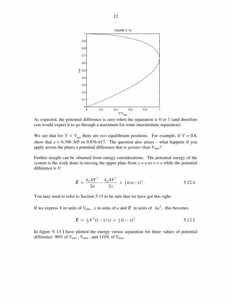
As expected, the potential difference is zero when the separation is 0 or 1 (and therefore

you would expect it to go through a maximum for some intermediate separation).

We see that for maxVV < there are two equilibrium positions. For example, if V = 0.8,

show that x = 0.396 305 or 0.876 617. The question also arises – what happens if you

apply across the plates a potential difference that is greater than Vmax?

Further insight can be obtained from energy considerations. The potential energy of the

system is the work done in moving the upper plate from x = a to x = x while the potential

difference is V:

.)(22

2

21

2

0

2

0 xakx

AV

a

AV−+

ε−

ε=E 5.12.4

You may need to refer to Section 5.15 to be sure that we have got this right.

If we express V in units of Vmax , x in units of a and E in units of ,2ka this becomes

.)1()/11( 2

212

274 xxV −+−=E 5.12.5

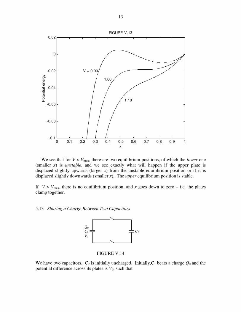
In figure V.13 I have plotted the energy versus separation for three values of potential

difference: 90% of Vmax , Vmax , and 110% of Vmax.

13

0 0.1 0.2 0.3 0.4 0.5 0.6 0.7 0.8 0.9 1-0.1

-0.08

-0.06

-0.04

-0.02

0

0.02

x

Pote

ntial energ

y

FIGURE V.13

V = 0.90

1.00

1.10

We see that for V < Vmax, there are two equilibrium positions, of which the lower one

(smaller x) is unstable, and we see exactly what will happen if the upper plate is

displaced slightly upwards (larger x) from the unstable equilibrium position or if it is

displaced slightly downwards (smaller x). The upper equilibrium position is stable.

If V > Vmax, there is no equilibrium position, and x goes down to zero – i.e. the plates

clamp together.

5.13 Sharing a Charge Between Two Capacitors

We have two capacitors. C2 is initially uncharged. Initially,C1 bears a charge Q0 and the

potential difference across its plates is V0, such that

Q0

C1

V0

FIGURE V.14

C2

14

,010 VCQ = 5.13.1

and the energy of the system is

.2012

10 VC=E 5.13.2

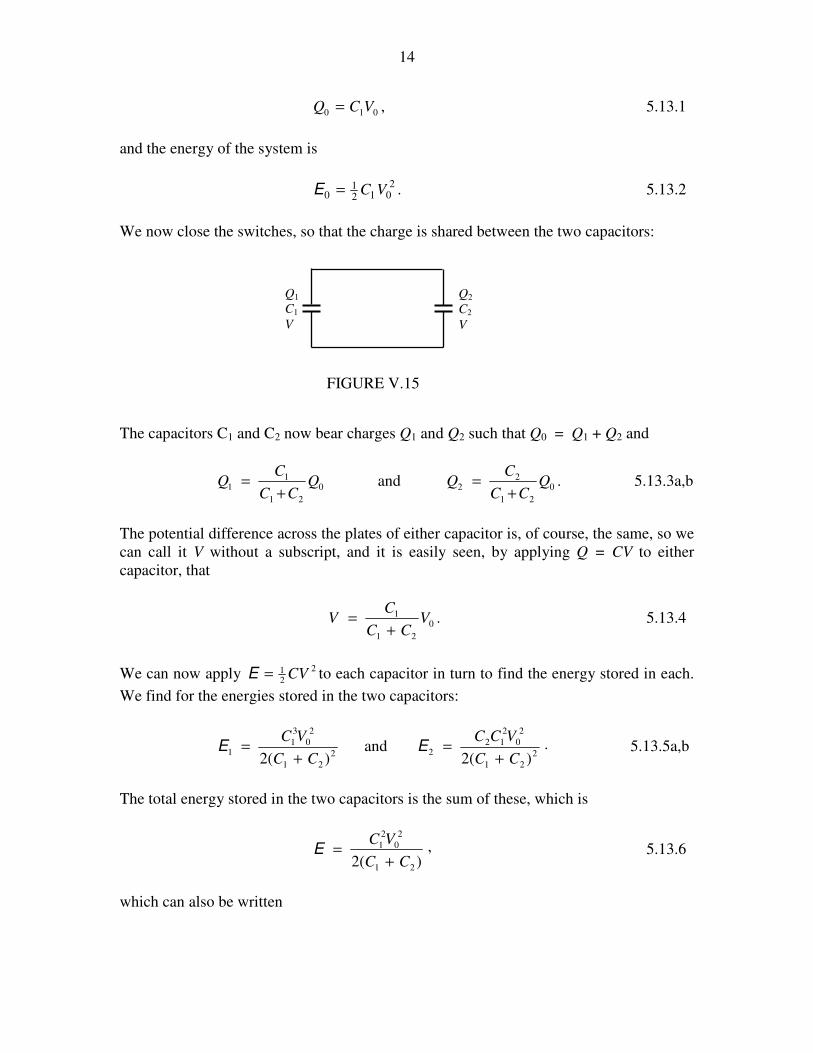
We now close the switches, so that the charge is shared between the two capacitors:

The capacitors C1 and C2 now bear charges Q1 and Q2 such that Q0 = Q1 + Q2 and

0

21

11 Q

CC

CQ

+= and .0

21

22 Q

CC

CQ

+= 5.13.3a,b

The potential difference across the plates of either capacitor is, of course, the same, so we

can call it V without a subscript, and it is easily seen, by applying Q = CV to either

capacitor, that

.0

21

1 VCC

CV

+= 5.13.4

We can now apply 2

21 CV=E to each capacitor in turn to find the energy stored in each.

We find for the energies stored in the two capacitors:

2

21

2

0

3

11

)(2 CC

VC

+=E and .

)(2 2

21

2

0

2

122

CC

VCC

+=E 5.13.5a,b

The total energy stored in the two capacitors is the sum of these, which is

,)(2 21

2

0

2

1

CC

VC

+=E 5.13.6

which can also be written

Q1

C1

V

FIGURE V.15

Q2

C2

V

15

.0

21

1EE

CC

C

+= 5.13.7

Surprise, surprise! The energy stored in the two capacitors is less than the energy that

was originally stored in C1. What has happened to the lost energy?

A perfectly reasonable and not incorrect answer is that it has been dissipated as heat in

the connecting wires as current flowed from one capacitor to the other. However, it has

been found in low temperature physics that if you immerse certain metals in liquid

helium they lose all electrical resistance and they become superconductive. So, let us

connect the capacitors with superconducting wires. Then there is no dissipation of

energy as heat in the wires – so the question remains: where has the missing energy

gone?

Well, perhaps the dielectric medium in the capacitors is heated? Again this seems like a

perfectly reasonable and probably not entirely incorrect answer. However, my capacitors

have a vacuum between the plates, and are connected by superconducting wires, so that

no heat is generated either in the dielectric or in the wires. Where has that energy gone?

This will have to remain a mystery for the time being, and a topic for lunchtime

conversation. In a later chapter I shall suggest another explanation.

5.14 Mixed Dielectrics

This section addresses the question: If there are two or more dielectric media between

the plates of a capacitor, with different permittivities, are the electric fields in the two

media different, or are they the same? The answer depends on

1. Whether by “electric field” you mean E or D;

2. The disposition of the media between the plates – i.e. whether the two

dielectrics are in series or in parallel.

Let us first suppose that two media are in series (figure V.16).

FIGURE V.16

0

V0

V

d1 ε1

D

E1

d2 ε2

E2

Area = A

16

Our capacitor has two dielectrics in series, the first one of thickness d1 and permittivity ε1

and the second one of thickness d2 and permittivity ε2. As always, the thicknesses of the

dielectrics are supposed to be small so that the fields within them are uniform. This is

effectively two capacitors in series, of capacitances ./and/ 2211 dAdA εε The total

capacitance is therefore

.

2112

21

dd

AC

ε+ε

εε= 5.14.1

Let us imagine that the potential difference across the plates is V0. Specifically, we’ll

suppose the potential of the lower plate is zero and the potential of the upper plate is V0.

The charge Q held by the capacitor (positive on one plate, negative on the other) is just

given by Q = CV0, and hence the surface charge density σ is CV0/A. Gauss’s law is that

the total D-flux arising from a charge is equal to the charge, so that in this geometry D =

σ, and this is not altered by the nature of the dielectric materials between the plates.

Thus, in this capacitor, D = CV0/A = Q/A in both media. Thus D is continuous across the

boundary.

Then by application of D = εE to each of the media, we find that the E-fields in the two

media are ,)/(and)/( 2211 AQEAQE ε=ε= the E-field (and hence the potential

gradient) being larger in the medium with the smaller permittivity.

The potential V at the media boundary is given by ./ 22 EdV = Combining this with our

expression for E2, and Q = CV and equation 5.14.1, we find for the boundary potential:

.0

2112

21V

dd

dV

ε+ε

ε= 5.14.2

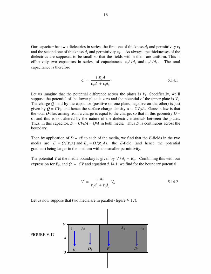
Let us now suppose that two media are in parallel (figure V.17).

0

d

E D1

ε2 ε1

FIGURE V.17

V A1 A2

D2 E

17

This time, we have two dielectrics, each of thickness d, but one has area A1 and

permittivity ε1 while the other has area A2 and permittivity ε2. This is just two capacitors

in parallel, and the total capacitance is

.2211

d

A

d

AC

ε+

ε= 5.14.3

The E-field is just the potential gradient, and this is independent of any medium between

the plates, so that E = V/d. in each of the two dielectrics. After that, we have simply that

.and 2211 EDED ε=ε= The charge density on the plates is given by Gauss’s law as σ

= D, so that, if ε1 < ε2, the charge density on the left hand portion of each plate is less

than on the right hand portion – although the potential is the same throughout each plate.

(The surface of a metal is always an equipotential surface.) The two different charge

densities on each plate is a result of the different polarizations of the two dielectrics –

something that will be more readily understood a little later in this chapter when we deal

with media polarization.

We have established that:

1. The component of D perpendicular to a boundary is continuous;

2. The component of E parallel to a boundary is continuous.

In figure V.18 we are looking at the D-field and at the E-field as it crosses a boundary in

which ε1 < ε2. Note that Dy and Ex are the same on either side of the boundary. This

results in:

.tan

tan

2

1

2

1

ε

ε=

θ

θ 5.14.4

ε1

ε2

ε1Ey/ε2

Dx

Dy

θ1

θ2

Dy

ε2Dx/ε1

Ex

Ey

θ1

θ2

Ex

FIGURE V.18

18

5.15 Changing the Distance Between the Plates of a Capacitor

If you gradually increase the distance between the plates of a capacitor (although always

keeping it sufficiently small so that the field is uniform) does the intensity of the field

change or does it stay the same? If the former, does it increase or decrease?

The answers to these questions depends

1. on whether, by the field, you are referring to the E-field or the D-field;

2. on whether the plates are isolated or if they are connected to the poles of a battery.

We shall start by supposing that the plates are isolated.

In this case the charge on the plates is constant, and so is the charge density. Gauss’s law

requires that D = σ, so that D remains constant. And, since the permittivity hasn’t

changed, E also remains constant.

The potential difference across the plates is Ed, so, as you increase the plate separation,

so the potential difference across the plates in increased. The capacitance decreases

from εA/d1 to εA/d2 and the energy stored in the capacitor increases from

.2

to2

22

21

ε

σ

ε

σ AdAd This energy derives from the work done in separating the plates.

Now let’s suppose that the plates are connected to a battery of EMF V, with air or a

vacuum between the plates. At first, the separation is d1. The magnitudes of E and D are,

respectively, V/d1 and ε0V/d1. When we have increased the separation to d2, the potential

difference across the plates has not changed; it is still the EMF V of the battery. The

electric field, however, is now only E = V/d2 and D = ε0V/d2. But Gauss’s law still

dictates that D = σ, and therefore the charge density, and the total charge on the plates, is

less than it was before. It has gone into the battery. In other words, in doing work by

separating the plates we have recharged the battery. The energy stored in the capacitor

was originally ;2 1

2

0

d

AVε it is now only .

2 2

2

0

d

AVε Thus the energy held in the capacitor has

been reduced by .11

21

2

021

−ε

ddAV

The charge originally held by the capacitor was .1

0

d

AVε After the plate separation has

been increased to d2 the charge held is .2

0

d

AVε The difference,

−ε

21

0

11

ddAV , is the

19

charge that has gone into the battery. The energy, or work, required to force this amount

of charge into the battery against its EMF V is .11

21

2

0

−ε

ddAV Half of this came from

the loss in energy held by the capacitor (see above). The other half presumably came

from the mechanical work you did in separating the plates. Let’s see if we can verify

this.

When the plate separation is x, the force between the plates is ,21 QE which is

.2

or.2

2

00

21

x

AV

x

V

x

AV εε The work required to increase x from d1 to d2 is

,2

2

12

2

0 ∫ε d

d x

dxAV which is indeed .

11

21

2

021

−ε

ddAV Thus this amount of mechanical

work, plus an equal amount of energy from the capacitor, has gone into recharging the

battery. Expressed otherwise, the work done in separating the plates equals the work

required to charge the battery minus the decrease in energy stored by the capacitor.

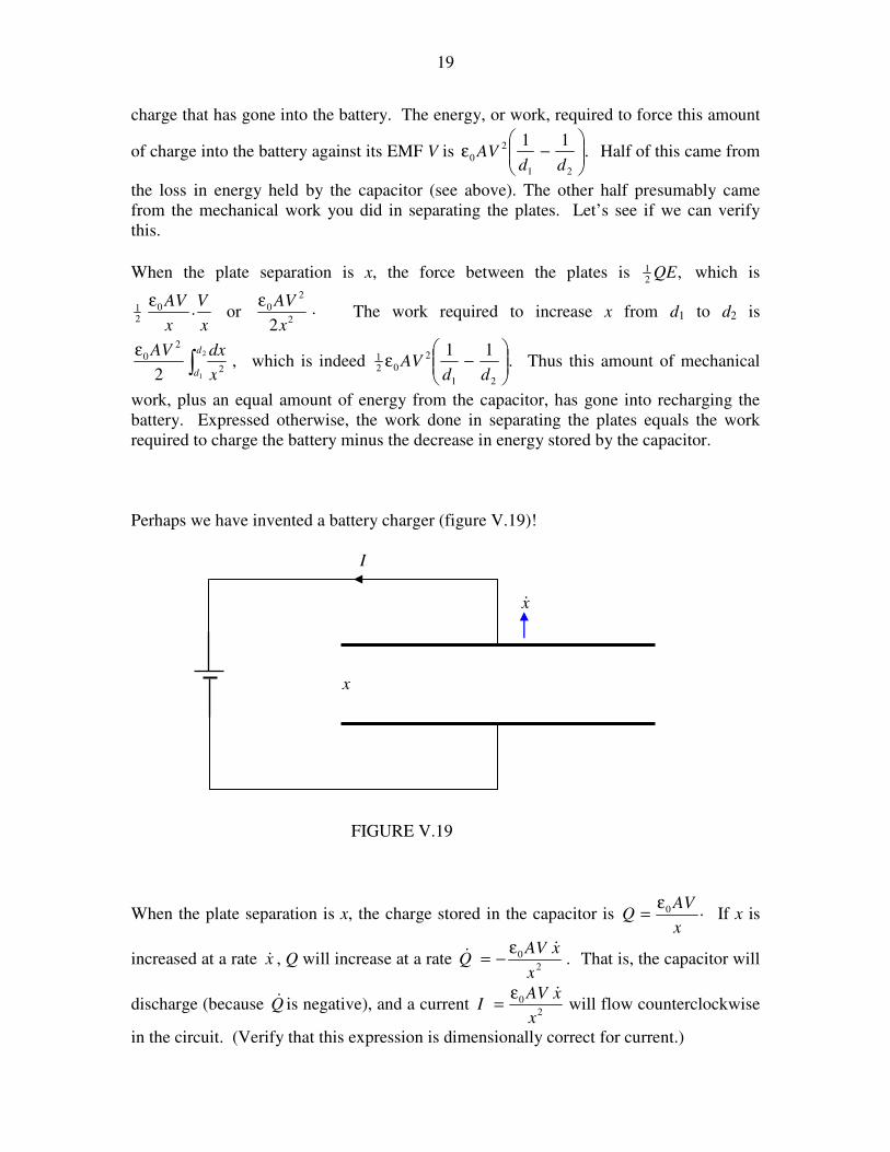
Perhaps we have invented a battery charger (figure V.19)!

When the plate separation is x, the charge stored in the capacitor is .0

x

AVQ

ε= If x is

increased at a rate x& , Q will increase at a rate .2

0

x

xAVQ

&&

ε−= That is, the capacitor will

discharge (because Q& is negative), and a current 2

0

x

xAVI

&ε= will flow counterclockwise

in the circuit. (Verify that this expression is dimensionally correct for current.)

x

I

FIGURE V.19

x&

20

5.16 Inserting a Dielectric into a Capacitor

Suppose you start with two plates separated by a vacuum or by air, with a potential

difference across the plates, and you then insert a dielectric material of permittivity ε0

between the plates. Does the intensity of the field change or does it stay the same? If the

former, does it increase or decrease?

The answer to these questions depends

1. on whether, by the field, you are referring to the E-field or the D-field;

2. on whether the plates are isolated or if they are connected to the poles of a battery.

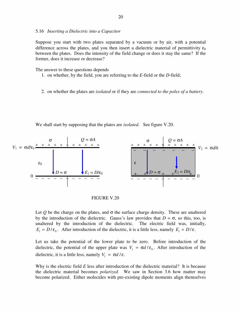
We shall start by supposing that the plates are isolated. See figure V.20.

Let Q be the charge on the plates, and σ the surface charge density. These are unaltered

by the introduction of the dielectric. Gauss’s law provides that D = σ, so this, too, is

unaltered by the introduction of the dielectric. The electric field was, initially,

./ 01 ε= DE After introduction of the dielectric, it is a little less, namely ./1 ε= DE

Let us take the potential of the lower plate to be zero. Before introduction of the

dielectric, the potential of the upper plate was ./ 01 εσ= dV After introduction of the

dielectric, it is a little less, namely ./1 εσ= dV

Why is the electric field E less after introduction of the dielectric material? It is because

the dielectric material becomes polarized. We saw in Section 3.6 how matter may

become polarized. Either molecules with pre-existing dipole moments align themselves

V1 = σd/ε0

FIGURE V.20

− − − − − − − − − − − − − − − − − − − − − −

+ + + + + + + + + + + + + + + + + + + + + +

0

ε ε0

σ Q = σA Q = σA σ

V2 = σd/ε

0

D = σ E2 = D/ε D = σ E1 = D/ε0

− − − − − − −

+ + + + +

21

with the imposed electric field, or, if they have no permanent dipole moment or if they

cannot rotate, a dipole moment can be induced in the individual molecules. In any case,

the effect of the alignment of all these molecular dipoles is that there is a slight surplus of

positive charge on the surface of the dielectric material next to the negative plate, and a

slight surplus of negative charge on the surface of the dielectric material next to the

positive plate. This produces an electric field opposite to the direction of the imposed

field, and thus the total electric field is somewhat reduced.

Before introduction of the dielectric material, the energy stored in the capacitor was

121 QV . After introduction of the material, it is ,22

1 QV which is a little bit less. Thus it

will require work to remove the material from between the plates. The empty capacitor

will tend to suck the material in, just as the charged rod in Chapter 1 attracted an

uncharged pith ball.

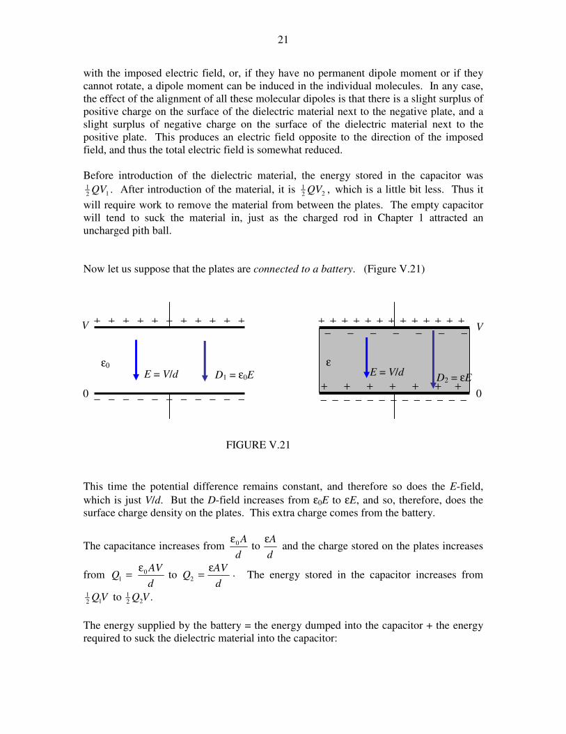
Now let us suppose that the plates are connected to a battery. (Figure V.21)

This time the potential difference remains constant, and therefore so does the E-field,

which is just V/d. But the D-field increases from ε0E to εE, and so, therefore, does the

surface charge density on the plates. This extra charge comes from the battery.

The capacitance increases from d

A

d

A εεto0 and the charge stored on the plates increases

from .to 20

1d

AVQ

d

AVQ

ε=

ε= The energy stored in the capacitor increases from

.to 221

121 VQVQ

The energy supplied by the battery = the energy dumped into the capacitor + the energy

required to suck the dielectric material into the capacitor:

V

FIGURE V.21

− − − − − − − − − − − − − − − − − − − − − − − −

+ + + + + + + + + + + + + + + + + + + + + + + +

0

ε ε0

V

0

D2 = εE E = V/d D1 = ε0E

− − − − − − −

+ + + + + + +

E = V/d

22

.)()()( 1221

1221

12 VQQVQQVQQ −+−=−

You would have to do work to remove the material from the capacitor; half of the work

you do would be the mechanical work performed in pulling the material out; the other

half would be used in charging the battery.

In Section 5.15 I invented one type of battery charger. I am now going to make my

fortune by inventing another type of battery charger.

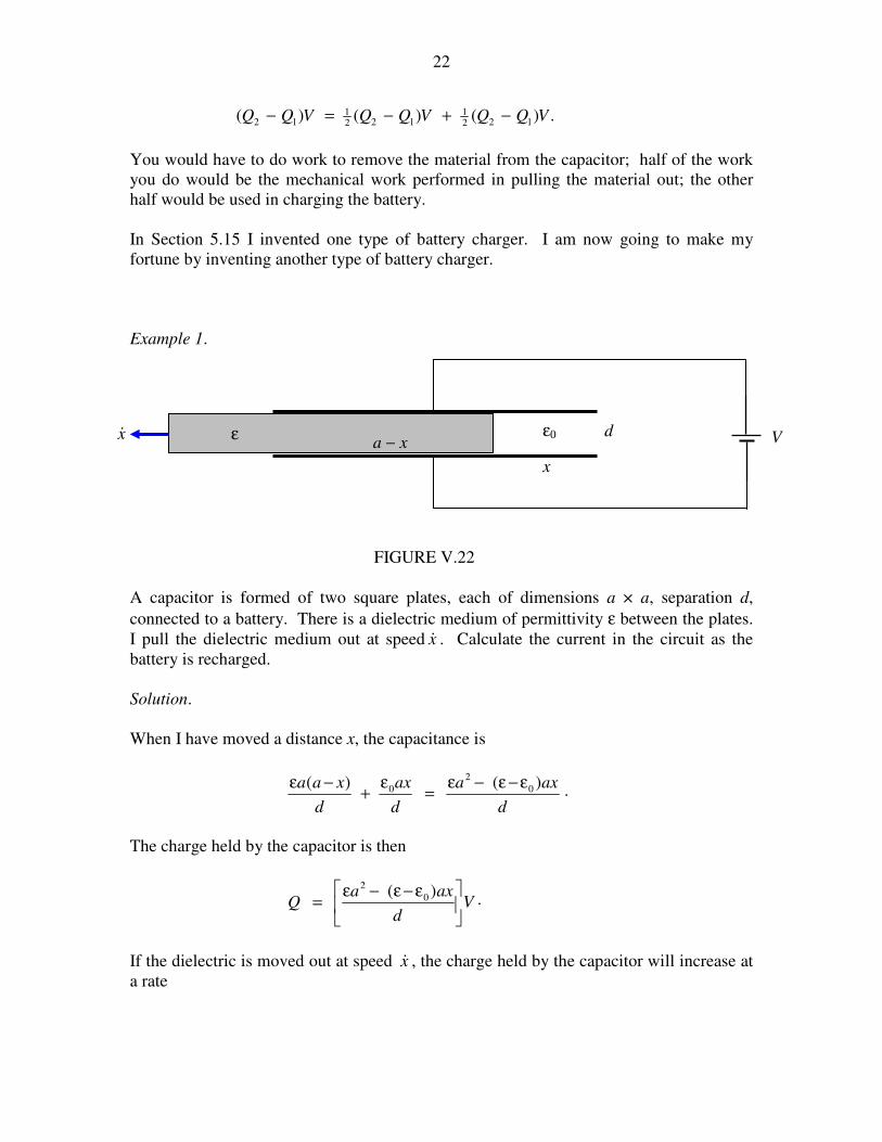
Example 1.

A capacitor is formed of two square plates, each of dimensions a × a, separation d,

connected to a battery. There is a dielectric medium of permittivity ε between the plates.

I pull the dielectric medium out at speed x& . Calculate the current in the circuit as the

battery is recharged.

Solution.

When I have moved a distance x, the capacitance is

.)()( 0

2

0

d

axa

d

ax

d

xaa ε−ε−ε=

ε+

−ε

The charge held by the capacitor is then

.)( 0

2

Vd

axaQ

ε−ε−ε=

If the dielectric is moved out at speed x& , the charge held by the capacitor will increase at

a rate

ε ε0 x&

x

a − x d

FIGURE V.22

V

23

.)( 0

d

VxaQ

&&

ε−ε−=

(That’s negative, so Q decreases.) A current of this magnitude therefore flows clockwise

around the circuit, into the battery. You should verify that the expression has the correct

dimensions for current.

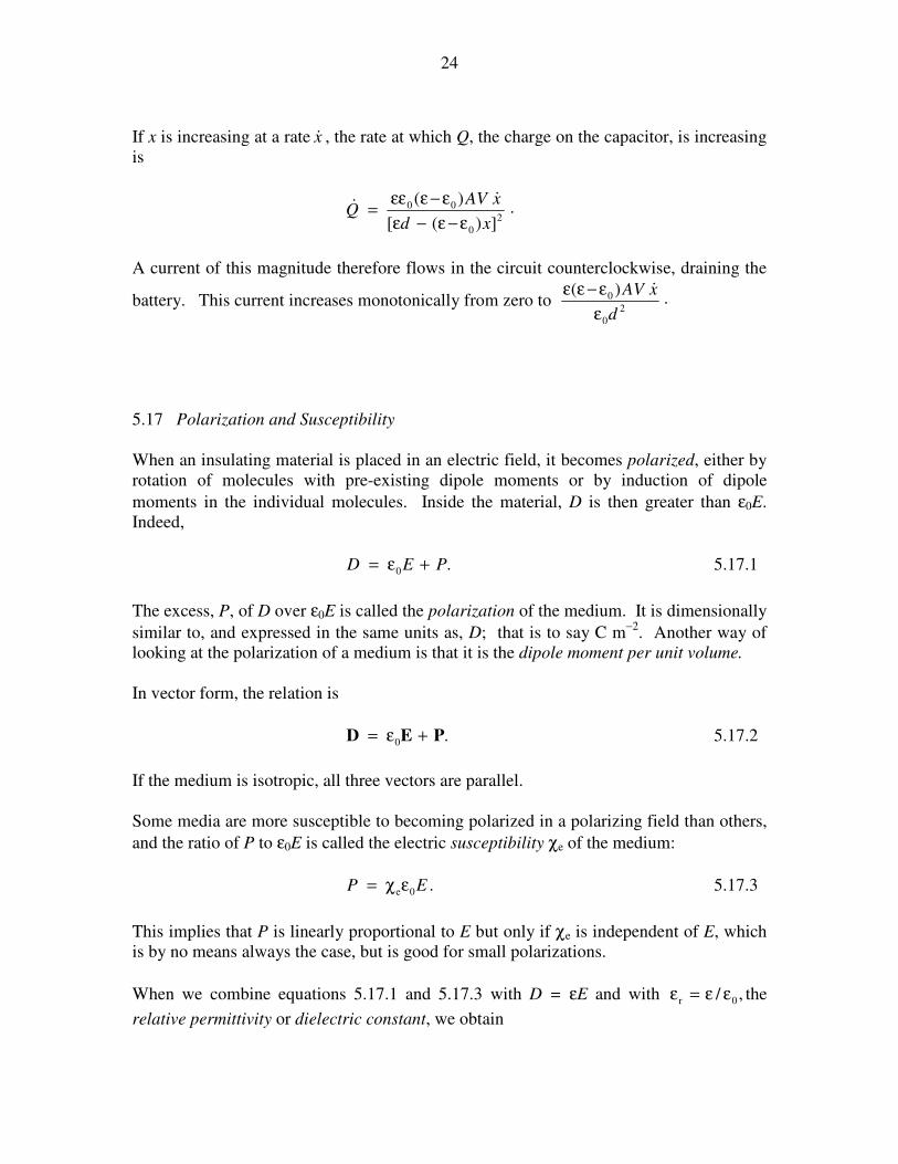
Example 2.

A capacitor consists of two plates, each of area A, separated by a distance x, connected to

a battery of EMF V. A cup rests on the lower plate. The cup is gradually filled with a

nonconducting liquid of permittivity ε, the surface rising at a speed x& . Calculate the

magnitude and direction of the current in the circuit.

It is easy to calculate that, when the liquid has a depth x, the capacitance of the capacitor

is

xd

AC

)( 0

0

ε−ε−ε

εε=

and the charge held by the capacitor is then

.)( 0

0

xd

AVQ

ε−ε−ε

εε=

FIGURE V.23

d − x

x

V

ε0

x&

ε

24

If x is increasing at a rate x& , the rate at which Q, the charge on the capacitor, is increasing

is

.])([

)(2

0

00

xd

xAVQ

ε−ε−ε

ε−εεε=

&&

A current of this magnitude therefore flows in the circuit counterclockwise, draining the

battery. This current increases monotonically from zero to .)(2

0

0

d

xAV

ε

ε−εε &

5.17 Polarization and Susceptibility

When an insulating material is placed in an electric field, it becomes polarized, either by

rotation of molecules with pre-existing dipole moments or by induction of dipole

moments in the individual molecules. Inside the material, D is then greater than ε0E.

Indeed,

.0 PED +ε= 5.17.1

The excess, P, of D over ε0E is called the polarization of the medium. It is dimensionally

similar to, and expressed in the same units as, D; that is to say C m−2

. Another way of

looking at the polarization of a medium is that it is the dipole moment per unit volume.

In vector form, the relation is

.0 PED +ε= 5.17.2

If the medium is isotropic, all three vectors are parallel.

Some media are more susceptible to becoming polarized in a polarizing field than others,

and the ratio of P to ε0E is called the electric susceptibility χe of the medium:

.0e EP εχ= 5.17.3

This implies that P is linearly proportional to E but only if χe is independent of E, which

is by no means always the case, but is good for small polarizations.

When we combine equations 5.17.1 and 5.17.3 with D = εE and with ,/ 0r εε=ε the

relative permittivity or dielectric constant, we obtain

25

.1re −ε=χ 5.17.4

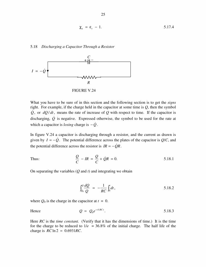
5.18 Discharging a Capacitor Through a Resistor

What you have to be sure of in this section and the following section is to get the signs

right. For example, if the charge held in the capacitor at some time is Q, then the symbol

,/or, dtdQQ& means the rate of increase of Q with respect to time. If the capacitor is

discharging, Q& is negative. Expressed otherwise, the symbol to be used for the rate at

which a capacitor is losing charge is Q&− .

In figure V.24 a capacitor is discharging through a resistor, and the current as drawn is

given by .QI &−= The potential difference across the plates of the capacitor is Q/C, and

the potential difference across the resistor is .RQIR &−=

Thus: .0=+=− RQC

QIR

C

Q& 5.18.1

On separating the variables (Q and t) and integrating we obtain

,1

00∫∫ −=

tQ

Qdt

RCQ

dQ 5.18.2

where Q0 is the charge in the capacitor at t = 0.

Hence .)/(

0

RCteQQ

−= 5.18.3

Here RC is the time constant. (Verify that it has the dimensions of time.) It is the time

for the charge to be reduced to 1/e = 36.8% of the initial charge. The half life of the

charge is .6931.02ln RCRC =

FIGURE V.24

R

+ −

QI &−=

C

26

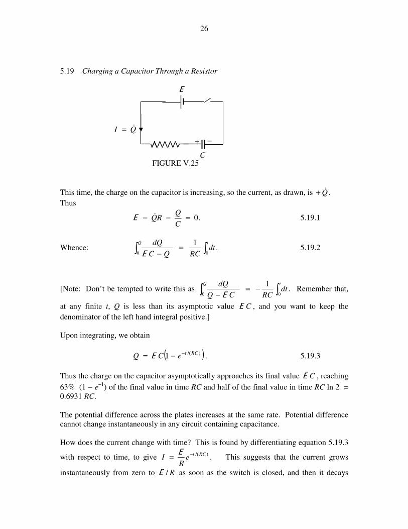
5.19 Charging a Capacitor Through a Resistor

This time, the charge on the capacitor is increasing, so the current, as drawn, is .Q&+

Thus

.0=−−C

QRQ&E 5.19.1

Whence: ∫∫ =−

tQ

dtRCQC

dQ

00.

1

E 5.19.2

[Note: Don’t be tempted to write this as ∫∫ −=−

tQ

dtRCCQ

dQ

00.

1

E Remember that,

at any finite t, Q is less than its asymptotic value CE , and you want to keep the

denominator of the left hand integral positive.]

Upon integrating, we obtain

( ) .1 )/(RCteCQ −−= E 5.19.3

Thus the charge on the capacitor asymptotically approaches its final value CE , reaching

63% (1 − e−1

) of the final value in time RC and half of the final value in time RC ln 2 =

0.6931 RC.

The potential difference across the plates increases at the same rate. Potential difference

cannot change instantaneously in any circuit containing capacitance.

How does the current change with time? This is found by differentiating equation 5.19.3

with respect to time, to give )/(RCte

RI

−=E

. This suggests that the current grows

instantaneously from zero to R/E as soon as the switch is closed, and then it decays

QI &=

FIGURE V.25 C

E

+ −

27

exponentially, with time constant RC, to zero. Is this really possible? It is possible in

principle if the inductance (see Chapter 12) of the circuit is zero. But the inductance of

any closed circuit cannot be exactly zero, and the circuit, as drawn without any

inductance whatever, is not achievable in any real circuit, and so, in a real circuit, there

will not be an instantaneous change of current. Chapter 10 Section 10.15 will deal with

the growth of current in a circuit that contains both capacitance and inductance as well as

resistance.

Energy considerations

When the capacitor is fully charged, the current has dropped to zero, the potential

difference across its plates is E (the EMF of the battery), and the energy stored in the

capacitor (see Section 5.10) is EE QC212

21 = . But the energy lost by the battery is EQ .

Let us hope that the remaining EQ21 is heat generated in and dissipated by the resistor.

The rate at which heat is generated by current in a resistor (see Chapter 4 Section 4.6) is

RI 2 . In this case, according to the previous paragraph, the current at time t is

)/(RCte

RI

−=E

, so the total heat generated in the resistor is 221

0

)/(22

EE

CeR

RCt =∫∞

− ,

so all is well. The energy lost by the battery is shared equally between R and C.

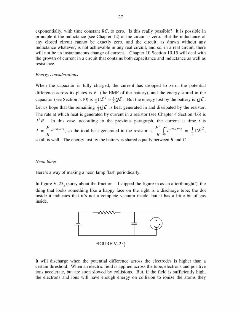
Neon lamp

Here’s a way of making a neon lamp flash periodically.

In figure V.2125 (sorry about the fraction – I slipped the figure in as an afterthought!), the

thing that looks something like a happy face on the right is a discharge tube; the dot

inside it indicates that it’s not a complete vacuum inside, but it has a little bit of gas

inside.

It will discharge when the potential difference across the electrodes is higher than a

certain threshold. When an electric field is applied across the tube, electrons and positive

ions accelerate, but are soon slowed by collisions. But, if the field is sufficiently high,

the electrons and ions will have enough energy on collision to ionize the atoms they

FIGURE V.2125

28

collide with, so a cascading discharge will occur. The potential difference rises

exponentially on an RC time-scale until it reaches the threshold value, and the neon tube

suddenly discharges. Then it starts all over again.

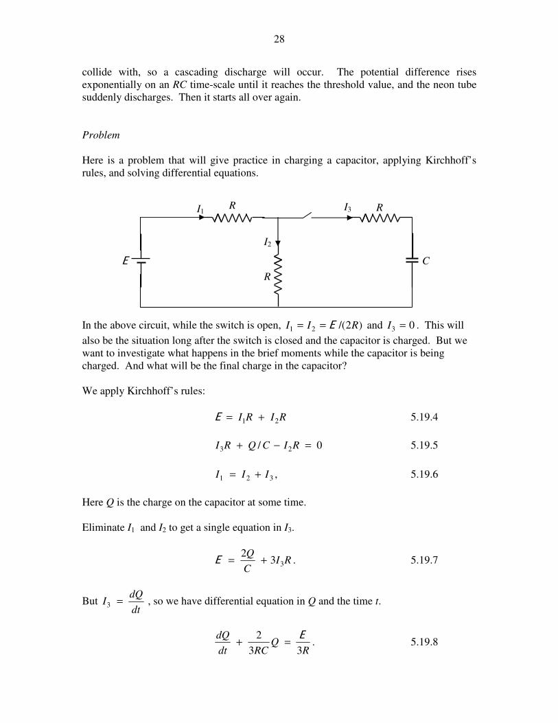
Problem

Here is a problem that will give practice in charging a capacitor, applying Kirchhoff’s

rules, and solving differential equations.

In the above circuit, while the switch is open, )2/(21 RII E== and 03 =I . This will

also be the situation long after the switch is closed and the capacitor is charged. But we

want to investigate what happens in the brief moments while the capacitor is being

charged. And what will be the final charge in the capacitor?

We apply Kirchhoff’s rules:

RIRI 21 +=E 5.19.4

0/ 23 =−+ RICQRI 5.19.5

321 III += , 5.19.6

Here Q is the charge on the capacitor at some time.

Eliminate I1 and I2 to get a single equation in I3.

RIC

Q33

2+=E . 5.19.7

But dt

dQI =3 , so we have differential equation in Q and the time t.

R

QRCdt

dQ

33

2 E=+ . 5.19.8

C E

R R

R

I1 I3

I2

29

This is of the form baydx

dy=+ , and those experienced with differential equations will

have no difficulty in arriving at the solution

RC

t

AeCQ 3

2

21

−

+= E 5.19.9

With the initial condition that Q = 0 when t = 0, this becomes

−=

−RC

t

eCQ 3

2

21 1E . 5.19.10

Thus the final charge in the capacitor is CE21 .

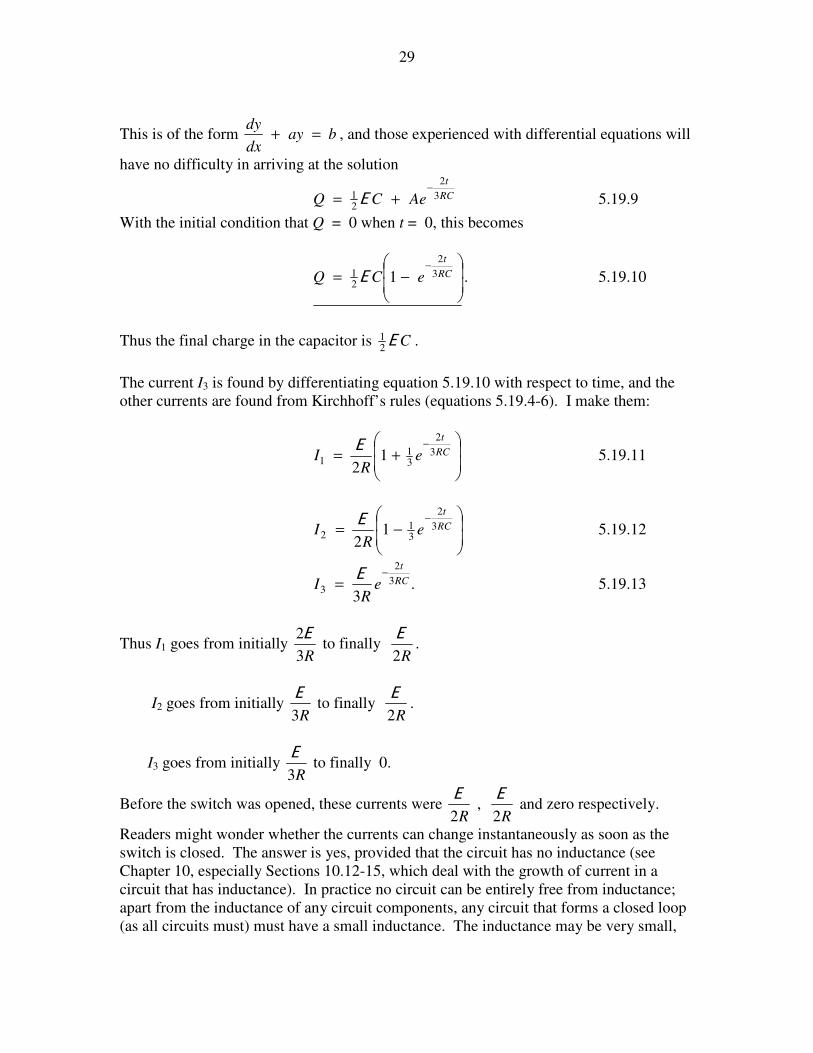
The current I3 is found by differentiating equation 5.19.10 with respect to time, and the

other currents are found from Kirchhoff’s rules (equations 5.19.4-6). I make them:

+=

−RC

t

eR

I 3

2

31

1 12

E 5.19.11

−=

−RC

t

eR

I 3

2

31

2 12

E 5.19.12

.3

3

2

3RC

t

eR

I−

=E

5.19.13

Thus I1 goes from initially R3

2E to finally

R2

E.

I2 goes from initially R3

E to finally

R2

E.

I3 goes from initially R3

E to finally 0.

Before the switch was opened, these currents were R2

E ,

R2

E and zero respectively.

Readers might wonder whether the currents can change instantaneously as soon as the

switch is closed. The answer is yes, provided that the circuit has no inductance (see

Chapter 10, especially Sections 10.12-15, which deal with the growth of current in a

circuit that has inductance). In practice no circuit can be entirely free from inductance;

apart from the inductance of any circuit components, any circuit that forms a closed loop

(as all circuits must) must have a small inductance. The inductance may be very small,

30

which means that the change of current at the instant when the switch is closed is very

rapid. It is not, however, instantaneous.

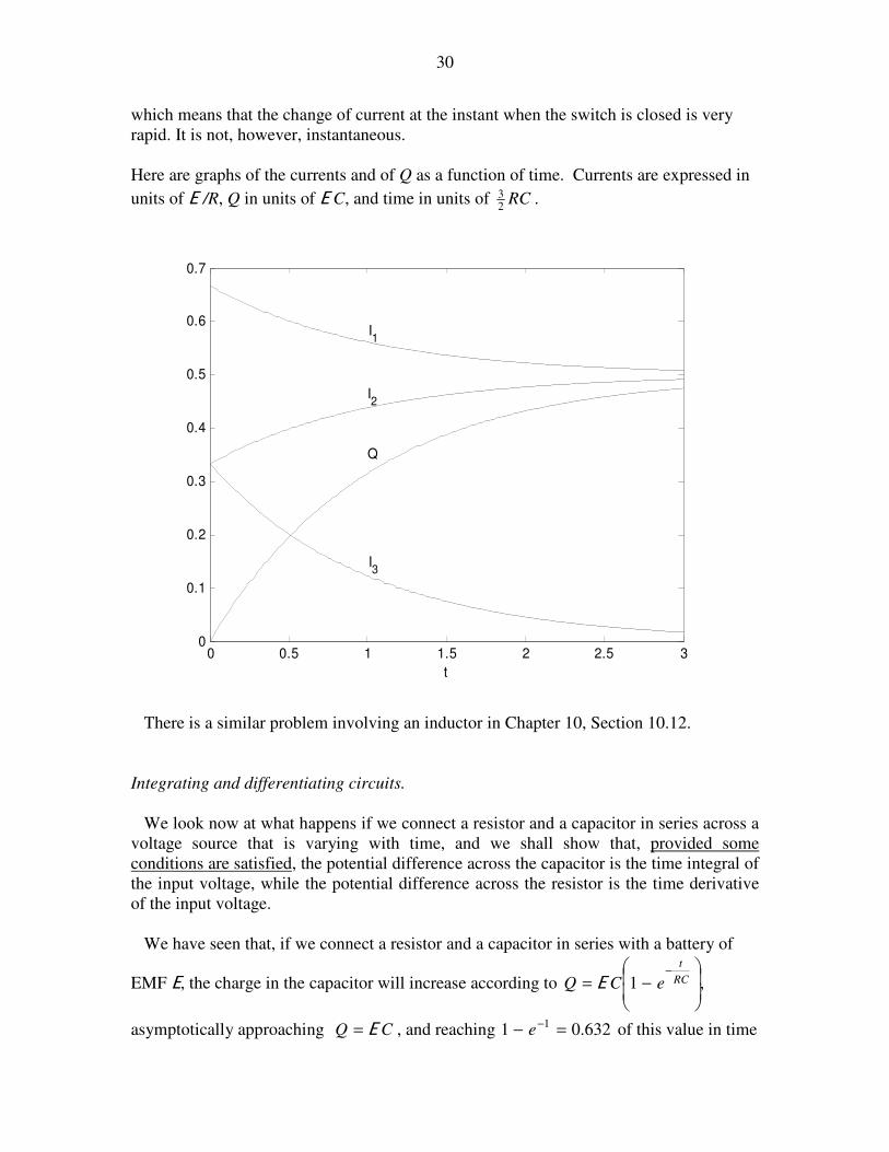
Here are graphs of the currents and of Q as a function of time. Currents are expressed in

units of E /R, Q in units of E C, and time in units of RC23 .

0 0.5 1 1.5 2 2.5 30

0.1

0.2

0.3

0.4

0.5

0.6

0.7

t

I1

I2

I3

Q

There is a similar problem involving an inductor in Chapter 10, Section 10.12.

Integrating and differentiating circuits.

We look now at what happens if we connect a resistor and a capacitor in series across a

voltage source that is varying with time, and we shall show that, provided some

conditions are satisfied, the potential difference across the capacitor is the time integral of

the input voltage, while the potential difference across the resistor is the time derivative

of the input voltage.

We have seen that, if we connect a resistor and a capacitor in series with a battery of

EMF E, the charge in the capacitor will increase according to ,1

−=

−RC

t

eCQ E

asymptotically approaching CQ E= , and reaching 632.01 1 =− −e of this value in time

31

RC. Note that, when RCt << , the current will be large, and the charge in the capacitor

will be small. Most of the potential drop in the circuit will be across the resistor, and

relatively little across the capacitor. After a long time, however, the current will be low,

and the charge will be high, so that most of the potential drop will be across the capacitor,

and relatively little across the resistor. The potential drops across R and C will be equal

at a time .693.02ln RCRCt ==

Suppose that, instead of connecting R and C to a battery of constant EMF, we connect it

to a source whose voltage varies with time, )(tV . How will the charge in C vary with

time?

The relevant equation is CQIRV /+= , in which I, Q and V are all functions of time.

Since QI &= , the differential equation showing how Q varies with time is

R

VQ

RCdt

dQ=+

1 5.19.14

The integration of this equation is made easy if we multiply both sides by RC

t

e . (Those

who are experienced in solving differential equations will readily think of this step.

Those who are less experienced might not immediately think of it, but will soon see that

it is a useful step.) We then obtain

RC

t

RC

t

RC

t

RC

t

eR

VQe

dt

dQe

RCdt

dQe =

=+

1 5.19.15

Thus the answer to our question is

.dtVeR

eQ RC

tRC

t

∫−

= 5.19.16

If V = E and is independent of time, this reduces to the familiar .1

−=

−RC

t

eCQ E

The potential difference across C increases, of course, as

.dtVeRC

eV RC

tRC

t

C ∫−

= 5.19.17

)(tVV = CV

R

C

32

While t is very much shorter than the time constant RC, by which I mean short enough

that RC

t

e is very close to 1, this becomes

.1

VdtRC

VC ∫= 5.19.18

That is why this circuit is called an integrating circuit. The output voltage across C is

)/(1 RC times the time integral of the input voltage V. This is also true if the input

voltage is a periodic function of time with a period that is very much shorter than the time

constant.

By way of example, suppose that 2atV = . If we put this in the right hand side of

equation 5.19.17 and integrate, with initial condition VC = 0 when t = 0, (do it!), we

obtain

.222

22

222

−+−=

−RC

t

C eRC

t

CR

tCaRV 5.19.19

For example, suppose the input voltage varies as 25tV = volts, where t is in seconds. If

R = 500 Ω and C = 400 µF, what will be the potential differnece across the capacitor

after 0.3 s? We immediately see that RC = 0.2 s and )/(RCt = 1.5. Substitute SI

numbers in equation 5.19.19 to obtain VC = 0.161 V.

If I write 22

CaR

Vy C= and

RC

tx = equation 5.19.19 in dimensionless form

becomes

.2222 xexxy −−+−= 5.19.20

If you Taylor expand this as far as x3 (do it!), you get 3

31 xy = , which is just what you

would get by using equation 5.19.18, the equation which is an approximation for a time

that is short compared with RC. The approximation is good as long as

4

RC

tis

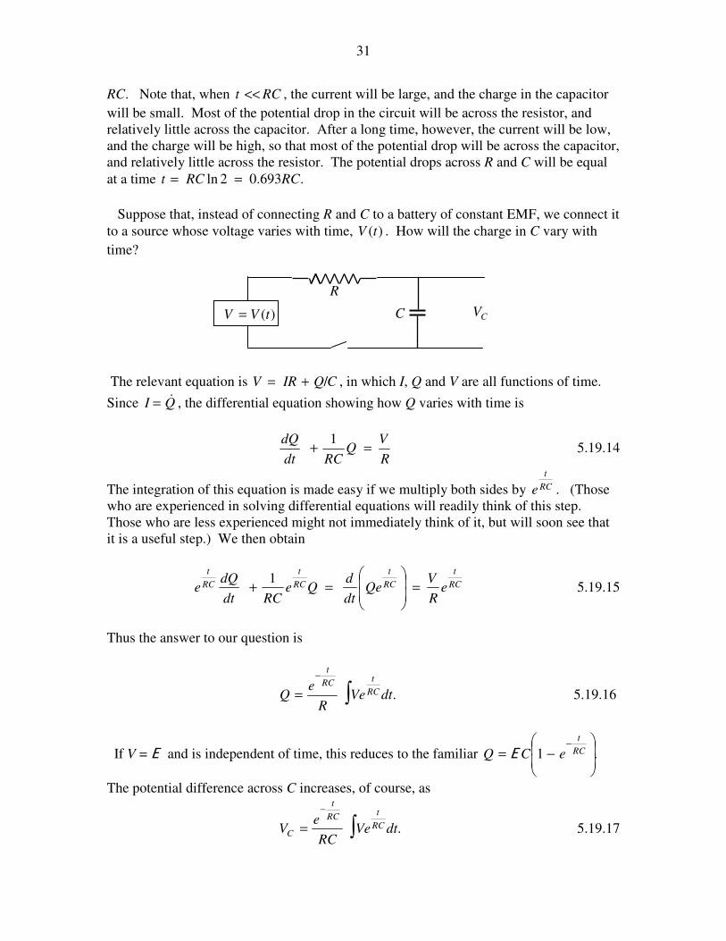
negligible. I show equation 5.19.20 and 3

31 xy = in the graph below, in which VC is in

units of 22CaR and T is in units of RC.

33

0 0.05 0.1 0.15 0.2 0.25 0.3 0.35 0.4 0.45 0.50

0.005

0.01

0.015

0.02

0.025

0.03

0.035

0.04

0.045

time

VC

exact

approximate

Equation 5.19.17 (or, for short time intervals, equation 5.19.18) gives us the voltage

across C as a function of time. What about the voltage across R? That is evidently

.dtVeRC

eVV RC

tRC

t

R ∫−

−= 5.19.21

Differentiate with respect to time:

RC

V

dt

dVVV

RCdt

dV

dtVeRC

eVee

RCdt

dV

dt

dV

RC

RC

tRC

t

RC

t

RC

t

R

−=−−=

−−= ∫−

−

)(1

1

5.19.22

If the time constant is small so that RC

V

dt

dV RR << , this becomes

dR

dVRCVR = , 5.20.23

34

so that the voltage across R is RC times the time derivative of the input voltage V. Thus

we have a differentiating circuit.

Note that, in the integrating circuit, the circuit must have a large time constant (large R

and C) and time variations in V are rapid compared with RC. The output voltage across

C is then .1

VdtRC

∫ In the differentiating circuit, the circuit must have a small time

constant, and time variations in V are slow compared with RC. The output voltage across

R is then dR

dV.

5.20 Real Capacitors

Real capacitors can vary from huge metal plates suspended in oil to the tiny cylindrical

components seen inside a radio. A great deal of information about them is available on

the Web and from manufacturers’ catalogues, and I only make the briefest remarks here.

A typical inexpensive capacitor seen inside a radio is nothing much more than two strips

of metal foil separated by a strip of plastic or even paper, rolled up into a cylinder much

like a Swiss roll. Thus the separation of the “plates” is small, and the area of the plates is

as much as can be conveniently rolled into a tiny radio component.

In most applications it doesn’t matter which way round the capacitor is connected.

However, with some capacitors it is intended that the outermost of the two metal strips be

grounded (“earthed” in UK terminology), and the inner one is shielded by the outer one

from stray electric fields. In that case the symbol used to represent the capacitor is

The curved line is the outer strip, and is the one that is intended to be grounded. It should

be noted, however, that not everyone appears to be aware of this convention or adheres to

it, and some people will use this symbol to denote any capacitor. Therefore care must be

taken in reading the literature to be sure that you know what the writer intended, and, if

you are describing a circuit yourself, you must make very clear the intended meaning of

your symbols.

There is a type of capacitor known as an electrolytic capacitor. The two “plates” are

strips of aluminium foil separated by a conducting paste, or electrolyte. One of the foils

is covered by an extremely thin layer of aluminium oxide, which has been electrolytically

deposited, and it is this layer than forms the dielectric medium, not the paste that

separates the two foils. Because of the extreme thinness of the oxide layer, the

capacitance is relatively high, although it may not be possible to control the actual

thickness with great precision and consequently the actual value of the capacitance may

not be known with great precision. It is very important that an electrolytic capacitor be

corrected the right way round in a circuit, otherwise electrolysis will start to remove the

35

oxide layer from one foil and deposit it on the other, thus greatly changing the

capacitance. Also, when this happens, a current may pass through the electrolyte and

heat it up so much that the capacitor may burst open with consequent danger to the eyes.

The symbol used to indicate an electrolytic capacitor is:

The side indicated with the plus sign (which is often omitted from the symbol) is to be

connected to the positive side of the circuit.

When you tune your radio, you will usually find that, as you turn the knob that changes

the wavelength that you want to receive, you are changing the capacitance of a variable

air-spaced capacitor just behind the knob. A variable capacitor can be represented by the

symbol

Such a capacitor often consists of two sets of interleaved partiallyoverlapping plates, one

set of which can be rotated with respect to the other, thus changing the overlap area and

hence the capacitance.

Thinking about this suggests to me a couple of small problems for you to amuse yourself

with.

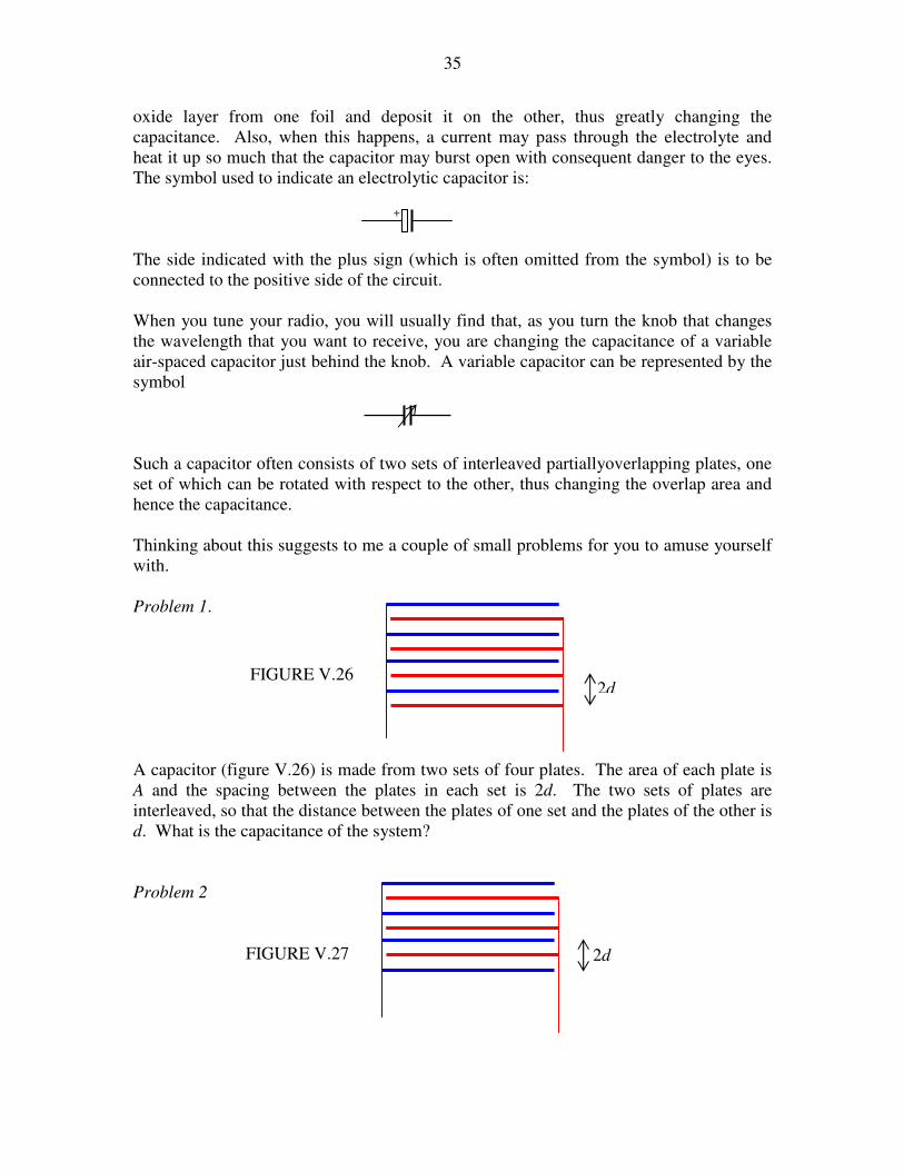
Problem 1.

A capacitor (figure V.26) is made from two sets of four plates. The area of each plate is

A and the spacing between the plates in each set is 2d. The two sets of plates are

interleaved, so that the distance between the plates of one set and the plates of the other is

d. What is the capacitance of the system?

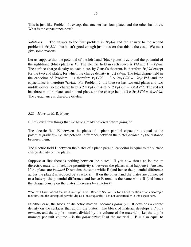
Problem 2

+

FIGURE V.26 2d

FIGURE V.27 2d

36

This is just like Problem 1, except that one set has four plates and the other has three.

What is the capacitance now?

Solutions. The answer to the first problem is 7ε0A/d and the answer to the second

problem is 6ε0A/d – but it isn’t good enough just to assert that this is the case. We must

give some reasons.

Let us suppose that the potential of the left-hand (blue) plates is zero and the potential of

the right-hand (blue) plates is V. The electric field in each space is V/d and D = ε0V/d.

The surface charge density on each plate, by Gauss’s theorem, is therefore 2ε0V/d except

for the two end plates, for which the charge density is just ε0V/d. The total charge held in

the capacitor of Problem 1 is therefore ε0AV/d + 3 × 2ε0AV/d = 7ε0AV/d, and the

capacitance is therefore 7ε0A/d. For Problem 2, the blue set has two end-plates and two

middle-plates, so the charge held is 2 × ε0AV/d + 2 × 2 ε0AV/d = 6ε0AV/d. The red set

has three middle- plates and no end-plates, so the charge held is 3 × 2ε0AV/d = 6ε0AV/d.

The capacitance is therefore 6ε0A/d.

5.21 More on E, D, P, etc.

I’ll review a few things that we have already covered before going on.

The electric field E between the plates of a plane parallel capacitor is equal to the

potential gradient – i.e. the potential difference between the plates divided by the distance

between them.

The electric field D between the plates of a plane parallel capacitor is equal to the surface

charge density on the plates.

Suppose at first there is nothing between the plates. If you now thrust an isotropic*

dielectric material of relative permittivity εr between the plates, what happens? Answer:

If the plates are isolated D remains the same while E (and hence the potential difference

across the plates) is reduced by a factor εr. If on the other hand the plates are connected

to a battery, the potential difference and hence E remains the same while D (and hence

the charge density on the plates) increases by a factor εr.

*You will have noticed the word isotropic here. Refer to Section 1.7 for a brief mention of an anisotropic

medium, and the concept of permittivity as a tensor quantity. I’m not concerned with this aspect here.

In either case, the block of dielectric material becomes polarized. It develops a charge

density on the surfaces that adjoin the plates. The block of material develops a dipole

moment, and the dipole moment divided by the volume of the material – i.e. the dipole

moment per unit volume – is the polarization P of the material. P is also equal to

37

ED 0ε− and, of course, to EE 0ε−ε . The ratio of the resulting polarization P to the

polarizing field ε0E is called the electric susceptibility χ of the medium. It will be worth

spending a few moments convincing yourself from these definitions and concepts that

)1(0 χ+ε=ε and 1r −ε=χ , where rε is the dimensionless relative permittivity (or

dielectric constant) 0/ εε .

What is happening physically inside the medium when it becomes polarized? One

possibility is that the individual molecules, if they are asymmetric molecules, may

already possess a permanent dipole moment. The molecule carbon dioxide, which, in its

ground state, is linear and symmetric, O=C=O, does not have a permanent dipole

moment. Symmetric molecules such as CH4, and single atoms such as He, do not have a

permanent dipole moment. The water molecule has some elements of symmetry, but it

is not linear, and it does have a permanent dipole moment, of about 6 %10−30

C m,

directed along the bisector of the HOH angle and away from the O atom. If the

molecules have a permanent dipole moment and are free to rotate (as, for example, in a

gas) they will tend to rotate in the direction of the applied field. (I’ll discuss that phrase

“tend to” in a moment.) Thus the material becomes polarized.

A molecule such as CH4 is symmetric and has no permanent dipole moment, but, if it is

placed in an external electric field, the molecule may become distorted from its perfect

tetrahedral shape with neat 109º angles, because each pair of CH atoms has a dipole

moment. Thus the molecule acquires an induced dipole moment, and the material as a

whole becomes polarized. The ratio of the induced dipole moment p to the polarizing

field E polarizability α of the molecule. Review Section 3.6 for more on this.

How about a single atom, such as Kr? Even that can acquire a dipole moment. Although

there are no bonds to bend, under the influence of an electric field a preponderance of

electrons will migrate to one side of the atom, and so the atom acquires a dipole moment.

The same phenomenon applies, of course, to a molecule such as CH4 in addition to the

bond bending already mentioned.

Let us consider the situation of a dielectric material in which the molecules have a

permanent dipole moment and are free (as in a gas, for example) to rotate. We’ll suppose

that, at least in a weak polarizing field, the permanent dipole moment is significantly

larger than any induced dipole moment, so we’ll neglect the latter. We have said that,

under the influence of a polarizing field, the permanent dipole will tend to align

themselves with the field. But they also have to contend with the constant jostling and

collisions between molecules, which knock their dipole moments haywire, so they can’t

immediately all align exactly with the field. We might imagine that the material may

become fairly strongly polarized if the temperature is fairly low, but only relatively

weakly polarized at higher temperatures. Dare we even hope that we might be able to

predict the variation of polarization P with temperature T? Let’s have a go!

We recall (Section 3.4) that the potential energy U of a dipole, when it makes an angle θ

with the electric field, is .cos Ep •−=θ−= pEU The energy of a dipole whose

38

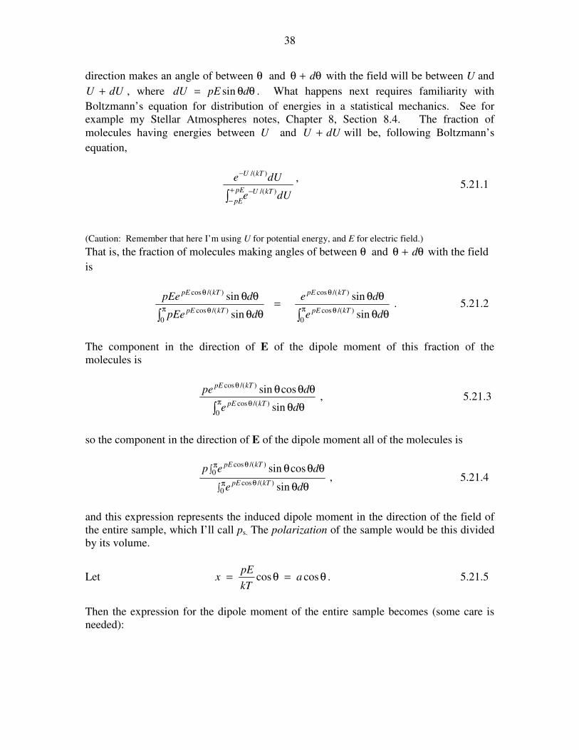
direction makes an angle of between θ and θ+θ d with the field will be between U and

dUU + , where θθ= dpEdU sin . What happens next requires familiarity with

Boltzmann’s equation for distribution of energies in a statistical mechanics. See for

example my Stellar Atmospheres notes, Chapter 8, Section 8.4. The fraction of

molecules having energies between U and dUU + will be, following Boltzmann’s

equation,

∫+

−

−

−

pE

pE

kTU

kTU

dUe

dUe

)/(

)/(

’ 5.21.1

(Caution: Remember that here I’m using U for potential energy, and E for electric field.)

That is, the fraction of molecules making angles of between θ and θ+θ d with the field

is

∫∫π θ

θ

π θ

θ

θθ

θθ=

θθ

θθ

0

)/(cos

)/(cos

0

)/(cos

)/(cos

sin

sin

sin

sin

de

de

dpEe

dpEe

kTpE

kTpE

kTpE

kTpE

. 5.21.2

The component in the direction of E of the dipole moment of this fraction of the

molecules is

∫π θ

θ

θθ

θθθ

0

)/(cos

)/(cos

sin

cossin

de

dpe

kTpE

kTpE

, 5.21.3

so the component in the direction of E of the dipole moment all of the molecules is

∫

∫

π θ

π θ

θθ

θθθ

0)/(cos

0)/(cos

sin

cossin

de

dep

kTpE

kTpE

, 5.21.4

and this expression represents the induced dipole moment in the direction of the field of

the entire sample, which I’ll call ps. The polarization of the sample would be this divided

by its volume.

Let θ=θ= coscos akT

pEx . 5.21.5

Then the expression for the dipole moment of the entire sample becomes (some care is

needed):

39

.1

−

−

+×=×=

−

−

−

+

−

∫

∫aee

eep

dxea

dxxepp

aa

aa

a

a

x

a

a

x

s 5.22.6

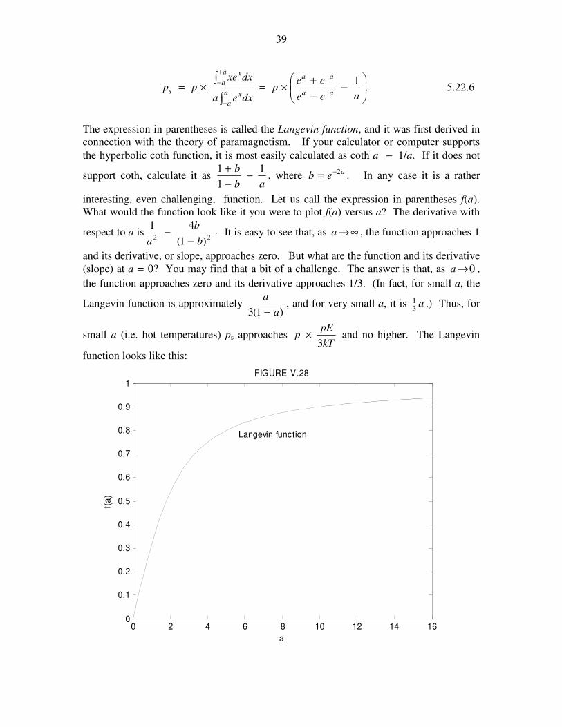
The expression in parentheses is called the Langevin function, and it was first derived in

connection with the theory of paramagnetism. If your calculator or computer supports

the hyperbolic coth function, it is most easily calculated as coth a − 1/a. If it does not

support coth, calculate it as ab

b 1

1

1−

−

+, where aeb 2−= . In any case it is a rather

interesting, even challenging, function. Let us call the expression in parentheses f(a).

What would the function look like it you were to plot f(a) versus a? The derivative with

respect to a is .)1(

4122 b

b

a −− It is easy to see that, as ∞→a , the function approaches 1

and its derivative, or slope, approaches zero. But what are the function and its derivative

(slope) at a = 0? You may find that a bit of a challenge. The answer is that, as 0→a ,

the function approaches zero and its derivative approaches 1/3. (In fact, for small a, the

Langevin function is approximately )1(3 a

a

−, and for very small a, it is a

31 .) Thus, for

small a (i.e. hot temperatures) ps approaches kT

pEp

3× and no higher. The Langevin

function looks like this:

0 2 4 6 8 10 12 14 160

0.1

0.2

0.3

0.4

0.5

0.6

0.7

0.8

0.9

1

a

f(a

)

Langevin function

FIGURE V.28

40

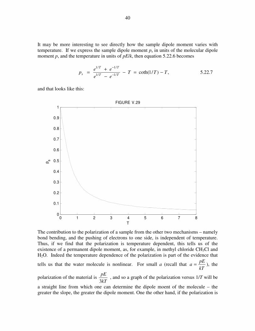
It may be more interesting to see directly how the sample dipole moment varies with

temperature. If we express the sample dipole moment ps in units of the molecular dipole

moment p, and the temperature in units of pE/k, then equation 5.22.6 becomes

,)/1coth(/1/1

/1/1

TTTee

eep

TT

TT

s −=−−

+=

−

−

5.22.7

and that looks like this:

0 1 2 3 4 5 6 7 80

0.1

0.2

0.3

0.4

0.5

0.6

0.7

0.8

0.9

1

T

ps

FIGURE V.29

The contribution to the polarization of a sample from the other two mechanisms – namely

bond bending, and the pushing of electrons to one side, is independent of temperature.

Thus, if we find that the polarization is temperature dependent, this tells us of the

existence of a permanent dipole moment, as, for example, in methyl chloride CH3Cl and

H2O. Indeed the temperature dependence of the polarization is part of the evidence that

tells us that the water molecule is nonlinear. For small a (recall that kT

pEa = ), the

polarization of the material is kT

pE

3 , and so a graph of the polarization versus 1/T will be

a straight line from which one can determine the dipole moent of the molecule – the

greater the slope, the greater the dipole moment. One the other hand, if the polarization is

41

temperature-independent, then the molecule is symmetric, such as methane CH4 and

OCO. Indeed the independence of the polarization on temperature is part of the evidence

that tells us that CO2 is a linear molecule.

5.22 Dielectric material in a alternating electric field.

We have seen that, when we put a dielectric material in an electric field, it becomes

polarized, and the D field is now εE instead of merely ε0E. But how long does it take to

become polarized? Does it happen instantaneously? In practice there is an enormous

range in relaxation times. (We may define a relaxation time as the time taken for the

material to reach a certain fraction – such as, perhaps 631 1 =− −e percent, or whatever

fraction may be convenient in a particular context – of its final polarization.) The

relaxation time may be practically instantaneous, or it may be many hours.

As a consequence of the finite relaxation time, if we put a dielectric material in

oscillating electric field tEE ω= cosˆ (e.g. if light passes through a piece of glass), there

will be a phase lag of D behind E. D will vary as )cos(ˆ δ−ω= tDD . Stated another

way, if the E-field is tieEE ω= ˆ , the D-field will be .ˆ )( δ−ω= tieDD Then

).sin(cosˆ

ˆδ−δε== δ−

ieE

D

E

D i This can be written

,*ED ε= 5.22.1

where "'* ε−ε=ε i and δε=ε cos' and .sin" δε=ε

The complex permittivity is just a way of expressing the phase difference between D and

E. The magnitude, or modulus, of *ε is ε, the ordinary permittivity in a static field.

Let us imagine that we have a dielectric material between the plates of a capacitor, and

that an alternating potential difference is being applied across the plates. At some instant

the charge density σ on the plates (which is equal to the D-field) is changing at a rate σ& ,

which is also equal to the rate of change D& of the D-field), and the current in the circuit

is DA & , where A is the area of each plate. The potential difference across the plates, on

the other hand, is Ed, where d is the distance between the plates. The instantaneous rate

of dissipation of energy in the material is DAdE & , or, let’s say, the instantaneous rate of

dissipation of energy per unit volume of the material is DE & .

Suppose tEE ω= cosˆ and that )cos(ˆ δ−ω= tDD so that

).sincoscos(sinˆ)sin(ˆ δω−δωω−=δ−ωω−= ttDtDD&

42

The dissipation of energy, in unit volume, in a complete cycle (or period 2π/ω) is the

integral, with respect to time, of DE & from 0 to 2π/ω. That is,

.)sincoscos(sincosˆˆ /2

0dttttDE δω−δωωω∫

ωπ

The first integral is zero, so the dissipation of energy per unit volume per cycle is

.sinˆˆcossinˆˆ /2

0

2 δωπ=ωδω ∫ωπ

DEdttDE

Since the energy loss per cycle is proportional to sin δ, sin δ is called the loss factor.

(Sometimes the loss factor is given as tan δ, although this is an approximation only for

small loss angles.)