chapter 4 soil properties - polito

Copyright © 2003 D. G Tarboton, http://hydrology.neng.usu.edu/RRP/

Chapter 4 Soil Properties

Rainfall-Runoff Processes Chapter 4: 1

CHAPTER 4: SOIL PROPERTIES

Infiltration is the movement of water into the soil. This is possible, because soil is not solid matter; instead it is a porous medium comprising a matrix of solid granular particles and voids that may be filled with air or water (Figure 21). Flow in a porous medium may be unsaturated when some of the voids are occupied by air, or saturated when all the voids are occupied by water. Considering the cross section of a porous medium illustrated in Figure 21, the porosity is defined as

volumetotalvoidsofvolumen = (6)

Figure 21. Cross section through an unsaturated porous medium (from Chow et al., 1988).

The range of n for soils is approximately 0.25 to 0.75 depending upon the soil texture. A part of the voids is occupied by water, and the remainder by air. The volume occupied by water being measured by the volumetric soil moisture content is defined as

volumetotalwaterofvolume

=θ (7)

Hence 0 ≤ θ ≤ n; the soil moisture content is equal to the porosity when the soil is saturated. Soil moisture content is also sometimes characterized by the degree of saturation, defined as

Sd = θ/n (8)

The degree of saturation varies between 0 and 1.


Referring to Figure 21, the soil particle density, ρm, is the weighted average density of the mineral grains making up a soil

ρm= Mm/Vm (9)

where Mm is the mass and Vm the volume of the mineral grains. The value of ρm is rarely measured, but is estimated based on the mineral composition of the soil. A value of 2650 kg/m3, which is the density of the mineral quartz, is often assumed. The bulk density, ρb, is the dry density of the soil

mwa

m

s

mb VVV

MV

M++

==ρ (10)

where Vs is the total volume of the soil sample which is the sum of the volume of the air, Va, liquid water, Vw, and mineral components, Vm, of the soil respectively. In practice, bulk density is defined as the mass of a volume of soil that has been dried for an extended period (16 hr or longer) at 105 oC, divided by the original volume. The porosity (6) is given by

m

b

mm

sm

s

ms

s

wa 1V/MV/M1

VVV

VVVn

ρρ

−=−=−

=+

= (11)

and n is usually determined by measuring ρb and assuming an appropriate value for ρm. Laboratory determination of volumetric moisture content θ is by first weighing a soil sample of known volume, oven drying it at 105 oC, reweighing it and calculating

sw

sdryswet

VMM

ρ−

=θ (12)

Here Mswet and Msdry are the masses before and after drying, respectively, and ρw is the density of water (1000 kg/m3). This method for determining soil moisture is referred to as the gravimetric method. In the field moisture content can be measured in a number of other ways. Electrical resistance blocks use the inverse relationship between water content and the electrical resistance of a volume of porous material (e.g. gypsum, nylon or fiberglass) in equilibrium with the soil. Neutron probe moisture meters are combined sources and detectors of neutrons that are inserted into


access tubes to measure the scattering of neutrons by hydrogen atoms, which is a function of moisture content. Gamma-ray scanners measure the absorption of gamma rays by water molecules in soil between a source and a detector. Capacitance and time-domain reflectometry (TDR) techniques measure the dielectric property of a volume of soil, which increases strongly with water content. Nuclear magnetic resonance techniques measure the response of hydrogen nuclei to magnetic fields. Remote sensing and specifically, microwave remote sensing can provide information about surface soil water content over large areas. Both active and passive microwave systems exist, with active systems (radar) having higher resolution. Because of the importance of soil moisture in hydrologic response, as well as land surface inputs to the atmosphere, the relationship of soil moisture to remote sensing measurements is an area of active research. The assimilation of remote sensing measurements of soil moisture into hydrologic and atmospheric forecasting models is one exciting aspect of this research that holds the potential for improving hydrologic and atmospheric model forecasts. For details on these methods for soil moisture measurement the reader is referred to soil physics texts, or the research literature (e.g., Hillel, 1980)

The flow of water through soil is controlled by the size and shape of pores, which is in turn controlled by the size and packing of soil particles. Most soils are a mixture of grain sizes, and the grain size distribution is often portrayed as a cumulative-frequency plot of grain diameter (logarithmic scale) versus the weight fraction of grains with smaller diameter (Figure 22). The steeper the slopes of such plots, the more uniform the soil grain-size distribution.

For many purposes the particle size distribution is characterized by the soil texture, which is determined by the proportions by weight of clay, silt and sand. Clay is defined as particles with diameter less than 0.002 mm. Silt has a particle diameter range from 0.002 mm to 0.05 mm and sand has particle diameter range from 0.05 to 2 mm. Figure 23 gives the method developed by the U.S. Department of Agriculture for defining textures based on proportions of sand, silt and clay. Larger particles with grain sizes greater than 2 mm are excluded from this proportioning in the determination of texture. Grain size distributions are obtained by sieve analysis for particles larger than 0.05 mm and by sedimentation for smaller grain sizes. Sieve analysis is a procedure where the soil is passed through a stack of successively finer sieves and the mass of soil retained on each sieve is recorded. Because soil grains are irregular shapes, the practical


definition of diameter then amounts to whether or not the soil grain passes through a sieve opening of specified size. Sedimentation is a procedure whereby the settling rate in water of soil particles is measured. For details see a soil physics reference (e.g. Hillel, 1980).

0

10

20

30

40

50

60

70

80

90

100

0.001 0.01 0.1 1 10 100

Diameter (mm)

Perc

enta

ge fi

ner b

y w

eigh

t Clay Silt Sand Gravel

Uni

form

ly g

rade

d sa

nd

Well graded silt

,

sand, gravel mixture

Figure 22. Illustrative grain-size distribution curves. The boundaries between size classes designated as clay, silt, sand and gravel are shown as vertical lines.

Following are the grain sizes used for the determination of texture for the soils illustrated in Figure 22.

Diameter (mm)

A. % Finer

B. % Finer

A. % Finer <

2mm only

B. % Finer <

2mm only 50 100 100 19 95 100 9.5 90 100 4.76 84 98

2 75 95 100 100 0.42 64 80 85.3 84.2

0.074 42 10 56 10.5 0.02 20 4 26.7 4.2

0.005 7 2 9.3 2.1 0.002 2 1 2.7 1.1


AB

Figure 23. Soil texture triangle, showing the textural terms applied to soils with various fractions of sand, silt and clay (Dingman, Physical Hydrology, 2/E, © 2002. Electronically reproduced by permission of Pearson Education, Inc., Upper Saddle River, New Jersey)

Soil A is a well-graded mixture comprising gravel, silt and sand in roughly equal proportions. The majority of grains in soil B are all from the same sand size class. It is therefore described as uniformly graded sand. The percentages of Sand, Silt and Clay, for these soils determine the texture as indicated by the dots in Figure 23

A B % Sand 52.8 91.4 % Silt 44.5 7.6 % Clay 2.7 1.1 Texture (Figure 23) Sandy Loam Sand

The soil properties, porosity, moisture content, bulk density are defined in terms of averages over a volume referred to as the representative elementary volume (Bear, 1979). It is not meaningful, for example, to talk about these quantities as a very small scale where we are looking at individual soil grains or particles. These properties


(and others such as hydraulic conductivity and specific discharge to be defined below) represent averages over the representative elementary volume and are referred to as continuum properties of the porous medium. The macroscopic continuum representation of flow through a porous medium relies on this concept to overlook the complexity of the microscopic flow paths through individual pores in a porous medium (see Figure 24). Typically the representative elementary volume is about 1 to 20 cm3. Where heterogeneity exists in a porous medium at all scales, the definition of macroscopic continuum properties can be problematic.

At the macroscopic scale, flow through a porous medium is described by Darcy's equation, or Darcy's law. The experimental setup used to define Darcy's equation is illustrated in Figure 25. A circular cylinder of cross section A is filled with porous media (sand), stoppered at each end, and outfitted with inflow and outflow tubes and a pair of piezometers. (A piezometer is a tube inserted to measure fluid pressure based on the height of rise of fluid in the tube.) Water is introduced into the cylinder and allowed to flow through it until such time as all the pores are filled with water and the inflow rate Q is equal to the outflow rate. Darcy found that the flow rate Q is proportional to cross sectional area A, the piezometer height difference ∆h, and inversely proportional to the distance between piezometers, ∆l. This allows an equation expressing this proportionality to be written

lhKAQ

∆∆

−= (13)

where the negative sign is introduced because we define ∆h=h2-h1 to be in the direction of flow. K, the proportionality constant is called the hydraulic conductivity. Hydraulic conductivity is related to the size and tortuousity of the pores, as well as the fluid properties of viscosity and density. Because the porous medium in this experiment is saturated, K here is referred to as the saturated hydraulic conductivity. The specific discharge, q, representing the per unit area flow through the cylinder is defined as

AQq = (14)

Q has dimensions [L3/T] and those of A are [L2] so q has the dimensions of velocity [L/T]. Specific discharge is sometimes known


as the Darcy velocity, or Darcy flux. The specific discharge is a macroscopic concept that is easily measured. It must be clearly differentiated from the microscopic velocities associated with the actual paths of water as they wind their way through the pores (Figure 24).

Figure 24. Macroscopic and microscopic concepts of porous medium flow (Freeze/Cherry, Groundwater, © 1979. Electronically reproduced by permission of Pearson Education, Inc., Upper Saddle River, New Jersey). The proportion of the area A that is available to flow is nA. Accordingly the average velocity of the flow through the column is (Bear, 1979)

V=Q/nA = q/n (15)

Using specific discharge, Darcy's equation may be stated in differential form

dldhKq −= (16)

In equation (16) h is the hydraulic head and dh/dl is the hydraulic gradient. Since both h and l have units of length [L], a dimensional analysis of equation (16) shows that K has the dimensions of velocity [L/T]. Hydraulic conductivity is an empirical porous medium and fluid property. We discuss later how it can be related to pore sizes and the viscosity of water. In Figure 25, the piezometers measure hydraulic head. The pressure in the water at the bottom of a piezometer (location 1 or 2 in Figure 25) is given by

p = (h-z)γ = (h-z)ρwg (17)

where γ = ρwg is the specific weight of water, the product of the density and gravitational acceleration, g (9.81 m/s2). The hydraulic head h is comprised of elevation z above any convenient datum and a pressure head term ψ = p/γ.


h = z+p/γ = z+ψ (18)

Pressure head represents the pressure energy per unit weight of water. The elevation z above the datum is also termed elevation head, and represents the potential energy, relative to the gravitational field, per unit weight of water. It is important to note that equations (13) and (16) state that flow takes place from a higher hydraulic head to a lower hydraulic head and not necessarily from a higher pressure to a lower pressure. The pressure at location 2 can still be higher than the pressure at location 1, with flow from 1 to 2. The hydraulic head difference ∆h in (13) represents a hydraulic energy loss due to friction in the flow through the narrow tortuous paths (Figure 24) from 1 to 2. Actually, in Darcy's equation, the kinetic energy of the water has been neglected, as, in general, changes in hydraulic head due to pressure and elevation along the flow path are much larger than changes in the kinetic energy.

1

2

ψ1

ψ2

Figure 25. Experimental apparatus for the illustration of Darcy's equation (Freeze/Cherry, Groundwater, © 1979. Electronically reproduced by permission of Pearson Education, Inc., Upper Saddle River, New Jersey).

Darcy's equation, as presented here, is for one dimensional flow. Flow in porous media can be generalized to three dimensions in which case the hydraulic gradient, becomes a hydraulic gradient vector, and the hydraulic conductivity becomes a hydraulic conductivity tensor matrix in the most general case of an anisotropic medium. Refer to advanced texts (e.g. Bear, 1979) for a discussion of this.

See Online Resource

View the Darcy Experiment Example

pierluigi

Line

pierluigi

Line

pierluigi

Text Box

NO


One conceptual model for flow through a porous media is to represent the media as a collection of tiny conduits with laminar flow in each (Figure 26). The average velocity in each conduit is given by the Hagen-Poiseville equation (Bras, 1990, p291)

dldh

32dv

2i

i µγ

−= (19)

where di is the conduit diameter and µ the dynamic viscosity (which for water at 20 oC is 1.05 x 10-3 N s m-2).

vi

Ai

A

Figure 26. Parallel conduit conceptual model for porous media flow. The flow in each conduit may be expressed as viAi where Ai is the cross sectional area of each conduit. Summing these and expressing flow per unit area, the specific discharge is

∑∑µ

γ−==

dldh

32dA

A1

AAv

q2i

iii

(20)

By comparison with (16) the hydraulic conductivity is

medium property k

k32/dAA1

32dA

A1K 2

ii

2i

i µγ

=

µγ

=µ

γ= ∑ ∑

(21)

Here hydraulic conductivity K has been expressed in terms of fluid properties (γ/µ) and medium properties grouped together into the


quantity k, which is called the medium's intrinsic permeability. Intrinsic permeability has units of area [L2] and (21) suggests this should be related to the average pore area. Equation (21) represents a conceptual model useful to understand the intrinsic permeability of porous media. Real soils are more complex than straight tiny conduits. Nevertheless, experiments with fluids with different viscosity and density, and a porous media comprising glass beads of different diameter have supported the extension of Darcy's equation to

dldhCdq

2

µγ

−= (22)

where d is effective grain diameter and k=Cd2. C is a constant of proportionality that accounts for the geometry and packing in the porous media. Effective grain diameter d may be taken as mean grain diameter, or d10, the diameter such that 10% by weight of grains are smaller than that diameter. Differences in these definitions of d are absorbed in the constant C. The intrinsic permeability quantifies the permeability of a porous medium to flow of any fluid (e.g. air, oil, water) and is more general than the concept of hydraulic conductivity. The viscosity of water is temperature and salinity dependent, and this can be accounted for using (21), although this is rarely done in practice in infiltration and runoff generation calculations.

The conceptual model above relied on laminar flow and the linear relationship in Darcy's equation is a consequence of the flow through porous media being laminar. Limits to this linearity have been suggested. For fine grained materials of low permeability some laboratory evidence (see discussion in Bear, 1979; Freeze and Cherry, 1979) has suggested that there may be a threshold hydraulic gradient below which flow does not take place. Of greater (but still limited) practical importance is the limitation of Darcy's equation at very high flow rates where turbulent flow occurs. The upper limit to Darcy's equation is usually identified using Reynolds number, which for flow through porous media is defined as

µρ

=qdRe (23)

Various definitions are used for d, the pore size length scale (e.g. mean grain size, d10 or (k/n)1/2). In spite of these differences Bear


(1979) indicates that "Darcy's law is valid as long as the Reynolds number does not exceed some value between 1 and 10." Departures from linearity are discussed by Bear (1979) but are not used in any modeling of infiltration.

The discussion of flow through porous media thus far has developed Darcy's equation for saturated porous media. Infiltration and the generation of runoff often involve unsaturated flow through porous media. As illustrated in Figure 21 when a porous medium is unsaturated part of the porosity void space is occupied by air. The simplest configuration of saturated and unsaturated conditions is that of an unsaturated zone near the surface and a saturated zone at depth (Figure 27).

Figure 27. Groundwater conditions near the ground surface. (a) Saturated and unsaturated zones; (b) profile of moisture content versus depth; (c) pressure-head and hydraulic head relationships; insets: water retention under pressure heads less than (top) and greater than (bottom) atmospheric pressure (Freeze/Cherry, Groundwater, © 1979. Electronically reproduced by permission of Pearson Education, Inc., Upper Saddle River, New Jersey). We commonly think of the water table as being the boundary between them. The water table is defined as the surface on which the fluid pressure p in the pores of a porous medium is exactly atmospheric. The location of this surface is revealed by the level at which water stands in a shallow well open along its length and penetrating the surficial deposits just deeply enough to encounter standing water at the bottom. If p is measured in terms of gage pressure (i.e. relative to atmospheric pressure), then at the water table

pierluigi

Line

pierluigi

Line

pierluigi

Text Box

NO


p=0. This implies ψ=0, and since h=ψ+z, the hydraulic head at any point on the water table must be equal to the elevation z of the water table. Positive pressure head occurs in the saturated zone (ψ > 0 as indicated by piezometer measurements). Pressure head is zero (ψ = 0) at the water table. It follows that pressure head is negative (ψ < 0) in the unsaturated zone. This reflects the fact that water in the unsaturated zone is held in the soil pores under tension due to surface-tension forces. A microscopic inspection would reveal a concave meniscus extending from grain to grain across each pore channel (as shown in the upper circular inset in Figure 27c). The radius of curvature on each meniscus reflects the surface tension on that individual, microscopic air-water interface. In reference to this physical mechanism of water retention, negative pressure head is also referred to as tension head or suction head. Above the water table, where ψ < 0, piezometers are no longer a suitable instrument for the measurement of h. Instead h must be obtained indirectly from measurements of ψ determined with tensiometers. A tensiometer consists of a porous cup attached to an airtight, water-filled tube. The porous cup is inserted into the soil at the desired depth, where it comes into contact with the soil water and reaches hydraulic equilibrium. The vacuum created at the top of the airtight tube is usually measured by a vacuum gage or pressure transducer attached to the tube above the ground surface, but it can be thought of as acting like an inverted manometer shown for point 1 in the soil in Figure 27c.

Small pores are able to sustain a larger tension head than larger pores, because the surface tension force induced around the pore perimeter is larger relative to the pore cross section area and pressure is force over area. Thus, under hydrostatic conditions (when water is not flowing) water is able to be held higher above the water table in small pores than in larger pores. This effect is illustrated in Figure 27b, and Figure 28 where conceptually (and greatly exaggerated) the height to which water rises in a capillary tube is greater for smaller pores. This leads to the moisture content being a function of the suction head, because as suction increases only the capillary forces in smaller pores can retain water.


Moisture Content θ

Suct

ion

head

-|ψ

|

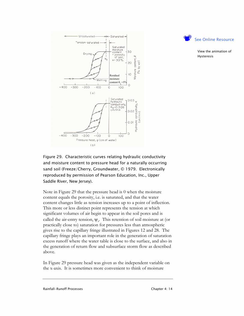
Figure 28. Illustration of capillary rise due to surface tension and relationship between pore size distribution and soil water retention curves. The flow of water in unsaturated porous media is also governed by Darcy's equation. However, since the moisture content and the size of the pores occupied by water reduces as the magnitude of the suction head is increased (becomes more negative), the paths for water to flow become fewer in number, of smaller cross section and more tortuous. All these effects serve to reduce hydraulic conductivity. Figure 29 illustrates the form of the relationships giving the dependence of suction head and hydraulic conductivity on soil moisture content. This issue is further complicated in that it has been observed experimentally that the ψ(θ) relationship is hysteretic; it has a different shape when soils are wetting than when they are drying. This also translates into hysteresis in the relationship between hydraulic conductivity and moisture content. The physical processes responsible for hysteresis are discussed by Bear (1979). The curves illustrating the relationship between ψ, θ and K are referred to as soil water characteristic curves, or soil water retention curves. While hysteresis can have a significant influence on soil-moisture movement, it is difficult to model mathematically and is therefore not commonly incorporated in hydrologic models.


Residual moisture content θr =5%

Figure 29. Characteristic curves relating hydraulic conductivity and moisture content to pressure head for a naturally occurring sand soil (Freeze/Cherry, Groundwater, © 1979. Electronically reproduced by permission of Pearson Education, Inc., Upper Saddle River, New Jersey).

Note in Figure 29 that the pressure head is 0 when the moisture content equals the porosity, i.e. is saturated, and that the water content changes little as tension increases up to a point of inflection. This more or less distinct point represents the tension at which significant volumes of air begin to appear in the soil pores and is called the air-entry tension, ψa. This retention of soil moisture at (or practically close to) saturation for pressures less than atmospheric gives rise to the capillary fringe illustrated in Figures 12 and 28. The capillary fringe plays an important role in the generation of saturation excess runoff where the water table is close to the surface, and also in the generation of return flow and subsurface storm flow as described above.

In Figure 29 pressure head was given as the independent variable on the x-axis. It is sometimes more convenient to think of moisture

See Online Resource

View the animation of Hysteresis


content as the independent variable. Figure 30 gives an example of the soil water characteristic curves with moisture content as the independent variable. This representation has the advantage of avoiding some of the problem of hysteresis, because K(θ) is less hysteretic than K(ψ) (Tindall et al., 1999).

Note also in Figure 29 that as tension head is increased a point is reached where moisture content is no longer reduced. A certain amount of water can not be drained from the soil, even at high tension head, due to being retained in disconnected pores and immobile films. This is called the residual moisture content or in some cases the irreducible moisture content θr. For practical purpose flow only occurs in soil for moisture contents between saturation, n, and the residual water content θr. This range is referred to as the effective porosity θe=n-θr. When considering flow in unsaturated soil, moisture content is sometimes quantified using the effective saturation defined to scale the range from θr to n between 0 and 1.

r

re n

Sθ−θ−θ

= (24)

The soil water characteristic curves are a unique property of each soil, related to the size distribution and structure of the pore space. For a specific soil the soil water characteristic functions can be determined experimentally through drainage experiments. For practical purposes it is convenient to mathematically represent the characteristic functions using equations and a number of empirical equations have been proposed. Three functional forms proposed by Brooks and Corey (1966), Van Genuchten (1980) and Clapp and Hornberger (1978) are listed. There are no fundamental differences between these equations, they are simply convenient mathematical expressions that approximately fit the empirical shape of many soil characteristic functions.


Figure 30. Variation of soil suction head, |ψ|, and hydraulic conductivity, K, with moisture content (from Chow et al., 1988).

Brooks and Corey (1966):

cesate

beae

SK)S(K

S|||)S(|

=

ψ=ψ −

(25)

van Genuchten (1980):

( )2mm/1

e2/1

esate

m1m/1ee

))S1(1(SK)S(K

1S1|)S(|

−−=

−α

=ψ−−

(26)


Clapp and Hornberger (1978) simplifications of Brooks and Corey functions:

c

sat

b

a

nK)(K

n|||)(|

θ

=θ

θ

ψ=θψ−

(27)

In these equations Ksat is the saturated hydraulic conductivity and b, c, α and m are fitting parameters. The parameter b is referred to as the pore size distribution index because the pore size distribution determines relationship between suction and moisture content (Figure 28). The parameter c is referred to as the pore disconnectedness index because unsaturated hydraulic conductivity is related to how disconnected and tortuous flow paths become as moisture content is reduced. There are theoretical models that relate the soil water retention and hydraulic conductivity characteristic curves. Two common such models are due to Burdine (1953) and Mualem (1976). The Burdine (1953) model suggests c≈2b+3 in equations (25) and (27). The more recent Mualem (1976) model suggests c≈2b+2.5. The K(Se) equation due to van Genuchten uses the Mualem theory. The relative merits of these theories are beyond the scope discussed here. The Brooks and Corey (1966) and Clapp and Hornberger (1978) equations apply only for ψ<ψa and assume θ=n for ψ>ψa, while the van Genuchten (1980) equations provide for a smoother representation of the inflection point in the characteristic curve near saturation. Clapp and Hornberger (1978) and Cosby et al (1984) statistically analyzed a large number of soils in the United States to relate soil moisture characteristic parameters to soil texture class. Parameter values that Clapp and Hornberger (1978) obtained are given in table 1. The Clapp and Hornberger simplification (equation 27) neglects the additional parameter of residual moisture "which generally gives a better fit to moisture retention data" (Cosby et al., 1984) but was adopted in their analysis because "the large amount of variability in the available data suggests a simpler representation." When using values from table 1, one should be aware of this considerable within-soil-type variability as reflected in the standard deviations listed in table 1. Figures 31 and 32 show the characteristic curves for soils with different textures using the parameter values from table 1. The USDA-ARS Salinity Laboratory has developed a software program Rosetta that estimates the soil moisture retention function ψ(θ) and hydraulic conductivity


function and K(θ) based upon soil texture class or sand, silt and clay percentages.

Table 1. Clapp and Hornberger (1978) parameters for equation (27) based on analysis of 1845 soils. Values in parentheses are standard deviations.

Soil Texture Porosity n Ksat

(cm/hr) |ψa| (cm) b Sand 0.395 (0.056) 63.36 12.1 (14.3) 4.05 (1.78) Loamy sand 0.410 (0.068) 56.16 9 (12.4) 4.38 (1.47) Sandy loam 0.435 (0.086) 12.49 21.8 (31.0) 4.9 (1.75) Silt loam 0.485 (0.059) 2.59 78.6 (51.2) 5.3 (1.96) Loam 0.451 (0.078) 2.50 47.8 (51.2) 5.39 (1.87) Sandy clay loam 0.420 (0.059) 2.27 29.9 (37.8) 7.12 (2.43) Silty clay loam 0.477 (0.057) 0.612 35.6 (37.8) 7.75 (2.77) Clay loam 0.476 (0.053) 0.882 63 (51.0) 8.52 (3.44) Sandy clay 0.426 (0.057) 0.781 15.3 (17.3) 10.4 (1.64) Silty clay 0.492 (0.064) 0.371 49 (62.0) 10.4 (4.45) Clay 0.482 (0.050) 0.461 40.5 (39.7) 11.4 (3.7)

1.0E+00

1.0E+01

1.0E+02

1.0E+03

1.0E+04

1.0E+05

1.0E+06

1.0E+07

1.0E+08

1.0E+09

1.0E+10

1.0E+11

1.0E+12

1.0E+13

1.0E+14

0 0.2 0.4 0.6 0.8 1

θ/n

|ψ| (

cm)

sandloamy sandsandy loamsilt loamloamsandy clay loamsilty clay loamclay loamsandy claysilty clayclay

Figure 31. Soil suction head, |ψ|, for different soil textures using the Clapp and Hornberger (1978) parameterization (Equation 27).

See Online Resource

Excel spreadsheet with table and Figures in electronic form

See Online Resource

Rosetta soil property program http://www.ussl.ars.usda.gov/models/rosetta/rosetta.HTM


One can infer from the soil moisture retention curves that as moisture drains from soil under gravitational processes, the hydraulic conductivity is reduced and drainage rate reduced. A point is reached where, for practical purposes, downward drainage has materially ceased. The value of water content remaining in a unit volume of soil after downward gravity drainage has materially ceased is defined as field capacity. A difficulty inherent in this definition is that no quantitative specification of what is meant by "materially ceased" is given. Sometimes a definition of drainage for three days following saturation is used. This is adequate for sandy and loamy soils, but is problematic for heavier soils that drain for longer periods.

1.0E-261.0E-241.0E-221.0E-201.0E-181.0E-161.0E-141.0E-121.0E-101.0E-081.0E-061.0E-041.0E-021.0E+001.0E+02

0 0.2 0.4 0.6 0.8 1

θ/n

K( θ

) (cm

/hr)

sandloamy sandsandy loamsilt loamloamsandy clay loamsilty clay loamclay loamsandy claysilty clayclay

Figure 32. Hydraulic conductivity K(θ) for different soil textures using the Clapp and Hornberger (1978) parameterization (Equation 27).

Because of the difficulty associated with precisely when drainage has materially ceased, a practical approach is to define field capacity as the moisture content corresponding to a specific pressure head. Various studies define field capacity as the moisture content corresponding to a pressure head, ψ, in the range -100 cm to -500 cm with a value of -340 cm being quite common (Dingman, 2002) . The difference between moisture content at saturation and field capacity is referred to as drainable porosity, i.e. nd = n-θ(ψ=-100 cm).


The notion of field capacity is similar to the notion of residual moisture content defined earlier; however some equations (e.g. equation 27) do not use residual moisture content. A distinction in the definitions can be drawn in that residual moisture content is a theoretical value below which there is no flow of water in the soil, i.e. hydraulic conductivity is 0, while field capacity is a more empirical quantity practically defined as the moisture content corresponding to a specific negative pressure head.

In nature, water can be removed from a soil that has reached field capacity only by direct evaporation or by plant uptake. Plants cannot exert suctions stronger than about -15000 cm and when the water content is reduced to the point corresponding to that value on the moisture characteristic curve, transpiration ceases and plants wilt. This water content is called the permanent wilting point θpwp. The difference between the field capacity and permanent wilting point is the water available for plant use, called plant available water content, θa = θfc-θpwp. Although most important for irrigation scheduling in agriculture this is relevant for runoff generation processes because during dry spells vegetation may reduce the surface water content to a value between field capacity and permanent wilting point. The antecedent moisture content plays a role in the generation of runoff. Figure 33 shows a classification of water status in soils based on pressure head. Figure 34 shows ranges of porosity, field capacity and wilting point for soils of various textures.

Figure 33. Soil-water status as a function of pressure (tension). Natural soils do not have tensions exceeding about -31000 cm; in this range water is absorbed from the air (Dingman, Physical Hydrology, 2/E, © 2002. Electronically reproduced by permission of Pearson Education, Inc., Upper Saddle River, New Jersey).


Figure 34. Ranges of porosities, field capacities, and permanent wilting points for soils of various textures (Dingman, Physical Hydrology, 2/E, © 2002. Electronically reproduced by permission of Pearson Education, Inc., Upper Saddle River, New Jersey).


References

Bear, J., (1979), Hydraulics of Groundwater, McGraw-Hill, New York, 569 p.

Bras, R. L., (1990), Hydrology, an Introduction to Hydrologic Science, Addison-Wesley, Reading, MA, 643 p.

Brooks, R. H. and A. T. Corey, (1966), "Properties of Porous Media Affecting Fluid Flow," J. Irrig. and Drain. ASCE, 92(IR2): 61-88.

Burdine, N. T., (1953), "Relative Permeability Calculations from Pore Size Distribution Data," Petroleum Transactions AIME, 198: 71-78.

Chow, V. T., D. R. Maidment and L. W. Mays, (1988), Applied Hydrology, McGraw Hill, 572 p.

Clapp, R. B. and G. M. Hornberger, (1978), "Empirical Equations for Some Soil Hydraulic Properties," Water Resources Research, 14: 601-604.

Cosby, B. J., G. M. Hornberger, R. B. Clamp and T. R. Ginn, (1984), "A Statistical Exploration of the Relationships of Soil Moisture Characteristics to the Physical Properties of Soils," Water Resources Research, 20(6): 682-690.

Dingman, S. L., (2002), Physical Hydrology, 2nd Edition, Prentice Hall, 646 p.

Freeze, R. A. and J. A. Cherry, (1979), Groundwater, Prentice Hall, Englewood Cliffs, 604 p.

Hillel, D., (1980), Fundamentals of Soil Physics, Academic Press, New York, NY.

Mualem, Y., (1976), "A New Model for Predicting the Hydraulic Conductivity of Unsaturated Porous Media," Water Resources Research, 12(3): 513-522.

Tindall, J. A., J. R. Kunkel and D. E. Anderson, (1999), Unsaturated Zone Hydrology for Scientists and Engineers, Prentice Hall, Upper Saddle River, New Jersey, 624 p.


Van Genuchten, M. T., (1980), "A Closed Form Equation for Predicting the Hydraulic Conductivity of Unsaturated Soils," Soil Sci. Soc. Am. J., 44: 892-898.

Copyright © 2003 David G Tarboton, Utah State University

Chapter 5 At a Point Infiltration Models

for Calculating Runoff


CHAPTER 5: AT A POINT INFILTRATION MODELS FOR CALCULATING RUNOFF Infiltration is the movement of water into the soil under the driving forces of gravity and capillarity, and limited by viscous forces involved in the flow into soil pores as quantified in terms of permeability or hydraulic conductivity. The infiltration rate, f, is the rate at which this process occurs. The infiltration rate actually experienced in a given soil depends on the amount and distribution of soil moisture and on the availability of water at the surface. There is a maximum rate at which the soil in a given condition can absorb water. This upper limit is called the infiltration capacity, fc. Note that this is a rate, not a depth quantity. It is a limitation on the rate at which water can move into the ground. If surface water input is less than infiltration capacity, the infiltration rate will be equal to the surface water input rate, w. If rainfall intensity exceeds the ability of the soil to absorb moisture, infiltration occurs at the infiltration capacity rate. Therefore to calculate the actual infiltration rate, f, is the lesser of fc or w. Water that does not infiltrate collects on the ground surface and contributes to surface detention or runoff (Figure 35). The surface overland flow runoff rate, R, is the excess surface water input that does not infiltrate.

R = w - f (28)

This is also often referred to as precipitation excess.

The infiltration capacity declines rapidly during the early part of a storm and reaches an approximately constant steady state value after a few hours (Figure 7). The focus of this section on at a point infiltration models for calculating runoff is on how to calculate runoff accounting for the reduction of infiltration capacity. We use accumulated infiltration depth, F, as an independent variable and write infiltration capacity as a decreasing function fc(F), then as F increases with time fc is reduced. fc may be a gradually decreasing function, or a threshold function, as in the case of saturation excess runoff where there is a finite soil moisture deficit that can accommodate surface water input.

Several processes combine to reduce the infiltration capacity. The filling of fine pores with water reduces capillary forces drawing water into pores and fills the storage potential of the soil. Clay swells as it becomes wetter and the size of pores is reduced. The impact of


raindrops breaks up soil aggregates, splashing fine particles over the surface and washing them into pores where they impede the entry of water. Coarse-textured soils such as sands have large pores down which water can easily drain, while the exceedingly fine pores in clays retard drainage. If the soil particles are held together in aggregates by organic matter or a small amount of clay, the soil will have a loose, friable structure that will allow rapid infiltration and drainage.

Figure 35. Surface Runoff occurs when surface water input exceeds infiltration capacity. (a) Infiltration rate = rainfall rate which is less than infiltration capacity. (b) Runoff rate = Rainfall intensity – Infiltration capacity (from Water in Environmental Planning, Dunne and Leopold, 1978)

The depth of the soil profile and its initial moisture content are important determinants of how much infiltrating water can be stored in the soil before saturation is reached. Deep, well-drained, coarse-textured soils with large organic matter content will tend to have high infiltration capacities, whereas shallow soil profiles developed in clays will accept only low rates and volumes of infiltration.

Vegetation cover and land use are very important controls of infiltration. Vegetation and litter protect soil from packing by raindrops and provide organic matter for binding soil particles together in open aggregates. Soil fauna that live on the organic matter assist this process by churning together the mineral particles and the organic material. The manipulation of vegetation during land use causes large differences in infiltration capacity. In particular, the stripping of forests and their replacement by crops that do not cover the ground efficiently and do not maintain a high organic content in the soil often lower the infiltration capacity drastically. Soil surfaces trampled by livestock or compacted by vehicles also have reduced


infiltration capacity. The most extreme reduction of infiltration capacity, of course, involves the replacement of vegetation by an asphalt or concrete cover in urban areas. In large rainstorms it is the final, steady state rate of infiltration that largely determines the amount of surface runoff that is generated.

The calculation of infiltration at a point combines the physical conservation of mass (water) principle expressed through the continuity equation with quantification of unsaturated flow through soils, expressed by Darcy's equation. Here we will derive the continuity equation then substitute in Darcy's equation to obtain as a result Richard's equation which describes the vertical movement of water through unsaturated soil. Figure 36 shows a control volume in an unsaturated porous medium. Consider flow only in the vertical direction. The specific discharge across the bottom surface into the volume is denoted as q, and the outflow across the top surface is denoted as q+∆q. The volumetric flux is specific discharge times cross sectional area, yxA ∆⋅∆= . The volume of water in the control volume is the moisture content times the total volume (equation 7), here zyxV ∆⋅∆⋅∆= . Therefore we can write

Change in Storage = (Inflow rate – Outflow rate) x (time interval) ∆θ ∆x ∆y ∆z = (q ∆x ∆y – (q+∆q) ∆x ∆y) ∆t (29)

Dividing by ∆x ∆y ∆z ∆t and simplifying results in

zq

t ∆∆

−=∆

θ∆ (30)

Now letting ∆z and ∆t get smaller and approach 0, as is usual in calculus, we get

zq

t ∂∂

−=∂θ∂ (31)

This is the continuity equation in one direction (the vertical direction z). In a more general case where flow can be three dimensional, the continuity equation is obtained in a similar fashion as

qzq

yq

xq

tzyx •−∇=

∂∂

+∂∂

+∂∂

−=∂θ∂ (32)


where the operator ∇ is used as shorthand notation for

∂∂

∂∂

∂∂

z,

y,

x and q denotes the specific discharge vector (qx, qy, qz)

with component in each coordinate direction.

Figure 36. Control volume for development of the continuity equation in an unsaturated porous medium (from Chow et al., 1988).

Substituting Darcy's equation (16) into (31) gives

zhK

zt ∂∂

∂∂

=∂θ∂ (33)

In this equation h = ψ+z (equation 18) resulting in

+

∂ψ∂

∂∂

=∂θ∂ K

zK

zt (34)

This equation is known as Richard's equation and it describes the vertical movement of water through unsaturated soil. Although simple appearing, its solution is complicated by the soil moisture characteristic relationships relating moisture content and pressure head θ(ψ) and Hydraulic conductivity and pressure head or moisture content K(ψ) or K(θ) discussed above (equations 25, 26, 27 and Figures 29-32). Richard's equation may be written in one of two forms depending on whether we take moisture content, θ, or pressure head, ψ, as the independent variable.


In terms of moisture content, Richard's equation is written

θ+

∂θ∂

θ∂∂

=

θ+

∂θ∂

θψ

θ∂∂

=

θ+

∂θψ∂

θ∂∂

=∂θ∂

)(Kz

)(Dz

)(Kzd

d)(Kz

)(Kz

)()(Kzt

(35)

In this equation the explicit functional dependence on moisture

content, θ, has been shown. The quantity D(θ)=θψ

θdd)(K is called

the soil water diffusivity, because the term involving it is similar to a diffusion term in the diffusion equation. For specific parameterizations of the soil moisture characteristic curves ψ(θ) and K(θ), such as equations (25-27), D(θ) can be derived.

In terms of pressure head, Richard's equation is written

ψ+

∂ψ∂

ψ∂∂

=∂ψ∂

ψ

ψ+

∂ψ∂

ψ∂∂

=∂ψ∂

ψθ

=∂

ψθ∂

)(Kz

)(Kzt

)(C

)(Kz

)(Kztd

dt

)(

(36)

As above, in this equation the explicit functional dependence on pressure head, ψ, has been shown. The quantity C(ψ) = dθ/dψ is called the specific moisture capacity.

Analytic solutions for Richard's equation are known for specific parameterizations of the functions K(θ) and D(θ) or K(ψ) and C(ψ) and for specific boundary conditions (see e.g. Philip, 1969; Parlange et al., 1999; Smith et al., 2002). There are also computer codes that implement numerical solutions to Richard's equation. Hydrus 1-D is one such code available from the USDA-ARS Salinity Laboratory (http://www.ussl.ars.usda.gov/models/hydr1d1.HTM) Computational codes based on the moisture content form tend to be better at conserving moisture and dealing with dryer soil conditions. These have problems as saturation is increased because moisture content becomes capped at the porosity and dψ/dθ tends to infinity. Computational codes based on the pressure head form are able to


better handle the transition between saturated and unsaturated flow near the water table, but because moisture content is not a specific state variable in their solution, are not as good at conserving mass. Pressure head (and suction) is a continuous function of depth, however in layered soils moisture content is discontinuous at the interface between layers where hydraulic conductivity changes. Computer codes using ψ as the independent variable cope better with these discontinuities. Some approaches to the numerical solution of Richard's equation combine the moisture content and pressure head representations (Celia et al., 1990).

Although Richard's equation is fundamental to the movement of water through unsaturated soil we do not give numerical solutions here, because these are complex and require detailed soils data that are usually not available. Instead we analyze the development of soil moisture versus depth profiles more qualitatively to develop the empirical models used to calculate infiltration.

Consider a block of soil that is homogeneous with water table at depth and initially hydrostatic conditions above the water table (Figure 37). Hydrostatic conditions mean that water is not moving, so in Darcy's equation (16), q=0, dh/dz=0 and therefore the hydraulic head h is constant. Because pressure head ψ is 0 at the water table equation (18) implies that ψ = -z where z is the height above the water table. This gives initial moisture content at each depth z

θ(z) = θ(ψ= -z) (37)

from the soil moisture retention characteristic.

Beginning at time t=0, liquid water begins arriving at the surface at a specified surface water input rate w. This water goes into storage in the layer, increasing its water content. The increase in water content causes an increase in hydraulic conductivity according to the hydraulic conductivity – water content relation for the soil (equations 25, 26, 27). Also because the water content is increased, the absolute value of the negative pressure head is reduced according to the soil moisture characteristic and a downward hydraulic gradient is induced. This results in a flux out of the surface layer in to the next layer down. This process happens successively in each layer as water input continues, resulting in the successive water content profiles at times t1, t2 and t3 shown in Figure 37.


(a)

(b)(c)

Figure 37. Infiltration excess runoff generation mechanism. (a) Moisture content versus depth profiles and (b) Runoff generation time series. (Bras, Hydrology: An introduction to Hydrologic Science, © 1990. Electronically reproduced by permission of Pearson Education, Inc., Upper Saddle River, New Jersey) (c) Wetting front in a sandy soil exposed after intense rain (Dingman, Physical Hydrology, 2/E, © 2002. Electronically reproduced by permission of Pearson Education, Inc., Upper Saddle River, New Jersey).

Note that the downward hydraulic gradient inducing infiltration is from a combination of the effect of gravity, quantified by the elevation head, and capillary surface tension forces, quantified by the pressure head (negative due to suction) being lower at depth due to lower moisture content. Now if water input rate is greater than the saturated hydraulic conductivity (i.e. w > Ksat), at some point in time the water content at the surface will reach saturation. At this time the infiltration capacity drops below the surface water input rate and runoff is generated. This is indicated in Figure 37 as time t3 and is called the ponding time. After ponding occurs, water continues to infiltrate and a zone of saturation begins to propagate downward into the soil, as show for t4 in Figure 37. This wave of soil moisture propagating into the soil (from t1 to t4) is referred to as a wetting front. After ponding the infiltration rate is less than the water input


rate and the excess water accumulates at the surface and becomes infiltration excess runoff. As time progresses and the depth of the zone of saturation increases, the contribution of the suction head to the gradient inducing infiltration is reduced, so infiltration capacity is reduced.

The time series of water input, infiltration and surface runoff during this process is depicted in Figure 37b, which shows a reduction in infiltration with time and a corresponding increase in runoff. The necessary conditions for the generation of runoff by the infiltration excess mechanism are (1) a water input rate greater than the saturated hydraulic conductivity of the soil, and (2) a surface water input duration longer than the required ponding time for a given initial soil moisture profile and water input rate.

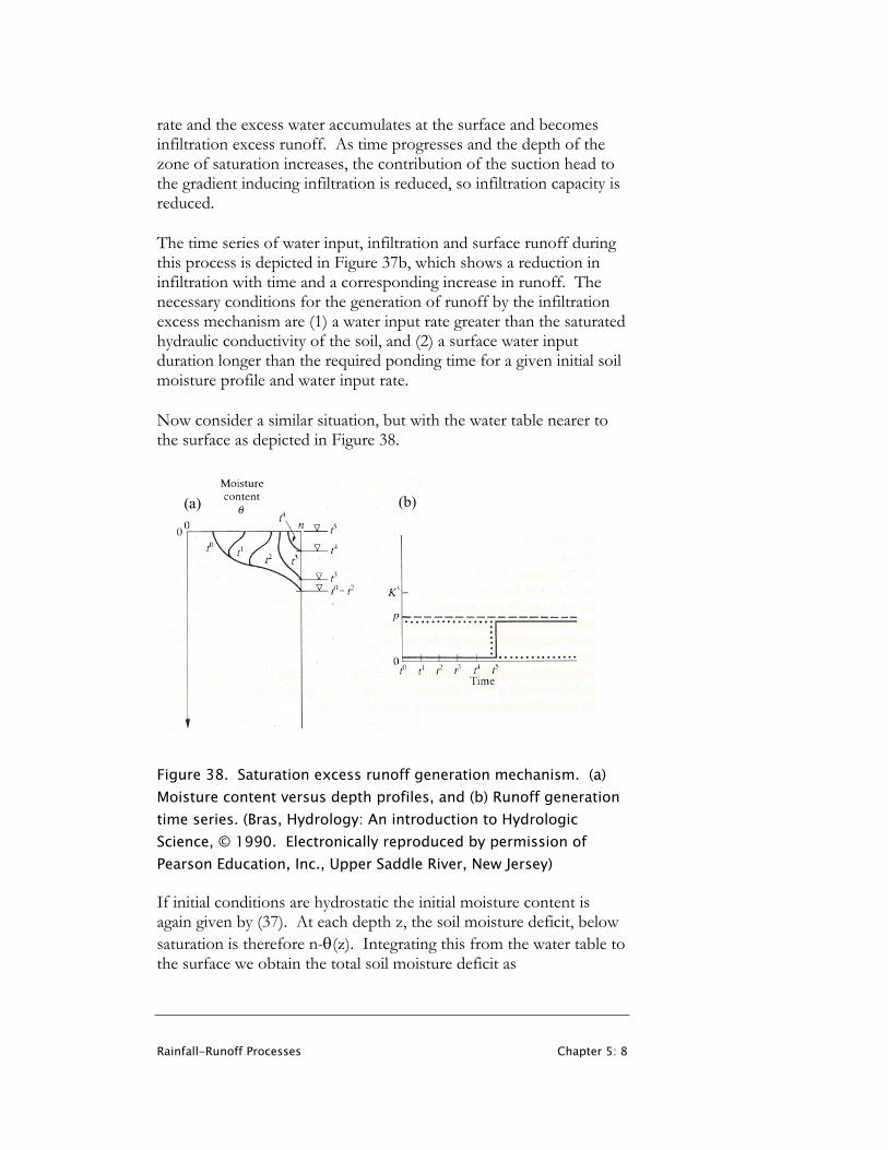
Now consider a similar situation, but with the water table nearer to the surface as depicted in Figure 38.

(a) (b)

Figure 38. Saturation excess runoff generation mechanism. (a) Moisture content versus depth profiles, and (b) Runoff generation time series. (Bras, Hydrology: An introduction to Hydrologic Science, © 1990. Electronically reproduced by permission of Pearson Education, Inc., Upper Saddle River, New Jersey)

If initial conditions are hydrostatic the initial moisture content is again given by (37). At each depth z, the soil moisture deficit, below saturation is therefore n-θ(z). Integrating this from the water table to the surface we obtain the total soil moisture deficit as


∫ θ−=wz

0

dz))z(n(D (38)

This defines the total amount of water that can infiltrate into a soil profile. Surface water input to a situation like this again (similar to the infiltration excess case) results in soil moisture profiles at times t1, t2, t3, and t4, depicted in Figure 38a. However, even if w < Ksat, a point in time is reached where the accumulated surface water input is equal to D. At this time the soil profile is completely saturated and no further water can infiltrate. Infiltration capacity goes to zero, and all surface water input becomes runoff. This is the saturation excess runoff generation mechanism. The time series of surface water input, infiltration and surface runoff for this mechanism are depicted in Figure 38b.

Note that the infiltration excess and saturation excess mechanisms are not mutually exclusive. One or the other could occur in a given situation given different initial depths to the water table and surface water input rates.

Green-Ampt Model

The Green – Ampt (1911) model is an approximation to the infiltration excess process described above and depicted in Figure 37. In Figure 37 successive soil moisture profiles were shown as curves, with moisture content gradually reducing to the initial conditions below the wetting front. The Green – Ampt model approximates the curved soil moisture profiles, that result in practice, and from solution to Richard's equation, as a sharp interface with saturation conditions, θ=n, above the wetting front and initial moisture content, θ=θo, below the wetting front (Figure 39). The initial moisture content is assumed to be uniform over depth. Let L denote the depth to the wetting front. Denote the difference between initial and saturation moisture contents as ∆θ = n - θo. Then the depth of infiltrated water following initiation of infiltration is

F=L ∆θ (39)

The datum for the definition of hydraulic head is taken as the surface and an unlimited supply of surface water input is assumed, but with small ponding depth, so the contribution to hydraulic gradient from the depth of ponding at the surface is neglected. Immediately below


the wetting front, at depth just greater than L, the soil is at its initial unsaturated condition, with corresponding suction head |ψf|. The hydraulic head difference driving infiltration, measured from the surface to just below the wetting front is therefore

h=-(L + |ψf|) (40)

The hydraulic gradient is obtained by dividing this head difference by the distance L between the surface and the wetting front to obtain

L||L

dzdh fψ+

−= (41)

Moisture content, θ0.50.40.30.20.1

Dep

th, z

, (cm

)

10

20

30

40

t1

t2t3

t4

L

∆θ

Initial moisture content θoSaturation moisture content θs equivalent to porosity, n

Figure 39. Green-Ampt model idealization of wetting front penetration into a soil profile.

Using this in Darcy's equation (16) gives the infiltration capacity as


+=

θ∆ψ

+=

ψ

+=ψ+

=

FP1K

F||1K

L||1K

L||LKf

satf

sat

fsat

fsatc

(42)

where in the third expression (39) has been used to express L=F/ θ∆ . This provides an expression for the reduction in infiltration capacity as a function of infiltrated depth fc(F). The parameters involved are Ksat and the product P= θ∆ψ || f . Using the soil moisture characteristic ψf may be estimated as

)( of θψ=ψ (43)

Values for θo may be estimated from field capacity θfc, or wilting point θpwp, depending on the antecedent conditions. Rawls et al. (1993) recommended evaluating || fψ from the air entry pressure as

||6b23b2|| af ψ

++

=ψ (44)

where || aψ and b are from table 1. The latter simpler approach appears to be justified for most hydrologic purposes (Dingman, 2002). Table 2 gives Green-Ampt infiltration parameters for soil texture classes reported by Rawls et al. (1983).

Given a surface water input rate of w, the cumulative infiltration prior to ponding is F = wt. Ponding occurs when infiltration capacity decreases to the point where it equals the water input rate, fc=w. Setting fc=w in (42) and solving for F one obtains the cumulative infiltration at ponding

Green-Ampt cumulative infiltration at ponding:

)Kw(||KFsat

fsatp −

θ∆ψ= (45)

The time to ponding is then

Green-Ampt time to ponding:

tp=Fp/w)Kw(w

||K

sat

fsat

−θ∆ψ

= (46)


Table 2. Green – Ampt infiltration parameters for various soil classes (Rawls et al., 1983). The numbers in parentheses are one standard deviation around the parameter value given.

Soil Texture

Porosity n Effective porosity θe

Wetting front soil suction

head |ψf| (cm)

Hydraulic conductivity Ksat (cm/hr)

Sand 0.437 (0.374-0.500)

0.417 (0.354-0.480)

4.95 (0.97-25.36)

11.78

Loamy sand

0.437 (0.363-0.506)

0.401 (0.329-0.473)

6.13 (1.35-27.94)

2.99

Sandy loam

0.453 (0.351-0.555)

0.412 (0.283-0.541)

11.01 (2.67-45.47)

1.09

Loam 0.463 (0.375-0.551)

0.434 (0.334-0.534)

8.89 (1.33-59.38)

0.34

Silt loam 0.501 (0.420-0.582)

0.486 (0.394-0.578)

16.68 (2.92-95.39)

0.65

Sandy clay loam

0.398 (0.332-0.464)

0.330 (0.235-0.425)

21.85 (4.42-108.0)

0.15

Clay loam 0.464 (0.409-0.519)

0.309 (0.279-0.501)

20.88 (4.79-91.10)

0.1

Silty clay loam

0.471 (0.418-0.524)

0.432 (0.347-0.517)

27.30 (5.67-

131.50)

0.1

Sandy clay 0.430 (0.370-0.490)

0.321 (0.207-0.435)

23.90 (4.08-140.2)

0.06

Silty clay 0.479 (0.425-0.533)

0.423 (0.334-0.512)

29.22 (6.13-139.4)

0.05

Clay 0.475 (0.427-0.523)

0.385 (0.269-0.501)

31.63 (6.39-156.5)

0.03

To solve for the infiltration that occurs after ponding with the Green Ampt model, recognize that infiltration rate is the derivative of cumulative infiltration, and is limited by the infiltration capacity

f(t) )t(fdtdF

c== (47)

Here the functional dependence on time is explicitly shown. Now using (42) the following differential equation is obtained

See Online Resource

Excel spreadsheet with table in electronic form


)FP1(K

dtdF

sat += (48)

Using separation of variables this can be integrated from any initial cumulative infiltration depth Fs at time ts to a final cumulative infiltration depth F at time t

Green-Ampt infiltration under ponded conditions:

++

+−

=−PFPFln

KP

KFFtt s

satsat

ss (49)

There is no explicit expression for F from this equation. However by setting ts = tp, and Fs = Fp this equation can be solved numerically for F given any arbitrary t (greater than tp) to give the cumulative infiltration as a function of time.

An important concept that emerges from the Green – Ampt model is that infiltration capacity during a storm decreases as a function of cumulative infiltrated depth. This provides for a decrease in infiltration capacity and increase in runoff ratio with time, consistent with empirical observations. The dependence on cumulative infiltrated depth means that cumulative infiltrated depth may be treated as a state variable and that variable rainfall rates, and hence variable infiltration rates, and consequent variability in the rate at which infiltration capacity is reduced, is modeled quite naturally using the Green – Ampt model. This is referred to as the infiltrability-depth approximation (IDA) (Smith et al., 2002).

In the Horton and Philip infiltration models discussed below the decrease in infiltration capacity is modeled explicitly as a function of time rather than cumulative infiltrated depth. Alternative equivalent solution procedures can be developed using the time compression approach (Mein and Larson, 1973) or the infiltrability-depth approximation. Here the infiltrability-depth approximation is used, because this provides a more natural and physically sound basis for understanding and using this approach.

Horton Model

The Horton infiltration capacity formulation (Horton, 1939; although apparently first proposed by others Gardner and Widstoe, 1921) has an initial infiltration capacity value f0, for dry or pre-storm conditions. Once surface water input and infiltration commences,


this decreases in an exponential fashion to a steady state infiltration capacity, f1.

kt101c e)ff(f)t(f −−+= (50)

Here k is a rate parameter quantifying the rate at which infiltration capacity decreases with time. Eagleson (1970) showed that Horton's equation can be derived from Richard's equation by assuming that K and D are constants independent of the moisture content of the soil. Under these conditions equation (35) reduces to

2

2

zD

t ∂θ∂

=∂θ∂ (51)

which is the standard form of a diffusion equation and may be solved to yield the moisture content as a function of time and depth. Horton's equation results from solving for the rate of moisture diffusion at the soil surface under specific initial and boundary conditions.

Figure 40 shows the Horton infiltration equation as applied to a given rainfall event. It may be argued that at point t1 where surface water input rate first exceeds infiltration capacity; the actual infiltration capacity will be larger than that given by fc(t1) in the Figure. This is because fc(t1) assumes that the infiltration rate has decayed from f0 due to increased soil moisture from the water that has infiltrated. The cumulative depth of infiltration that has contributed to soil moisture is given by the area under the fc(t) curve between time 0 and t1. This is less than the maximum that would have infiltrated were the surface saturated with an unlimited supply of moisture. To account for this discrepancy, the time compression approach (Mein and Larson, 1973) illustrated in Figure 40, was developed. This can be viewed as a shifting of the fc(t) curve to the right, but is more fundamentally a recasting of equation (50) in terms of cumulative infiltrated depth, F, rather than t, using the infiltrability-depth approximation. Under conditions of unlimited surface water input, the cumulative infiltration up to time t is expressed as

)e1(k

)ff(tfdt)t(fF kt101

t

0c

−−−

+== ∫ (52)


Now eliminating t between equation (50) and (52) (by solving (50) for t and substituting in (52)) results in

−−

−−

=10

1c1c0

ffffln

kf

kffF (53)

This is an implicit equation that, given F, can be solved for fc, i.e. it is an implicit function fc(F).

f0

f1

kt101c e)ff(f)t(f −−+=

t1toF1

t0

)tt(k10

1ocoe)ff(

f)tt(f−−−

+=−

Figure 40. Partition of surface water input into infiltration and runoff using the Horton infiltration equation. Ponding starts at t1. The cumulative depth of water that has infiltrated up to this time is the area F1 (shaded gray). This is less than the maximum possible infiltration up to t1 under the fc(t) curve. To accommodate this the fc(t) curve is shifted in time by an amount to so that the cumulative infiltration from to to t1 (hatched area) equals F1. Runoff is precipitation in excess of fc(t-to) (blue area). Given a surface water input rate of w, the cumulative infiltration prior to ponding is F = wt. Ponding occurs when infiltration capacity decreases to the point where it equals the water input rate, fc=w. Setting fc=w in (53) one obtains the cumulative infiltration at ponding


Horton cumulative infiltration at ponding:

−−

−−

=10

110p ff

fwlnkf

kwfF (54)


Horton time to ponding:

tp=Fp/w

−−

−−

=10

110

fffwln

kwf

kwwf (55)

To solve for the infiltration that occurs after ponding with the Horton model, recognize that infiltration rate under ponded conditions is given by fc, but with the time origin shifted so that the cumulative infiltration F (equation 52) matches the initial cumulative infiltration Fs at an initial time ts. From (52) to is solved implicitly in

)e1(k

)ff()tt(fF )tt(k100s1s

0s −−−−

+−= (56)

Then cumulative infiltration F at any time t (t>ts) can be obtained from

Horton infiltration under ponded conditions:

)e1(k

)ff()tt(fF )tt(k1001

0−−−−

+−= (57)

Philip Model

Philip (1957; 1969) solved Richard's equation under less restrictive conditions (than used by Eagleson (1970) to obtain Horton's equation) by assuming that K and D can vary with the moisture content θ. Philip employed the Boltzmann transformation

−1/2 = θ zt)B( to convert (35) into an ordinary differential equation in B, and solved this equation to yield an infinite series for cumulative infiltration F(t). Approximating the solution by retaining only the first two terms in the infinite series results in

F(t) = Sp t1/2 + Kp t (58)


where Sp is a parameter called sorptivity, which is a function of the soil suction potential and Kp is a hydraulic conductivity. Differentiating with respect to time t, we get

K tS 21 (t)f p

1/2-pc += (59)

As time increases the first term will decrease to 0 in the limit and fc(t) will converge to Kp. →∞, fc(t) tends to Kp. The two terms in Philip's equation represent the effects of soil suction head and gravity head respectively. As with Horton's equation, this equation can also be recast, using the infiltrability-depth approximation, in terms of cumulative infiltrated depth, F, rather than t, by eliminating t between equations (58) and (59).

pp2p

pppc

SFK4S

SKK(F) f

−++= (60)

In Philip's equation Sp is theoretically related to the wetting front suction (and hence to the initial water content of the soil) and to Ksat, and Kp is related to Ksat. Rawls et al. (1993; citing Youngs, 1964) suggested that Sp is given by

2/1fsatp |)|K2(S ψθ∆= (61)

with |ψf| from (43) or (44) and ∆θ=n-θo, the difference between porosity and initial moisture content. Rawls et al. (1993; citing Youngs, 1964) reports Kp ranging from Ksat/3 to Ksat with Ksat the preferred value. Kp=Ksat is consistent with the reasoning of the Green – Ampt approach and true for an asymptotic infiltration capacity. However Dingman (2002; citing Sharma et al., 1980) reports that for short time periods smaller values of Kp, generally in the range between 1/3 and 2/3 of Ksat better fit measured values.

As for the Horton model, given a surface water input rate of w, the cumulative infiltration prior to ponding is F = wt. Ponding occurs when infiltration capacity decreases to the point where it equals the water input rate, i.e. fc=w. Setting fc=w in (60) one obtains the cumulative infiltration at ponding


Philip cumulative infiltration at ponding:

2p

p2p

p )Kw(2)2/Kw(S

F−−

= (62)


Philip time to ponding:

tp=Fp/w 2p

p2p

)Kw(w2)2/Kw(S

−−

= (63)

Again, as for the Horton model, to solve for the infiltration that occurs after ponding, recognize that infiltration rate under ponded conditions is given by fc, but with the time origin shifted so that the cumulative infiltration F (equation 58) matches the initial cumulative infiltration Fs at an initial time ts. From (58) to is solved to be

( )2psp2p2

ps0 SFK4S

K41tt −+−= (64)

Then cumulative infiltration F at any time t (t>ts) can be obtained from

Philip infiltration under ponded conditions: )tt(K)tt(SF 0p

2/10p −+−= (65)

Working with at a point infiltration models

In many practical applications the parameters in the Green – Ampt model (Ksat and P), Horton model (f0, f1 and k) and Philip model (Sp and Kp) are treated simply as empirical parameters whose values are those that best fit infiltration data, or as fitting parameters in relating measured rainfall to measured runoff. The equations (42), (53) and (60) provide different, somewhat physical, somewhat empirical representations of the tendency for infiltration capacity to be reduced in response to the cumulative infiltrated depth.

The functions fc(F) derived above provide the basis for the calculation of runoff at a point, given a time series of surface water inputs, and the soil conditions, quantified in terms of infiltration model parameters. The problem considered is: Given a surface water input hyetograph, and the parameters of an infiltration


equation, determine the ponding time, the infiltration after ponding occurs, and the runoff generated. The process is illustrated in Figure 41. A discrete representation is used for the surface water input using the time average surface water input in each time interval as input to the calculations. This is the typical way that a precipitation hyetograph is represented. There is flexibility to have the time interval as small as required to represent more detail in the input and output. The output is the runoff generated from excess surface water input over the infiltration capacity integrated over each time interval. Infiltration capacity decreases with time due to its dependence on the cumulative infiltrated depth F, which serves as a state variable through the calculations.

Time

Surface Water InputInfiltration Capacity

RunoffRunoff

Figure 41. Pulse runoff hyetograph obtained from surface water input hyetograph and variable infiltration capacity. Figure 42 presents a flow chart for determining infiltration and runoff generated under variable surface water input intensity. Consider a series of time intervals of length ∆t. Interval 1 is designated as the interval from t=0 to t=∆t, interval 2 from t=∆t to t=2∆t and so on. In general interval i is from t=(i-1)∆t to t=i∆t. The surface water input intensity during the interval is denoted wt and is taken as constant throughout the interval. The cumulative infiltration depth at the beginning of the interval, representing the initial state, is designated as Ft. The infiltration capacity at the beginning of the interval is then obtained from one of equations (42, 53, 60), corresponding to the Green-Ampt, Horton or Philip models as fc(Ft). The goal is to, given the infiltrated depth, Ft, at the beginning of a time interval and water input, wt, during the interval, calculate infiltration ft during the interval and hence Ft+∆t at the end of the interval, together with any runoff rt generated during the time interval. The calculation is initialized with F0 at the beginning of a storm and proceeds from step to step for the full duration of the


surface water input hyetograph. There are three cases to be considered: (1) ponding occurs throughout the interval; (2) there is no ponding throughout the interval; and (3) ponding begins part-way through the interval. The infiltration capacity is always decreasing or constant with time, so once ponding is established under a given surface water input intensity, it will continue. Ponding cannot cease in the middle of an interval. However ponding may cease at the end of an interval when the surface water input intensity changes. The equations used, based on those derived above, are summarized table 3.

The three infiltration models presented are three of the most popular from a number of at a point infiltration models used in hydrology. Fundamentally there are no advantages of one over the other. The Green-Ampt model provides a precise solution to a relatively crude approximation of infiltration in terms of a sharp wetting front. The Horton model can be justified as a solution to Richard's equation under specific (and practically limiting) assumptions. The Philip model has less limiting assumptions (than Horton) but is a series approximation solution to Richard's equation. Infiltration is a complex process subject to the vagaries of heterogeneity in the soil and preferential flow (as illustrated in Figure 5). Practically, infiltration capacity has the general tendency to decrease with the cumulative depth of infiltrated water and these models provide convenient empirical, but to some extent justifiable in terms of the physical processes involved, equations to parameterize this tendency. The choice of which model to use in any particular setting often amounts to a matter of personal preference and experience and may be based on which one fits the data best, or for which one parameters can be obtained. The Green-Ampt model is popular because Green-Ampt parameters based upon readily available soil texture information has been published (table 2 Rawls et al., 1983). Certain infiltration capacity instruments (Guelph permeameter) have been designed to report their results in terms of parameters for the Philip model.

Three examples, one for each of the models are given to illustrate the procedures involved in calculating runoff using these models. These examples all use the same rainfall input and are designed to produce roughly the same output so that differences between the models can be compared. The examples follow the procedure given in the flow chart (Figure 42) and use the equations summarized in table 3 that were derived above.


Initialize: at t = 0, F t = 0

Is fc

≤ wt

fc> wtf c ≤ w t

No ponding at the beginning of the interval. Calculate tentative values

and column 1.

t w F F t t'

tt ∆ + = ∆+'

tt'c Fromff ∆+

t ' c w f Is ≤

Ponding occurs throughout interval: F t+ ∆ t calculated using infiltration under ponded conditions equations with t

s=t

and F s = F t . Column 3.

t'c wf > t

'c wf ≤

Ponding starts during the interval. Solve for Fp

from wt, column 2.

∆ t ' = ( F p - F t )/w t F t+ ∆ t calculated using infiltration under ponded conditions equationswith t s = t+ ∆ t ' and F s = F p . Column 3.

No ponding throughout interval

' tttt FF ∆+ ∆+ =

Increment time t= t+∆ t

Calculate infiltration capacity fcfrom F t, column 1 of table.

A

CB

D E

Infiltration is f t = Ft+∆t -Ft

Runoff generated is rt= w

t∆ t - f

t

F

G

Figure 42. Flow chart for determining infiltration and runoff generated under variable surface water input intensity.


Table 3. Equations for variable surface water input intensity infiltration calculation.

Infiltration capacity Cumulative infiltration at ponding

Cumulative infiltration under ponded conditions

Green-Ampt

Parameters Ksat and P

+=

FP1satKcf

)satKw(PsatK

pF−

=

w > Ksat

++

+−

=−PFPsFln

satKP

satKsFF

stt

Solve implicitly for F

Horton

Parameters k, fo, f1.

−−

−−

=1fof1fcf

lnk1f

kcfof

F

Solve implicitly for fc given F

−−

−−

=1fof1fw

lnk1f

kwof

pF

fc< w <fo

Solve first for time offset to in

))tt(ke1(k

)1fof()otst(1fsF os −−−

−+−=

then

))tt(ke1(k

)1fof()ott(1fF o−−−

−+−=

Philip

Parameters Kp and Sp

pSFpK42pS

pSpKpK(F) cf

−++=

2)pKw(2

)2/pKw(2pS

pF−

−=

w > Kp

Solve first for time offset to in

2pSsFpK42

pS2pK4

1stot

−+−=

then

)ott(pK2/1)ott(pSF −+−=


Empirical and index methods

The Horton, Philip and Green-Ampt at a point infiltration models attempt to represent the physics of the infiltration process described by Richard's equation, albeit in a simplified way (although given the examples above it may not seem so simple). In many situations the data does not exist to support application of one of these approaches, or spatial variability over a watershed makes this impractical. Empirical and index methods are therefore still rather commonly used in practice, despite being lacking in theoretical basis.

The φ Index. The φ index method requires that a rainfall hyetograph and streamflow hydrograph are available. First baseflow needs to be separated from streamflow to produce the direct runoff hydrograph. Various methods for baseflow separation are illustrated in Figure 46. These are acknowledged as empirical and somewhat arbitrary. The φ index is that constant rate of abstractions (in/h or cm/h) that will yield an excess rainfall hyetograph (ERH) with a total depth equal to the depth of direct runoff over the watershed. The volume of loss is distributed uniformly across the storm pattern as shown in Figure 47. The φ index determined from a single storm is not generally applicable to other storms, and unless it is correlated with basin parameters other than runoff, it is of little value (Viessman et al., 1989).


Figure 46. Baseflow Separation Techniques (from Chow et al, 1988). Linsley et al. (1982) suggest as a rule of thumb N=0.2A, for A in square miles and N in days for the fixed base method (b).

φ index

Figure 47. Representation of a φ index. Runoff Coefficients. Abstractions may also be accounted for by means of runoff coefficients. The most common definition of a runoff coefficient is that it is the ratio of the peak rate of direct runoff to the average intensity of rainfall in a storm. Because of


highly variable rainfall intensity, this value is difficult to determine from observed data. A runoff coefficient can also be defined to be the ratio of runoff to rainfall over a given time period. These coefficients are most commonly applied to storm rainfall and runoff, but can also be used for monthly or annual rainfall and streamflow data.

The SCS Method. The following description follows Chow et al. (1988). The Soil Conservation Service (1972) developed a method for computing abstractions from storm rainfall. For the storm as a whole, the depth of excess precipitation or direct runoff R is always less than or equal to the depth of precipitation P; likewise, after runoff begins, the additional depth of water retained in the watershed, Fa, is less than or equal to some potential maximum retention S. There is some amount of rainfall Ia (initial abstraction) for which no runoff will occur, so the potential runoff is P-Ia. The hypothesis of the SCS method is that the ratios of the two actual to the two potential quantities are equal, that is,

a

aIP

RSF

−= (66)

From the continuity principle

P = R + Ia + Fa (67)

Combining (66) and (67) to solve for R gives

SIP)IP(R

a

2a+−

−= (68)

which is the basic equation for computing the depth of excess rainfall or direct runoff from a storm by the SCS method.

By study of results from many small experimental watersheds, an empirical relation was developed

Ia = 0.2 S (69)


On this basis

S8.0P)S2.0P(R2

+−

= (70)

Plotting data for P and R from many watersheds, the SCS found curves of the type shown in Figure 48. To standardize these curves, a dimensionless curve number CN is defined such that 0≤CN≤100. For impervious and water surfaces CN = 100; for natural surfaces CN < 100.

0123456789

10

0 2 4 6 8 10 12

Precipitation (in)

Dire

ct R

unof

f (in

)

CN=10090 80

70605040

3020

S8.0P)S2.0P(R

2

+−

=

10CN

1000S −=

Figure 48. Solution to the SCS runoff equations.

The curve number and S are related by

10CN

1000S −= (71)

where S is in inches. The curve numbers shown in Figure 48 apply for normal antecedent moisture conditions (AMC II).


For dry conditions (AMC I) or wet conditions (AMC III), equivalent curve numbers can be computed by

)II(CN058.010)II(CN2.4)I(CN

−= (72)

and

)II(CN13.010)II(CN23)III(CN

+= (73)

The range of antecedent moisture conditions for each class is shown in table 7. Curve numbers have been tabulated by the Soil Conservation Service on the basis of soil type and land use. Four soil groups are used:

Group A: Low runoff potential. Soils having high infiltration capacity even if thoroughly wetted, such as deep sand, deep loess, aggregated silts.

Group B: Soils having moderate infiltration capacity if thoroughly wetted, such as shallow loess, aggregated silts.

Group C: Soils having low infiltration capacity if thoroughly wetted, such as clay loams, shallow sandy loam, soils low in organic content and soils usually high in clay.

Group D: High runoff potential. Soils having very low infiltration capacity if thoroughly wetted consisting chiefly of soils that swell significantly when wet, heavy plastic clays, and certain saline soils.

The values of CN for various land uses on these soil types are given in table 8. For a watershed made up of several soil types and land uses a composite average CN is customarily used, despite the nonlinearity of (71) and (70). The SCS curve number methods are empirical and limited in their physical basis, but are often used in practice due to the availability of CN values in soils maps and databases such as STATSGO (USDA-NRCS Soil Survey Division).


Table 7. Classification of antecedent moisture classes (AMC) for the SCS method of rainfall abstraction.

AMC group Dormant Season Growing SeasonI Less than 0.5 Less than 1.4II 0.5 to 1.1 1.4 to 2.1III Over 1.1 Over 2.1

Total 5-day antecedent rainfall (in)

Table 8. Runoff curve numbers for selected agricultural, suburban and urban land uses.

A B C D72 81 88 9962 71 787 8168 79 86 8939 61 74 8030 58 71 7845 66 77 8325 55 70 77

39 61 74 8049 69 79 8489 92 94 9581 88 91 93

Average lot size Average % impervious1/8 acre or less 65 77 85 90 921/4 acre 38 61 75 83 871/3 acre 30 57 72 81 871/2 acre 25 54 70 80 851 acre 20 51 68 79 84Paved parking lots, roofs, driveways, etc. 98 98 98 98Streets and roads: paved with curbs and storm sewers 98 98 98 98 gravel 76 85 89 91 dirt 72 82 87 89

good cover2

Open Spaces, lawns, parks, golf courses, cemeteries, etc.

Residential

good condition: grass cover on 75% or more of the area fair condition: grass cover on 50% to 75% of the areaCommercial and business areas (85% impervious)Industrial districts (72% impervious)

Pasture or range land: poor condition1

good condition1

Meadow: good conditionWood or forest land: thin stand, poor cover, no mulch

Hydrologic Soil GroupLand Use Description

Cultivated land: without conservation treatment with conservation treatment


1. Poor and good condition here refers to hydrologic condition. Poor is highly grazed or compacted with low infiltrability, good is less disturbed with higher infiltrability.

2. Good cover is protected from grazing ant litter and brush cover soil

Antecedent Precipitation Index. Antecedent precipitation methods have been empirically devised to account for the fact that the quantity of runoff from a storm depends on the moisture conditions of the catchment at the beginning of the storm. The precipitation summed over a past period of time is used as a surrogate for soil moisture. The Antecedent Precipitation Index I is computed at the end of each day t from

It = k It-1 + Pt (73)

where Pt is the precipitation during day t and k is a recession factor (typically in the range 0.85 to 0.98) representing a logarithmic decrease in soil moisture with time during periods of no precipitation. Infiltration equations based on the antecedent precipitation index take the form

fc=f1 + (f0-f1)e-bI (74)

In antecedent precipitation index methods k, f0, f1, and b are empirically or statistically derived coefficients that may vary with season and soil type. Linsley et al. (1982) give further details of this method which has limited physical basis, but given here because it may still be encountered in use in certain situations.


Exercises

1. Consider a silty clay loam soil with the following properties: Porosity 0.477Air entry tension ψa (cm) 35.6Pore size distribution index b 7.75Residual moisture content θr 0.15

Hydrostatic conditions exist over a water table 1.5 m deep.

a) Calculate the suction and moisture content at depths of 0.5 m and 1.25 m, using the Brooks and Corey soil moisture characteristic equations as well as the Clapp and Hornberger simplifications.

b) Plot a graph of the soil moisture content as a function of depth.

c) Calculate the soil moisture deficit, i.e. the amount of water that could infiltrate before the occurrence of saturation excess runoff. Use the Brooks and Corey soil moisture characteristic equations

2. Consider a silty clay loam soil with the following properties Porosity 0.477Ksat (cm/h) 0.612Air entry tension ψa (cm) 35.6Pore size distribution index b 7.75Initial moisture content 0.3

a) Calculate ψf (cm) according to the Green – Ampt model. b) Given precipitation at a rate of 2 cm/h calculate the

cumulative infiltration at ponding, Fp (cm),and time to ponding, tp (h).

c) Assume that this rainfall of 2 cm/h persists for 3 hours. Calculate the runoff produced in cm.

d) Calculate the infiltration capacity, fc (cm/h), at the end of this 3 hour period.

See Online Resource

Do the Chapter 5 quiz


3. Consider a soil with the following properties pertaining to Philip's Infiltration Equation

Sorptivity, Sp in Philip's equation (cm/h0.5) 2.5Conductivity, Kp in Philip's equation (cm/h) 0.4

a) Given precipitation at a rate of 2 cm/h calculate the cumulative infiltration at ponding, Fp (cm), and time to ponding, tp (h).

b) Calculate the time compression time offset, to (h): c) Assume that this rainfall of 2 cm/h persists for 3 hours.

Calculate the runoff produced in cm: d) Calculate the infiltration capacity, fc (cm/h), at the end of this

3 hour period using the cumulative infiltrated depth F (equation 60).

e) Calculate the infiltration capacity, fc (cm/h), at the end of this 3 hour period using equation (59) with t-to substituted for t.

4. Consider a soil with infiltration governed by the Horton equation with parameters

fo = 4 cm/h f1 = 1 cm/h k = 1.3 h-1

a) Given precipitation at a rate of 2 cm/h calculate the cumulative infiltration at ponding, Fp (cm), and time to ponding tp (h).

b) Calculate the time compression time offset, to (h). c) Assume that this rainfall of 2 cm/h persists for 3 hours.

Calculate the runoff produced in cm. d) Calculate the infiltration capacity, fc (cm/h), at the end of this

3 hour period using the cumulative infiltrated depth F (implicit equation 53).

e) Calculate the infiltration capacity, fc (cm/h), at the end of this 3 hour period using equation (50) with t-to substituted for t.

5. Consider a soil with properties Porosity 0.477 Ksat (cm/h) 0.612 |ψa| (cm) 35.6 b 7.75

a) Use equation (44) to evaluate || fψ from the air entry pressure.

b) Use the Clapp and Hornberger (1978) simplifications of Brooks and Corey functions (equation 27) to evaluate the


moisture content at field capacity defined as moisture content when ψ = -340 cm.

c) Assume field capacity initial conditions to evaluate the Green-Ampt parameter P= θ∆ψ || f .

d) Use the Green-Ampt model (equation 42) to plot a graph of infiltration capacity as a function of infiltrated volume for this soil.

e) Given the following rainfall hyetograph calculate the ponding, infiltration and runoff generated in each time step. Time (hours) 0-1 1-2 2-3 3-4Rainfall intensity (cm/hr) 1 2 4 1.4

6. Consider a soil with properties Porosity 0.477Ksat (cm/h) 0.612|ψf| (cm) 145.2Initial moisture content θo 0.3

a) Estimate Kp = Ksat/2 and Sp from equation (61). b) Use the Philip model (equation 60) to plot a graph of

infiltration capacity as a function of infiltrated volume for this soil.

c) Given the following rainfall hyetograph calculate the ponding, infiltration and runoff generated in each time step. Time (hours) 0-1 1-2 2-3 3-4Rainfall intensity (cm/hr) 1 2 4 1.4


7. Consider the following storm: Time (hours) 0-0.5 0.5-1 1-1.5Rainfall intensity (cm/hr) 5 3 1.5

Horton's equation is applicable with fo = 6 cm/h, f1 = 1.06 cm/h and k = 2.3 h-1 . a) Plot a graph of infiltration capacity as a function of infiltrated

volume for this soil. b) Determine the infiltration and runoff generated in each half

hour increment. Plot your results. State the total depths of runoff and infiltration. Indicate the times when there is ponding.

8. Consider the following rainfall-runoff data on a watershed with area 0.2 mi2. Time (h) 1 2 3 4 5 6 7 Rainfall rate (in/h) 1.05 1.28 0.8 0.75 0.7 0.6 0 Direct runoff (cfs) 0 30 60 45 30 15 0

a) Calculate the volume of direct runoff from this watershed in ft3. Do this by summing the cfs flows and multiplying by the number of seconds in an hour (3600).

b) Calculate the per unit area depth of direct runoff by dividing your answer in (a) by the basin area. Express your answer in inches. (There are 5280 ft to a mile and 12 in to a foot).

c) Calculate the total storm infiltration loss by subtracting the direct runoff (from b) from the total number of inches of precipitation.

d) Referring to figure 47 apportion this loss over the time steps where there is precipitation to estimate a φ-index from this storm. [Hint. In some time steps the rainfall rate will be less than the φ-index. You need to accommodate this in your calculations recognizing that in these cases the infiltration is the lesser of rainfall rate and φ-index.]

e) Determine the rainfall excess generated in each time step.

9. Compute the runoff from a 7 in rainfall on a watershed that has hydrologic soil groups that are 40% group A, 40% group B, and 20% group C interspersed throughout the watershed. The land use is 90% residential area that is 30% impervious and 10% paved roads with curbs. Assume AMC II conditions. a) Report the average curve number. b) Report the runoff in inches.


References

Bras, R. L., (1990), Hydrology, an Introduction to Hydrologic Science, Addison-Wesley, Reading, MA, 643 p.

Celia, M. A., E. T. Bouloutas and R. L. Zarba, (1990), "A General Mass-Conservative Numerical Solution for the Unsaturated Flow Equation," Water Resour. Res., 26(7): 1483-1496.

Chow, V. T., D. R. Maidment and L. W. Mays, (1988), Applied Hydrology, McGraw Hill, 572 p.

Dingman, S. L., (2002), Physical Hydrology, 2nd Edition, Prentice Hall, 646 p.

Dunne, T. and L. B. Leopold, (1978), Water in Environmental Planning, W H Freeman and Co, San Francisco, 818 p.

Eagleson, P. S., (1970), Dynamic Hydrology, McGraw-Hill Book Company, 462 p.

Gardner, W. and J. A. Widstoe, (1921), "Movement of Soil Moisture," Soil Sci., 11: 215-232.

Gerald, C. F., (1978), Applied Numerical Analysis, 2nd Edition, Addison Wesley, Reading, Massachusetts, 518 p.

Green, W. H. and G. Ampt, (1911), "Studies of Soil Physics. Part I - the Flow of Air and Water through Soils," J. Agric. Sci, 4: 1-24.

Horton, R. E., (1939), "Approach toward a Physical Interpretation of Infiltration Capacity," Proc. Soil Sci. Soc. Am., 23(3): 399-417.

Linsley, R. K., M. A. Kohler and J. L. H. Paulhus, (1982), Hydrology for Engineers, 3rd Edition, McGraw-Hill, New York, 508 p.

Mein, R. G. and C. L. Larson, (1973), "Modeling Infiltration During a Steady Rain," Water Resources Research, 9: 384-394.

Parlange, J.-Y., W. L. Hogarth, D. A. Barry, M. B. Parlange, R. Haverkamp, P. J. Ross, T. S. Steenhuis, D. A. DiCarlo and G. Katul, (1999), "Analytical Approximation to the Solutions of Richards' Equation with Applications to Infiltration, Ponding, and Time


Compression Approximation," Advances in Water Resources, 23: 189-194.

Philip, J. R., (1957), "The Theory of Infiltration: 1. The Infiltration Equation and Its Solution," Soil Sci., 83(5): 345-357.

Philip, J. R., (1969), "Theory of Infiltration," in Advances in Hydroscience, Edited by V. t. Chow, Vol 5, Academic Press, New York, p.215-297.

Rawls, W. J., L. R. Ahuja, D. L. Brakensiek and A. Shirmohammadi, (1993), "Infiltration and Soil Water Movement," in Handbook of Hydrology, Chapter 5, Edited by D. R. Maidment, McGraw-Hill, New York.

Rawls, W. J., D. L. Brakensiek and N. Miller, (1983), "Green-Ampt Infiltration Parameters from Soils Data," J Hydraul. Div. Am. Soc. Civ. Eng., 109(1): 62-70.

Sharma, M. L., G. A. Gander and G. C. Hunt, (1980), "Spatial Variability of Infiltration in a Watershed," Journal of Hydrology, 45: 101-122.

Smith, R. E., K. R. J. Smettem, P. Broadbridge and D. A. Woolhiser, (2002), Infiltration Theory for Hydrologic Applications, Water Resources Monograph 15, American Geophysical Union, Washington, DC, 212 p.

Soil Conservation Service, (1972), "Hydrology," Section 4 in National Engineering Handbook, U.S. Dept of Agriculture, Washington, DC.

USDA-NRCS Soil Survey Division, National Statsgo Database, http://www.ftw.nrcs.usda.gov/stat_data.html.

Viessman, W., G. L. Lewis and J. W. Knapp, (1989), Introduction to Hydrology, 3rd Edition, Harper & Row.

Youngs, E. G., (1964), "An Infiltration Method Measuring the Hydraulic Conductivity of Unsaturated Porous Materials," Soil Science, 97: 307-311.

chapter 4 soil properties - polito

Documents