chapter 4 plant diversity-environment relationship in...

28

Chapter 4 Plant diversity-environment relationship in KBR

4.1 Introduction

The Eastern Himalaya with more than 3000 endemic species is one of the 34 biodiversity

hotspots of the world and spreads over an area of 1500 km2 in Sikkim, West Bengal,

Arunachal Pradesh and Nagaland. Being at the meeting point of Indo-Malayan and Indo-

Chinese biogeographical realms as well as Himalayan and peninsular Indian region, it

contains the floristic elements from all these biogeographical zones.

KBR is a part of Eastern Himalayan region and consists of diverse ecosystem

types. Each of these ecosystems is characterized by great variations in elevation, climate,

landscape, habitat, species composition and vegetation types. The following seven types

of ecosystems were described within the KBR (Table 4.1): (i) Lower montane forests (ii)

Riverine forests (iii) Grassland (iv) Montane broad-leaved forests (v) Upper montane

forests (vi) Meadow, and (vii) Rhododedron scrubs. The Lower montane region of KBR

is found above 1200 m elevation in the buffer zone and comprises of Lower montane

forests, riverine and grassland ecosystems. Montane region of KBR falls in the core zone

and comprises of montane broad-leaved forest ecosystem between 2000-3500 m

elevations. Upper montane zone, above 3500 m elevation also is a part of the core zone

and comprises the upper montane forests, meadows and Rhododendron scrubs. The

meadows are widely distributed between the treeline and snow line. The Rhododendron

scrubs are located above the treeline upto 4000 m a.s.l. The meadow represents the

natural grassland ecosystem.

The existence of such a wide range of ecosystems in KBR, diverse edapho-

climatic and physiographic conditions, and presence of floral elements from a number of

species-rich biogeographic realms due to its locational advantage have resulted in having

the richest plant diversity in the Himalayan range. KBR is home to at least 140 endemic

29

plant species (Sharma et al. 2001). KBR is extremely rich in vascular epiphytes and lianas

that provide greater level of complexity to the ecosystems of which they are a part. In

addition to the high level of species diversity at all level of life forms and endemism, the

BR also plays an important role in maintaining elevational connectivity between the

habitat and ecosystem types that make up the larger Himalayan ecosystem.

The plant diversity in KBR has not been fully explored, particularly those

belonging to such interesting groups of plants as vascular epiphytes and lianas. The

factors contributing to high plant diversity in general or to the prevalence of a specific

plant group in different forest ecosystems hitherto remained unexplained. An attempt to

explain these underlying factors would help to answer one of the most important

ecological questions related to biodiversity i.e. why some ecosystems are so species-rich?

This chapter therefore documents the plant diversity in the KBR and relates to various

microenvironmental factors to identify the factors those contribute most to the high plant

diversity in different forest types.

Table 4.1. Terrestrial ecosystem types identified along the elevational gradient in KBR, Sikkim. Elevational range (m)

Forest type Ecosystem type Location (Core zone/ Buffer zone)

1200-1900 Lower montane

Lower montane forests Riverine forests

Buffer Buffer

Grassland Buffer 2000-2500 Montane Motane broad-leaved

forests Core

2600-3100 Upper montane

Upper montane forests

Core

Meadows Core Rhododendron Scrub Core

4.2 Methods

For studying the community structure of the Biosphere Reserve (BR), six sites were

selected in three forest types in different elevational ranges viz., Lower montane,

Montane and Upper montane forests along the two trekking routes. These two trekking

routes differ in species composition, as well as amount of human impact and tourism

30

flow. Both the routes cut across the core and buffer zones. Each of the six sites identified

for detailed study along these two trecking routes is spread over an area of at least 1 km2

with continuous vegetation. An area of 1 km2 was thus demarcated at each site for

detailed sampling, which henceforth has been referred to as forest stand.

Species composition

The species composition in each forest stand was studied by collecting the specimens and

preparing the herbaria. The specimens were identified with the help of existing herbarium

records of Botanical Survey of India, Himalayan Circle, Sikkim and Eastern Circle,

Shillong. The available floras (Cowan & Cowan 1929; Hara 1966, 1971; Polunin &

Stainton 1984; Maity & Maiti 2007) were referred that ensured the correct identification

of the species.

Community structure and plant diversity

Tree, Shrub and Herb

Ten quadrats were laid randomly at each site for sampling trees and shrubs. Sample plots

of 20 x 50 m (0.1 ha) were used for sampling trees and shrubs. A total of 60 quadrats

were laid in the six forest stands. Various life forms in the forest vegetation were defined

as follows: individuals having DBH (diameter at breast height) ≥ 5 cm and having a

distinct trunk and crown were considered as trees. Shrubs were distinguished from trees

by the absence of a distinct trunk. The herbs (< 1 m in height with no woody stems) were

enumerated in 20 randomly placed 1 m x 1 m subplots within each sample plot.

Epiphytes

The vascular epiphytes were sampled on 10 selected old growth canopy host trees in each

of the six forest stands that covered all the three forest types. Some host trees belonged to

the dominant species e.g. Abies densa and some trees belonged to the common species

e.g. Rhododendron spp., in Upper montane forests. All the host trees selected were highly

loaded with epiphytes and it was not diificult to find such trees at each site. In the Upper

31

montane forests, the host trees belonged to Abies densa, Acer campbellii, Betula alnoides,

Ilex dipyrena, Rhododendron falconeri, Prunus spp., Rhododendron campanulatum and

Viburnum nervosum species. In the Montane forest stands, Elaeocarpus lanceaefolius,

Ilex fragilis, Ilex dipyrena, Lithocarpus pachyphylla, Magnolia campbellii,

Rhododendron arboreum, R. falconeri, Quercus lineata, Quercus lamellosa, and Sorbus

cuspidata were selected. In the Lower montane forests trees belonging to Alnus

nepalensis, Acer thomsonii, Castanopsis tribuloides, Engelhardtia spicata, Ficus

auriculata, Ficus semicordata, Lyonia ovalifolia, Prunus cerasoides and Schima wallichii

were selected. Each host tree was divided into 10 m vertical intervals from ground to the

canopy top following Johansson (1974). The epiphytes on tree trunk at different height

intervals were counted by using rope access techniques (Perry 1978b) and by use of

binoculars. The species occurring in dense patches like most of the ferns, some orchid

species and the members of Piperaceae were counted as stands, and one stand meaning

one ‘individual’. Host tree DBH was taken at breast height (1.37 m from the ground

level) and it ranged from 0.41m to 0.84 m in the Upper montane, 0.87 m to 0.36 m in the

Montane and 0.81m to 0.31m in the Lower montane forest stands.

Lianas

All the individuals of adult liana (≥ 0.2 cm DBH and > 1.3 m length/height from the point

of emergence from the ground) were identified and enumerated in 10 randomly located

replicate plots of 50 m x 20 m size in each of the three forest types. The diameter of adult

lianas was measured at 1.37 m from the ground level (DBH) with a cloth diameter tape

following the protocol described in Gerwing et al. (2006). For stems that were excentric,

flattened or elliptical rather than cylindrical, the diameter was measured at the widest and

narrowest points and the mean was calculated.

32

Dominance

In order to assess the relative share of each species in plant community, importance value

index (IVI) for a total score of 300 was calculated (Rao et al. 1990; Barik et al. 1992).

Frequency (number of quadrats in which species occurred/total number of quadrats

studied), basal area (basal area of the species per quadrat) and density (total number of

individuals of the species/total number of quadrats studied) values for each species were

calculated. The following formula was used to calculate IVI: IVI = RF + RBA + RD,

Where RF, relative frequency (%) = (frequency of the species/frequency of all the

species) x 100; RBA, relative basal area (%) = (basal area of the species in all the

quadrats/ basal area of all the species in all the quadrats) x 100; and RD, relative density

(%) = (density of the species/ density of all the species) x 100. The relative basal area

values were derived either from stem DBH or basal diameter values depending upon the

category of plant lifeform.

Diversity

All the diversity indices used in this study were computed using Pisces Conservation

SDR version (Seaby and Henderson 2007). Shannon’s diversity index (H), Pielou’s

evenness index (J), Simpson’s Dominance index (D) and Fisher’s Alpha diversity (α)

were calculated using the Species Diversity and Richness package 4.1.2 (PISCES

Conservation Ltd. 2007).

Fishers’s alpha

This is a parametric index of diversity which assumes that the abundance of species

follows the log series distribution, αx, αx2/2, αx3/3 ... αxn/n, where each term gives the

number of species predicted to have 1, 2, 3....n individuals in the sample. The index is the

alpha parameter. A number of authors argue strongly in favour of this index (Kempton &

Taylor 1976).

33

Whittaker’s βw

β-diversity measures the increase in species diversity along sample size and is particularly

applicable to the study of environmental gradients:

βw = (S/α)-1, where, S = the total number of species encountered in the two sites

counting each species only once and ‘α’the average species richness of the samples. All

samples must have the same size (or sampling effort).

Shannon-Weiner diversity Index Species diversity was calculated using Shannon-Weiner index of diversity (Shannon and

Wiener 1963) as: H = -∑ (Ni/N) ln (Ni/N) where, ‘Ni’ is the IVI of ith species and ‘N’ is

the total IVI.

Simpson’s dominance Index Simpson’s dominance Index (D) was estimated using Simpson index (Simpson 1949) and

was calculated as: D = ∑ (Ni/N)2, where, ‘Ni’ is the IVI of the ith species and ‘N’ is the

total IVI of all species.

Pielou J (All samples) This measure of equitability compares the observed Shannon-Wiener index against the

distribution of individuals between the observed species which would maximise

diversity. If H is the observed Shannon-Wiener index, the maximum value this could take

is log(S), where S is the total number of species in the habitat. Therefore, the index is: J =

H/log(S).

Analysis of similarity (ANOSIM) This test was developed by Clark (1988, 1993) as a test of the significance of the groups

that had been defined a priori. The idea is simple, if the assigned groups are meaningful,

samples within groups should be more similar in composition than samples from different

groups. The method uses the Bray-Curtis measure of similarity. The null hypothesis is

therefore that there are no differences between the members of the various groups.

34

Clark (1988, 1993) proposed the following statistic to measure the differences between

the groups: where, are the means of the ranked similarity

BETWEEN groups and WITHIN groups respectively and n is the total number of

samples (quadrat). R scales from +1 to -1. +1 indicates that all the most similar samples

are within the same groups. R = 0 occurs if the high and low similarities are perfectly

mixed and bear no relationship to the group. A value of -1 indicates that the most similar

samples are all outside of the groups. While negative values might seem to be a most

unlikely eventuality it has been found to occur with surprising frequency.

To test for significance, the ranked similarity within and between groups is

compared with the similarity that would be generated by random chance. Essentially the

samples are randomly assigned to groups 1000 times and R calculated for each

permutation. The observed value of R is then compared against the random distribution to

determine if it is significantly different from that which could occur at random. If the

value of R is significant, one can conclude that there is evidence that the samples within

groups are more similar than would be expected by random chance.

Similarity percentage (SIMPER)

This analysis breaks down the contribution of each species to the observed similarity (or

dissimilarity) between samples. It will allow us to identify the species that are most

important in creating the observed pattern of similarity. The method used the Bray-Curtis

measure of similarity, comparing in turn, each sample in forest type 1 with each sample

in forest type 2. The Bray-Curtis method operates at the species level and therefore the

mean similarity between forest 1 and forest 2 can be obtained for each species.

Floristic Ordinations

The objective of the ordination is to help generate hypotheses about the relationship

between the species composition at a site and the underlying environmental gradients

35

(Digby & Kempton 1987). Any inherent pattern that the data may possess becomes

apparent for visual inspection (Pielou 1984). It summarizes community data such as

species abundance by producing a low dimensional space in which similar species and

samples are plotted close together, and dissimilar species and samples are far apart. All

ordination was undertaken using Community Analysis Package Version 4.1.3 (2007).

Non-Metric Multidimensional scaling

Multidimensional scaling (MDS) is a technique for expressing the similarities between

different objects in a small number of dimensions. This allows a complex set of inter-

relationships to be summarised in a simple figure. The method attempts to place the most

similar objects (samples) close together. The starting point for the calculation is a

similarity or dissimilarity matrix between all the sites or quadrats. These can be non-

metric distance measures for which the relationships between the sites/objects/samples

(columns) cannot be plotted in a Euclidean space. The aim of non-metric MDS is to find

a set of metric coordinates for the sites which most closely approximates their non-metric

distances. CAP (PISCES) has been used for MDS analysis that employs Kruskals’s least

squares monotonic transformation to minimise the stress (Kruskal 1964; Kruskal & Wish

1977).

Epiphyte lifeform and taxonomic groups

All epiphytic species were classified by lifeform i.e. growth habit and by taxonomic

group. The lifeform classification in the present study is a modified version of original

classification of Hosokawa (1943). The lifeform groups are as follows:

Ascending: A plant where the main stem is erect, plant stems curve upwards from the

node.

Caespitose: A plant with a tufted growth form where stems arise from a basal node or

rhizome.

Climber: A plant that climbs and attaches vertically.

mk:@MSITStore:C:\Program%20Files\Community%20Analysis%20Package%204\Cap.chm::/refs.html�

36

Closed Tank: A bromeliad with tightly tubular enclosed rosette.

Filmy Fern: A filamentous fern group.

Lepanthid: A pleurothallid orchid with lepanthiform sheaths.

Long Creeping: A fern with a long creeping rhizome.

Long Repent: A plant with a long rhizome/stem that spreads along the stem and sends out

roots from nodes.

Pendant: A plant that has drooping stems and leaves.

Short Creeping: A fern with a short creeping rhizome.

Short Repent: A plant with a very short rhizome/stem that spreads along the stem and

sends out roots from nodes.

The Taxonomic groups are as follows:

Aroid: All members of the Araceae.

Bromeliad: All members of the Bromeliaceae.

Herb: All non-woody dicotyledonous angiosperms.

Orchid: All members of the Orchidaceae excluding the subtribe Pleurothallidinae.

Pleurothallid: All members of the Pleurothallidinae (Orchidaceae).

Fern: All members of the Polypodaceae.

Woody Dicot: All woody dicotyledonous angiosperms.

Measurement of microenvironmental factors

Climatic (light intensity, relative humidity and air temperature) and edaphic (soil

temperature, moisture, pH, total organic carbon (C), total Kjeldahl nitrogen (N), available

phosphorus (P) and potassium (K)) microenvironmental variables were studied at

seasonal intervals for three seasons in each forest types. The microclimatic variables were

measured in every 20 1 m x 1 m subplots within each 50 m x 20 m sample plot. The

composite soil sample for each of these plots was prepared by mixing soils collected from

the 20 subplots of 1 m x 1 m. The mean values for the microclimatic parameters were

37

calculated for each of the 50 m x 20 m sample plots based on the values obtained from

the respective 20 1 m x 1 m subplots and were used for comparing the variables among

the forest types and relating to density. The measurements were taken at 1 m above

ground level, three times a day at 3 hourly intervals, i.e. at 10 a.m., 1 p.m. and 4 p.m. for

five consecutive days each in August (for rainy season), January (for winter) and April

(for summer) during the study period.

Statistical analysis

The variation in environmental factors, among the forest types and seasons was analysed

by using two-way ANOVA (fixed effect model). The assumptions of the ANOVA were

met through tests of normality of variables (Kolmogorov–Smirnov test) and homogeneity

of group variances (Levene’s test). Constrained weighted average ordination technique,

Canonical Correspondence Analysis (CCA) (ECOM II 2.1.3.137 of PISCES

Conservation Ltd. 2007) was used to explore how species respond to specific

environmental variables across the forest types (McCune 1997). CCA was appropriate for

studying the relationship across the forest types since the variation was large and over a

wider range, and thus represented a unimodal response model (Ter Braak & Prentice

1988). The mean values of the three seasonal microenvironmental data sets in the three

forest types were used for CCA. To avoid multicollinearity among the environmental

variables, a test for collinearity was carried out before performing CCA. Monte Carlo

randomisation (ECOM II) test was performed with 100 trials to confirm the statistical

significance of the CCA. Realizing the canopy habitat of the epiphyte species, edaphic

variables were not correlated with density data during CCA analysis. To identify the most

important environmental variables related to all the adult lifefom densities in each forest

type, forward stepwise multiple regression analysis was performed considering

environmental parameters as explanatory variables and liana density as dependent

variable. The analysis was performed by adding parameters sequentially starting from no

38

variable in the model, and then adding the most significant explanatory variable, i.e. the

one with the lowest P-value, at each step until all variables were added (ECOM II). The

data were standardised using log (x+1) transformation before regression analyses.

4.3 Results

Trees

Seventy-eight tree species belonging to 47 genera and 30 families were recorded from the

three forest types. The number of species was highest in the Lower montane forests (49)

followed by the Montane (28) and Upper montane (11) forests (Table 4.2). Tree species

richness decreased with increasing elevation (R = -0.53; P < 0.05). The diversity indices

also decreased with increasing elevation (H = 3.74, 3.26, 2.26 and J = 0.96, 0.98 and

0.95). The dominance index (D) also followed the same trend (D = 38.5, 25.8, 8.87).

Fisher’ alpha diversity for trees was highest in the Lower montane (11.04), compared to

Montane (6.50) and Upper montane (1.97) forests (Table 4.3).

β-diversity was highest between the Lower and Upper montane (0.98), Montane and

Upper montane (0.95) forest stands. Lower Montane and Montane forests had the lowest

β-diversity value of (0.77).

Table 4.2. Species richness, density and basal area of trees, shrubs and herbs, in KBR. Parameters Lower montane Montane Upper montane Trees Species richness 49 28 11 Density (ha-1) 463 239 256 Basal area (m2 ha-1) 92.6 49.9 58.1 Shrubs Species richness 33 06 06 Density (ha-1) 319 101 234 Herbs Species richness 61 52 39 Density (ha-1) 609500 711500 625000

39

Table 4.3. General diversity patterns for different Lifeforms in three forest types (values in parenthesis indicate Jackknife standard error).

Parameters Lower

montane Montane Upper

montane Total

Trees Fisher’s alpha diversity (α) 11.04(0.2) 6.5 (0.15) 1.97(0.05) 19.01(0.25) Shannon-Wiener index (H) 3.74(0.02) 3.26(0.03) 2.26(0.06) 4.27(0.02) Simpson’s dominance index (D) 38.56(1.61) 25.76(1.40) 8.87(0.92) 59.68(2.84) Pielou J 0.96(0.01) 0.98(0.01) 0.95(0.02) 0.95(0.01) Shrubs Fisher’s alpha diversity (α) 6.54(0.17) 1.20(0.03) 0.97(0.03) 8.29(0.16) Shannon-Wiener index (H) 3.28(0.06) 1.55(0.02) 1.72(0.06) 3.48(0.07) Simpson’s dominance index (D) 24.38(3.28) 3.37(0.04) 5.36(0.67) 26.28(4.64) Pielou J 0.44(0.96) 0.80(0.01) 0.96(0.03) 0.93(0.02) Herbs Fisher’s alpha diversity (α) 13.53(0.27) 10.61(0.61) 7.66(0.29) 31.55(0.60) Shannon-Wiener index (H) 3.93(0.03) 3.52(0.08) 3.23(0.13) 4.67(0.05) Simpson’s dominance index (D) 45.39(3.47) 28.11(3.70) 14.28(3.70) 70.84(11.6) Pielou J 0.95(0.01) 0.91(0.02) 0.88(0.37) 0.93(0.01) Euphorbiaceae and Fagaceae were the dominant family in the Lower montane forests.

Aceraceae, Ericaceae, Fagaceae and Lauraceae, each with 10.7% of the total species

dominated the tree species composition in the Montane forests. However, in the upper

Montane forests, Ericaceae was the dominant family with 63.6% of the total species

share.

The three forest types differed significantly in tree species composition (Clark’s R

static = 0.95, P < 0.001) (Table 4.4). Species dissimilarity between the Lower montane

and Montane, Lower and Upper montane, and Montane and Upper montane forests was

99.06, 99.02 and 99.07%, respectively (Table 4.4).

Table 4.4. Similarity test values of ANOSIM and SIMPER in the sampled sites for Lower montane, Montane and Uupper montane forests. The ANOSIM ‘R value’ is the statistical value of similarity within each forest stands with a probability of 0.001.

All stands together R value P value 0.95 0.001 Stand wise test (No. of quadrats) 1st group 2nd group P value ANOSIM

(R value) SIMPER (average dissimilarity)

Lower montane Montane 0.001 0.94 99.06 Lower montane Upper montane 0.001 0.98 99.02 Montane Upper montane 0.001 0.93 99.07

40

Acer campbellii, Elaeocarpus lanceaefolius, Eurya acuminata, Quercus lineata and

Viburnum nervosum were confined to Lower montane and Montane forests. Prunus spp.,

Rhododendron arboreum and R. falconeri were found only in the Montane and Upper

montane forests (Annexure 1).

The density of tree decreased with increasing elevation (F = 22.50, P < 0.001).

Tree density was highest in the Lower montane (463 stems ha-1) forest followed by

Montane (239 stems ha-1), and the Upper montane forests (256 stems ha-1). Basal area

was highest in the Lower montane forests (92.6 m2 ha-1) compared to the Montane and the

Upper montane forests stands (49.9 and 58.1 m2 ha-1, respectively) (Table 4.2).

With an increase in elevation, the tree species-abundance curves exhibited higher

dominance (Figure 4.1). Alnus nepalensis, Castanopsis hystrix, Elaeocarpus

lanceaefolius and Quercus lineata together shared more than 27% dominance in the

Lower montane forests. Lithocarpus pachyphylla, Magnolia campbellii, Quercus

lamellosa and Rhododendron arboreum were the dominant tree species in the Montane

forests. However in the Uupper montane forests, three dominant species viz. Abies densa,

Tsuga dumosa and Rhododendron arboreum shared 50% of the total IVI (Annexure I).

Figure 4.1. Dominance-diversity curves for tree species in Lower montane (LM), Montane (M) and Upper montane (UM) forests in KBR.

The most commonly occurring tree species in the Lower montane forests were Alnus

nepalensis, Elaeocarpus lanceaefolius, Eurya acuminata and Rhus javanica. Whilst in

the Montane forests, Lithocarpus pachyphylla, Quercus lamellosa, Q. lineata and

41

Rhododendron arboreum were commonly encountered (>45%), whereas Abies densa and

Rhododendron spp., were frequent in the Upper montane forests (>55%).

Density-girth class distribution pattern of tree shows that the Lower montane

forests had more number of individuals in the lower ‘girth classes’ (5-15 cm and 16-25

cm) than in Montane and Uupper montane forests. The number of individuals in the

higher girth classes (> 91 cm) was more in Upper montane and Lower montane forests. In

the Upper montane forests, middle girth classes (35-60 cm and 61-90 cm) were absent, as

no individuals was encountered in these girth classes. Comparatively, stem density

decreased with increase in girth classes in all the forest stands (Figure 4.2).

Figure 4.2. Population structure of tree species in Lower montane, Montane and Upper montane forests in KBR.

Microenvironmental factors related to tree abundance Of the 10 microenvironmental variables studied, air temperature, soil temperature, soil

moisture content, Phosphorus (P) and Nitrogen (N) varied significantly (ANOVA P <

0.01) among the three forest types. Air temperature, soil temperature, soil moisture

42

content, soil Carbon (C) and N varied significantly (ANOVA P < 0.05) among the

seasons (Table 4.5 and Figure 4.3).

Table 4.5. Results of two-way ANOVA of microenvironmental factors to assess the variations due to forest types (Lower montane, Montane, Upper montane) and seasons (winter, summer, monsoon) in KBR. For each environmental variable n = 9 and d. f. = 2 for both forest type and season.

Environmental parameters Forests Seasons F P F P Light 5.29 0.07 0.51 0.63 Soil pH 2.39 0.20 0.42 0.67 Soil phosphorus 16.27 0.01 3.25 0.14 Relative humidity 0.48 0.64 3.99 0.11 Soil carbon 2.30 0.21 8.07 0.03 Soil potassium 3.79 0.11 4.60 0.09 Soil temperature 35.09 0.00 22.15 0.00 Air temperature 23.74 0.00 7.86 0.04 Soil moisture content 18.28 0.00 9.7 0.02 Soil nitrogen 9774.70 0.00 30.10 0.00

Figure 4.3. Seasonal variation in microenvironmental variables in Lower montane, Montane and Upper montane forests in KBR. Bars represent Standard Error.

43

The tree species-environment relationship across the three forests was analyzed through

CCA. The relationship was weakly explained as the first two canonical axes accounted

for 11.5% and 8.3% of the total variance. However, Monte Carlo randomisation test with

100 iterations confirmed the test of significance at P < 0.009 level (Table 4.6). N, pH, P

and variable ‘elevation’ were strongly correlated with the first CCA axis and therefore

were important determinants of tree species distribution across the forest types (Figure

4.4).

CCA produced an ordination of all 78 tree species that showed the inferred

ranking of the species along the four environmental variables. The ordination plot shows

the relative position of the species along the line of environmental vectors depicting

species environmental preferences. In the Lower montane forests, Toona ciliata, Albizia

chinensis, and Eurya japonica with high first axis species scores dominated the areas with

high soil pH. Conversely, Cinnamomum impressinervium, Castanopsis indica, and Acer

campbellii occupied low soil pH areas. In the Montane forests, Acer thomsonii, Alnus

nepalensis, Elaeocarpus lanceaefolius with high first axis species scores were associated

strongly with high soil N level, while Evodia fraxinifolia, Ilex fragilis, and Prunus

cerasoides were confined to low soil N areas. In the Upper montane forests, Abies densa,

Tsuga dumosa, and Ilex dipyrena were dominant in high soil P and C environment, while

Rhododendron grandiflorum and R.campanulatum were abundant in low soil P and C

areas (Figure 4.4). In the Upper montane forests, elevations also influenced the

abundance and distribution of tree species.

The relationship between microenvironmental variables and tree density as shown

by stepwise forward multiple regression analysis indicated that N (P > 0.000) was

significantly influencing the overall distribution of trees species along the three forest

types. Soil pH and air temperature in the Lower montane, and C in the Montane and

Upper montane forests were important environmental factors (Table 4.7).

44

Table 4.6. Variance explained in the Canonical Correspondence Analysis (CCA) for trees by the first two axes across the forest types in KBR. Axis 1 2 Total variance (inertia) in the tree species data

8.55

Sum of the canonical eigen values 2.49 Sum of non canonical eigen values 6.05 Canonical eigen value 0.98 0.74 % variance explained 11.49 8.25 Cumulative % variance 11.49 19.73 Probability (Monte Carlo Test) 0.009 0.009 Non-canonical eigen value 0.46 0.36 % variance explained 5.38 4.26 Cumulative % variance 5.38 9.64

Figure 4.4. CCA ordination diagram using abundance data of 78 tree species and microenvironmental variables from 60 plots across the three forest types in KBR. The environmental variables are indicated by arrow and length of the arrow indicates the strength of the correlation. For clarity, species codes have been used which consist of the first three letter of the genus and the first letter of the species name; Acet-Acer thomsonii; Alaa-Alangium alpinum; Alab-Alangium begoniaefolium; Albc-Albizia chinensis; Alnn-Alnus nepalensis; Beta-Betula alnoides; Budc-Buddleia colvileii; Cash-Castanopsis hystrix; Casi-Castanopsis indica; Cast-Castanopsis tribuloides; Cinb-Cinnamomum bejolghota; Cini-Cinnamomum impresssinervium; Dapb-Daphne bholua; Dapp-Daphne papyracea; Denh-Dendrocalamus hamiltonii; Elal-Elaeocarpus lanceaefolius; Engc-Engelhardtia colebrookianum; Engs-Engelhardtia spicata; Evof-Evodia fraxinifolia; Eura-Eurya acuminata; Eurj-Eurya japonica; Exbp-Exbucklandia populnea; Fica-Ficus auriculata; Ficn-Ficus neriifolia; Fics-Ficus semicordata; Gloa-Glochidion acuminatum; Hyda-Hydrangea aspera; Iled-Ilex dipyrena; Ilef-Ilex fragilis; Indd-Indigofera dosua; Jugr-Juglans regia; Leuc-Leucosceptrum canum; Lite-Lithocarpus elegans; Litp-Lithocarpus pachyphylla; Litc-Litsaea cubeba; Lite-Litsaea elongata; Lyoo-Lyonia ovalifolia; Macd-Macaranga denticulata; Maci-Macaranga indica; Macp-Macaranga pustulata; Magc-Magnolia campbellii; Myrs-Myrsine semiserrata; Penl-Pentapanax leschenaultii; Perg-Persea gammieana; Pruc-Prunus cerasoides; Pruc-Prunus cornuta; Prunus spp.; Quel-Quercus lamellosa; Quel-Quercus lineata; Rhoa-Rhododendron arboreum; Rhoc-Rhododendron campanulatum; Rhoc-Rhododendron cinnabarinum; Rhof-Rhododendron falconeri; Rhog-Rhododendron grande; Rhot-Rhododendron thomsonii; Rhoa-Rhododendron arboreum; Rhuh-Rhus hookeri; Rhuj-Rhus javanica; Ricc-Ricinus communis; Saun-Saurauia napaulensis; Schi-Schefflera impressa; Symg-Symplocos glomerata; Symr-Symplocos ramosissima; Symt-Symplocos theifolia; Tauh-Taulauma hodgsonii; Tooc-Toona ciliata; Tort-Toricellia tiliifolia; Trep-Trevesia palmata; Tsud-Tsuga dumosa; Vibc-Viburnum cylindricum; Vibn-Viburnum nervosum; Wenp-Wendlendia paniculata; Zano-Zanthoxyllum oxyphyllum

45

Table 4.7. Results of forward stepwise multiple regression analysis of environmental variables with tree density in three forest types in KBR.

Environmental variables

Coefficient Standard Coefficient

Standard Error

t Probability>t Constant

Lower montane pH -3.553 -0.781 0.683 -5.202 0.000 2.688 Air temperature 1.254 0.376 0.501 2.504 0.023 Montane Carbon 4.507 0.564 1.557 2.895 0.010 -2.235 Upper montane Carbon 3.414 0.557 1.201 2.842 0.011 -1.331 Shrubs

Thirty-eight species belonging to 35 genera and 17 families were recorded from the three

forest types. The number of species was highest in the Lower montane forests (33)

followed by the Montane (6) and Upper montane (6) forests (Table 4.2). Shrub species

richness decreased with increasing elevation (R = -0.20; P < 0.05). The Shannon diversity

indices also decreased with increasing elevation (H = 3.28, 1.55, 1.72 respectively in

three forests), while, evenness index followed a reversed trend (J = 0.44, 0.80 and 0.96)

in the Lower montane, Montane and Upper montane forests. The dominance index (D)

also decreased with elevation (D = 24.38, 3.37, 5.36). Fisher’s α diversity was greatest in

the Lower montane forests, followed by Upper montane and Montane forests (Table 4.3).

β-diversity was highest between the Lower and Upper montane (0.84), Montane and

Upper montane (0.83) forests stands. Lower montane and Montane forests had the lowest

β-diversity value of (0.79).

Rosaceae was the dominant family in the Lower montane (15.6%) and Montane

(10%) forests. Ericaceae with 50% of the total species dominated the shrub community in

the Upper montane forests.

The three forest types differed significantly in shrub species composition (Clark’s

R statistic = 0.63, P < 0.001). Species dissimilarity between Lower montane and

Montane, Lower and Upper montane, and Montane and Upper montane forests was 99.3,

99.1 and 99.5%, respectively (Table 4.8). Edgeworthia gardneri and Aconogonum molle

46

were found in the Lower montane and Montane forests only. Berberis spp., Rosa sericea

were confined to Montane and Upper montane forests (Annexure 1).

Table 4.8. Similarity test values of ANOSIM and SIMPER on the sampled sites for Lower montane, Montane and Upper montane forests areas. The ANOSIM ‘R value’ is the statistical value of similarity within each forest stand with a probability of 0.001.




The density of shrub decreased from 319 stems ha-1 in the Lower montane forests to 101

stems ha-1 in the Montane and increased to 234 stems ha-1 in the Upper montane forests

(F = 11.82, P < 0.001) (Table 4.2).

With an increase in elevation, the shrub species-abundance curves exhibited

higher dominance (Figure 4.5). Three dominant and co-dominant shrub species,

Elsholtzia flava, Luculia gratissima and Thysaenolaena maxima shared 37% of the total

IVI values in the Lower montane forests while the corresponding figures for Montane

forests was much higher at 61% which was shared by Rosa sericea. It further increased to

80% in the Upper montane forests which were shared by Rhododendron anthopogon and

R. lepidotum (Annexure 1).

Figure 4.5. Dominance-diversity curve for shrub species in Lower montane (LM), Montane (M) and Upper

montane (UM) forests in KBR.

47

The dominant shrub species in the Lower montane forests were Elsholtzia flava,

Melastoma normale, Oxyspora paniculata, Rubus ellipticus, Rubus mollucanus,

Sambucus adnata and Thysaenolaena maxima (together >55%). Arundinaria maling,

Deutzia compacta and Rosa sericea were dominant in the Montane forest stands (together

>37%) whereas, Berberis spp., Rhododendron anthopogon, R. lepidotum were dominant

in the Upper montane forests (together 60%).

Microenvironmental factors related to shrub abundance

Shrub species-environment relationship across the forests was poorly explained as the

first two canonical axes accounted for 10.5 % and 7.02 % of the total variance. However,

Monte Carlo randomisation test with 100 iterations yielded a probability level of 0.009

for test of significance (Table 4.9). N, C, pH, P and K were strongly correlated with the

first CCA axis and therefore were important determinants of shrub species distribution

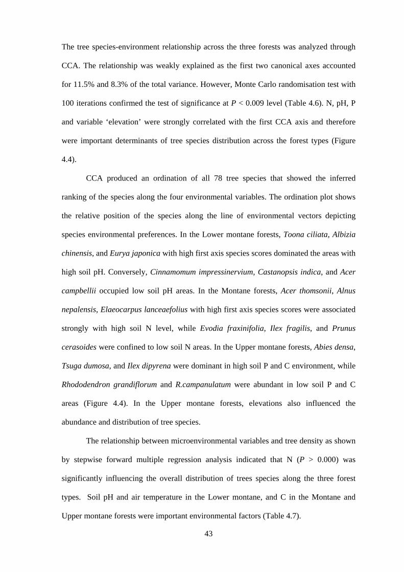
across the forest types (Figure 4.6).

Table 4.9. Variance explained in the Canonical Correspondence Analysis (CCA) for shrubs by the first two axes across the three forest types in KBR.

Axis 1 2 Total variance (inertia) in the tree species data

9.36


CCA produced an ordination of all 38 shrub species that showed the inferred

ranking of the species along the environmental variables. In the Lower montane forests,

Boehmeria macrophylla, Clerodendrum colebrokianum, and Dicranopteris linearis with

high first axis species scores dominated the areas with high soil pH. Conversely,

Boehmeria platyphylla, Debregeasia longifolia, and Edgeworthia gardneri occupied low

48

soil pH areas. In the Montane forests, Arundinaria maling, Berberis sikimensis,

Edgeworthia gardneri with high first axis species scores were strongly associated with

high soil C, P and K level, while Rosa sericea and Zanthoxylum oxyphyllum were

confined to low soil C, P and K areas. In the Upper montane forests, Juniperus recurva,

Rhododendron lepidotum, and Rhododendron setosum were dominant in high soil N

environment, while Arundinaria maling and Berberis sikkimensis were abundant in low

soil N areas (Figure 4.6).

The relationship between microenvironmental variables and shrub species density as

revealed by stepwise forward multiple regression analysis indicated that N (P > 0.000) is

significant in influencing the overall distribution of shrub species across the three forests.

In addition, light and soil C in the Lower montane, and soil C in the Montane and Upper

montane forests were important environmental variables (Table 4.10).

Figure 4.6. CCA ordination diagram using abundance data of 38 shrub species and microenvironmental variables from 60 plots across three forest types in KBR. The environmental variables are indicated by arrow and length of the arrow indicates the strength of the correlation. For clarity, species codes have been used which consist of the first three letter of the genus and the first letter of the species name; Acom-Aconogonum molle; Arum-Arundinaria maling; Bamn-Bambusa nutans; Bers-Berberis sikkimensis; Boem-Boehmeria macrophylla; Boep-Boehmeria platyphylla; Cleb-Clerodendrum colebrookianum; Dapb-Daphne bholua; Debl-Debregeasia longifolia; Desc-Desmodium confertum; Deuc-Deutzia compacta; Dicf-Dichroa febrifuga; Dicl-Dicranopteris linearis; Dobv-Dobinea vulgaris; Edgg-Edgeworthia gardneri; Elsf-Elsholtzia flava; Gird-Girardinia diversifolia; Gleg-Gleichenia glauca; Junr-Juniperus recurva; Lucg-Luculia gratissima; Maec-Maesa chisia; Maer-Maesa ramentacea; Melm-Melastoma malabathricum; Meln-Melastoma normale; Muet-Mussaenda treutleri; Nelr-Neillia rubriflora; Osbs-Osbeckia sikkimensis; Oxyp-Oxyspora paniculata; Pavi-Pavetta indica; Phoi-Photinia integrifolia; Rhoa-Rhododendron anthopogon; Rhol-Rhododendron lepidotum; Rhos-Rhododendron setosum; Ross-Rosa sericea; Rube-Rubus ellipticus; Rubm-Rubus mollucanus; Sama-Sambucus adnata; Thym-Thysaenolaena maxima; Zano-Zanthoxylum oxyphyllum.

49

Table 4.10. Results of forward stepwise multiple regression analysis of environmental variables with shrub density in three forest types in KBR.



Standard Error


Lower montane Light -0.356 -0.529 0.068 -5.205 0.000 -2.251 Carbon -2.503 -0.405 0.586 -4.271 0.001 Montane Carbon 6.380 0.597 2.019 3.160 0.005 -3.820 Upper montane Carbon 4.210 0.428 1.820 2.314 0.033 -5.485 Herbs

One hundred and thirty three species belonging to 97 genera and 49 families were

recorded from the three forest types. The number of species was highest in the Lower

montane forests (61) followed by the Montane (52) and Upper montane (39) forests

(Table 4.2). Herb species richness decreased with increasing elevation (R = -0.51; P <

0.05). The species diversity indices also decreased with increasing elevation (H = 3.93,

3.52, 3.23 and J = 0.95, 0.91 and 0.88 in the Lower montane, Montane and Upper

montane forests. The dominance index (D) also followed the same trend (D = 45.4, 28.1,

14.3). Fisher’s α diversity was greatest in the Lower montane forests, followed by Upper

montane and Montane forests (Table 4.3).

β-diversity was highest between the Lower montane and Upper montane (0.94),

followed by Montane and Upper montane (0.85) forests stands. Lower montane and

Montane forests had the lowest β-diversity value of (0.82).

Asteraceae and Poaceae were the dominant families in the Lower montane forests

(21.3% and 6.6%, respectively). Urticaceae, Lamiaceae and Polygonaceae each with

11.5%, 7.7% and 9.6% of the total species composition dominated the Montane forests.

Asteraceae, Polygonaceae each with 10.5% and 13.2% of the total species, dominated the

herb community in the Upper montane forests.

The three forest types differed significantly in herb species composition (Clark’s


50

Montane, Lower and Upper montane, and Montane and Upper montane forests was 99.1,

99.02 and 99.1%, respectively (Table 4.11). Anaphalis triplivnervis were found in all the

three forest types. Arundinella bengalensis, Athyrium rubicaule, Cyanotis vaga,

Dryopteris barbigera and Erigeron karvinskianus were confined to the Lower montane

and Montane forests. Arisaema griffithii, Fragaria nubicola, Galium elegans and

Hemiphragma heterophyllum were found only in the Montane and Upper montane forests

(Annexure 1).

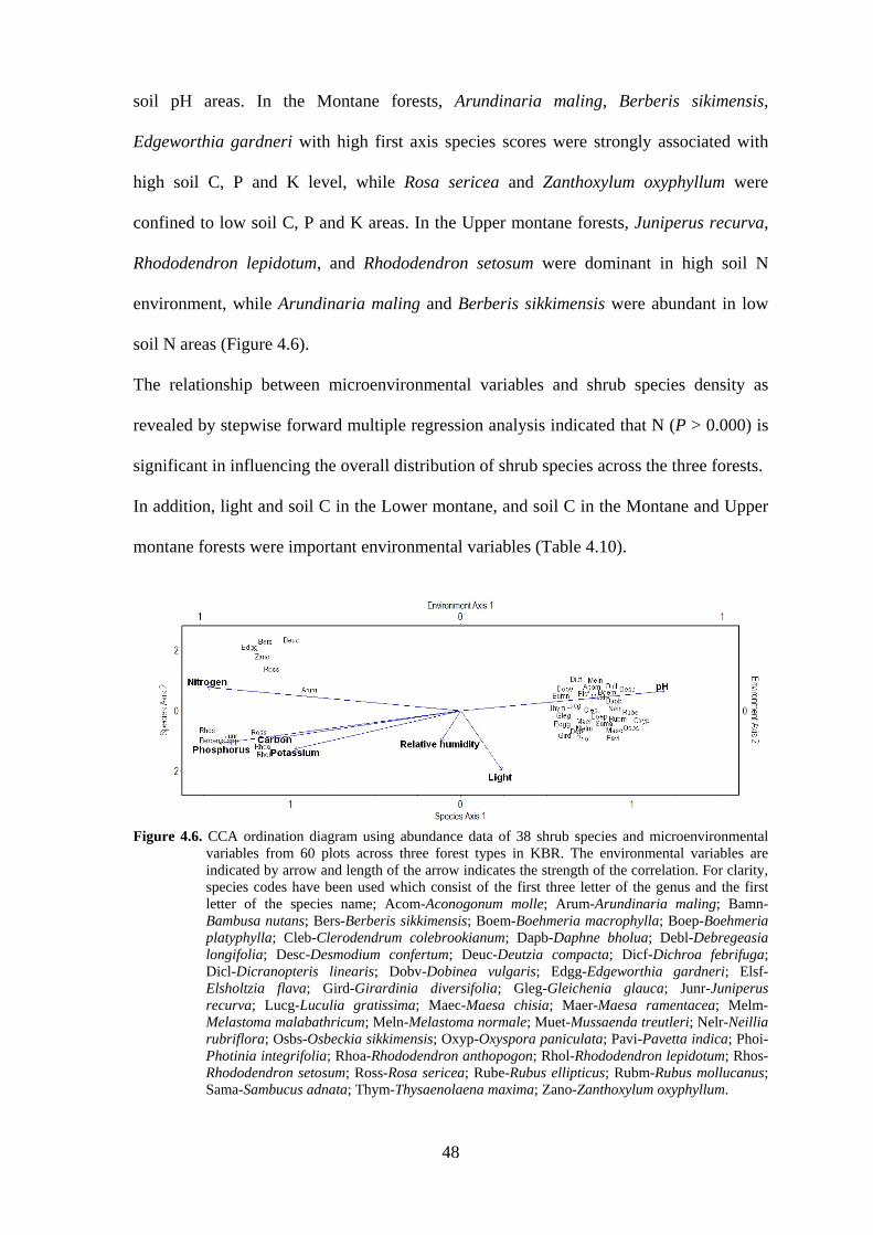
Table 4.11. Similarity test values of ANOSIM and SIMPER on the sampled sites for Lower montane, Montane and Upper montane forests areas. The ANOSIM ‘R value’ is the statistical value of similarity within each forest stands with a probability of 0.001.



Lower montane Montane 0.001 0.95 99.05 Lower montane Upper montane 0.001 0.98 99.02 Montane Upper montane 0.001 0.93 99.07 The density of herbaceous species did not differ significantly across the forests (F

= 0.90, P = 0.44). Highest density was in the Montane forests (711500 individual ha-1),

followed by the Upper montane and Lower montane forest stands (625000 individuals ha-

1 and 609500 individuals ha-1 respectively) (Table 4.2).

With an increase in elevation, the herb species-abundance curves exhibited higher

dominance (Figure 4.7). Four dominant and co-dominant herb species, Bidens pilosa, B.

biternata, Carex filicina, and Elsholtzia blanda together shared 27.5% of the total IVI

values in the Lower montane forests. Fragaria nubicola, Persicaria runcinata, Phlomis

bracteosa together shared 31.2% of the total IVI in the Montane forests while the

corresponding figure for Upper montane forests was much greater at 45.5%, which was

shared by Anaphalis triplinervis, Juncus spp., and Poa alpina (Annexure 1).

51

Figure 4.7. Dominance-diversity curve of herb species in Lower montane (LM), Montane (M) and Upper montane (UM) forests in KBR.

Microenvironmental factors related to herb abundance

Herb species-environment relationship across the forests was poorly explained as the first

two canonical axes accounted for 8.6 % and 6.1 % of the total variance. However, Monte

Carlo randomisation test with 100 iterations has also yielded a strong probability of 0.009

for both the axes indicating that the axes have explained a significant part of the

variability in the species abundance data (Table 4.12). N, C, pH, P and K were strongly

correlated with the first CCA axis and therefore were important determinants of herb

species distribution across the forest types (Figure 4.8).

Table 4.12. Variance explained in the Canonical Correspondence Analysis (CCA) for herbs by the first two axes across the forest types in KBR.

Axis 1 2 Total variance (inertia) in the tree species data

11.25


CCA produced an ordination of all 133 herb species that showed the inferred

ranking of the species along the above five environmental variables. The ordination plot

52

shows the relative position of the species along the line of environmental vectors

depicting species environmental preferences. In the Lower montane forests, Boehmeria

platyphylla, Cyanodon dactylon, Paspalum destichum, Pilea scripta, and Pogonatherum

paniceum with high first axis species scores dominated the areas with high soil pH.

Conversely, Arundinella bengalensis, Cuphea balsamona, Cyanotis vaga, and

Desmodium multiflorum occupied low soil pH areas. In the Montane forests, Impatiens

urticifolia, Sanicula elata, Oxalis acetosella, Viola biflora with high first axis species

scores were associated strongly with high soil N level, while Ainsliaea aptera and

Arundinella bengalensis were confined to low soil N areas. In the Upper montane forests,

Arisaema jacquemontii, Poa himalayana, and Potentilla eriocarpa were dominant in high

soil P, K and C environment, while Juncus spp., Megacodon stylophorus, and Bistorta

affinis were abundant in low soil P, K and C areas (Figure 4.8).

The relationship between microenvironmental variables and herb species density

as shown by stepwise forward multiple regression analysis indicated that P (P < 0.031) is

significant in influencing the overall distribution of herb species along the three forests.

Forest wise, pH and elevations in the Lower montane, and N, P in the Montane and P

alone in the Upper montane forests were important (Table 4.13).

53

Figure 4.8. CCA ordination diagram using abundance data of 133 herb species and microenvironmental

variables from 60 plots across three forest types in KBR. The environmental variables are indicated by arrow and length of the arrow indicates the strength of the correlation. For clarity, species codes have been used which consist of the first three letter of the genus and the first letter of the species name; Acha-Achyranthes aspera; Acos-Aconitum spicatum; Agrp-Agrimonia pilosa; Aina-Ainsliaea aptera; Alep-Aletris pauciflora; Anab-Anaphalis busua; Anam-Anaphalis margaritacea; Anat-Anaphalis triplinervis; Anas-Anisadenia saxatilis; Anii-Anisomeles indica; Antg-Anthogonium gracile; Aric-Arisaema concinnum; Arig-Arisaema griffithii; Arij-Arisaema jacquemontii; Artn-Artemisia nilagirica; Artv-Artemisia vulgaris; Arub-Arundinella bengalensis; Astr-Astilbe rivularis; Athr-Athyrium rubricaule; Begj-Begonia josephii; Begr-Begonia rubrella; Bidb-Bidens biternata; Bidp-Bidens pilosa; Bisa-Bistorta affinis; Bupl-Bupleureum longicaule; Calp-Caltha palustris; Camp-Campanula pallida; Cama-Campylandra aurantiaca; Carf-Carex filicina; Caug-Cautleya gracilis; Chln-Chlorophytum nepalense; Chrc-Chrysosplenium carnosum; Cirv-Cirsium verutum; Cliu-Clintonia udensis; Conc-Coniogramme cautata; Craf-Craniotome furcata; Cupb-Cuphea balsamona; Cynv-Cyanotis vaga; Cyac-Cyathula capitata; Cynd-Cynodon dactylon; Cypn-Cyperus niveus; Cypr-Cyperus rotundus; Desm-Desmodium multiflorum; Dici-Dicrocephala integrifolia; Dryb-Dryopteris barbigera; Dryopteris spp.; Elao-Elatostemma obtusum; Elap-Elatostemma platyphylla; Elas-Elatostemma sessile; Elsb-Elsholtzia blanda; Elsf-Elsholtzia fruticosa; Equd-Equisetum diffusum; Erib-Erogeron bellidioides; Erik-Erigeron karvinskianus; Eupc-Eupatorium cannabinum; Eups-Euphorbia sikkimensis; Fran-Fragaria nubicola; Fric-Fritillaria cirrhosa; Gala-Galium asperifolium; Gale-Galium elegans; Galm-Galium mullago; Gern-Geranium nepalense; Gnal-Gnaphalium luteo-album; Gonh-Gonostegia hirta; Gync-Gynura cusimba; Hacu-Hackelia uncinata; Heds-Hedychium spicatum; Heds-Hedyotis scandans; Hemh-Hemiphragma heterophyllum; Herl-Herminium lanceum; Hydn-Hydrocotyle nepalensis; Hype-Hypericum elodeoides; Hypt-Hypoestes triflora; Hypa-Hypoxis aurea; Impatiens spp.; Juncus spp.; Knos-Knoxia sumatrensis; Lecp-Lecanthus peduncularis; Leui-Leucostegia immerse; Miap-Maianthemum purpureum; Mecv-Meconopsis villosa; Megs-Megacodon stylophorus; Mimn-Mimulus nepalensis; Noth-Notochaete hamosa; Oplc-Oplismenus compositus; Osbs-Osbeckia stellata; Oxaa-Oxalis acetosella; Oxac-Oxalis corniculata; Panp-Panax pseudoginseng; Parm-Pardavallodes multidentum; Parp-Paris polyphylla; Pasd-Paspalum destichum; Perc-Persicaria capitata; Perc-Persicaria chinense; Perp-Persicaria polystachya; Perr-Persicaria runcinata; Phlb-Phlomis bracteosa; Pils-Pilea scripta; Pils-Pilea symmeria; Pilu-Pilea umbrosa; Plae-Plantago erosa; Poaa-Poa annua; Poah-Poa himalayana; Pogp-Pogonatherum paniceum; Polh-Polygonum hydropiper; Polp-Polygonum plebium; Polp-Polystichum prescotianum; Pota-Potentilla arbuscula; Pote-Potentilla eriocarpa; Pric-Primula capitata; Pric-Primula caveana; Pteris spp.; Rand-Ranunculus diffusus; Ranp-Ranunculus pulchellus; Rhea-Rheum acuminatum; Rubm-Rubus mollucanus; Rumn-Rumex nepalensis; Sane-Sanicula elata; Scod-Scoparia dulcis; Selt-Selenium tenuifolium; Send-Senecio diversifolius; Senw-Senecio wallichii; Spip-Spilanthes paniculatus; Stes-Stellaria sikkimensis; Swec-Swertia chirayita; Urtd-Urtica dioica; Valh-Valeriana hardwickii; Viob-Viola biflora; Viop-Viola pilosa.

54

Table 4.13. Results of forward stepwise multiple regression analysis of environmental variables with herb density in the three forest types in KBR.



Standard Error


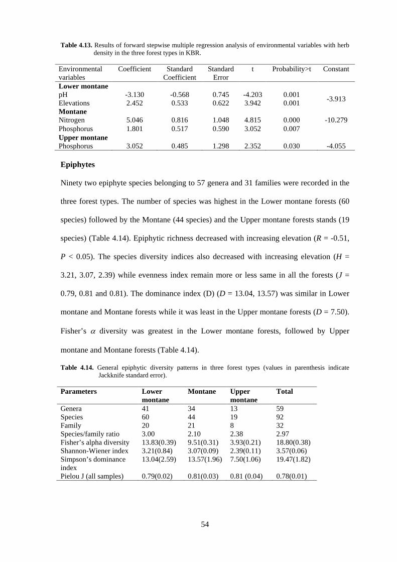
Lower montane pH -3.130 -0.568 0.745 -4.203 0.001 -3.913 Elevations 2.452 0.533 0.622 3.942 0.001 Montane Nitrogen 5.046 0.816 1.048 4.815 0.000 -10.279 Phosphorus 1.801 0.517 0.590 3.052 0.007 Upper montane Phosphorus 3.052 0.485 1.298 2.352 0.030 -4.055 Epiphytes

Ninety two epiphyte species belonging to 57 genera and 31 families were recorded in the

three forest types. The number of species was highest in the Lower montane forests (60

species) followed by the Montane (44 species) and the Upper montane forests stands (19

species) (Table 4.14). Epiphytic richness decreased with increasing elevation (R = -0.51,

P < 0.05). The species diversity indices also decreased with increasing elevation (H =

3.21, 3.07, 2.39) while evenness index remain more or less same in all the forests (J =

0.79, 0.81 and 0.81). The dominance index (D) (D = 13.04, 13.57) was similar in Lower

montane and Montane forests while it was least in the Upper montane forests (D = 7.50).

Fisher’s α diversity was greatest in the Lower montane forests, followed by Upper

montane and Montane forests (Table 4.14).

Table 4.14. General epiphytic diversity patterns in three forest types (values in parenthesis indicate Jackknife standard error).

Parameters Lower

montane Montane Upper

montane Total

Genera 41 34 13 59 Species 60 44 19 92 Family 20 21 8 32 Species/family ratio 3.00 2.10 2.38 2.97 Fisher’s alpha diversity 13.83(0.39) 9.51(0.31) 3.93(0.21) 18.80(0.38) Shannon-Wiener index 3.21(0.84) 3.07(0.09) 2.39(0.11) 3.57(0.06) Simpson’s dominance index

13.04(2.59) 13.57(1.96) 7.50(1.06) 19.47(1.82)

Pielou J (all samples) 0.79(0.02) 0.81(0.03) 0.81 (0.04) 0.78(0.01)

55

The species: family ratio in the Lower montane (3.00) was also higher compared to

Montane (2.10) and Upper montane (2.38) epiphyte species. The Pteridophytic family,

Polypodiaceae (21 species, 21.9%) was the dominant family followed by Orchidaceae (19

species, 19.8%) across the forest types. It had 67% of total species in the Lower montane,

50.5% in the Montane and 20.8% in the Upper montane forests. Pteridophytic families

were dominant in the Upper montane (66.7%) and the Montane (58.3%) forest stands.

β-diversity was highest between the Lower and the Upper montane (0.90), followed by

Lower montane and Montane (0.65) forests. Upper montane and Montane forests had the

least β-diversity value of (0.62).

The three forest types differed significantly in epiphyte species composition

(Clark’s R statistic = 0.47, P < 0.001). Species dissimilarity between Lower montane and

Montane, Lower and Upper montane, and Montane and Upper montane forests was

95.05, 97.05 and 89.68%, respectively (Table 4.15).

In general, pteridophytic species were dominant epiphytic community in all the

forest stands. Dominant species from the Lower montane forests stand were Hoya

linearis, Lepisorus nudus, Mecodium spp., Peperomia tetraphylla and Vittaria elongata.

Lepisorus nudus, Pleione humilis, Vaccinium retusum and Vittaria elongata were

dominant in the Montane forests. While in the Upper montane forests, the dominant

species were Onychium spp., Cystopteris sudetica, Pleione humilis, Phymatopteris

malacodon and Vaccinium nummularia (Annexure 2).

The prevalence of epiphytes like Hoya linearis (14.1%), Pleione humilis (9.3%)

and Vittaria elongataa (8.1%) were the main contributors to the dissimilarity between the

Lower montane and the Montane forests. A high abundance of Hoya linearis (15.6%),

Lepisorus nudus (7.9%) and Onychium spp., (1.9%) was the cause of dissimilarity

between the Lower montane and the Upper montane forests. Between the Montane and

56

Upper montane forests, the main cause of dissimilarity was the high abundance of

Pleione humilis (12.5%), Onychium spp., (8.9%) and Vittaria elongata (8.8%).

Table 4.15. Similarity test values of ANOSIM and SIMPER in the sampled sites for Lower montane, Montane and Upper montane forests. The ANOSIM ‘R value’ is the statistical value of similarity within each forest stands with a probability of 0.001.

All stands together R value P value 0.47 0.001 Stand wise test (No. of quadrats) 1st group 2nd group P value ANOSIM(R

value) SIMPER(average dissimilarity)


The density of epiphytes decreased significantly across the forest types (F = 8.53,

P < 0.001). It was highest in the Lower montane forests (5200 individuals 20 tree-1),

followed by the Montane and the Upper montane forests (4830 and 2390 individuals 20

tree-1 respectively) (Annexure 2).

With an increase in elevation, the epiphyte species-abundance curves exhibited

higher dominance (Figure 4.9). Dominance-diversity curves for epiphyte species showed

that most IVI values in the Upper montane forests were concentrated in two species viz.

Cystopteris sudetica and Onychium spp. In the Lower montane and Montane forests IVI

was distributed more equitably among all the species than the Upper montane forests

(Figure 4.9). The three dominant and codominant epiphyte species in the Lower montane

forests viz. Hoya linearis, Lepisorus nudus and Vittaria elongata together shared 57.9 %

of the total IVI values. In the Montane forests the three dominants species viz. V.

elongata, L. nudus and Pleione humilis together shared 59 % of the total IVI. In the

Upper montane forests, Cystopteris sudetica, Onychium spp., and P. humilis shared

90.6% of the total IVI. The Pteridophytic family Polypodiaceae (21 species, 21.9 %) was

the dominant family followed by Orchidaceae (19 species, 19.8 %) across the forest

types. Pteridophytic families were also dominant in the Upper montane (66.7 %) and

Montane (58.3 %) forests (Annexure 2).

57

nMDS - Axis 1 vs Axis 2 - 2D Model, Rotated, Bray-Curtis

2D Stress = 0.148677

Axis 143210-1

Axi

s 2

1

0

-1

Figure 4.9. Dominance-diversity curves for epiphyte species in Lower montane (LM), Montane (M) and Upper montane (UM) forests in KBR.

Non-Metric Multi Dimensional Scaling

The nMDS ordination resulted in a three dimensional solution with a moderately low

stress (2D stress = 0.148) and a small amount of overlap between cluster group scores.

The nMDS of three forest types using the abundance data of the species in this case

showed that the Montane epiphytic species are more common to both the Lower and the

Upper montane epiphytic species (Figure 4.10).

Figure 4.10. Non metric multi dimensional scaling (nMDS) plot for epiphytic species using Bray-Curtis index of similarity of their abundance data from Lower montane (LM), Montane (M) and Upper montane (UM) forests in KBR. The classification showing the distribution pattern of the species in the three forest types is distinct (T-indicates tree host).

All the species were classified by lifeform (growth habit) and by taxonomic group

(Figure 4.11). Most epiphytes belonged to Caespitose followed by pendent life form.

58

Figure 4.11. Distribution of epiphytes in different life forms in KBR.

According to habit or taxonomic classification, epiphytes consisted of three

different groups. The pteridophytic community was the highest with 40.2%, followed by

herbaceous epiphytes (33.7%), shrubs and climbers (19.6%) and under tree (5.4%). True

epiphytes need hosts where they start and saturate their life cycle and do not destroy or

overcast the host. Whereas false epiphytes grow on selective hosts and later on become

independent by sending roots to the ground (Table 4.16). True epiphytes were mostly

herbaceous epiphytes such as Peperomia tetraphylla, P.heyneana, Pilea racemosa, P.

approximata, P. ternifolia, ferns and Begonia gemmipara.

The shrubby epiphytes include Aeschynanthus spp., Hoya spp., Hymenopogon

parasiticus, Hymenodictyon excelsum, H. flaccidum, Piper mullesua, Lysionotus

atropurpureus, Vaccninium vacciniaceum, Agapetes serpens, A. sikkimensis, and R.

vaccinioides. The climbing epiphytes are Hoya fusca, Piper longum, Schefflera

benghalensis and some Ficus species.The epiphytic trees are mostly false epiphytes. The

examples are Ficus spp., Hymenopogon parasiticus, Macropanax undulatus, M.

dispermus, Pentapanax fragrans, P. racemosus, Rhododendron dalhousiae, Vaccinium

spp., and Wightia speciosissima.

59

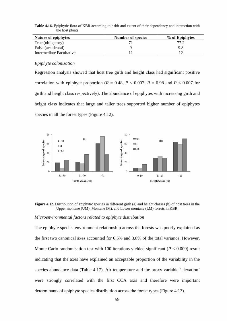
Table 4.16. Epiphytic flora of KBR according to habit and extent of their dependency and interaction with the host plants.

Nature of epiphytes Number of species % of Epiphytes True (obligatory) 71 77.2 False (accidental) 9 9.8 Intermediate Facultative 11 12 Epiphyte colonization

Regression analysis showed that host tree girth and height class had significant positive

correlation with epiphyte proportion (R = 0.48, P < 0.007; R = 0.98 and P < 0.007 for

girth and height class respectively). The abundance of epiphytes with increasing girth and

height class indicates that large and taller trees supported higher number of epiphytes

species in all the forest types (Figure 4.12).

Figure 4.12. Distribution of epiphytic species in different girth (a) and height classes (b) of host trees in the Upper montane (UM), Montane (M), and Lower montane (LM) forests in KBR.

Microenvironmental factors related to epiphyte distribution

The epiphyte species-environment relationship across the forests was poorly explained as

the first two canonical axes accounted for 6.5% and 3.8% of the total variance. However,

Monte Carlo randomisation test with 100 iterations yielded significant (P < 0.009) result

indicating that the axes have explained an acceptable proportion of the variability in the

species abundance data (Table 4.17). Air temperature and the proxy variable ‘elevation’

were strongly correlated with the first CCA axis and therefore were important

determinants of epiphyte species distribution across the forest types (Figure 4.13).

60

CCA produced an ordination of all 92 epiphyte species that showed the inferred

ranking of the species along the four environmental variables. The ordination plot shows

the relative position of the species along the line of environmental vectors depicting

species environmental preferences. In the Lower montane forests, Ficus spp., Hoya fusca,

Remusatia hookeriana, and Vandopsis undulata with high first axis species scores were

correlated with elevation. Conversely, Davallia bullata, Medinilla himalayana, and

Pyrrosia lehmanii were correlated with RH in second axis. In the Montane forests,

Bulbophyllum reptans, Lepisorus kashyapii, Lepisorus nudus, and Pilea lineolatum, with

high second axis species scores were associated strongly with high light level and RH,

while Codonopsis purpurea, Didymocarpus aromaticus, Rhododendron pumilum and

Utricularia multicaulis were confined to low light and RH areas. In the Upper montane

forests, Cystopteris sudetica, Phymatopteris malacodon, and Pholidotia spp., were

dominant in high air temperature environment, while Arthomeris wallichii, Lepisorus

scolopendrinus and Vaccinium nummularia were abundant in low air temperature (Figure

4.13).

Table 4.17. Variance explained in the Canonical Correspondence Analysis (CCA) for epiphyte by the first two axes across the forest types in KBR.

Axis 1 2 Total variance (inertia) in the epiphyte species data

10.22


61

Species Axis 110-1

Environment Axis 110-1

Spe

cies

Axi

s 2

2

0

-2

Environm

ent Axis 2

0

Figure 4.13. CCA ordination diagram using abundance data of 92 epiphyte species and microenvironmental variables from 60 plots across three forest types in KBR. The environmental variables are indicated by arrow and length of the arrow indicates the strength of the correlation. For clarity, species codes have been used which consist of the first three letter of the genus and the first letter of the species name; Aesb-Aeschynanthus bracteatus; Aesh-Aeschynanthus hookeri; Aess-Aeschynanthus sikkimensis; Agah-Agapetes hookeri; Agai-Agapetes incurvata; Agas-Agapetes serpens; Agrb-Agrostophyllum brevipes Agrc-Agrostophyllum callosum; Arth-Arthomeris himalayensis; Artl-Arthomeris lehmanii; Artw-Arthomeris wallichiana; Aspe-Asplenium ensiforme; Bels-Belvisia spicata; Bulc-Bulbophyllum cauliflorum; Bulr-Bulbophyllum reptans; Caug-Cautleya gracilis; Chef-Cheilanthes formosana; Codp-Codonopsis purpurea; Coec-Coelogynae corymbosa; Coeo-Coelogynae ochracea; Cyss-Cystopteris sudetica; Davb-Davallia bullata; Dena-Dendrobium amoenum; Denl-Dendrobium longicornu; Denn-Dendrobium nobile; Dida-Didymocarpus aromaticus; Dido-Didymocarpus oblongus; Dryp-Drynaria propinqua; Eric-Eria coronaria; Eris-Eria spicata; Ficus spp.; Gloh-Globa hookeri; Gonp-Gonatanthus pumilus; Hoyf-Hoya fusca; Hoyl-Hoya lanceolata; Hoyli-Hoya linearis; Hymp-Hymenopogon parasiticus; Lepk-Lepisorus kashyapii; Lepn-Lepisorus nudus; Lepsc-Lepisorus scolopendrinus; Leps-Lepisorus sesquepedalis; Leui-Leucostegia immersa; Lino-Lindsaea odorata; Lipp-Lipparis perpusilla; Loxi-Loxogramme involuta; Lycopodium spp.; Lyss-Lysionotus serratus; Macu-Macropanax undulatum; Mecodium spp.; Medh-Medinilla himalayana; Micm-Microsorium membranaceum; Micp-Microsorium puctatum; Nepc-Nephrolepis cordifolia; Olew-Oleandra wallichii; Onychium spp.; Oto-Otochilus alba; Penl-Pentapanax leschenaultii; Penr-Pentapanax racemosus; Peph-Peperomia heyneana; Pept-Peperomia tetraphylla; Phat-Phalaenopsis tainitis; Phlp-Phlegmariurus phlegmaria; Phoi-Pholidota imbricata; Pholidota spp.; Phye-Phymatopteris ebinipes; Phym-Phymatopteris malacodon; Phyo-Phymatopteris oxyloba; Pill-Pilea lineolatum; Pleh-Pleione hookeriana; Pleh-Pleione humilis; Pola-Polypodiastrum argutum; Pola-Polypodioides amoena; Poll-Polypodioides lachnopus; Pyrf-Pyrrosia flocculosa; Pyrl-Pyrrosia lanceolata; Pyrs-Pyrrosia stigmosa; Remh-Remusatia hookeriana; Rhop-Rhododendrom pendulum; Rhod-Rhododendron dalhousiae; Ross-Roscoea spicata; Selaginella spp.; Smio-Smilacina oleracea; Utrm-Utricularia multicaulis; Vacn-Vaccinium nummularia; Vacr-Vaccinium retusum; Vacv-Vaccinium vacciniaceum; Vanu-Vandopsis undulata; Vite-Vittaria elongata; Vitf-Vittaria flexuosa; Vith-Vittaria himalayensis; Vits-Vittaria sikkimensis; Wigs-Wightia speciosissima.

The relationship between microenvironmental variables and epiphyte density as

shown by stepwise forward multiple regression analysis indicated that elevation (P <

0.010) is significant in influencing the overall distribution of epiphyte species along the

forest types. In addition, light in the Lower montane, elevation in the Montane and RH in

the Upper montane forests were important environmental factors (Table 4.18).

62

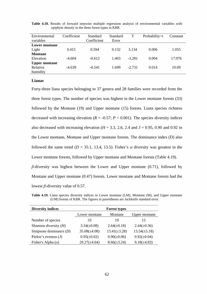
Table 4.18. Results of forward stepwise multiple regression analysis of environmental variables with epiphyte density in the three forest types in KBR.



Standard Error

T Probability>t Constant

Lower montane Light 0.415 0.594 0.132 3.134 0.006 1.055 Montane Elevation -4.604 -0.612 1.403 -3.281 0.004 17.076 Upper montane Relative humidity

-4.639 -0.541 1.699 -2.731 0.014 10.09

Lianas

Forty-three liana species belonging to 37 genera and 28 families were recorded from the

three forest types. The number of species was highest in the Lower montane forests (33)

followed by the Montane (19) and Upper montane (15) forests. Liana species richness

decreased with increasing elevation (R = -0.57; P < 0.001). The species diversity indices

also decreased with increasing elevation (H = 3.3, 2.6, 2.4 and J = 0.95, 0.90 and 0.92 in

the Lower montane, Montane and Upper montane forests. The dominance index (D) also

followed the same trend (D = 35.1, 13.4, 13.5). Fisher’s α diversity was greatest in the

Lower montane forests, followed by Upper montane and Montane forests (Table 4.19).

β-diversity was highest between the Lower and Upper montane (0.71), followed by

Montane and Upper montane (0.47) forests. Lower montane and Montane forests had the

lowest β-diversity value of 0.57.

Table 4.19. Liana species diversity indices in Lower montane (LM), Montane (M), and Upper montane (UM) forests of KBR. The figures in parentheses are Jackknife standard error.

Diversity indices Forest types Lower montane Montane Upper montane Number of species 33 19 15 Shannon diversity (H) 3.34(±0.08) 2.64(±0.18) 2.44(±0.36) Simpsons dominance (D) 35.08(±4.08) 13.41(±3.28) 13.54(±5.18) Pielou’s eveness (J) 0.95(±0.02) 0.90(±0.06) 0.92(±0.04) Fisher's Alpha (α) 20.27(±4.64) 8.66(±3.24) 9.18(±4.83)

63

Vitaceae was the dominant family in the Lower montane (11.7%) and Montane (10%)

forests. Caprifoliaceae, Schisandraceae and Ranunculaceae, each with 13.3% of the total

species, dominated the liana community in Upper montane forests.

The three forest types differed significantly in liana species composition (Clark’s


Montane, Lower and Upper montane, and Montane and Upper montane forests was 61,

99.2 and 99%, respectively. Clematis buchananiana, Embelia floribunda, Holboellia

latifolia, Hydrangea anomala, Lonicera glabrata, Rubus paniculatus and Tetrastigma

serrulatum were found in all the three forest types. Dicentra scandens, Gnetum

montanum, Hedera nepalensis, Micrechites elliptica, Parthenocissus himalayana and

Piper mullesua, were confined to lower Montane and Montane forests. Actinidia callosa,

Schisandra grandiflora and Zanthoxylum oxyphyllum were found only in Montane and

Upper montane forests (Table 4.20).

The density of lianas decreased from 83 stems ha-1 in the lower montane forests to

73 stems ha-1 in the montane and 38 stems ha-1 in the upper montane forests (F = 70.18, P

< 0.001). The basal area of lianas also followed a similar trend, i.e. 3.54, 2.25 and 0.13 m2

ha-1 in the Lower montane, Montane and Upper montane forests, respectively.

64

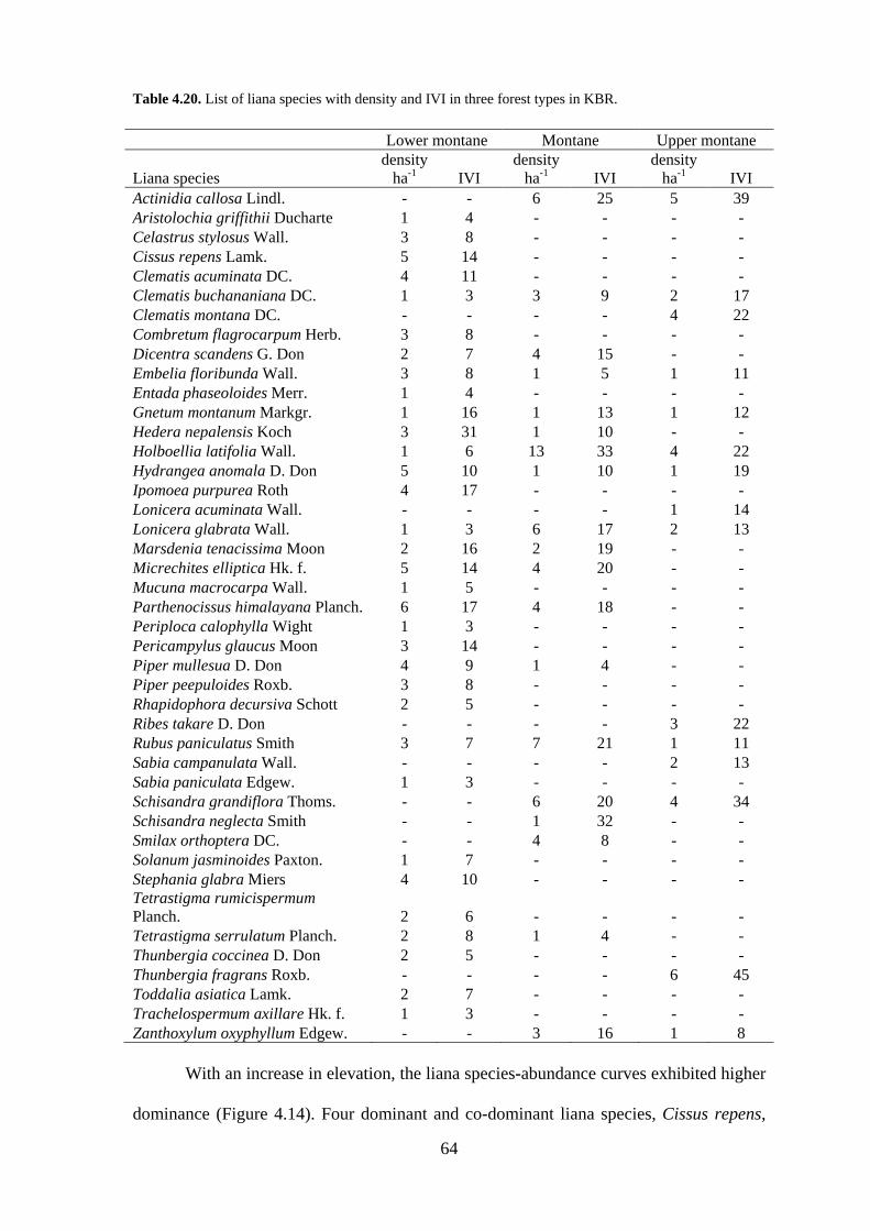
Table 4.20. List of liana species with density and IVI in three forest types in KBR.

With an increase in elevation, the liana species-abundance curves exhibited higher

dominance (Figure 4.14). Four dominant and co-dominant liana species, Cissus repens,

Lower montane Montane Upper montane

Liana species density

ha-1 IVI density

ha-1 IVI density

ha-1 IVI Actinidia callosa Lindl. - - 6 25 5 39 Aristolochia griffithii Ducharte 1 4 - - - - Celastrus stylosus Wall. 3 8 - - - - Cissus repens Lamk. 5 14 - - - - Clematis acuminata DC. 4 11 - - - - Clematis buchananiana DC. 1 3 3 9 2 17 Clematis montana DC. - - - - 4 22 Combretum flagrocarpum Herb. 3 8 - - - - Dicentra scandens G. Don 2 7 4 15 - - Embelia floribunda Wall. 3 8 1 5 1 11 Entada phaseoloides Merr. 1 4 - - - - Gnetum montanum Markgr. 1 16 1 13 1 12 Hedera nepalensis Koch 3 31 1 10 - - Holboellia latifolia Wall. 1 6 13 33 4 22 Hydrangea anomala D. Don 5 10 1 10 1 19 Ipomoea purpurea Roth 4 17 - - - - Lonicera acuminata Wall. - - - - 1 14 Lonicera glabrata Wall. 1 3 6 17 2 13 Marsdenia tenacissima Moon 2 16 2 19 - - Micrechites elliptica Hk. f. 5 14 4 20 - - Mucuna macrocarpa Wall. 1 5 - - - - Parthenocissus himalayana Planch. 6 17 4 18 - - Periploca calophylla Wight 1 3 - - - - Pericampylus glaucus Moon 3 14 - - - - Piper mullesua D. Don 4 9 1 4 - - Piper peepuloides Roxb. 3 8 - - - - Rhapidophora decursiva Schott 2 5 - - - - Ribes takare D. Don - - - - 3 22 Rubus paniculatus Smith 3 7 7 21 1 11 Sabia campanulata Wall. - - - - 2 13 Sabia paniculata Edgew. 1 3 - - - - Schisandra grandiflora Thoms. - - 6 20 4 34 Schisandra neglecta Smith - - 1 32 - - Smilax orthoptera DC. - - 4 8 - - Solanum jasminoides Paxton. 1 7 - - - - Stephania glabra Miers 4 10 - - - - Tetrastigma rumicispermum Planch. 2 6 - - - - Tetrastigma serrulatum Planch. 2 8 1 4 - - Thunbergia coccinea D. Don 2 5 - - - - Thunbergia fragrans Roxb. - - - - 6 45 Toddalia asiatica Lamk. 2 7 - - - - Trachelospermum axillare Hk. f. 1 3 - - - - Zanthoxylum oxyphyllum Edgew. - - 3 16 1 8

65

Clematis acuminata, Hydrangea anomala and Parthenocissus himalayana together

shared 23% of the total IVI values in the Lower montane forests while the corresponding

figure for Montane forests was much greater at 42% which was shared by Actinidia

callosa, Holboellia latifolia, Rubus paniculatus, and Schisandra grandiflora. It further

increased to 57% in Upper montane forests which were shared by A. callosa, Clematis

Montana, H. latifolia, Schisandra neglecta, and S. grandiflora (Table 4.20).

Figure 4.14. Liana dominance diversity curves in Lower montane (LM), Montane (M) and Upper montane (UM) forests in KBR.

Microenvironmental factors related to liana density

The species-environment relationship across the forests was poorly explained as the first

two canonical axes accounted for 7.6 % and 6.8 % of the total variance. Nevertheless,

Monte Carlo randomisation test with 100 iterations has yielded a probability of 0.009 for

both the axes indicating that the axes have explained a significant part of the variability in

the species abundance data (Table 4.21).

Light, soil pH, N, P and variable ‘elevation’ were strongly correlated with the first

CCA axis and therefore were important determinants of liana species distribution across

the forest types (Figure 4.15). CCA produced an ordination of all 43 species that showed

the inferred ranking of the species along the environmental variables. The ordination plot

shows the relative position of the species along the line of environmental vectors

depicting species environmental preferences. In the Lower montane forests, Combretum

66

flagrocarpum, Hedera nepalensis, and Holboellia latifolia with high first axis species

scores dominated the areas with high soil pH. Conversely, C. buchananiana, Entada

phaseoloides, and Sabia paniculata occupied low soil pH areas. In the Montane forests,

A. callosa, C. buchananiana, L. glabrata, S. grandiflora and Z. oxyphyllum with high first

axis species scores were associated strongly with high soil N level, while H. nepalensis,

Hydrangea anomala, and Marsdenia tenacissima were confined to low soil N areas. In

the Upper montane forests, Actinidia callosa, H. latifolia, Sabia campanulata and

Thunbergia fragrans were dominant in high soil P environment, while H. anomala, L.

acuminata and Z. oxyphyllum were abundant in low soil P areas (Figure 4.15).

The relationship between microenvironmental variables and adult liana density as

shown by stepwise forward multiple regression analysis, indicated that light in the Lower

montane, soil P concentration in the Montane, and both light and soil P in the Upper

montane forests were important determinants of liana abundance (Table 4.22).

Table 4.21. Variance explained in the Canonical Correspondence Analysis (CCA) by the first two axes across the forest types in KBR.

Axis 1 2 Total variance in species data 13.07 Sum of canonical eigen values 3.85 Sum of non canonical eigen values 9.21 Canonical eigen value 0.99 0.89 % variance explained 7.57 6.83 Cumulative % variance 7.57 14.41 Probability (Monte Carlo test) 0.009 0.009 Non-canonical eigen value 0.80 0.77 % variance explained 6.15 5.89 Cumulative % variance 6.15 12.05 Table 4.22. Results of forward stepwise multiple regression analysis of environmental variables with liana

density in the three forest types in KBR. Environmental variables


Standard Error


Lower montane Light 0.841 0.955 0.092 9.125 0.000 -0.030 Montane Soil phosphorus 0.880 0.836 0.204 4.312 0.003 -0.235 Upper montane Light 0.676 0.548 0.214 3.160 0.016 -0.762 Soil phosphorus 0.576 0.554 0.180 3.194 0.015

67

Figure 4.15. CCA ordination diagram using abundance data of 43 liana species and microenvironmental variables from 30 plots across three forest types in KBR. The environmental variables are indicated by arrow and length of the arrow indicates the strength of the correlation. For clarity, species codes have been used which consist of the first three letter of the genus and the first letter of the species name; Actc- Actinidia callosa; Arig- Aristolochia griffithii; Cels- Celastrus stylosus; Cisr- Cissus repens; Clea- Clematis acuminata; Cleb- Clematis buchananiana; Clem- Clematis montana; Comf- Combretum flagrocarpum; Dics- Dicentra scandens; Embf- Embelia floribunda; Entp- Entada phaseoloides; Gnem- Gnetum montanum; Hedn- Hedera nepalensis; Holl- Holboellia latifolia; Hyda- Hydrangea anomala; Ipop- Ipomoea purpurea; Lona- Lonicera acuminata; Long- L. glabrata; Mart- Marsdenia tenacissima; Mice- Micrechites elliptica; Mucm- Mucuna macrocarpa; Parh- Parthenocissus himalayana; Perc- Periploca calophylla; Perg- Pericampylus glaucus; Pipm- Piper mullesua; Pipp- P. peepuloides; Rhad- Rhapidophora decursiva; Ribt- Ribes takare; Rubp- Rubus paniculatus; Sabc- Sabia campanulata; Sabp- S. paniculata; Schg- Schisandra grandiflora; Schn- S. neglecta; Smio- Smilax orthoptera; Solj- Solanum jasminoides; Steg- Stephania glabra; Tetr- Tetrastigma rumicispermum; Tets- T. serrulatum; Thuc- Thunbergia coccinea; Thuf- T. fragrans; Toda- Toddalia asiatica; Traa- Trachelospermum axillare; Zano- Zanthoxylum oxyphyllum.

Discussion

The species diversity and richness pattern of different vegetation components in three

forests were largely influenced by elevation. Lower montane forests had higher diversity

in terms of family, genera and species in comparison to Montane and Upper montane

forests. The three forest types were endowed with a number of threatened plant species

(Table 4.23 and Plate 4.1). Considerable differences in floristic composition among the

plant communities in different forest types indicate the important role of prevailing

environmental conditions in determining species composition. A decreasing trend in

species richness with elevation has been reported by several earlier workers (Yoda 1967;

Odland & Birks 1999; Grytnes et al. 2002). It is obvious that the forests in KBR are

68

strongly correlated with elevation; which is found to be in accordance with the general

elevation pattern of ecosystem formation (Richerson et al. 1980). Elevation gradient

produce diverse climates, along with resultant soil differentiation, promoting the

diversification of plant species (Brown 2001; Lomolino 2001).

Table 4.23. List of Rare and Threatened plants in three forests.

Plant species Forest types IUCN category Acer hookeri Miq. Lower montane Rare Aconitum ferox Wall. Upper montane Endangered Arisaema griffithii Griffith. Montane Vulnerable Aristolochia griffithii Ducharte Lower montane/Montane Vulnerable Campylandra aurantiaca Baker Lower montane/Montane Endangered Cardiocrinum giganteum (Wall.) Makino Lower montane Rare Ceropegia hookeri Clarke Montane Critically rare Nardostachys grandiflora DC. Upper montane Critically rare Panax pseudo-ginseng Wall. Upper montane Lower risk Rheum nobile Hook. f. Upper montane Endangered Rhododendron anthopogon D. Don Upper montane Vulnerable Rhododendron maddenii Hook.f. Montane Rare

Whittaker (1972, 1977), MacArthur (1965), Wilson & Shmida (1984) and Brokaw

& Scheiner (1989) have discussed the importance of α- and β-diversity in explaining the

species richness of a plant community. Higher α- diversity of trees, herbs and lianas in

the Lower montane forests, indicates the existence of a wide range of vegetation

formation such as lowland forest, transitional forest, and riverine forests besides the

upland mountain forests. These diverse formations have contributed to high species

richness in this forest. In comparison to other Lower montane/subtropical forests, the

greater diversity of different lifeforms in the Lower montane forests can be attributed to

the prevailing monsoon effects in the region, which remains one of the major factors for

high vegetation diversity in the main Himalayan region (Singh & Singh 1987). Being at

the meeting point of Indo-Malayan and Indo-Chinese biogeographical realms as well as

Himalayan and peninsular India, it contains the floristic elements from all the

biogeographical zones.

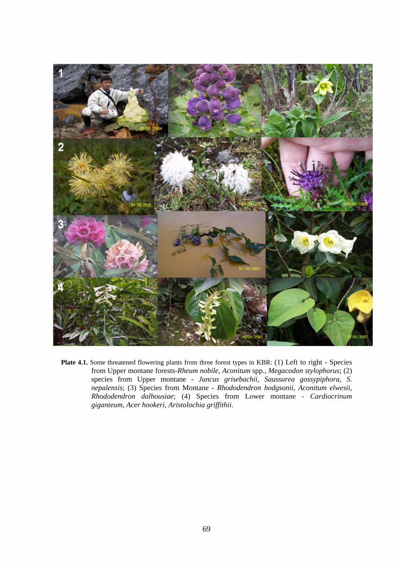
69

Plate 4.1. Some threatened flowering plants from three forest types in KBR: (1) Left to right - Species

from Upper montane forests-Rheum nobile, Aconitum spp., Megacodon stylophorus; (2) species from Upper montane - Juncus grisebachii, Saussurea gossypiphora, S. nepalensis; (3) Species from Montane - Rhododendron hodgsonii, Aconitum elwesii, Rhododendron dalhousiae; (4) Species from Lower montane - Cardiocrinum giganteum, Acer hookeri, Aristolochia griffithii.

70

The variation in α and β-diversity for epiphytes in three forest types may be due to spatial

microhabitats, following a gradient from moist part of the studied forest (LM) to the drier

part (UM) and suggests that the distance to moisture sources plays a crucial role in

determining richness and composition of epiphyte communities. It has also been argued

that epiphyte richness is associated with moisture of the slopes where they grow (Sanford

1968; Sudgen & Robins 1979). β-diversity measures the extent of species replacement or

biotic change along environmental gradients (Whittaker 1972; Brokaw & Scheiner 1989).

It also reflects the extent of similarity and habitat diversity among the forest types. In the

present study, β-diversity for trees and lianas was lower than the shrub and herb

components of the vegetation. The β-diversity values for all the components were

however less than that obtained for BCI forest studied by Brokaw & Scheiner (1989).

Homogeneity in vegetation structure, less diverse microhabitats (Barik et al. 1992) and

availability of less treefall gaps could be the reasons of lower β-diversity in the Eastern

Himalayan forests.

Similarity test for species composition between the three forest types showed that

the forests were significantly dissimilar. It also revealed that the floristic composition had

greater similarity among the adjacent forests and had greater dissimilarity among the

forests located farther apart. Such differences in species composition may be attributed

primarily to the elevational variations (Grell et al. 2005).

As expected, the tree basal area of the Lower montane forests was higher than that

of Montane and Upper montane forests which could be attributed to more number of

individuals in the higher girth classes. The overall tree density-diameter distribution

pattern indicates a rather stable tree population structure in all the three forests (Rao et al.

1990).

The higher value of dominance index for the tree species in Lower montane

forests could be due to increased stress on account of the low disturbance level and

71

extraction of a few trees from the buffer zone of KBR. The low dominance-abundance

curve for lianas as obtained in the Lower montane forests indicated more equitable

resource distribution pattern among the constituent species than those in the Montane and

the Upper montane forests (Crawley 1997). Such equitable resource distribution pattern

might have made the Lower montane forests more species rich in comparison with

Montane and Upper montane forests.

The dominance of the polypodiaceae is a trend in most humid montane epiphyte

communities. Dominance-diversity curves also showed that most IVI was shared by a

few species in the Upper montane forests while in the Montane and the Lower montane

forests, IVI was equitably distributed. The greater dominance pattern in Upper montane

forests indicates that the community is non-equilibrium (Hubbell 1979). Ordination of

forest types on the basis of abundance data with respect to epiphyte species compositions

resulted into slight overlapping of the Montane forests species with the Lower montane

and Montane forests species. The similarities between orchids and fern species are mainly

responsible for this overlapping. The long repent lifeform of Bulbophyllum spp., and

pendant lifeform of Hoya spp., allow plant stems to search for light whilst retaining an

original attachment, an effective local colonisation mechanism. The abundance of this

lifeform was also reported by Freiberg (1996) in montane forest of Ecuador.

The selected host trees for epiphytes ranged from ≥ 35 to < 90 cm diameter. The

occurrence of large number of species on bigger diameter classes can be explained by the

larger area offered with a great variety of host architecture with different microhabitats

(Annaselvam & Parthasarathy 2001). The significant relationship between epiphyte

species and trunk girth class conforms to the findings of Catling and Lefkovitch (1989) in

a Gautemalan forest. The thick humus rich branches and stems are densely covered with

epiphytes, accumulating substantial amount of humus, nutrients and moisture. These are

appropriate requirements as reported in cloud forest of Veracruz, Mexico (Heitz & Hietz-

72

Seifert 1995a) and in West African rain forest (Johansson 1974, 1975). The larger

epiphytes in KBR such as Vaccinium nummularia, Rhododendron dalhousiae, R.

Pendulum in the Montane and Upper montane forests and Macropanax undulatum,

Pentapanax leschenaultii, V. vacciniaceum, Wightia speciosissima, and Drynaria

propinqua in Lower montane forests therefore, inhabit bigger trees such as, Lithocarpus

pachyphylla, Schima wallichii and Elaeocarpus lanceaefolius.

The number and density of epiphytic species increased with increase in height

class of the host tree. Tree tops, branches and twigs together represented a wider range of

the microclimatic gradient, from the more shady environments near the trunk to the

outermost parts of the tree, where exposure to light and desiccating wind were common.

Tree base was poor in epiphytes, only some Araceae inhabited these strata. The richest

trunk vegetation was found on the mossy substratum. This was common in the Upper

montane and Montane forests on Abies densa and Quercus lamellosa host respectively.

The occurrence of more epiphytes in upper canopy layer than any other part of the tree

may be attributed to the bryophyte mats present in larger surface area. The epiphytes also

occupied the forks of tree trunk which accumulate litter and humus and provide

mechanical support. The high canopy dwelling species are Eria coronaria, Dendrobium

spp., Lepisorus spp., Phalaenopsis tainitis, Vittaria spp., and Vaccinium spp. Most of

them are orchids as they are able to withstand drought (Benzing 1976). Long and fine

roots of Orchidaceae also seem adaptive to this special habitat.

Seasonal variation in air temperature, soil temperature, moisture content, C and N

concentrations as observed in the present study corroborates the findings of Barik et al.

(1992) in a subtropical broad-leaved forest of north-east India. However, studies

depicting variation in microenvironmental factors among different forest types are rare. In

addition to elevation, light, soil pH, C, N and P were correlated with abundance data.

Differences in soil properties, elevation, topography and other environmental conditions

73

in different forest types could explain substantially the observed differences in plant

species diversity and abundance in the three forests. An observed gradient in many

environmental variables was also related to the differences in structural and functional

characteristics of the forest types studied along an elevation gradient in Tierra del Fuego

by Frangi et al. (2005).

Relatively lower eigen values of the first two constrained CCA axes and greater

eigen values of the first residual (non canonical) axis as obtained in the present study

apparently indicate that the environmental variables are not sufficient to predict the main

variations on species abundance extracted by CCA, but they do predict a substantial part

of remaining variations. Ter Braak and Prentice (1988) opined that terrestrial community

data commonly give a residual eigen value as large as the first constrained eigen value,

however carefully the environmental variables are chosen. Some of the plant species were

confined to specific forest types while others occurred across the whole range.

The strong clustering of Lower montane trees, shrubs, herbs and lianas along the

soil pH and light gradients in the CCA ordination plot supported the earlier observations

on plant preference for less acidic soil and light (Lowe & Walker 1977; Putz 1984;

Whitmore 1989; Phillips & Gentry 1994). The important role of light in determining the

density and distribution of many liana species such as Cissus repens Clematis acuminata

and Parthenocissus himalayana is in conformity with the findings of Castellanos (1991),

who concluded that liana species thrives well in areas of abundant light in the forest.

Study by Laurance et al. (2001) on the effect of forest fragmentation and treefall gaps on

liana communities concluded that liana abundance increased considerably near forest

edges. However, in the Montane and Upper montane forests, the abundance of trees,

shrubs, herbs and lianas was mainly driven by the edaphic variables (N, P and K). As

shown by stepwise forward multiple regression analysis, light and soil P either alone or

both influenced liana density in different forests. Soil pH in Lower montane and C in

74

Montane and Upper montane forests influenced tree density. Liana and tree desity in the

Montane and Upper montane forests were strongly related to soil nutrients such as N and

P, and pH, C, respectively. Light and C either alone or both influenced shrub density in

Montane and Upper montane forests. pH, elevation in the Montane, N and P either alone

or both influenced herb density in Montane and Upper montane forests respectively. The

role of soil nutrients in plant species distribution was emphasised by Dewalt et al. (2000,

2006) and Godefroid et al. (2007) corroborating to the present finding. All these abiotic

factors influence the adaptation and survival of the plant species contributing to greater

species diversity in the forest communities (Ibarra-Manríquez & Martínez-Ramos 2004;

van der Heijden & Phillips 2008).

Epiphytic species had strong clustering around RH, elevations and air

temperature. Result of stepwise forward multiple regression analysis also showed the

influence of light, elevation and relative humidity on epiphyte density. The roles of

elevational gradient and RH in epiphyte richness were also emphasised by Kufer et al.

(2004), and Kharkwal et al. (2005) corroborating to the present finding. Upto 107

epiphyte species were reported by Valdivia (1977) on a single tree where dense evergreen

canopies feature multiple microclimates and numerous alternatives to earth soil. He

attributed such high species richness to relative humidity. But many epiphytes require

high exposure and others like certain filmy ferns cannot endure either as much light or the

associated aridity (Hietz & Briones 1998). Consequently, epiphytes segregated along the

environmental gradients in different forest types (Annexure 2).

To conclude, it is evident that there are considerable differences in species

composition among different forests types. This was attributed to diversity in hahitat

types, forest types, host structure, and available environmental and forest structural

gradients.

86

Annexure 1. Density (ind ha-1), basal area (m2 ha-1) and IVI of trees, shrubs and herbs in three forest types. Name of species Lower montane Montane Upper montane

Family Den. IVI BA Den. IVI BA Den. IVI BA

Trees

Abies densa Griffith. Pinaceae - - - - - - 37.50 67.41 0.28

Acer campbellii Hk. f. & Thoms ex Hiern. Aceraceae 10.00 6.39 0.06 - - - - - -

Acer spp. Aceraceae - - - 6.00 7.24 0.09 - - -

Acer thomsonii Miq. Aceraceae - - - 3.50 4.11 0.09 - - -

Alangium alpinum (Clarke) Sm. & Cave Alangiaceae - - - 5.00 6.95 0.11 - - -

Alangium begoniaefolium Baill. Alangiaceae - - - 6.00 6.18 0.04 - - -

Albizia chinensis (Osbeck.F) Merr. Fabaceae 9.00 5.34 0.06 - - - - - -

Alnus nepalensis D. Don Betulaceae 29.00 23.86 0.19 5.50 4.51 0.04 - - -

Betula alnoides Buch. - Ham. ex D. Don Betulaceae - - - 10.50 14.66 0.13 - - -

Buddleja colvilei Thom. Buddlejaceae - - - - - - 11.50 12.02 0.05

Castanopsis hystrix A. DC. Fagaceae 14.00 14.48 0.28 - - - - - -

Castanopsis indica (Roxb ex Lindl.) A.DC. Fagaceae 6.00 5.59 0.22 - - - - - -

Castanopsis tribuloides (Sm.) A. DC. Fagaceae 10.00 10.95 0.31 - - - - - -

Cinnamomum bejolghota (Buch. – Ham.) Sweet Lauraceae 8.00 4.90 0.06 - - - - - -

Cinnamomum impressinervium Meisn. Lauraceae 4.50 2.75 0.04 9.50 14.25 0.17 - - -

Daphne bholua Buch. – Ham. ex D. Don Thymelaceae - - - 7.50 7.37 0.05 - - -

Daphne papyracea Wall. ex Steud Thymelaceae 7.00 3.40 0.03 - - - - - -

Dendrocalamus hamiltonii Nees et Arn. ex Munro Poaceae 11.00 5.43 0.04 - - - - - -

Elaeocarpus lanceaefolius Roxb. Elaeocarpaceae 24.00 19.61 0.18 6.50 6.25 0.03 - - -

Engelhardtia colebrokiana Lindl. Juglandaceae 8.00 4.66 0.09 - - - - - -

Engelhardtia spicata Lesch ex Bl. Juglandaceae 8.00 6.47 0.15 - - - - - -

Euodia fraxinifolia Hk. f. Theaceae 20.00 10.99 0.06 10.50 14.33 0.13 - - -

Eurya cerasifolia (D. Don) Kobuski Theaceae 16.00 8.59 0.06 - - - - - -

87

Eurya japonica Thunb. Theaceae 10.50 6.03 0.09 4.00 6.11 0.07 - - -

Exbucklandia populnea (R. Br ex Griff.) R. Br. Hamamelidaceae 9.00 8.03 0.22 - - - - - -

Ficus auriculata Lour. Moraceae 8.50 4.34 0.04 - - - - - -

Ficus neriifolia Sm. Moraceae 6.00 2.80 0.03 - - - - - -

Ficus semicordata Buch. - Ham ex Sm. Moraceae 6.50 3.45 0.04 - - - - - -

Glochidion acuminatum Mull. Euphorbiaceae 6.50 3.27 0.06 - - - - - -

Hydrangea aspera Buch. - Ham. ex D. Don Hydrangeaceae - - - 7.50 7.87 0.05 - - -

Ilex dipyrena Aquifoliaceae - - - - - - 7.00 11.22 0.09

Ilex fragilis Hk. f. Aquifoliaceae - - - 7.50 6.85 0.04 - - -

Indigofera dosua Buch. - Ham. ex D. Don. Fabaceae 3.00 1.53 0.03 - - - - - -

Juglans regia L. Juglandaceae 17.00 13.34 0.17 - - - - - -

Leucosceptrum canum Sm. Lamiaceae 7.00 4.00 0.07 8.50 9.82 0.09 - - -

Lithocarpus elegans (Bl.) Hatus ex Soepadmo Fagaceae 6.00 5.85 0.27 - - - - - -

Lithocarpus pachyphylla (Kurz) Rehder Fagaceae - - - 6.50 6.72 0.08 - - -

Litsea cubeba Bl. Lauraceae 9.00 5.43 0.07 - - - - - -

Litsea elongata (Wall. ex Nees.) Benth. et Hk. f. Lauraceae - - - 15.50 23.70 0.18 - - -

Lyonia ovalifolia (Wall.) Drude Ericaceae 11.50 5.43 0.05 11.00 12.29 0.07 - - -

Macaranga denticulata (Bl.) Muell. – Arg. Euphorbiaceae 12.00 6.32 0.06 - - - - - -

Macaranga indica Wight Euphorbiaceae 6.50 3.27 0.06 - - - - - -

Macaranga pustulata King ex Hk. f. Euphorbiaceae 14.00 7.03 0.06 - - - - - -

Magnolia campbellii Hk. f. & Thoms. Magnoliaceae - - - 9.50 9.53 0.08 - - -

Myrsine semiserrata Wall. Myrsinaceae 15.00 7.97 0.04 - - - - - -

Pentapanax leschenaultii (DC.) Seem. Araliaceae 4.50 2.36 0.03 - - - - - -

Persea gammieana Kosterm. ex Kosterm. & Charter Lauraceae - - - 12.00 21.40 0.24 - - -

Prunus cerasoides D. Don Rosaceae 7.00 3.76 0.05 - - - - - -

Prunus cornuta (Royle) Steud. Rosaceae - - - 7.00 10.44 0.10 - - -

Prunus spp. Rosaceae - - - - - - 18.00 17.14 0.08

Quercus lamellosa Sm. Fagaceae - - - 9.50 8.33 0.06 - - -

88

Quercus lineata Bl. Fagaceae 12.00 13.84 0.32 7.50 15.78 0.24 - - -

Rhododendron arboreum Sm. Ericaceae - - - 8.00 15.72 0.22 - - -

Rhododendron campanulatum D. Don Ericaceae - - - - - - 45.00 36.11 0.05

Rhododendron cinnabarinumHook.f. Ericaceae - - - - - - 13.00 8.45 0.04

Rhododendron falconeri Hk. f. Ericaceae - - - 17.50 18.70 0.09 17.50 13.97 0.06

Rhododendron grande Wight Ericaceae - - - - - - 28.50 39.79 0.06

Rhododendron thomsonii Hk. f. Ericaceae - - - - - - 20.50 17.26 0.03

Rhododendrum spp. Sm. Ericaceae - - - - - - 42.50 38.00 0.09

Rhus hookeri Sahni & Bahadur Anacardiaceae 1.50 1.35 0.09 - - - - - -

Rhus javanica Hk. f. Anacardiaceae 13.00 7.46 0.04 - - - - - -

Ricinus communis L. Euphorbiaceae 13.00 6.34 0.02 - - - - - -

Saurauia napaulensis DC. Saurauiaceae 3.00 1.66 0.05 - - - - - -

Schefflera impressa (Clarke) Harms Araliaceae 6.50 3.15 0.02 - - - - - -

Symplocos glomerata King ex Gamble Symplocaceae 5.50 3.72 0.03 - - - - - -

Symplocos ramosissima Wall. ex D. Don Symplocaceae - - - 13.00 15.00 0.09 - - -

Symplocos theifolia D. Don Symplocaceae - - - 6.00 6.73 0.07 - - -

Talauma hodgsonii Hk. f. & Thoms. Magnoliaceae 3.00 2.64 0.14 - - - - - -

Toona ciliata M. Roem. Anacardiaceae 4.50 3.86 0.15 - - - - - -

Toricellia tillifolia DC. Toricelliaceae 13.50 6.24 0.04 - - - - - -

Trevesia palmata (Roxb.) Vis. Araliaceae 3.00 1.59 0.03 - - - - - -

Tsuga dumosa (D. Don) Eichler Pinaceae - - - - - - 24.00 38.64 0.27

Viburnum cylindricum Buch. - Ham. ex D. Don Caprifoliaceae 14.00 6.65 0.03 - - - - - -

Viburnum mullaha Buch. - Ham. ex D. Don Caprifoliaceae 6.00 3.08 0.03 - - - - - -

Viburnum nervosum D. Don Caprifoliacea 7.00 3.43 0.03 6.50 8.98 0.06 - - -

Wendlandia paniculata DC. Rubiaceae 6.00 3.51 0.06 - - - - - -

Zanthoxylum oxyphyllumEdgew Rutaceae 7.50 3.90 0.03 11.50 10.16 0.03 - - -


Shrub Family Den. IVI Den. IVI Den. IVI

89

Aconogonum molle (D. Don) Hara Polygonaceae 8.00 4.56 - - - -

Arundinaria maling Gamble Poaceae - - 21.50 29.182 - -

Bambusa nutans Wall. ex Munro Poaceae 20.00 8.32 - - - -

Berberis sikkimensis Ahrendt Berberidaceae - - 25.00 37.91 - -

Berberis spp. Berberidaceae - - - - 40 37.094

Boehmeria macrophylla D. Don Urticaceae 7.50 4.41 - - - -

Boehmeria platyphylla D. Don Urticaceae 17.00 9.44 - - - -

Clerodendron colebrookianum Walp. Verbenaceae 7.00 6.30 - - - -

Daphne bholua Buch. - Ham. ex D. Don Thymelaceae 7.00 4.93 - - - -

Debregeasia longifolia (Burm. f.) Wedd. Urticaceae 10.00 6.56 - - - -

Desmodium confertum DC. Fabaceae 5.00 4.31 - - - -

Deutzia compacta Craib Hydrangeaceae - - 14.00 29.651 - -

Dichroa febrifuga Lour. Hydrangeaceae 6.50 4.09 - - - -

Dicranopteris linearis (Burm. f.) Underw. Gleicheniaceae 18.50 7.17 - - - -

Dobinea vulgaris Buch. - Ham. ex D. Don Rubiaceae 12.50 8.03 - - - -

Edgeworthia gardneri (Wall.) Meisn. Thymelaceae 7.00 4.93 8.50 21.574 - -

Elsholtzia flava (Benth.) Benth. Lamiaceae 30.00 13.51 - - - -

Girardina diversifolia (Link) Friis Urticaceae 9.50 5.03 - - - -

Gleichenia glauca (Thunb.) Hook. Gleicheniaceae 11.00 4.82 - - - -

Juniperus recurva Buch. – Ham. ex D. Don Cupressaceae - - - - 29.50 29.75

Luculia gratissima (Wall.) Meisn. Rubiaceae 18.00 12.49 - - - -

Maesa chisia Buch. - Ham ex D.Don Myrsinaceae 9.00 4.19 - - - -

Maesa ramentacea Wall. ex Roxb.. Myrsinaceae 8.00 5.93 - - - -

Melastoma malabathricum L. Melastomatacae 9.00 6.93 - - - -

Melastoma normale D. Don Melastomataceae 13.00 9.55 - - - -

Mussaenda treutleri Stapf. Rubiaceae 10.00 5.87 - - - -

Neillia rubiflora D. Don Rosaceae 7.00 6.30 - - - -

Osbeckia sikkimensis Craib. Melastomataceae 2.00 2.00 - - - -

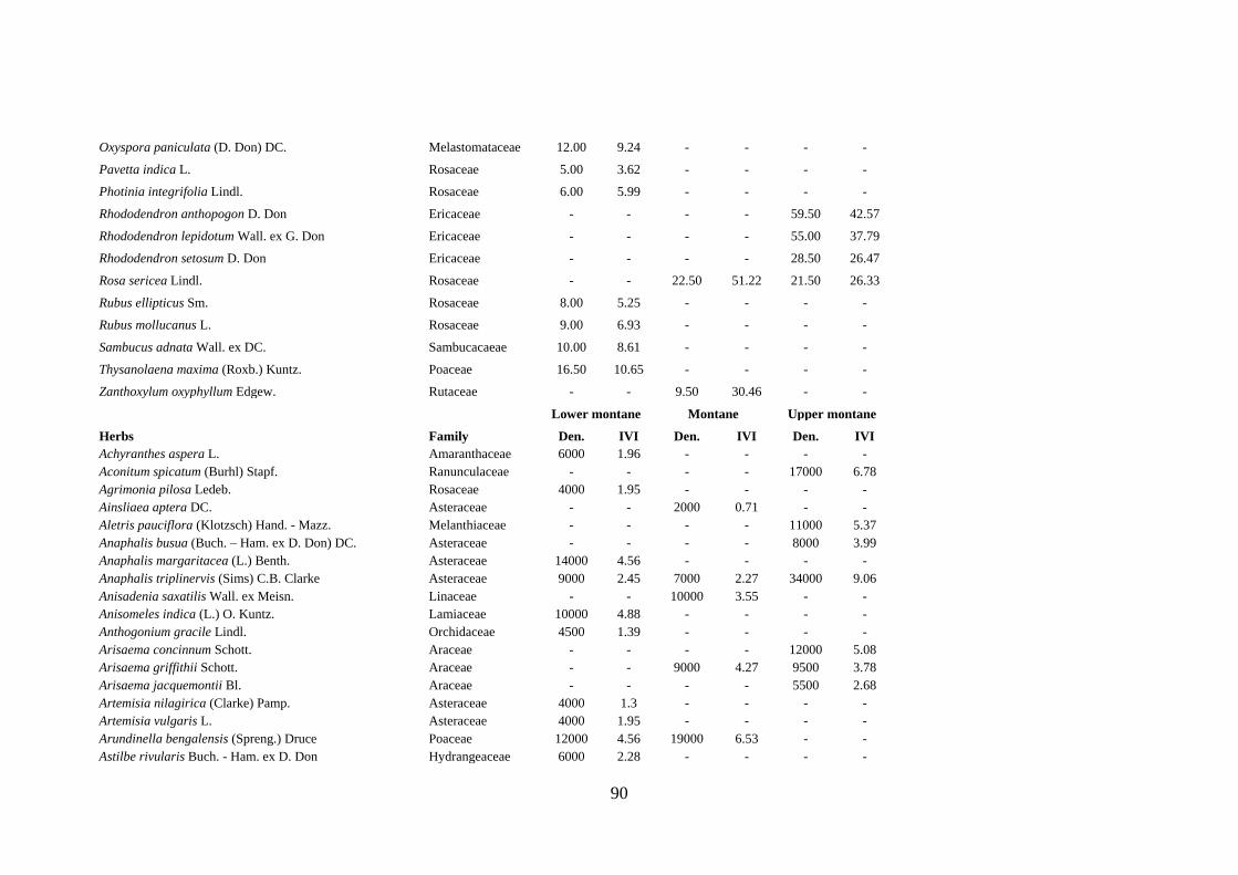
90

Oxyspora paniculata (D. Don) DC. Melastomataceae 12.00 9.24 - - - -

Pavetta indica L. Rosaceae 5.00 3.62 - - - -

Photinia integrifolia Lindl. Rosaceae 6.00 5.99 - - - -

Rhododendron anthopogon D. Don Ericaceae - - - - 59.50 42.57

Rhododendron lepidotum Wall. ex G. Don Ericaceae - - - - 55.00 37.79

Rhododendron setosum D. Don Ericaceae - - - - 28.50 26.47

Rosa sericea Lindl. Rosaceae - - 22.50 51.22 21.50 26.33

Rubus ellipticus Sm. Rosaceae 8.00 5.25 - - - -

Rubus mollucanus L. Rosaceae 9.00 6.93 - - - -

Sambucus adnata Wall. ex DC. Sambucacaeae 10.00 8.61 - - - -

Thysanolaena maxima (Roxb.) Kuntz. Poaceae 16.50 10.65 - - - -

Zanthoxylum oxyphyllum Edgew. Rutaceae - - 9.50 30.46 - -


Herbs Family Den. IVI Den. IVI Den. IVI Achyranthes aspera L. Amaranthaceae 6000 1.96 - - - - Aconitum spicatum (Burhl) Stapf. Ranunculaceae - - - - 17000 6.78 Agrimonia pilosa Ledeb. Rosaceae 4000 1.95 - - - - Ainsliaea aptera DC. Asteraceae - - 2000 0.71 - - Aletris pauciflora (Klotzsch) Hand. - Mazz. Melanthiaceae - - - - 11000 5.37 Anaphalis busua (Buch. – Ham. ex D. Don) DC. Asteraceae - - - - 8000 3.99 Anaphalis margaritacea (L.) Benth. Asteraceae 14000 4.56 - - - - Anaphalis triplinervis (Sims) C.B. Clarke Asteraceae 9000 2.45 7000 2.27 34000 9.06 Anisadenia saxatilis Wall. ex Meisn. Linaceae - - 10000 3.55 - - Anisomeles indica (L.) O. Kuntz. Lamiaceae 10000 4.88 - - - - Anthogonium gracile Lindl. Orchidaceae 4500 1.39 - - - - Arisaema concinnum Schott. Araceae - - - - 12000 5.08 Arisaema griffithii Schott. Araceae - - 9000 4.27 9500 3.78 Arisaema jacquemontii Bl. Araceae - - - - 5500 2.68 Artemisia nilagirica (Clarke) Pamp. Asteraceae 4000 1.3 - - - - Artemisia vulgaris L. Asteraceae 4000 1.95 - - - - Arundinella bengalensis (Spreng.) Druce Poaceae 12000 4.56 19000 6.53 - - Astilbe rivularis Buch. - Ham. ex D. Don Hydrangeaceae 6000 2.28 - - - -

91

Athyrium rubricaule (Edgew. ex C. B. Clarke) Bir Athyriaceae 2000 0.98 6000 2.56 - - Begonia josephii DC. Begoniaceae - - - - 11000 4.47 Begonia rubella Buch. - Ham. ex D. Don Begoniaceae 4000 1.95 - - - - Bidens biternata (Lour.) Merr. & Sherff. Asteraceae 28000 5.89 - - - - Bidens pilosa L. Asteraceae 19000 7.65 - - - - Bistorta affinis (D. Don) Greene Polygonaceae - - - - 11000 4.02 Bupleurum longicaule Wall. ex DC. Apiaceae - - - - 6500 3.30 Caltha palustris L. Ranunculaceae - - - - 5000 2.15 Campanula pallida Wall. Campanulaceae 14000 5.53 - - - - Campylandra aurantiaca Baker Liliaceae - - 17500 3.75 - - Carex filicina Nees Cyperaceae 22000 6.85 - - - - Cautleya gracilis (Sm.) Dandy Zingiberaceae 7500 2.53 - - - - Chlorophytum nepalense (Lindl.) Baker Anthericaceae 13500 5.45 - - - - Chrysosplenium carnosum Hk. f. & Thoms. Saxifragaceae - - 17000 6.25 - - Cirsium verutum (D. Don) Spreng. Asteraceae - - - - 7500 3.46 Clintonia udensis Trautv. & Mey. Liliaceae - - - - 12500 3.81 Coniogramme cautata (Wall. ex Ettingshausen) Ching Hemionitidaceae 6000 2.93 - - - - Craniotome furcata (Link) Kuntz. Lamiaceae - - 23500 3.73 - - Cuphea balsamona Cham. et Schlechtend Lythraceae 7000 3.09 - - - - Cyanotis vaga (Lour.) Schult. & Schult. f. Commelinaceae 12000 5.21 36500 8.56 - - Cyathula capitata Miq. Lamiaceae - - 25000 5.23 - - Cynodon dactylon (L.) Pers. Poaceae 21500 4.17 - - - - Cyperus niveus Retz. Cyperaceae - - 4000 1.42 - - Cyperus rotundus L. Cyperaceae 4000 1.42 5000 1.99 - - Desmodium multiflorum DC. Fabaceae 10000 4.88 - - - - Dicrocephala integrifolia (Lf) Kuntz. Asteraceae 11000 3.75 - - - - Dryopteris barbigera (Hk.) O. Kuntz.) Dryopteridaceae 12000 4.56 20500 5.03 - - Dryopteris chrysocoma (Christ.) C. Chr. Dryopteridaceae 8000 3.9 - - - - Dryopteris sparsa (D. Don) O. Kuntz. Dryopteridaceae 6000 2.93 - - - - Dryopteris spp. Dryopteridaceae - - - - 16000 7.07 Elatostema obtusum Wedd. Urticaceae - - 4000 1.42 - - Elatostemma platyphylla Wedd. Urticaceae - - 6000 2.56 - - Elatostemma sessile J. R. & G. Forst. Urticaceae - - 17500 5.89 - - Elsholtzia blanda (Benth.) Benth. Lamiaceae 24000 7.17 - - - - Elsholtzia fruticosa (D. Don) Rehder Lamiaceae - - 11000 3.26 - -

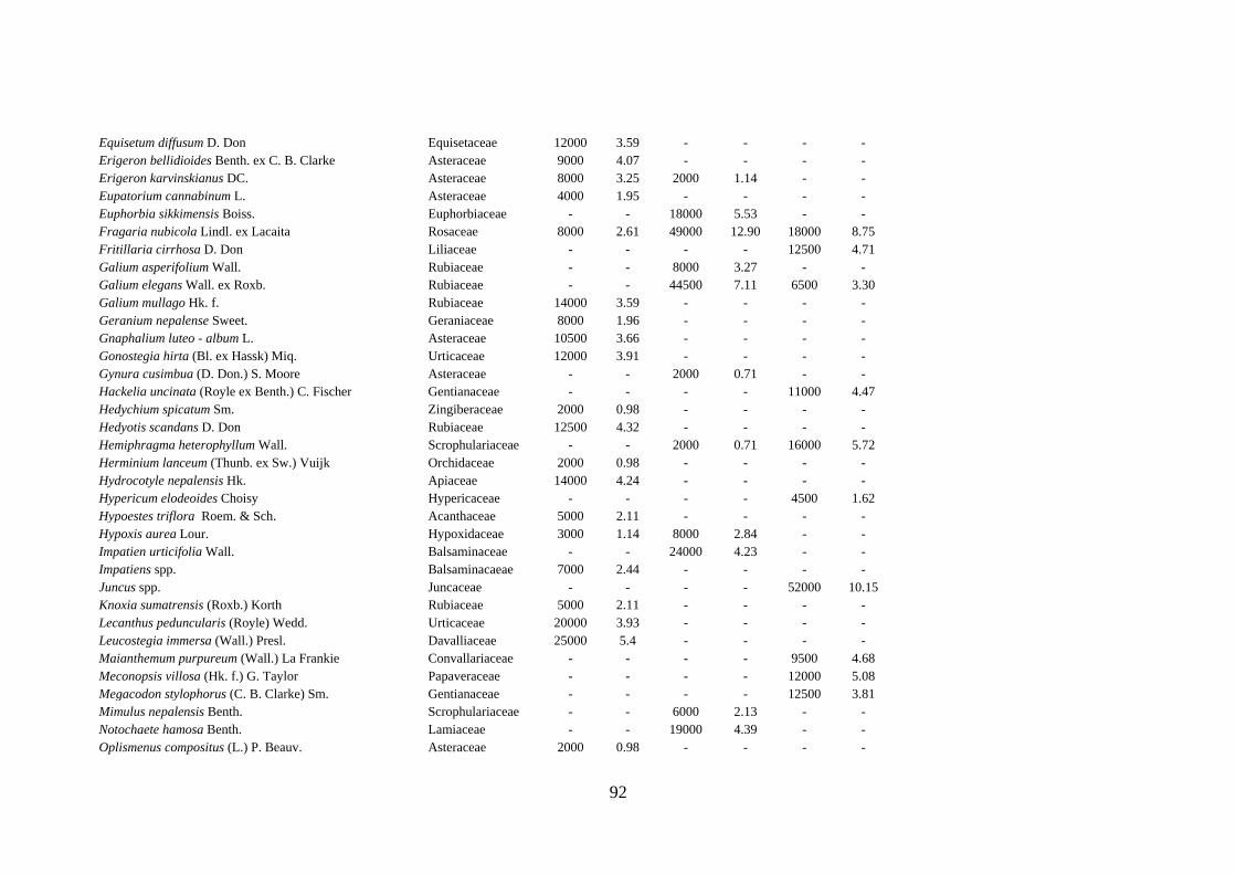
92

Equisetum diffusum D. Don Equisetaceae 12000 3.59 - - - - Erigeron bellidioides Benth. ex C. B. Clarke Asteraceae 9000 4.07 - - - - Erigeron karvinskianus DC. Asteraceae 8000 3.25 2000 1.14 - - Eupatorium cannabinum L. Asteraceae 4000 1.95 - - - - Euphorbia sikkimensis Boiss. Euphorbiaceae - - 18000 5.53 - - Fragaria nubicola Lindl. ex Lacaita Rosaceae 8000 2.61 49000 12.90 18000 8.75 Fritillaria cirrhosa D. Don Liliaceae - - - - 12500 4.71 Galium asperifolium Wall. Rubiaceae - - 8000 3.27 - - Galium elegans Wall. ex Roxb. Rubiaceae - - 44500 7.11 6500 3.30 Galium mullago Hk. f. Rubiaceae 14000 3.59 - - - - Geranium nepalense Sweet. Geraniaceae 8000 1.96 - - - - Gnaphalium luteo - album L. Asteraceae 10500 3.66 - - - - Gonostegia hirta (Bl. ex Hassk) Miq. Urticaceae 12000 3.91 - - - - Gynura cusimbua (D. Don.) S. Moore Asteraceae - - 2000 0.71 - - Hackelia uncinata (Royle ex Benth.) C. Fischer Gentianaceae - - - - 11000 4.47 Hedychium spicatum Sm. Zingiberaceae 2000 0.98 - - - - Hedyotis scandans D. Don Rubiaceae 12500 4.32 - - - - Hemiphragma heterophyllum Wall. Scrophulariaceae - - 2000 0.71 16000 5.72 Herminium lanceum (Thunb. ex Sw.) Vuijk Orchidaceae 2000 0.98 - - - - Hydrocotyle nepalensis Hk. Apiaceae 14000 4.24 - - - - Hypericum elodeoides Choisy Hypericaceae - - - - 4500 1.62 Hypoestes triflora Roem. & Sch. Acanthaceae 5000 2.11 - - - - Hypoxis aurea Lour. Hypoxidaceae 3000 1.14 8000 2.84 - - Impatien urticifolia Wall. Balsaminaceae - - 24000 4.23 - - Impatiens spp. Balsaminacaeae 7000 2.44 - - - - Juncus spp. Juncaceae - - - - 52000 10.15 Knoxia sumatrensis (Roxb.) Korth Rubiaceae 5000 2.11 - - - - Lecanthus peduncularis (Royle) Wedd. Urticaceae 20000 3.93 - - - - Leucostegia immersa (Wall.) Presl. Davalliaceae 25000 5.4 - - - - Maianthemum purpureum (Wall.) La Frankie Convallariaceae - - - - 9500 4.68 Meconopsis villosa (Hk. f.) G. Taylor Papaveraceae - - - - 12000 5.08 Megacodon stylophorus (C. B. Clarke) Sm. Gentianaceae - - - - 12500 3.81 Mimulus nepalensis Benth. Scrophulariaceae - - 6000 2.13 - - Notochaete hamosa Benth. Lamiaceae - - 19000 4.39 - - Oplismenus compositus (L.) P. Beauv. Asteraceae 2000 0.98 - - - -

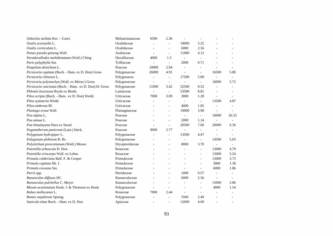
93

Osbeckia stellata Ker. – Gawl. Melastomataceae 6500 2.36 - - - - Oxalis acetosella L. Oxalidaceae - - 19000 5.25 - - Oxalis corniculata L. Oxalidaceae - - 6000 2.56 - - Panax pseudo ginseng Wall. Araliaceae - - 11000 4.12 - - Paradavallodes multidentatum (Wall.) Ching Davalliaceae 4000 1.3 - - - - Paris polyphylla Sm. Trilliaceae - - 2000 0.71 - - Paspalum destichum L. Poaceae 10000 2.94 - - - - Persicaria capitata (Buch. - Ham. ex D. Don) Gross Polygonaceae 26000 4.91 - - 16500 5.80 Persicaria chinense L. Polygonacea - - 17500 5.89 - - Persicaria polystachya (Wall. ex Meisn.) Gross Polygonaceae - - - - 16000 5.72 Persicaria runcinata (Buch. - Ham. ex D. Don) H. Gross Polygonaceae 11000 3.42 52500 9.52 - - Phlomis bracteosa Royle ex Benth. Lamiaceae - - 53500 8.81 - - Pilea scripta (Buch. - Ham. ex D. Don) Wedd. Urticaceae 7000 3.09 3000 1.28 - - Pilea symmeria Wedd. Urticaceae - - - - 13500 4.87 Pilea umbrosa Bl. Urticaceae - - 4000 1.85 - - Plantago erosa Wall. Plantaginaceae - - 10000 3.98 - - Poa alpina L. Poaceae - - - - 16000 26.33 Poa annua L. Poaceae - - 2000 1.14 - - Poa himalayana Nees ex Steud. Poaceae - - 20500 7.60 20000 6.36 Pogonatherum paniceum (Lam.) Hack. Poaceae 9000 2.77 - - - - Polygonum hydropiper L. Polygonaceae - - 13500 4.47 - - Polygonum plebeium R. Br. Polygonaceae - - - - 14500 5.03 Polystichum prescotianum (Wall.) Moore. Dryopteridaceae - - 8000 3.70 - - Potentilla arbuscula D. Don. Rosaceae - - - - 13000 4.79 Potentilla eriocarpa Wall. ex Lehm. Rosaceae - - - - 13000 5.24 Primula calderiana Balf. F. & Cooper Primulaceae - - - - 12000 3.73 Primula capitata Hk. f. Primulaceae - - - - 3000 1.38 Primula caveana Sm. Primulaceae - - - - 6000 1.86 Pteris spp. Pteridaceae - - 1000 0.57 - - Ranunculus diffusus DC. Ranunculaceae - - 6000 2.56 - - Ranunculus pulchellus C. Meyer Ranunculaceae - - - - 15000 2.86 Rheum acuminatum Hook. f. & Thomson ex Hook. Polygonaceae - - - - 4000 1.54 Rubus mollucanus L. Rosaceae 7000 2.44 - - - - Rumex nepalensis Spreng. Polygonaceae - - 5500 2.49 - - Sanicula elata Buch. - Ham. ex D. Don Apiaceae - - 12000 4.69 - -

94

Scoparia dulcis DC. Scrophulariaceae 3000 1.14 - - - - Selenium tenuifolium Wall. ex C. B. Clarke Apiaceae - - - - 12000 3.73 Senecio diversifolius Wall. ex DC. Asteraceae - - - - 7500 3.46 Senecio wallichii DC. Asteraceae - - 6500 3.06 - - Spilanthes paniculatus Wall. ex DC. Asteraceae 13000 2.46 - - - - Stellaria sikkimensis Hk. f. Edgew. & Hk. f. Caryophyllaceae - - 8500 2.91 - - Swertia chirayita (Roxb. ex Flem.) Karst. Gentianaceae 9000 2.77 - - - - Urtica dioica L. Urticaceae - - 8000 2.84 - - Valeriana hardwickii Wall. Valerianaceae 14000 4.56 - - - - Viola biflora L. Violaceae - - 14500 4.61 - - Viola pilosa Bl. Violaceae 6000 1.96 - - - -

86

Annexure 2. Frequency, density (tree-1) and IVI of epiphytes in three forest stands.

Upper montane Montane Lower montane

Epiphytes Family Frequency Density

tree-1 IVI Frequency Density tree-1 IVI Frequency

Density tree-1 IVI

Aeschynanthus bracteatus Wall. ex DC. Gesneriaceae - - - 10 20 1.73 10 20 1.51 Aeschynanthus hookeri Clarke Gesneeriaceae - - - - - - 20 40 3.02 Aeschynanthus sikkimensis (Clarke) Stapf Gesneriaceae - - - - - - 10 20 1.51 Agapetes hookeri(Clarke) Sleumer Ericaceae - - - 10 50 2.35 10 20 1.51 Agapetes incurvata (Griff.) Sleumer Ericaceae - - - 10 20 1.73 - - - Agapetes serpens (Wight) Sleumer Ericaceae - - - - - - 10 70 2.47 Agrostophyllum brevipes King & Pantl. Orchidaceae - - - - - - 10 10 1.32 Agrostophyllum callosum Rchb. f. Orchidaceae - - - - - - 10 20 1.51 Arthomeris himalayensis (Hk.) Ching Polypodiaceae 20 60 7.06 - - - - - - Arthomeris lehmanii (Mett.) Ching Polypodiaceae - - - 10 30 1.94 - - - Arthomeris wallichiana (Spr.) Ching Polypodiaceae 10 40 3.95 10 30 1.94 - - - Asplenium ensiforme Wall. Aspleniaceae - - - 10 20 1.73 - - - Belvisia spicata (L.f.) Mirbel Polypodiaceae - - - - - - 10 110 3.24 Bulbophyllum cauliflorum Hk.f. Orchidaceae - - - - - - 10 20 1.51 Bulbophyllum reptans (lindl.) Lindl. Orchidaceae - - - 10 40 2.14 10 50 2.09 Cautleya gracilis(Smith) Dandy Zingiberaceae - - - 10 50 2.35 10 70 2.47 Cheilanthes formosana Hay. Sinopteridaceae - - - 10 20 1.73 - - - Codonopsis purpurea Wall. Campanulaceae - - - 10 20 1.73 - - - Coelogynae corymbosa Lindl. Orchidaceae - - - 30 30 4.57 20 30 2.82 Coelogynae ochracea Lindl. Orchidaceae - - - 10 20 1.73 - - - Cystopteris sudetica A. Br. Davalliaceae 70 340 30.14 - - - - - - Davallia bullata Wall. Davalliaceae - - - - - - 10 20 1.51 Dendrobium amoenum Wall. ex Lindl. Orchidaceae - - - - - - 10 20 1.51 Dendrobium longicornu Lindl. Orchidaceae - - - - - - 10 10 1.32 Dendrobium nobile Lindl. Orchidaceae - - - - - - 10 10 1.32 Didymocarpus aromaticus Wall. ex D. Don Gesneriaceae - - - 20 50 3.67 - - - Didymocarpus oblongus Wall. ex D.Don Gesneeriaceae - - - - - - 20 80 3.79 Drynaria propinqua (Wall.) J. Smith Drynariaceae - - - - - - 10 20 1.51 Eria coronaria (Lindl.) Reichb.f. Orchidaceae - - - - - - 10 10 1.32 Eria spicata (D. Don) Hand. - Mazz. Orchidaceae - - - - - - 10 10 1.32

87

Ficus spp. Moraceae - - - - - - 10 10 1.32 Globba hookeri Clarke ex Baker Zingiberaceae - - - 10 50 2.35 10 70 2.47 Gonatanthus pumilus (D. Don) Engler & Krause Araceae - - - - - - 10 40 1.89 Hoya fusca Wall. Asclepiadaceae - - - - - - 10 30 1.70 Hoya lanceolata Wall. ex D. Don Asclepiadaceae - - - - - - 20 40 3.02 Hoya linearis Wall. ex D. Don Asclepiadaceae - - - 10 310 7.73 60 1120 28.28 Hymenopogon parasiticus Wall. Rubiaceae - - - 10 40 2.14 - - - Lepisorus kashyapii (Mehra) Mehra Polypodiaceae 10 60 4.78 20 140 5.53 20 220 6.48 Lepisorus nudus (Mehra) Mehra Polypodiaceae 30 60 9.33 50 440 15.69 60 580 17.90 Lepisorus scolopendrinus (Don) Mehra & Bir Polypodiaceae 10 20 3.11 30 190 7.88 - - - Lepisorus sesquipedalis (J. Sm.) Fras. - Jenk. Polypodiaceae 10 30 3.53 - - - - - - Leucostegia immersa (Wall.) Presl Davalliaceae - - - - - - 10 60 2.28 Lindsaea odorataRoxb. ex Griff. Lindsaeaceae - - - - - - 10 20 1.51 Lipparis perpusilla Hk. f. Orchidaceae - - - - - - 10 30 1.70 Loxogramme involuta (D. Don) Presl. Loxogrammaceae - - - 10 230 6.08 - - - Lycopodium japonicumThunb. Lycopodiaceae - - - - - - 10 50 2.09 Lysionotus serratus D. Don Gesneriaceae - - - 10 30 1.94 - - - Macropanax undulatum Seem. Araliaceae - - - 10 40 2.14 - - - Mecodium spp. Hymenophyllaceae - - - 30 180 7.67 30 90 5.10 Medinilla himalayana Hk.f Melastomataceae - - - - - - 10 10 1.32 Microsorium membranaceum (D. Don) Ching Polypodiaceae - - - - - - 10 10 1.32 Microsorium punctatum (Linn.) Copel. Polypodiaceae - - - - - - 10 10 1.32 Nephrolepis cordifolia (L.) Presl. Nephrolepidaceae - - - 10 20 1.73 30 80 4.91 Oleandra wallichii (Hk.) Presl. Oleandraceae 30 90 10.58 30 120 6.43 - - - Onychium spp. Cryptogrammaceae 50 670 39.40 - - - - - - Otochilus alba Lindl. Orchidaceae - - - - - - 10 10 1.32 Pentapanax leschenaultii Seem. Araliaceae - - - - - - 10 10 1.32 Pentapanax racemosus Seem. Araliaceae - - - 10 10 1.52 - - - Peperomia heyneana Miquel. Piperaceae - - - - - - 10 70 2.47 Peperomia tetraphylla (Forst. f.) Hk. & Arn. Piperaceae - - - - - - 30 310 9.33 Phalaenopsis tainitis Christenson & Pradhan Orchidaceae - - - - - - 10 40 1.89 Phlegmariurus phlegmaria (L.) Sen.et Sen Huperziaceae - - - - - - 10 10 1.32 Pholidota imbricata Hk. Orchidaceae - - - 10 30 1.94 20 40 3.02 Phymatopteris ebinipes (Hk.) Ching Polypodiaceae 10 30 3.53 - - - - - - Phymatopteris malacodon (Hk.) Pichi - Serm. Polypodiaceae - - - - - - 10 50 2.09

88

Phymatopteris oxyloba (Wall. ex Ktze) Pic. Ser polypodiaceae 50 120 16.38 - - - - - - Pilea spp. Urticaceae 20 60 7.06 10 40 2.14 - - - Pleione hookeriana (Lindl.) O. Kuntze. Orchidaceae - - - 20 200 6.77 - - - Pleione humilis (Smith) D. Don Orchidaceae - - - - - - 20 180 5.71 Polypodiastrum argutum (Wall. ex Hk.) Ching Polypodiaceae 30 370 22.30 40 780 21.41 10 220 5.35 Polypodioides amoena Wall. Polypodiaceae - - - 10 10 1.52 - - - Polypodioides lachnopus Wall. Polypodiaceae - - - 20 80 4.29 10 20 1.51 Pyrrosia flocculosa (D. Don) Ching Polypodiaceae 10 20 3.11 - - - - - - Pyrrosia lanceolata (L.) Farwell Polypodiaceae - - - - - - 20 100 4.17 Pyrrosia stigmosa (Sw.) Ching Polypodiaceae - - - - - - 10 210 5.16 Remusatia hookeriana Schott Araceae - - - - - - 10 70 2.47 Rhododendron dalhousiae Hk. f. Ericaceae - - - - - - 10 20 1.51 Rhododendron pendulum Hk. f. Ericaceae - - - 20 50 3.67 - - - Roscoea spicata Seem. Zingiberaceae 10 20 3.11 20 30 3.25 10 10 1.32 Selaginella spp. Selaginellaceae - - - - - - 10 30 1.70 Smilacina oleracea (Baker) Hk. f. Convallariaceae 10 60 4.78 10 210 5.66 - - - Utricularia multicaulis Oliver Lentibulariaceae - - - 10 20 1.73 - - - Vaccinium nummularia Hk. f. & Thoms. ex Clarke

Ericaceae - - - 10 130 4.01 - - -

Vaccinium retusum (Griffith) Hoo. f. ex Clarke Ericaceae 30 210 15.60 10 10 1.52 - - - Vaccinium serratum Wight Ericaceae 20 50 6.64 60 160 11.21 - - - Vaccinium vacciniaceum (Roxb.) Sleumer Ericaceae - - - 30 40 4.78 30 160 6.45 Vandopsis undulata (Lindl.) Smith Orchidaceae - - - - - - 10 10 1.32 Vittaria elongata Swartz Vittariaceae - - - 50 720 21.49 40 380 11.80 Vittaria flexuosa Fee Vittariaceae - - - 10 30 1.94 10 20 1.51 Vittaria himalayensis Ching. Vittariaceae 10 80 5.62 10 80 2.97 - - - Vittaria sikkimensis Kuhn. Vittariaceae - - - - - - 10 90 2.85 Wightia speciosissima (D. Don) Merr. Scrophulariaceae - - - 10 10 1.52 10 10 1.32

chapter 4 plant diversity-environment relationship in...

Documents