chapter 4: parametric methods - wichita state …sinha/teaching/fall17/cs697ab/slide/ch4.pdf ·...

CHAPTER 4:

PARAMETRIC METHODS

Parametric method 3

A statistic is any value that is calculated from a given sample

In statistical inference we make decision using information provided by a sample is drawn from some underlying probability distribution that obeys a known model

An example of known probability distribution is Gaussian distribution

Advantage of parametric method is that

Model is defined by a small number of parameters, e.g., mean and variance of a Gaussian distribution

Once those parameters are estimated from a sample the whole distribution is known

General recipe for making a decision using parametric method

Estimate parameters of the distribution from a given sample

Plug-in these estimates to the assumed model and get an estimate of the distribution

Use this estimated distribution to make a decision

These The methods used to estimate the parameters of a distribution is Maximum Likelihood Estimation (MLE)

Our goal will be to learn the parameters of this models so that we can use Bayes rule to classify

Bayesian classifier

x

xx

p

pPP

CCC

| |

4

posterior

evidence

prior likelihood

Our goal will be to learn the parameters of this models so that we can use Bayes rule to classify

Density estimation is general case of estimating p(x)

We use this for classification when the estimated densities are

Class densities (likelihood): P(x|C)

Priors: P( C )

Priors and class densities (likelihood) are used to calculate posteriors P(C|x) using which we make our prediction decision

In case of regression, the density estimation task becomes that of estimating P(r|x)

In this chapter x is one dimensional (number of feature is one)

Such densities are called univariate

In later chapters we will see multivariate densities where number of features is more than one

Bayes rule

Maximum Likelihood Estimation 5

Let X={xt}Nt=1 be an independent and identically distributed (iid) sample

This independence assumption ensures that ordering of the examples in a training set has no effect for statistical inference

We assume that xt are instances drawn from some known probability density family, p(x|θ), defined by a parameter θ

We use the notation xt ~ p(x|θ) to indicate this

We want to find θ that makes sampling xt from p(x|θ) as likely as possible

Because xt are independent, the likelihood of parameter θ given sample X is the product of the likelihood of the individual points

We use l(θ|X) to denote this

In maximum likelihood estimation we are estimated in finding θ that makes X the most likely to be drawn

We search for θ that maximizes the likelihood l(θ|X)

We can maximize the log of the likelihood without changing the value where it takes the maximum (this is because log is monotonically increasing)

Log converts the product to a sum

The log-likelihood is defined as

N

t

txpXpXl1

)|()|()|(

N

t

txpXlXL1

)|(log)|(log)|(

Maximum Likelihood Estimator 6

Maximum likelihood estimator (MLE)

Find “theta hat” that maximizes log-likelihood

)|(maxarg XL

Examples: Bernoulli 7

Bernoulli density: Two outcomes, failure/success,

If random variable X is distributed according to

Bernoulli distribution with parameter p0 then

x takes one of two values 0 or 1

Its probability density is given by

E(X)=p0 and Var(X)=p0(1-p0)

Log-likelihood is given by

Minimizing log-likelihood we get MLE estimate p0 hats as

}1,0{,)1()( 1

00 xppxp xx

)1log(log)1(log)|( 0

11

0

1

1

000 pxNpxppxpLN

t

tN

t

tN

t

xx tt

N

x

p

N

t

t

10

Examples: Multinomial 8

Multinomial density: This is a generalization of Bernoulli distribution where there are K (K>2) outcomes

If random variable X is distributed according to Multinomial distribution with parameter p1, p2,…,pK then

pi is the probability that X takes the i-th outcome

p1+p2+…+pK=1

Let x1,x2,…,xK are the indicator variables where xi is 1 if the outcome is state i and zero otherwise then

If we have N independent experiments with outcome X={xt}N

t=1 , where xti=1 if experiment t chooses state i and 0

otherwise with then log-likelihood is

MLE of pi is

K

i

x

iKipxxxp

1

21 ),...,,(

1t

t

ix

N

xN

t

t

i1

N

t

K

i

i

t

i

N

t

K

i

x

iK pxpXpppLti

11 1

21 loglog)|,...,(

Gaussian (Normal) Distribution

2

2

2exp

2

1 x-xp

N

mx

s

N

x

m

t

t

t

t

2

2

p(x) = N ( μ, σ2)

This is a continuous distribution with two parameters

Mean μ

Variance σ2

On a sample of size N log-likelihood is

MLE for μ and σ2:

9

μ

σ

2

2

22

1

xxp exp

2

1

2

2

2

)(

log)2log(2

),(

N

t

tx

NN

L

Bias and variance 10

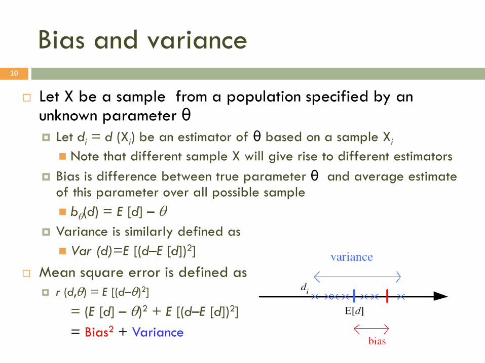
Let X be a sample from a population specified by an unknown parameter θ

Let di = d (Xi) be an estimator of θ based on a sample Xi

Note that different sample X will give rise to different estimators

Bias is difference between true parameter θ and average estimate of this parameter over all possible sample

b(d) = E [d] –

Variance is similarly defined as

Var (d)=E [(d–E [d])2]

Mean square error is defined as :

r (d,) = E [(d–)2]

= (E [d] – )2 + E [(d–E [d])2]

= Bias2 + Variance

Bayes’ Estimator 11

Sometimes before looking at a sample we (or experts) may have some prior information on the possible value range that a parameter θ may take

This information is quite useful and should be used especially when sample size is small

Prior information does not tell us “exactly” what the parameter value is

This uncertainty can be modeled by viewing θ as a random variable and defining a prior density p(θ)

Prior density tells us likely values of θ before looking at a sample

We combine this with what data tells us, i.e., likelihood density p(X|θ), use Bayes rule to get posterior density of θ

Example of translating domain specific prior information in to a prior probability density

Suppose a domain expert (from his years of experience) tells you that θ is approximately normal and with 90% confidence, θ lies between 5 and 9 symmetrically around 7

Then we can write p(θ) as a normal distribution with mean 7 and need to find its variance from the information provided

Statistics 101: If θ is normally distributed with mean μ and variance σ2, then (θ- μ)/σ is normally distributed with mean 0 and variance 1

From Normal distribution table P(-1.64<(θ-7)/ σ<1.64)=0.9 that is P(7-1.64σ<θ<7+1.64σ)=0.9

Setting 1.64σ=2, we see that θ can be modeled as Normally distributed random variable with mean 7 and variance (2/1.64)2

Bayes’ Estimator 12

Treat θ as a random var with prior p (θ)

Bayes’ rule: p (θ|X) = p(X|θ) p(θ) / p(X)

Full: p(x|X) = ∫ p(x|θ, X) p(θ|X) dθ =∫ p(x|θ) p(θ|X) dθ

If we are using prediction of the form y=g(x|θ) as in regression the then we can use the posterior density to predict that is y= ∫ g(x|θ) p(θ|X) dθ

Since computing this integration is often very difficult, we can use different options

Maximum a Posteriori (MAP): here we take the optimal value of the parameter θ as the one that maximizes posterior distribution

θMAP = argmaxθ p(θ|X)

We are using prior information here

Maximum Likelihood (ML): here we take the optimal value of the parameter θ as the one that maximizes data likelihood

θML = argmaxθ p(X|θ)

Prior information is not used here

Bayes’: use the expected or average value of parameter θ based on posterior distribution

θBayes’ = E[θ|X] = ∫ θ p(θ|X) dθ

Prior information is used here (but computing the expectation sometimes can be computationally expensive)

Bayes’ Estimator: Example

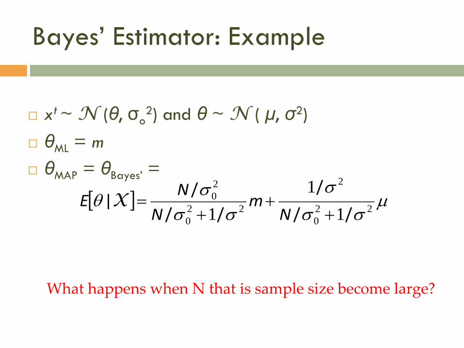
xt ~ N (θ, σo2) and θ ~ N ( μ, σ2)

θML = m

θMAP = θBayes’ =

22

0

2

22

0

2

0

1

1

1 //

/

//

/|

Nm

N

NE X

13

What happens when N that is sample size become large?

Parametric classification

Assume a car company is selling K different cars

Let us assume that the sole factor that a customer’s choice to buy a car is his or her yearly income

This is a K class classification problem, where number of input feature is one (annual salary) which is a continuous variable

P(Ci) is the prior probability of i-th type car that is proportion of customers who buy i-th type car

If the yearly income of such customers (who buys i-th type car) can be approximated (modeled) with a Gaussian then p(x|Ci), the probability that a customer who bought car type i has income x, can be taken to be N ( μi, σi

2)

We will say x ~ N ( μi, σi2)

where, μi is the mean income of such customers (who buys car type i) and σi

2 is income variance

14


Now we ca write the discriminant function for the i-th car type as

gi(x), where,

Note that this is essentially posterior probability P(Ci|x), we drop the denominator (the evidence P(x), as they are same for all class type

If we model class likelihood P(x|Ci) as a Gaussian as mentioned before then the discriminant function can be written as

Now, given a customer’s annual yearly income, we predict that he/she will buy i-th car type if gi(x)>gj(x), for all j≠ i

In other word, predicted class label is that car type whose discriminant function is the largest

15

iiiiii CPCxpxgCPCxpxg log| logor |

ii

iii

i

i

i

i

CPx

xg

xCxp

log log log

exp|

2

2

2

2

22

2

1

22

1


16

Given the sample

ML estimates of its parameters are (prior class probabilities and mean and variances of each Gaussians)

We compute discriminantfunction by plugging-in these parameter estimates into the discriminant function formula

,N

t

tt ,rx 1}{ X x

, i f

i f

ijx

xr

jt

it

ti C

C

0

1

t

ti

t

tii

t

i

t

ti

t

ti

t

it

ti

ir

rmx

sr

rx

mN

r

CP

2

2 ˆ

ii

iii CP

s

mxsxg ˆ log log log

2

2

22

2

1

How do we use? Example 1 17

Suppose bank is using a single variable, annual income, to classify a customer into low-risk or high-risk category

Annual income of each class (P(x|C) )is modeled as a Gaussian distribution

Using past data mean and variance of low risk customers were found to be $90K and $10K respectively

Using past data mean and variance of high risk customers were found to be $30K and $10K respectively

Prior class probabilities are same?

What is the decision rule for classification?



Ans: If annual income is greater than or equal to

$60K classify as low risk, otherwise high risk.

19

Equal variances

Single boundary at

halfway between means






Prior class probability for low risk customers is 1/4?





$60.18K classify as low risk, otherwise high

risk.






Prior class probability for low risk customers is 1/4?





$57.5K or less than or equal to -$237.5, classify

as low risk, otherwise high risk.






Prior class probabilities are same?





$46.8K or less than or equal to $23.2, classify as

low risk, otherwise high risk.

26

Variances are different

Two boundaries

Regression 28

In regression, we would like to write numeric output, called dependent variable, as a function of input, called the independent variable

We assume that numeric output is a sum of a deterministic function f of the input and a random noise, that is

Here f(x) is an unknown function that we would like to approximate by our estimator g(x| θ) defined up to a set of parameters θ

We assume that the error is zero mean Gaussian with variance σ2,

that is,

Then

Why? Statistics 101:

xfr

20~ ,N

2|~| ,N xgxrp

~)( n,scalar the a is and 0~ if 22 ,N,N yyxyx

Regression: From log-likelihood to error 29

We use maximum likelihood estimate (MLE) to estimate the parameters θ

Given a sample we write log-likelihood as

we can ignore the second term as it does not have any information related to θ

Plugging in the formula for Gaussian density, we get

Maximizing log-likelihood is same as minimizing empirical error (sum of squared error)

,N

t

tt ,rx 1}{ X

N

t

tN

t

tt

N

t

tt

xpxrp

rxp

11

1

log| log

, log|XL

2

12

2

2

1

|2

12log

2

|exp

2

1 log|

N

t

tt

ttN

t

xgrN

xgr

XL

2

1

|2

1|

N

t

tt xgrE X

Linear regression 31

In linear regression we model our estimator as

So, here, θ={w0,w1}

Taking derivative of the sum of the squared error with respect to w0 and w1 and setting them to zero we get

Which can be written in the matrix format where

therefore solution (estimate of parameters) is

0101 wxwwwxg tt ,|

t

t

t

tt

t

t

t

t

t

t

xwxwxr

xwNwr

2

10

10

yAw

t

t

tt

t

t

t

t

t

t

t

xr

r

w

w

xx

xN

yw 1

0

2A

yw1A

Polynomial regression 32

In the general case of polynomial regression, the model is a polynomial in x of order k

So, here, θ={w0,w1,w2,…,wk}

The model is still linear with respect to the parameters and taking the partial derivatives and setting them to zero, w get k+1 equations and k+1

Writing in matrix notation, our solution is

01

2

2012 wxwxwxwwwwwxg ttktkk

t ,,,,|

rwTT DDD

1

NNNN

k

k

r

r

r

xxx

xxx

xxx

2

1

22

2222

1211

1

1

1

r D

Estimating Bias and Variance 35

ti

t i

tti

t

tt

xgM

xg

xgxgNM

g

xfxgN

g

1

1

1

2

22

Variance

Bias

Suppose M samples Xi={xti , r

ti}, i=1,...,M

are used to fit gi (x), i =1,...,M

In real life we can not do this because we do not know what f is

Bias/Variance Dilemma 36

Example#1

Suppose, gi(x)=2

This is a constant fit function

has no variance because we do not use the data and all gi(x) are the same

But it has high bias, unless f(x) is close to 2

Example #2

Suppose gi(x)= ∑t rt

i/N

This has lower bias because we would expect the average in general to be closer to be a better estimate

However it will have higher variance because different sample Xi will have different average value

Typically, as we increase complexity of our model g

bias decreases (a better fit to data) and

variance increases (fit varies more with data)

This is known as Bias/Variance dilemma: (Geman et al., 1992)

37

bias

variance

f

gi g

f

Polynomial Regression 38

Best fit “min error”

39

Best fit, “elbow”

Model Selection 40

Cross-validation: Measure generalization accuracy by testing on data unused during training

Regularization: Penalize complex models

E’=error on data + λ model complexity

Akaike’s information criterion (AIC), Bayesian information criterion (BIC)

Minimum description length (MDL): Kolmogorov complexity, shortest description of data

Structural risk minimization (SRM)

Over-fitting vs Under-fitting 41

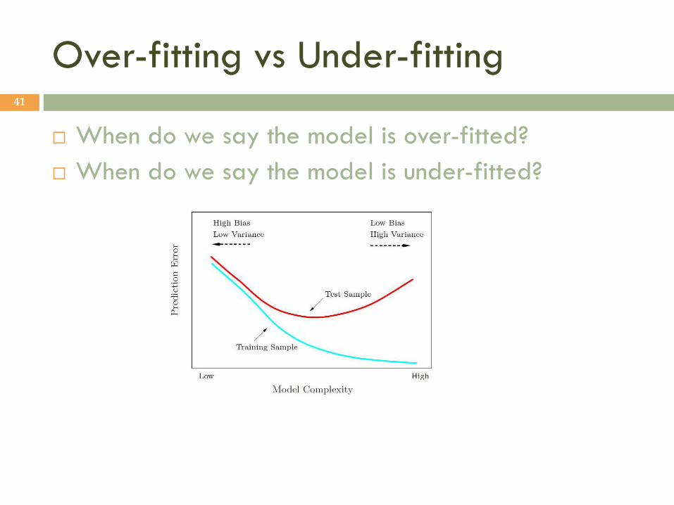
When do we say the model is over-fitted?

When do we say the model is under-fitted?

Over-fitting vs Under-fitting 42

The model is over-fitted when training error is very small but test error is large Too specific for the training sample, no generalization ability

The model is under-fitted when both training error and testing error are large The model is not complex enough to capture/represent functional

relationship f: x y

chapter 4: parametric methods - wichita state …sinha/teaching/fall17/cs697ab/slide/ch4.pdf ·...

Documents