chapter 4 neural network controller for harmonic elimination in multilevel...
TRANSCRIPT
62
CHAPTER 4
NEURAL NETWORK CONTROLLER FOR HARMONIC
ELIMINATION IN MULTILEVEL INVERTER
4.1 INTRODUCTION
Uninterruptible power supplies (UPSs) are emergency power
sources which have wide spread application in critical equipments, such as
computers, automated process controllers, and hospital instruments. With the
rapid growth in the use of high-efficiency power converters, more and more
electrical loads are nonlinear and generate harmonics. It is a big challenge for
a UPS to maintain a high-quality sinusoidal output voltage under a nonlinear
loading condition.
An NN is an interconnection of a number of artificial neurons that
simulates a biological brain system. It has the ability to approximate an
arbitrary function mapping and can achieve a higher degree of fault
tolerance. NNs have been successfully introduced into power electronics
circuits. For the harmonic elimination of PWM inverters, NN replaced a
large and memory-demanding look-up table to generate the switching angles
of a PWM inverter for a given modulation index (Xiao Sun et al 2002).
4.2 TRAINING METHODS
When an NN is used in system control, the NN can be trained
either on-line or off-line. In on-line training, since the weights and biases of
63
the NN are adaptively modified during the control process, it has better
adaptability to a nonlinear operating condition. The most popular training
algorithm for a feed forward NN is back propagation. It is attractive because
it is stable, robust, and efficient. However, the back propagation algorithm
involves a great deal of multiplication and derivation. If implemented in
software, it needs a very fast digital processor. If implemented in hardware, it
results in a rather complex circuitry.
Off-line training of an NN requires a large number of ex ample
patterns. These patterns may be obtained through simulations. Although the
weights and biases are fixed during the control process, the NN is a nonlinear
system that has much better robustness than a linear system. Moreover, the
forward calculation of the NN involves only addition, multiplication, and
sigmoidal-function wave shaping that can be implemented with simple and
low-cost analogue hardware. The fast-response and low-cost implementation
of the off-line trained NN are suitable for UPS inverter applications.
4.3 APPLICATIONS OF NEURAL NETWORKSIN
HARMONICS
The application of ANN is recently growing in power electronics
and drives area. A feed forward ANN basically implements nonlinear input-
output mapping. The computational delay of this mapping becomes large. The
optimal switching pattern Pulse Width modulation (PWM) strategies
constitute the best choice for high power, three-phase, voltage-controlled
inverters and for fixed frequency, fixed-voltage UPS systems. For any chosen
objective function, the optimal switching pattern depends on the desired
modulation index. In the existing practice, the switching patterns are
recomputed for all the required values of this index, and stored in look-up
tables of a microprocessor-based modulator. This requires a large memory
and computation of the switching angles in real time is, as yet, impossible. To
64
overcome this problem, attempts were made to use approximate formulas, at
the expense of reduced quality of the inverter voltage. Recently, alternate
methods of implementing these switching patterns have been developed.
Without using a real time solution of nonlinear harmonic elimination
equation, an ANN is trained off-line to output the switching angles for wanted
output voltage. The most disadvantage of this application is the use in training
stage the desired switching angles givenby the solving of the harmonic
elimination equation by the classical method, i.e., the Newton Raphson
method. This algorithm requires starting values for the angles and does not
always converge to the required solution. To give a solution to this problem,
powers electronics researches always study many novel control techniques to
reduce harmonics in such waveforms.
4.4 SELECTIVE HARMONIC ELIMINATION (SHE)STRATEGY
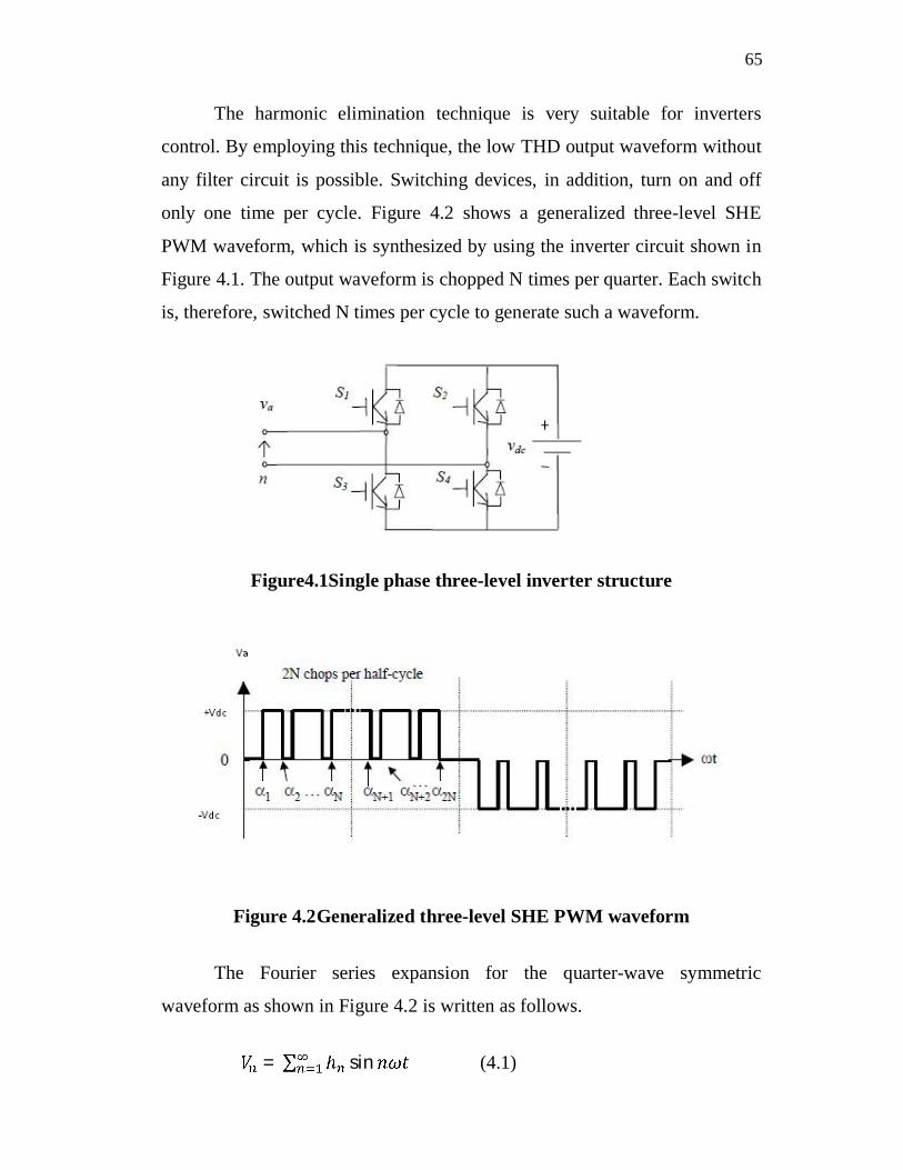
Single phase three level inverter structure is shown in Figure 4.1. It
has 4 switches. When switches S1 and S4 are turned on, the positive half cycle
of the output ac voltage is obtained. The negative half cycle of the ac voltages
are obtained by triggering switches S2 and S3. Various objective functions
can be used in the optimal control of an inverter. For the described study, the
classic harmonic elimination strategy was selected. It consists in determining
s optimal switching angles. The primary angles are limited to the first quarter
cycle of the inverter output line voltage (phase a) Figure4.1. Switching angles
in the remaining three quarters are referred to as secondary angles. The full-
cycle switching pattern must have the half-wave and quarter-wave symmetry
in order to eliminate even harmonics. Hence, the secondary angles are
linearly dependent on their primary counterparts Figure4.2. The resultant
optimal switching pattern yields a fundamental voltage corresponds to a given
value of the modulation index, whereas (s 1) low order, odd, and triple
harmonics are absent in the output voltage.
65
The harmonic elimination technique is very suitable for inverters
control. By employing this technique, the low THD output waveform without
any filter circuit is possible. Switching devices, in addition, turn on and off
only one time per cycle. Figure 4.2 shows a generalized three-level SHE
PWM waveform, which is synthesized by using the inverter circuit shown in
Figure 4.1. The output waveform is chopped N times per quarter. Each switch
is, therefore, switched N times per cycle to generate such a waveform.
Figure4.1Single phase three-level inverter structure
Figure 4.2Generalized three-level SHE PWM waveform
The Fourier series expansion for the quarter-wave symmetric
waveform as shown in Figure 4.2 is written as follows.
= sin (4.1)

66
= ( 1) cos (4.2)
Where, Nis the number of the switching angles per quarter.
k is the switching angles, which must satisfy the following condition
< (4.3)
Vdcis the amplitude of the dc source.
and n is the harmonic order.
From Equation (4.2), the nonlinear equations of SHE PWM
waveform can be written as follows.
cos cos ± cos = = (4.4)
cos 3 cos 3 ± cos 3 = (4.5)
.
.
.
cos cos ± cos = (4.6)
Where, =
In order control the fundamental amplitude and to eliminate the
lower order harmonics, the nonlinear transcendental equations must be solved
and the switching angles 1, 2, …, n are calculated offline to minimize the
harmonics for each modulation index in order to have a total output voltage
with a harmonic minimal distortion rate.

67
4.5 ARTIFICIAL NEURAL NETWORK
A typical multilayer ANN is shown in Figure.4.3. It consists of one
input layer, a middle layer and an output layer, where each layer has a
specific function. The input accepts an input data and distributes it to all
neurons in the middle layer. The input layer is usually passive and does not
alter the input data. The neurons in the middle layer act as feature detectors.
They encode in their weights a representation of the features present in the
input patterns. The output layer accepts a stimulus pattern from the middle
layer and passes a result to a transfer function block which usually applies a
nonlinear function and constructs the output response pattern of the network.
The number of hidden layers and the number of neurons in each hidden layer
depend on the network design consideration and there is no general rule for
an optimum number of hidden layers or nodes. The ANN to be used for the
generation of the optimal switching angles has a single input neuron fed by
the modulation index, one hidden layer and s outputs where each output
represents a switching angle.
Figure4.3 A typical multilayer ANN
1x1 1 1
2x2 2 2
nx3
K P
y1
y2
yp
y11
yk1
yk2
ykp
w1k
w12
w11
y12
y1py2p
y21y22
w21
w22
w2k
wn1wn2
wnk

68
The output of the neuron is given by the following equation
= ( + ) (4.7)
Where, y - the output of the neuron,
xi - the ith input to the neuron,
wi - the ith connection weight,
wo - the bias weight,
(.) - the transfer function of the neuron,
k - the number of connections with the neurons in the preceding
layer.
Figure4.4 Structure of a single neuron
Figure 4.4 shows the structure of a single neuron. The input signals
x1, x2, … , xk are normally continuous variables. Each of the input signals flows
through a gain or weight. The weights can be positive or negative
corresponding to acceleration or inhibition of the flow of signals. The
summing node accumulates all the input weighted signals and then passes to
69
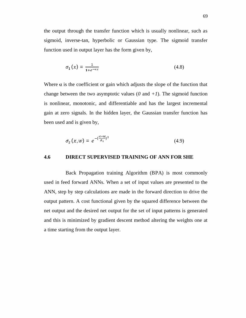
the output through the transfer function which is usually nonlinear, such as
sigmoid, inverse-tan, hyperbolic or Gaussian type. The sigmoid transfer
function used in output layer has the form given by,
( ) = (4.8)
Where is the coefficient or gain which adjusts the slope of the function that
change between the two asymptotic values (0 and +1). The sigmoid function
is nonlinear, monotonic, and differentiable and has the largest incremental
gain at zero signals. In the hidden layer, the Gaussian transfer function has
been used and is given by,
( , ) = ( ) (4.9)
4.6 DIRECT SUPERVISED TRAINING OF ANN FOR SHE
Back Propagation training Algorithm (BPA) is most commonly
used in feed forward ANNs. When a set of input values are presented to the
ANN, step by step calculations are made in the forward direction to drive the
output pattern. A cost functional given by the squared difference between the
net output and the desired net output for the set of input patterns is generated
and this is minimized by gradient descent method altering the weights one at
a time starting from the output layer.

70
Figure4.5 Direct Supervised Training of ANN for SHE
Figure4.6 ANN set for the Selective Harmonic Elimination
Figure 4.6 shows an ANN with a single input neuron fed by the
modulation index, l hidden neurons and s outputs each representing a
switching angle. The network was training using the Back Propagation
Algorithm (BPA). The training data extracted from the optimal switching
ANN
7 level
inverter
BPA
Selective
Harmonic
Elimination
Switching signal
generator
m1
2
s
1d
2d
ds
aSbScS
anVbnVcnV
1 1
1m
2 2
l S
2w
lw
1w
1lv
lsv
1
2
s

71
angles, designated by 1 to s as functions of the modulation index m.
Equation 4.10 gives the outputs of the ANN shown in Figure4.6.
= , , = 1, … , (4.10)
4.7 INDIRECT SUPERVISED TRAINING OF ANN FOR SHE
In this case, the neural network is trained to generate the switching
angles in a way to eliminate the first harmonics without the knowledge of the
desired switching angles given by the Newton Raphson method. The problem
which arises in this indirect learning paradigm is that the desired outputs of
the ANN, i.e. optimal angles, are unknown. To avoid this problem, we will
insert in series with the ANN the equivalent nonlinear system equations.
Therefore, instead of the minimization of the error between the switching
angles given by the ANN and the wished switching angles often unknown, we
will minimize the error at the output of the nonlinear system equation of the
harmonics to be eliminated. Figure 4.7 shows the diagram of the indirect
training strategy of artificial neuron networks used for harmonics elimination.
When the desired precision is obtained the output of the ANN is used to
generate the control sequence of the inverter.
Figure 4.7 Indirect Training of ANN for Selective Elimination Harmonic
ANN7-level
Inverter
BPA
( )H
Switchingsignal
generatorm
1
2
s
aSbScS
anVbnVcnV
/ 4
1dh
2 0dh0dsh
1h
sh

72
The ANN is trained by the back-propagation algorithm of the error
between the desired solutions of the nonlinear system equations to eliminate
the first harmonics and the output of this equation using the switching angle
given by the ANN.
4.8 BACK PROPAGATION NETWORK (BPN) FOR HARMONIC
ELIMINATION
The network to be utilized for the technique is depicted in
Figure 4.8. It consists of one input layer, one hidden layer and an output layer.
Switching angles are given as inputs and their harmonic voltages are taken as
outputs.
Figure 4.8 The network structure
The input layer, hidden layer and output layer of the network
consists of lN , hidN and 12HN neurons, respectively. To train the network,
Nhid
V3
21NN2 h
hidw
2N2 hidw
1N2 hidw
w222
w221 21N21 hw
w211
21Nh
hidN1w
w22w21
w12
1
2
w11
hidN2w
1
1
Input layer Hidden layer Output layer
2
1
2
w212 V1
hNV
Nl
2
lN
1N lw
2Nlw
hidlNNw
21N22 hw

73
an appropriate dataset needs to be generated from the dataset D and it is
shown in Figure 4.9.
)1()1()1( 1)1(1101
12)1(112012
11)1(111011
flff
l
l
NNNN
N
N
FNN
FN
FN
FN
FF
FN
FF
fHff
H
H
VVV
VVV
VVV
)1()1()1( 31
23212
13111
)2()2()2( 2)1(1202
22)1(122022
21)1(121021
flff
l
l
NNNN
N
N
FNN
FN
FN
FN
FF
FN
FF
fHff
H
H
VVV
VVV
VVV
)2()2()2( 31
23212
13111
()()( )1(10
2)1(2120
1)1(1110
INfIlIN
fIINfI
IlII
IlII
NNNNNNN
NNNN
NNNN
FNN
FN
FN
FN
FF
FN
FF
INfHIN
fIN
f
H
H
VVV
VVV
VVV
)()()( 31
23212
13111
Figure 4.9 The dataset trainD used to train the network
4.9 TRAINING ALGORITHM FOR HARMONIC ELIMINATION
The entire dataset is given as input to the neural network and
trained well using Back Propagation (BP) algorithm. The training process is
described below.
(i) Generate arbitrary weights in the interval maxmin,ww and assign it
to neurons of the hidden layer and the outer layer. Assign unity
weight to the neurons of the input layer.

74
(ii) Give the training dataset D as input to the network and determine
the BP error as follows
outT VVe (4.11)
In Equation (4.11), TV and outV are the target output and the
network outputs, respectively. From every output neuron of the
network, the elements of outV )( hV can be determined as follows
HidN
nnnhh ywV
1(4.12)
where,
l
jkl
N
j
jnn e
wy
1 1(4.13)
In Equation (4.12) hidN is the number of hidden neurons, nhw is the
assigned weight of the hn link of the network and hV is the
output of the thh output neuron. In Equation (4.13), ny is the output
of the thn hidden neuron.
(iii) On the basis of the obtained BP error, determine the change in
weights as follows
.V. ew out (4.14)
where, the learning rate , normally ranges from 0.2 to 0.5.
(iv) Determine new weights as follows,
www (4.15)

75
(v) Repeat the process from step (ii), until BP error gets reduced to a
least value, essentially, the condition to be satisfied is 0.1e .
Once the training process is completed, the network gets well-
prepared to evaluate any given unknown data.
4.10 SIMULATION RESULTS
The implementation of the Neural Network Control technique is
performed in the working platform of MATLAB (version 7.10). The
technique is implemented in such a way that it can eliminate the 3rd order and
5th order harmonics and so it can minimize the total harmonic distortion. The
output voltages of the Three H Bridges are given in Figure 4.10, 4.11 and
4.12.The output voltage performance of the inverter obtained for the
computed optimal switching angles are given in Figure 4.13. Output voltage
Vs time plot is given in Figure 4.14. FFT analysis of inverter output voltage is
shown in Figure 4.15.
Acomparison of the performance of Neural Network Controller and
Fuzzy Logic Controller with respect to the Total Harmonic Distortion
and the computational time with modulation index of 0.5 and sampling
frequency of 200KHzare listed in the Table 4.1. From the results
it is observed that Fuzzy logic controller gives better result than that of
neural network controller for the multilevel inverter considered for
simulation.

76
Figure 4.10 Output waveform of inverter bridge 1
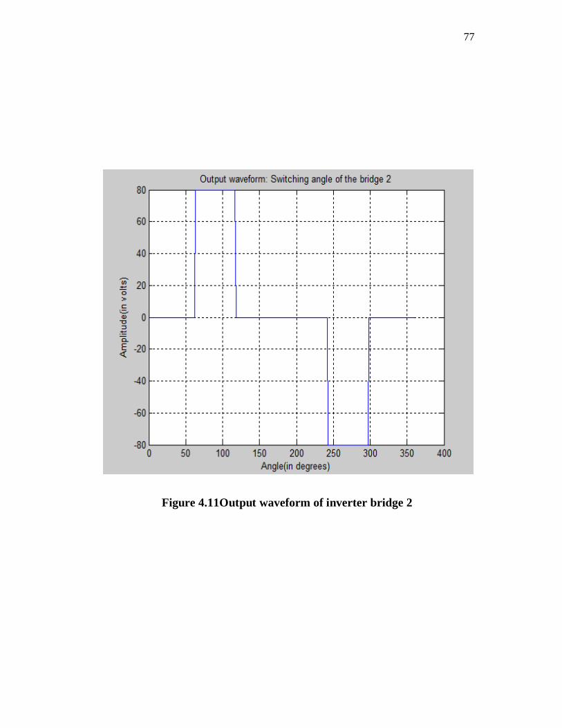
77
Figure 4.11Output waveform of inverter bridge 2
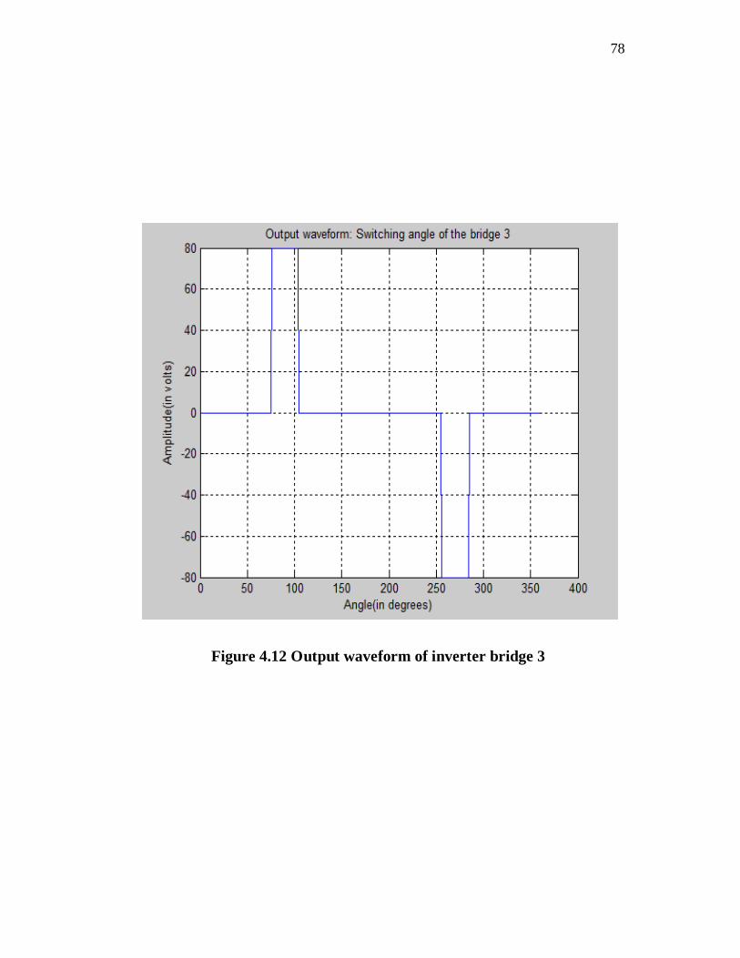
78
Figure 4.12 Output waveform of inverter bridge 3

79
Figure 4.13 Output waveform of the Inverter using neural network
controller

80
Figure 4.14 Output Voltage Vs Time plot of the Inverter usingneural
network controller
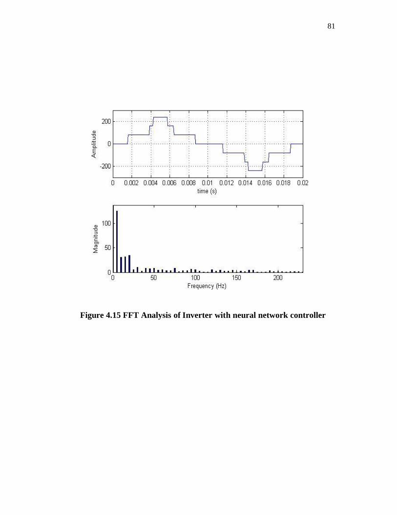
81
Figure 4.15 FFT Analysis of Inverter with neural network controller

82
Table 4.1 Comparative results of multilevel inverter with Neural
Network and Fuzzy Logic Controller
Methodologies Total harmonic
distortion (THD)
Computational
time in Seconds
Fuzzy Logic 1.8468 0.0795
Neural Network 4.2373 0.2021
BasilM.Saied et al (2008) found 3rd, 5th,7th, 9th and 11th harmonics
with the help of SHE-PWM technique on a single phase 3 level H bridge
inverter using Neural network and Fuzzy Logic. The 3rd and 5th harmonic
voltages for Neural Network controller were reported as 1% and 5%
respectively. Hence it is clear that the proposed Neural Network Controller
used in this thesis gives better result with the THD of 4.2%. Also it is
observed that Fuzzy Logic Controller is more accurate than Neural Network
Controller.
4.11 CONCLUSION
In this chapter, the use of the ANN to solve the selective harmonics
elimination problem in PWM inverters is proposed. This technique allows
successful voltage control of the fundamental as well as suppression of a
selective set of harmonics. The main advantage of the proposed method is
that it requires neither high computing power nor specialized ANN hardware.
The main drawback of this technique lies in the training phase, since, this
phase is quite complex and time consuming. The given simulation results
proving the feasibility of the proposed technique.