chapter 4 methodological choice and identification … · chapter 4: methodological choice and...
TRANSCRIPT
Chapter 4: Methodological Choice and Identification of Key Categories
2019 Refinement to the 2006 IPCC Guidelines for National Greenhouse Gas Inventories 4.1
CHAPTER 4
METHODOLOGICAL CHOICE AND IDENTIFICATION OF KEY CATEGORIES

Volume 1: General Guidance and Reporting
4.2 2019 Refinement to the 2006 IPCC Guidelines for National Greenhouse Gas Inventories
Authors Justin Goodwin (UK)
Newton Paciornik (Brazil), Michael Gillenwater (USA)
Contributing Author Timo Kareinen (Finland)
Chapter 4: Methodological Choice and Identification of Key Categories
2019 Refinement to the 2006 IPCC Guidelines for National Greenhouse Gas Inventories 4.3
Contents
4 Methodological Choice and Identification of Key Categories ...................................................................... 4.5
4.1 Introduction ............................................................................................................................................ 4.5
4.1.1 Definition ........................................................................................................................................ 4.5
4.1.2 Purpose of the key category analysis .............................................................................................. 4.5
4.1.3 General approach to identify key categories ................................................................................... 4.7
4.2 General rules for identification of key categories .................................................................................. 4.7
4.3 Methodological approaches to identify key categories ........................................................................ 4.16
4.3.1 Approach 1 to identify key categories ........................................................................................... 4.16
4.3.2 Approach 2 to identify key categories ........................................................................................... 4.20
4.3.3 Qualitative criteria to identify key categories ............................................................................... 4.20
4.4 Reporting and Documentation ............................................................................................................. 4.20
4.5 Examples of key category analysis ...................................................................................................... 4.21
References………………………………………………………………………………………………………4.32
Equations
Equation 4.1 (Updated) Level Assessment (Approach 1) .............................................................................. 4.16
Equation 4.2 (Updated) Trend Assessment (Approach 1) .............................................................................. 4.18
Figures
Figure 4.1 Decision Tree to choose a Good Practice method ...................................................... 4.6
Volume 1: General Guidance and Reporting
4.4 2019 Refinement to the 2006 IPCC Guidelines for National Greenhouse Gas Inventories
Tables
Table 4.1 (Updated) Suggested aggregation level of analysis for Approach 1 ............................................... 4.9
Table 4.2 (Updated) Spreadsheet for the Approach 1 analysis – Level Assessment ..................................... 4.17
Table 4.3 (Updated) Spreadsheet for the Approach 1 analysis – Trend Assessment .................................... 4.18
Table 4.4 (Updated) Summary of key category analysis ............................................................................... 4.21
Table 4.4a (New) Key categories ranks .................................................................................................... 4.21
Table 4.5 (Updated) Example of Approach 1 Level Assessment for Finland’s GHG Inventory for 2016 .... 4.22
Table 4.6 (Updated) Example of Approach 1 Trend Assessment for Finland's GHG inventory for 2016 .... 4.24
Table 4.9 (Updated) Example of Approach 2 Level Assessment for Finland’s GHG Inventory for 2016 .... 4.27
Table 4.10 (Updated) Example of Approach 2 Trend Assessment for Finland’s GHG Inventory for 2016 ... 4.28
Table 4.11 (Updated) Example of Summary of Key Category Analysis for Finland's GHG inventory for 2016 ........................................................................................................................ 4.30

Chapter 4: Methodological Choice and Identification of Key Categories
2019 Refinement to the 2006 IPCC Guidelines for National Greenhouse Gas Inventories 4.5
4 METHODOLOGICAL CHOICE AND IDENTIFICATION OF KEY CATEGORIES
Users are expected to go to Mapping Tables in Annex 1, before reading this chapter. This is required to correctly understand both the refinements made and how the elements in this chapter relate to the corresponding chapter in the 2006 IPCC Guidelines.
4.1 INTRODUCTION This chapter addresses how to decide on methods to apply and in using key category analysis1 to inform this choice. Methodological choice for individual source and sink categories is important in managing and where possible reducing the overall inventory uncertainty. Generally, inventory uncertainty is lower when emissions and removals are estimated using the most rigorous methods provided for each category or subcategory in the sectoral volumes of the 2006 IPCC Guidelines and its 2019 Refinement. However, these methods generally require more extensive resources for data collection, so it may not be feasible to use more rigorous method for every category of emissions and removals. It is therefore good practice to identify those categories that have the greatest contribution to overall inventory uncertainty in order to make the most efficient use of available resources. It is also important to identify categories that contribute significantly to the national totals to ensure that they are compiled accurately and that the data needed to update their estimates is sufficiently maintained. It is good practice for each country to identify its national key categories in a systematic and objective manner. By identifying these key categories in the national inventory, inventory compilers can prioritise their efforts and improve their overall estimates.
4.1.1 Definition Key categories are inventory categories which individually, or as a group of categories (for which a common method, emission factor and activity data are applied) are prioritised within the national inventory system because their estimates have a significant influence on a country’s total inventory of greenhouse gases in terms of the absolute level, the trend, or the level of uncertainty in emissions or removals. Whenever the term key category is used, it includes both source and sink categories.
4.1.2 Purpose of the key category analysis Within the National Inventory Arrangements (see Section 1.4a of Chapter 1, Volume 1), application of a key category analysis will help identifying the priority categories for which methods, activity data, emission factors and other parameters should be considered for regular update, more rigorously checked and reviewed and, where necessary or possible, improved as elaborated below:
• Regular update: Making sure the methods, data flows and country-specific emission factors are kept up to date and available for important regular estimate updates.
• More focussed checking and review: Making sure that specific quality assurance and quality control (QA/QC) activities are implemented for key categories. It is good practice to give additional attention to key categories with respect to QA/QC as described in Chapter 6, Quality Assurance/Quality Control and Verification, and in the sectoral volumes.
• Improvement: Improving accuracy of estimates and reducing overall uncertainty using higher tiered (more accurate) methods. In general, more detailed higher tier methods should be selected for key categories. Inventory compilers should use the category-specific methods presented in sectoral decision trees in Volumes 2-5. For most sources/sinks, higher tier (Tier 2 and 3) methods are suggested for key categories, although this is not always the case. For guidance on the specific application of this principle to key categories, it is good practice to refer to the decision trees and sector-specific guidance for the respective category and additional good practice guidance in chapters in sectoral volumes. In some cases, inventory compilers may be unable to adopt a higher tier method due to lack of resources. This may mean that they are unable to collect the required data for a higher tier or are unable to determine country specific emission factors and other data needed for Tier 2 and 3 methods. In these cases, although this is not accommodated in the category-specific decision trees, a Tier 1 approach can be used, and this possibility is identified in Figure 4.1. It should in these cases be clearly
1 In Good Practice Guidance for National Greenhouse Gas Inventories (GPG2000, IPCC, 2000), the concept was named ‘key
source categories’ and dealt with the inventory excluding the LULUCF Sector.

Volume 1: General Guidance and Reporting
4.6 2019 Refinement to the 2006 IPCC Guidelines for National Greenhouse Gas Inventories
documented why the methodological choice was not in line with the sectoral decision tree. Any key categories where the good practice method cannot be used should have priority for future improvements.
It is good practice for each country to identify and communicate its national key categories in a systematic and objective manner as presented in this chapter. Such a process will help countries to prioritise available resources for (key) category methods, data sources and assumptions and will lead to improved inventory quality, as well as greater confidence in the estimates that are developed.
Figure 4.1 Decision Tree to choose a Good Practice method
Start
Can databe collected without
significantly jeopardizing theresources for other key
categories?
Is thesource or sink category
considered as keycategory?
Are the dataavailable to follow
category-specific good practice guidance for the key
categories?
Make arrangements to collect data.
Estimate emissions orremovals following guidance for key categories presentedin the decision trees in the
sectoral Volumes 2-5.
Choose a method presentedin Volumes 2-5 appropriate toavailable data, and document
why category-specificguidance cannot be followed.
Choose a method presentedin Volumes 2-5 appropriate
to available data.
Yes
Yes
Yes
No
No
Box 1
Box 2
Box 3
No
Chapter 4: Methodological Choice and Identification of Key Categories
2019 Refinement to the 2006 IPCC Guidelines for National Greenhouse Gas Inventories 4.7
4.1.3 General approach to identify key categories Key category analysis should be applied in all circumstances of inventory compilation no matter how simple or basic the inventory is. A category can be identified as a key for different reasons. These include:
• Level: Their absolute level of emissions/removals for a particular year of interest.
• Trend: Their change across a time series. Particularly important for categories that are showing increasing or decreasing emissions or removal trends across a time series.
• Uncertainty: If a category’s contribution to the GHG inventory total or trend uncertainty is high for relevant years or year spans, then the category should be identified as key.
• In addition to making a quantitative determination of key categories, it is good practice to consider the qualitative criteria for identifying categories that are likely to need prioritised attention (e.g. expected significant trends, categories not estimated or with suspected high uncertainty) as described in more detail in Section 4.3.3.
Section 4.3 presents the detailed methodology for the above cases of key category analysis under two approaches. Approach 1 where key category analysis is done without incorporating uncertainties and approach 2 where information on uncertainties is included.
As explained in Section 4.1.2 above, the main objective of key category analysis is to identify and prioritise key categories within the inventory management system. Therefore, it is helpful to consolidate the different analysis of the level and trend into a single summary list of key categories. This makes engagement with key stakeholders easier and communication of the key categories priorities possible.
Guidance on reporting and documentation of the key category analysis is provided in Section 4.4. Section 4.5 gives examples for key category identification.
4.2 GENERAL RULES FOR IDENTIFICATION OF KEY CATEGORIES
The following guidance describes good practice in determining the appropriate level of disaggregation of GHG estimates to identify key categories, additional to those presented in the 2006 IPCC Guidelines. The results of the key category analysis will be most useful for prioritising data gathering and estimation activities if the analysis is done at a level of aggregation aligned with countries' use of methods, data sources and assumptions. Disaggregation to very low levels of subcategories that are all covered by a single method and use of emission factor should be avoided since it will split an important aggregated category into many small subcategories that may be no longer considered as key. Countries should establish their own aggregations or disaggregation of categories accordingly and considering the guidance provided below. Countries using Approach 2 will need to align the level of aggregation with that used for the uncertainty analysis. This will be facilitated by an approach which is aggregated/disaggregated based on methodology and in particular uncertainties. The following principles can be followed in designing the analysis and in choosing the level of aggregation or disaggregation for key categories:
• IPCC categories: All relevant sectors and categories that contribute to the GHG inventory totals should be included in the key category analysis. Countries should also consider the relative importance of memo items such as international transportation and biomass burning to ensure that the calculations for these items are adequately addressed when designing improvement activities. The analysis should be performed at the level of categories or subcategories at which the IPCC methods are applied in the inventory. Over time, as estimates are updated/refined and higher tier approaches applied to categories and/or subcategories, the aggregations for key category analysis may change. Countries can consider the disaggregation of categories and subcategories by fuel or other relevant activity differentiators (e.g. livestock/management types etc.) where activity data, assumptions and/or emission factors are from different sources and/or uncertainties are likely to be significantly different. For Approach 2, possible cross-correlations between categories and/or subcategories should be taken into account when considering category aggregation 2 . When using Approach 2, the assumptions about such correlations should be the same when assessing uncertainties and identifying key categories (see Chapter 3, Uncertainties).
2 In practice, the effect of correlations for key category analysis should be taken into account in the disaggregation level used
for the Approach 2 assessment (for more advice on correlations in uncertainty analysis, see Chapter 3).
Volume 1: General Guidance and Reporting
4.8 2019 Refinement to the 2006 IPCC Guidelines for National Greenhouse Gas Inventories
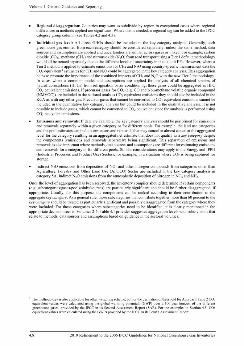
• Regional disaggregation: Countries may want to subdivide by region in exceptional cases where regional differences in methods applied are significant. Where this is needed, a regional tag can be added to the IPCC category group column (see Tables 4.2 and 4.3).
• Individual gas level: All direct GHGs should be included in the key category analysis. Generally, each greenhouse gas emitted from each category should be considered separately, unless the same method, data sources and assumptions are applied and uncertainties are similar across gases or linked. For example, carbon dioxide (CO2), methane (CH4) and nitrous oxide (N2O) from road transport using a Tier 1 default methodology would all be treated separately due to the different levels of uncertainty in the default EFs. However, where a Tier 2 method is applied to estimate emissions for CH4 and N2O using country-specific measurement data the CO2 equivalent3 estimates for CH4 and N2O could be aggregated in the key category analysis. This aggregation helps to promote the importance of the combined impacts of CH4 and N2O with the new Tier 2 methodology. In cases where a common model and assumptions are applied for analysis of all chemical species of hydrofluorocarbons (HFCs) from refrigeration or air conditioning, these gases could be aggregated as HFC CO2 equivalent emissions. If precursor gases for CO2 (e.g. CO and Non-methane volatile organic compound (NMVOC)) are included in the national totals as CO2 equivalent emissions they should also be included in the KCA as with any other gas. Precursor gases that cannot be converted to CO2 equivalent emissions cannot be included in the quantitative key category analysis but could be included in the qualitative analysis. It is not possible to include gases, which cannot be converted to CO2 equivalent since the analysis is performed using CO2 equivalent emissions.
• Emissions and removals: If data are available, the key category analysis should be performed for emissions and removals separately within a given category or for different pools. For example, the land use categories and the pool estimates can include emissions and removals that may cancel or almost cancel at the aggregated level for the category resulting in an aggregated net estimate that does not qualify as a key category despite the components (emissions and removals separately) being significant. This separation of emissions and removals is also important where methods, data sources and assumptions are different for estimating emissions and removals for a category or for different pools. Similar considerations may apply in the Energy and IPPU (Industrial Processes and Product Use) Sectors, for example, in a situation where CO2 is being captured for storage.
• Indirect N2O emissions from deposition of NOx and other nitrogen compounds from categories other than Agriculture, Forestry and Other Land Use (AFOLU) Sector are included in the key category analysis in category 5A, Indirect N2O emissions from the atmospheric deposition of nitrogen in NOx and NH3.
Once the level of aggregation has been resolved, the inventory compiler should determine if certain components (e.g. subcategories/gases/pools/sinks/sources) are particularly significant and should be further disaggregated, if appropriate. Usually, for this purpose, the components can be ranked according to their contribution to the aggregate key category. As a general rule, those subcategories that contribute together more than 60 percent to the key category should be treated as particularly significant and possibly disaggregated from the category where they were included. For those categories where subcategories need to be identified, it is clearly mentioned in the appropriate decision trees in Volumes 2-5. Table 4.1 provides suggested aggregation levels with subdivisions that relate to methods, data sources and assumptions based on guidance in the sectoral volumes.
3 The methodology is also applicable for other weighting scheme, but for the derivation of threshold for Approach 1 and 2 CO2
equivalent values were calculated using the global warming potentials (GWP) over a 100-year horizon of the different greenhouse gases, provided by the IPCC in its Second Assessment Report (SAR). For the examples in Section 4.5, CO2 equivalent values were calculated using the GWPs provided by the IPCC in its Fourth Assessment Report.

Chapter 4: Methodological Choice and Identification of Key Categories
2019 Refinement to the 2006 IPCC Guidelines for National Greenhouse Gas Inventories 4.9
4 Only disaggregate further by subcategory, fuel and/or gas where activity data and emission factors are from different sources
and/or uncertainties are significantly different.
TABLE 4.1 (UPDATED) SUGGESTED AGGREGATION LEVEL OF ANALYSIS FOR APPROACH 1A
Source and Sink Categories to be assessed in Key Category Analysis Gases to be
assessed separately c
Category aggregation/disaggregation considerations4
Category Codes b Category Names b
Energy
1A1 & 1A2
Energy and Manufacturing Industry Fuel Combustion Activities CO2, CH4, N2O
These categories should be disaggregated according to methods, data sources, assumptions applied and known or likely differences in uncertainty. Estimates compiled from a common set of activity data and emission factors (e.g. energy balances and default or average country specific emission factors) with similar uncertainties can be aggregated. Common reasons for disaggregation can include differences in uncertainty for estimates of emissions for different fuels (disaggregation by main fuel type) or the application of Tier 2 or 3 methods for categories or sub-categories.
1A3a Fuel Combustion Activities - Transport - Civil Aviation CO2, CH4, N2O
Disaggregation could be considered where data for different fuels is sourced from different data providers and different methods are used for small and major airports.
1A3b Fuel Combustion Activities - Transport - Road transportation
CO2, CH4, N2O Disaggregate by fuel if fuel data is sourced from different data providers and likely to have different levels of accuracy.
1A3c Fuel Combustion Activities - Transport - Railways
CO2, CH4, N2O Disaggregation could be considered where data (e.g. on fuels) is sourced from different data providers and different methods are used for different types of transport.
1A3d Fuel Combustion Activities - Transport - Water-borne Navigation
CO2, CH4, N2O Disaggregation could be considered where data (e.g. on fuels) is sourced from different data providers and different methods are used for different types of transport.
1A3e Fuel Combustion Activities - Transport - Other Transportation
CO2, CH4, N2O Disaggregation could be considered where data (e.g. on fuels) is sourced from different data providers and different methods are used for different types of transport.
1A4 Fuel Combustion Activities - Other Sectors
CO2, CH4, N2O
1A5 Fuel Combustion Activities - Non-Specified
CO2, CH4, N2O
Volume 1: General Guidance and Reporting
4.10 2019 Refinement to the 2006 IPCC Guidelines for National Greenhouse Gas Inventories
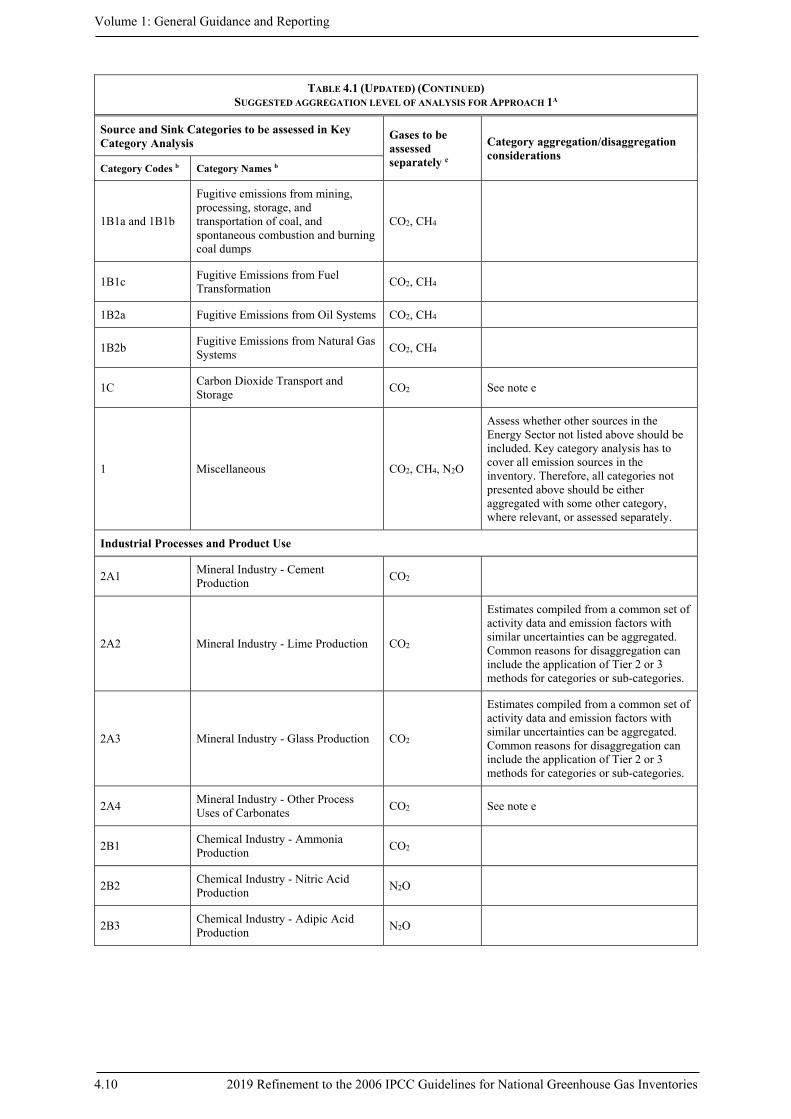
TABLE 4.1 (UPDATED) (CONTINUED) SUGGESTED AGGREGATION LEVEL OF ANALYSIS FOR APPROACH 1A
Source and Sink Categories to be assessed in Key Category Analysis
Gases to be assessed separately c
Category aggregation/disaggregation considerations
Category Codes b Category Names b
1B1a and 1B1b
Fugitive emissions from mining, processing, storage, and transportation of coal, and spontaneous combustion and burning coal dumps
CO2, CH4
1B1c Fugitive Emissions from Fuel Transformation CO2, CH4
1B2a Fugitive Emissions from Oil Systems CO2, CH4
1B2b Fugitive Emissions from Natural Gas Systems CO2, CH4
1C Carbon Dioxide Transport and Storage CO2 See note e
1 Miscellaneous CO2, CH4, N2O
Assess whether other sources in the Energy Sector not listed above should be included. Key category analysis has to cover all emission sources in the inventory. Therefore, all categories not presented above should be either aggregated with some other category, where relevant, or assessed separately.
Industrial Processes and Product Use
2A1 Mineral Industry - Cement Production CO2
2A2 Mineral Industry - Lime Production CO2
Estimates compiled from a common set of activity data and emission factors with similar uncertainties can be aggregated. Common reasons for disaggregation can include the application of Tier 2 or 3 methods for categories or sub-categories.
2A3 Mineral Industry - Glass Production CO2
Estimates compiled from a common set of activity data and emission factors with similar uncertainties can be aggregated. Common reasons for disaggregation can include the application of Tier 2 or 3 methods for categories or sub-categories.
2A4 Mineral Industry - Other Process Uses of Carbonates CO2 See note e
2B1 Chemical Industry - Ammonia Production CO2
2B2 Chemical Industry - Nitric Acid Production N2O
2B3 Chemical Industry - Adipic Acid Production N2O
Chapter 4: Methodological Choice and Identification of Key Categories
2019 Refinement to the 2006 IPCC Guidelines for National Greenhouse Gas Inventories 4.11
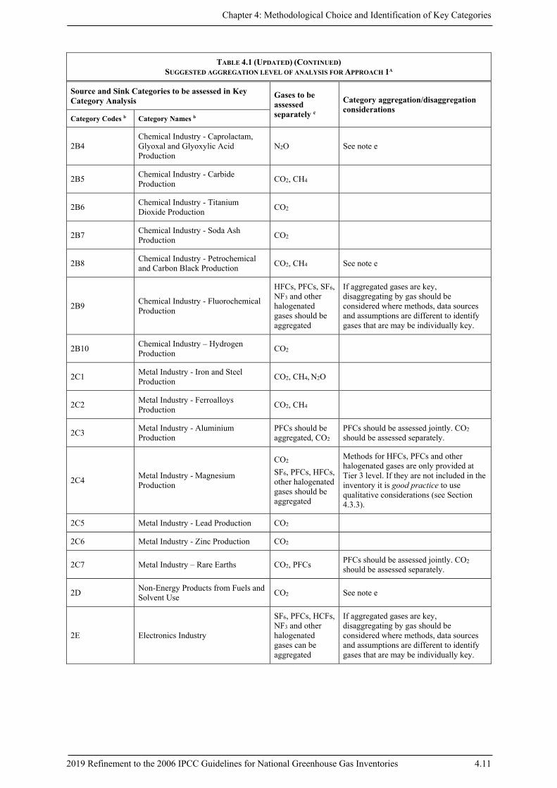
TABLE 4.1 (UPDATED) (CONTINUED) SUGGESTED AGGREGATION LEVEL OF ANALYSIS FOR APPROACH 1A
Source and Sink Categories to be assessed in Key Category Analysis
Gases to be assessed separately c
Category aggregation/disaggregation considerations
Category Codes b Category Names b
2B4 Chemical Industry - Caprolactam, Glyoxal and Glyoxylic Acid Production
N2O See note e
2B5 Chemical Industry - Carbide Production CO2, CH4
2B6 Chemical Industry - Titanium Dioxide Production CO2
2B7 Chemical Industry - Soda Ash Production CO2
2B8 Chemical Industry - Petrochemical and Carbon Black Production CO2, CH4 See note e
2B9 Chemical Industry - Fluorochemical Production
HFCs, PFCs, SF6, NF3 and other halogenated gases should be aggregated
If aggregated gases are key, disaggregating by gas should be considered where methods, data sources and assumptions are different to identify gases that are may be individually key.
2B10 Chemical Industry – Hydrogen Production CO2
2C1 Metal Industry - Iron and Steel Production CO2, CH4, N2O
2C2 Metal Industry - Ferroalloys Production CO2, CH4
2C3 Metal Industry - Aluminium Production
PFCs should be aggregated, CO2
PFCs should be assessed jointly. CO2 should be assessed separately.
2C4 Metal Industry - Magnesium Production
CO2 SF6, PFCs, HFCs, other halogenated gases should be aggregated
Methods for HFCs, PFCs and other halogenated gases are only provided at Tier 3 level. If they are not included in the inventory it is good practice to use qualitative considerations (see Section 4.3.3).
2C5 Metal Industry - Lead Production CO2
2C6 Metal Industry - Zinc Production CO2
2C7 Metal Industry – Rare Earths CO2, PFCs PFCs should be assessed jointly. CO2 should be assessed separately.
2D Non-Energy Products from Fuels and Solvent Use CO2 See note e
2E Electronics Industry
SF6, PFCs, HCFs, NF3 and other halogenated gases can be aggregated
If aggregated gases are key, disaggregating by gas should be considered where methods, data sources and assumptions are different to identify gases that are may be individually key.

Volume 1: General Guidance and Reporting
4.12 2019 Refinement to the 2006 IPCC Guidelines for National Greenhouse Gas Inventories
TABLE 4.1 (UPDATED) (CONTINUED) SUGGESTED AGGREGATION LEVEL OF ANALYSIS FOR APPROACH 1A
Source and Sink Categories to be assessed in Key Category Analysis
Gases to be assessed separately c
Category aggregation/disaggregation considerations
Category Names b Category Names b
2F1 Product Uses as Substitutes for Ozone Depleting Substances - Refrigeration and Air Conditioning
HFCs and PFCs can be aggregated See note e
2F2 Product Uses as Substitutes for Ozone Depleting Substances - Foam Blowing Agents
HFCs can be aggregated
2F3 Product Uses as Substitutes for Ozone Depleting Substances - Fire Protection
HFCs, PFCs can be aggregated
2F4 Product Uses as Substitutes for Ozone Depleting Substances - Aerosols
HFCs, PFCs can be aggregated
2F5 Product Uses as Substitutes for Ozone Depleting Substances - Solvents
HFCs, PFCs can be aggregated
2F6 Product Uses as Substitutes for Ozone Depleting Substances - Other Applications
HFCs, PFCs can be aggregated
2G Other Product Manufacture and Use
SF6 and PFCs can be aggregated. N2O treated separately
If aggregated gases are key, disaggregating by gas should be considered where methods, data sources and assumptions are different to identify gases that are may be individually key. N2O should be assessed separately.
2 Miscellaneous
CO2, CH4, N2O should be assessed separately. HFCs, PFCs and SF6, other halogenated gases can be aggregated
Assess whether other sources in the IPPU Sector not listed above should be included. Key category analysis should cover all emission sources in the inventory. Therefore, all categories not presented above should be either aggregated with some other category, where relevant, or assessed separately.
Agriculture, Forestry and Other Land Use
3A1 Livestock: Enteric Fermentation CH4
If there are differences in the data sources, assumptions applied and uncertainties for the different animal types and or management/feed practices or if a sub-category accounts for more than 25 percent of the emissions of the category then these should also be disaggregated.
3A2 Livestock: Manure Management CH4, N2O
If there are also differences in the data sources, assumptions applied and uncertainties for the different animal types and or management practices or if a sub-category accounts for more than 25 percent of the emissions of the category then these should also be disaggregated.
Chapter 4: Methodological Choice and Identification of Key Categories
2019 Refinement to the 2006 IPCC Guidelines for National Greenhouse Gas Inventories 4.13
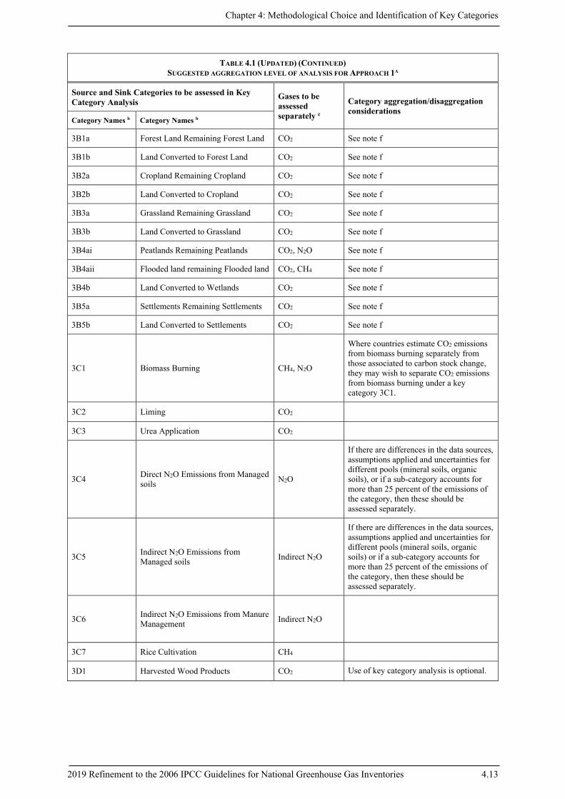
TABLE 4.1 (UPDATED) (CONTINUED) SUGGESTED AGGREGATION LEVEL OF ANALYSIS FOR APPROACH 1A
Source and Sink Categories to be assessed in Key Category Analysis
Gases to be assessed separately c
Category aggregation/disaggregation considerations
Category Names b Category Names b
3B1a Forest Land Remaining Forest Land CO2 See note f
3B1b Land Converted to Forest Land CO2 See note f
3B2a Cropland Remaining Cropland CO2 See note f
3B2b Land Converted to Cropland CO2 See note f
3B3a Grassland Remaining Grassland CO2 See note f
3B3b Land Converted to Grassland CO2 See note f
3B4ai Peatlands Remaining Peatlands CO2, N2O See note f
3B4aii Flooded land remaining Flooded land CO2, CH4 See note f
3B4b Land Converted to Wetlands CO2 See note f
3B5a Settlements Remaining Settlements CO2 See note f
3B5b Land Converted to Settlements CO2 See note f
3C1 Biomass Burning CH4, N2O
Where countries estimate CO2 emissions from biomass burning separately from those associated to carbon stock change, they may wish to separate CO2 emissions from biomass burning under a key category 3C1.
3C2 Liming CO2
3C3 Urea Application CO2
3C4 Direct N2O Emissions from Managed soils N2O
If there are differences in the data sources, assumptions applied and uncertainties for different pools (mineral soils, organic soils), or if a sub-category accounts for more than 25 percent of the emissions of the category, then these should be assessed separately.
3C5 Indirect N2O Emissions from Managed soils Indirect N2O
If there are differences in the data sources, assumptions applied and uncertainties for different pools (mineral soils, organic soils) or if a sub-category accounts for more than 25 percent of the emissions of the category, then these should be assessed separately.
3C6 Indirect N2O Emissions from Manure Management Indirect N2O
3C7 Rice Cultivation CH4
3D1 Harvested Wood Products CO2 Use of key category analysis is optional.

Volume 1: General Guidance and Reporting
4.14 2019 Refinement to the 2006 IPCC Guidelines for National Greenhouse Gas Inventories
TABLE 4.1 (UPDATED) (CONTINUED) SUGGESTED AGGREGATION LEVEL OF ANALYSIS FOR APPROACH 1A
Source and Sink Categories to be assessed in Key Category Analysis
Gases to be assessed separately c
Category aggregation/disaggregation considerations
Category Names b Category Names b
3
Miscellaneous e.g. non-CO2 emissions from biomass burning in forestland, cropland, grassland and wetlands, CH4 and N2O from the burning of drained organic soils, the CH4 and N2O from rewetting of organic soils and N2O from aquaculture
CO2, CH4, N2O
Assess whether other sources or sinks in the AFOLU Sector not listed above should be aggregated or included separately. Key category analysis has to cover all emission sources and sinks in the inventory. Therefore, all categories not presented above should be either aggregated with some other category, where relevant, or assessed separately.
Waste
4A Solid Waste Disposal CH4
This category should be disaggregated according to methods, data sources, assumptions applied and known or likely differences in uncertainty. Estimates compiled from a common set of activity data and emission factors with similar uncertainties can be aggregated. E.g. if there are significant differences in methodology and uncertainty for different types of solid waste disposal (managed and unmanaged sites) these should be disaggregated.
4B Biological Treatment of Solid Waste CH4, N2O
4C Incineration and Open Burning of Waste CO2, CH4, N2O
4D Wastewater Treatment and Discharge CH4, N2O
If there are differences in data sources, assumptions applied and uncertainties for different types of wastewater treatment (domestic or industrial wastewater and or different discharge routes) these should be disaggregated. Estimates compiled from a common set of activity data and emission factors with similar uncertainties can be aggregated.
4 Miscellaneous CO2, CH4, N2O
Assess whether other sources in the Waste Sector not listed above should be included. Key category analysis has to cover all emission sources in the inventory. Therefore, all categories not presented above should be either aggregated with some other category, where relevant, or assessed separately.
5A Indirect N2O Emissions from the atmospheric deposition of nitrogen in NOx and NH3
Indirect N2O
5B Other CO2, CH4, N2O, SF6, PFCs, HFCs
Include sources and sinks reported under 5B. Key category assessment has to cover all emission sources in the inventory. Therefore, all categories not presented above should be either aggregated with some other category, where relevant, or assessed separately.
Chapter 4: Methodological Choice and Identification of Key Categories
2019 Refinement to the 2006 IPCC Guidelines for National Greenhouse Gas Inventories 4.15
TABLE 4.1 (UPDATED) (CONTINUED) SUGGESTED AGGREGATION LEVEL OF ANALYSIS FOR APPROACH 1A
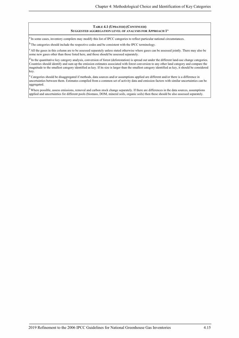
a In some cases, inventory compilers may modify this list of IPCC categories to reflect particular national circumstances. b The categories should include the respective codes and be consistent with the IPCC terminology. c All the gases in this column are to be assessed separately unless stated otherwise where gases can be assessed jointly. There may also be some new gases other than those listed here, and those should be assessed separately. d In the quantitative key category analysis, conversion of forest (deforestation) is spread out under the different land-use change categories. Countries should identify and sum up the emission estimates associated with forest conversion to any other land category and compare the magnitude to the smallest category identified as key. If its size is larger than the smallest category identified as key, it should be considered key. e Categories should be disaggregated if methods, data sources and/or assumptions applied are different and/or there is a difference in uncertainties between them. Estimates compiled from a common set of activity data and emission factors with similar uncertainties can be aggregated. f Where possible, assess emissions, removal and carbon stock change separately. If there are differences in the data sources, assumptions applied and uncertainties for different pools (biomass, DOM, mineral soils, organic soils) then these should be also assessed separately.
Volume 1: General Guidance and Reporting
4.16 2019 Refinement to the 2006 IPCC Guidelines for National Greenhouse Gas Inventories
4.3 METHODOLOGICAL APPROACHES TO IDENTIFY KEY CATEGORIES
No refinement.
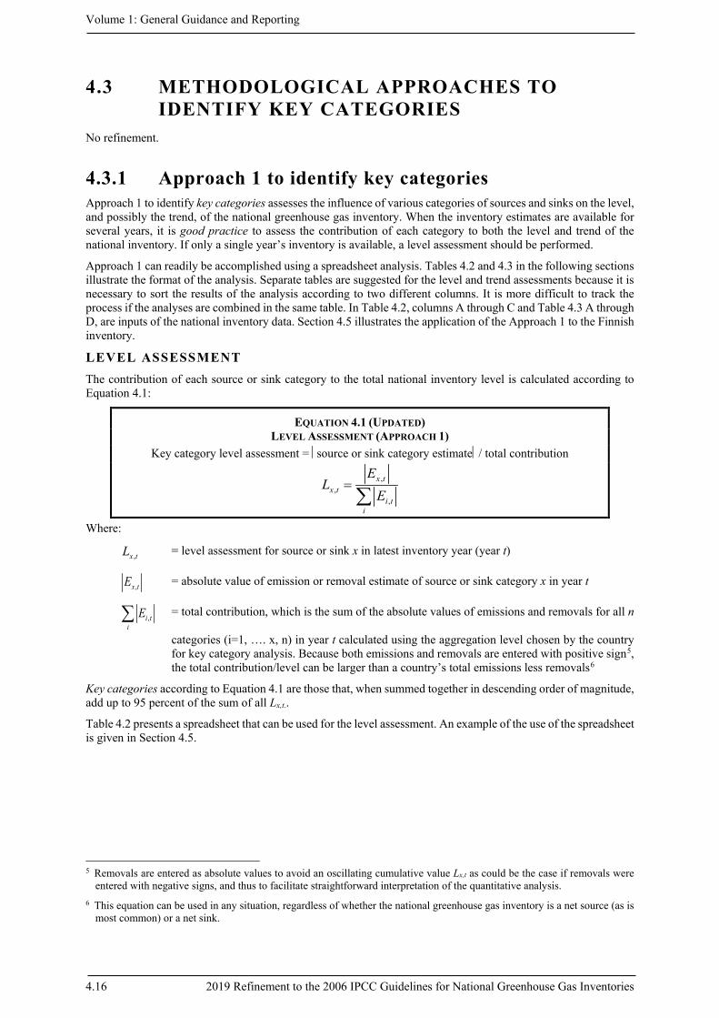
4.3.1 Approach 1 to identify key categories Approach 1 to identify key categories assesses the influence of various categories of sources and sinks on the level, and possibly the trend, of the national greenhouse gas inventory. When the inventory estimates are available for several years, it is good practice to assess the contribution of each category to both the level and trend of the national inventory. If only a single year’s inventory is available, a level assessment should be performed.
Approach 1 can readily be accomplished using a spreadsheet analysis. Tables 4.2 and 4.3 in the following sections illustrate the format of the analysis. Separate tables are suggested for the level and trend assessments because it is necessary to sort the results of the analysis according to two different columns. It is more difficult to track the process if the analyses are combined in the same table. In Table 4.2, columns A through C and Table 4.3 A through D, are inputs of the national inventory data. Section 4.5 illustrates the application of the Approach 1 to the Finnish inventory.
LEVEL ASSESSMENT The contribution of each source or sink category to the total national inventory level is calculated according to Equation 4.1:
EQUATION 4.1 (UPDATED) LEVEL ASSESSMENT (APPROACH 1)
Key category level assessment = source or sink category estimate/ total contribution
,,
,
x tx t
i ti
EL
E=∑
Where:
,x tL = level assessment for source or sink x in latest inventory year (year t)
,x tE = absolute value of emission or removal estimate of source or sink category x in year t
,i ti
E∑ = total contribution, which is the sum of the absolute values of emissions and removals for all n
categories (i=1, …. x, n) in year t calculated using the aggregation level chosen by the country for key category analysis. Because both emissions and removals are entered with positive sign5, the total contribution/level can be larger than a country’s total emissions less removals6
Key categories according to Equation 4.1 are those that, when summed together in descending order of magnitude, add up to 95 percent of the sum of all Lx,t..
Table 4.2 presents a spreadsheet that can be used for the level assessment. An example of the use of the spreadsheet is given in Section 4.5.
5 Removals are entered as absolute values to avoid an oscillating cumulative value Lx,t as could be the case if removals were
entered with negative signs, and thus to facilitate straightforward interpretation of the quantitative analysis. 6 This equation can be used in any situation, regardless of whether the national greenhouse gas inventory is a net source (as is
most common) or a net sink.

Chapter 4: Methodological Choice and Identification of Key Categories
2019 Refinement to the 2006 IPCC Guidelines for National Greenhouse Gas Inventories 4.17
TABLE 4.2 (UPDATED) SPREADSHEET FOR THE APPROACH 1 ANALYSIS – LEVEL ASSESSMENT
A B C D E F G
Category Codes and
Names
Greenhouse Gas
Latest Year Estimate
[in CO2 eq. units]
,x tE
Absolute Value of
Latest Year Estimate
,x tE
Level Assessment
,x tL
Cumulative Total of
Column E
Rank of Absolute Value of
Latest Year Estimate
Column D
Total ,i ti
E∑ 1
Where:
Column A: = description of category (see Section 4.2 above)
Column B: = greenhouse gas from the category
Column C: = value of emission or removal estimate of category 𝑥𝑥 in latest inventory year (year t) in CO2 equivalent units
Column D: = absolute value of emission or removal estimate of category x in year t
Column E: = level assessment following Equation 4.1
Column F: = cumulative total of Column E
Column G: = rank of absolute value of latest year estimate Column D
Inputs to Columns A-C will be available from the inventory. The total of Column C presents the net emissions and removals unless emissions and removals are presented separately. In Column D, absolute values are taken from each value in Column C. The sum of all entries in Column D is entered in the total line of Column D (note that this total may not be the same as the total net emissions and removals). In Column E, the level assessment is computed according to Equation 4.1. Once the entries in Column E are computed, the categories in the table should be sorted in descending order of magnitude according to Column E. After this step, the cumulative total summed in Column E can be calculated into Column F. Key categories are those that, when summed together in descending order of magnitude, add up to 95 percent of the total in Column F. Where the method is applied correctly, the sum of entries in Column E must be 1. The rationale for the choice of the 95 percent threshold for the Approach 1 builds on Rypdal and Flugsrud (2001) and is presented in GPG2000, Section 7.2.1.1 in Chapter 7.
It is also good practice to examine categories identified between threshold of 95 percent and 97 percent carefully with respect to the qualitative criteria (see Section 4.3.3).
The level assessment should be performed for the base year of the inventory and for the latest inventory year (year t). If estimates for the base year have changed or been recalculated, the base year analysis should be updated. Key category analysis can also be updated for other recalculated years. In many cases, however, it is sufficient to derive conclusions regarding methodological choice, resource prioritisation or QA/QC procedures without an updated key category analysis for the entire inventory time series. Any category that meets the threshold for the base year or the most recent year should be identified as key. However, key category analysis can also take other years into account to identify key categories if key category analyses are available for these years. This is because some categories may have emissions/removals that fluctuate from year to year above and below the key category threshold. Therefore, for categories between threshold of 95 and 97 percent, it is suggested to assess three or more previous years identifying if these categories were key categories in these years except in cases where a clear explanation can be provided why a category may no longer be key in any future years. These additional categories should be addressed in the reporting table for key categories by using a column for comments (see Table 4.4 and reporting table for key categories in Section 4.4 for more information). The qualitative criteria presented in Section 4.3.3 may also help to identify which categories with fluctuating emissions or removals should be considered as key categories.
Volume 1: General Guidance and Reporting
4.18 2019 Refinement to the 2006 IPCC Guidelines for National Greenhouse Gas Inventories
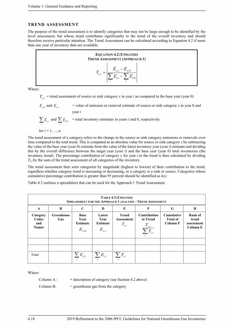
TREND ASSESSMENT The purpose of the trend assessment is to identify categories that may not be large enough to be identified by the level assessment, but whose trend contributes significantly to the trend of the overall inventory and should therefore receive particular attention. The Trend Assessment can be calculated according to Equation 4.2 if more than one year of inventory data are available.
EQUATION 4.2 (UPDATED) TREND ASSESSMENT (APPROACH 1)
, ,0,
, ,0
x t xx t
i t ii i
E ET
E E−
=−∑ ∑
Where:
,x tT = trend assessment of source or sink category x in year t as compared to the base year (year 0)
,0xE and ,x tE = value of emission or removal estimate of source or sink category x in year 0 and year t
,i ti
E∑ and ,0ii
E∑ = total inventory estimates in years t and 0, respectively
for i = 1, ..., n
The trend assessment of a category refers to the change in the source or sink category emissions or removals over time compared to the total trend. This is computed as an absolute value for source or sink category x by subtracting the value of the base year (year 0) estimate from the value of the latest inventory year (year t) estimate and dividing this by the overall difference between the target year (year t) and the base year (year 0) total inventories (the inventory trend). The percentage contribution of category x for year t to the trend is then calculated by dividing Tx,t by the sum of the trend assessment of all categories of the inventory.
The trend assessment then sorts categories by magnitude (highest to lowest) of their contribution to the trend, regardless whether category trend is increasing or decreasing, or a category is a sink or source. Categories whose cumulative percentage contribution is greater than 95 percent should be identified as key.
Table 4.3 outlines a spreadsheet that can be used for the Approach 1 Trend Assessment.
TABLE 4.3 (UPDATED) SPREADSHEET FOR THE APPROACH 1 ANALYSIS – TREND ASSESSMENT
A B C D E F G H
Category Codes and
Names
Greenhouse Gas
Base Year
Estimate
,0xE
Latest Year
Estimate
,x tE
Trend Assessment
,x tT
Contribution to Trend
,
,
x t
i ti
TT∑
Cumulative Total of
Column F
Rank of trend
assessment Column E
Total ,0ii
E∑ ,i t
iE∑
,i ti
T∑
Where:
Column A : = description of category (see Section 4.2 above)
Column B: = greenhouse gas from the category

Chapter 4: Methodological Choice and Identification of Key Categories
2019 Refinement to the 2006 IPCC Guidelines for National Greenhouse Gas Inventories 4.19
Column C: = base year estimate of emissions or removals from the national inventory data, in CO2 equivalent units. Sources and sinks are entered as real values (positive or negative values, respectively)
Column D: = latest year estimate of emissions or removals from the most recent national inventory data, in CO2 equivalent units. Sources and sinks are entered as real values (positive or negative values, respectively)
Column E: = trend assessment from Equation 4.2
Column F: = contribution of the category to the total of trend assessments in last row of Column E, i.e.,
, ,x t i ti
T T∑
Column G: = cumulative total of Column F, calculated after sorting the entries in descending order of magnitude according to Column F
Column H: = rank of the trend assessment value (column E)
The entries in Columns A, B and D should be identical to those in Columns A, B and C in the Table 4.2, for the Approach 1 analysis - Level Assessment. The base year estimate in Column C is always entered, while the latest year estimate in Column D will depend on the year of analysis. The value of Tx,t (which is always positive) should be entered in Column E for each category of sources and sinks, following Equation 4.2, and the sum of all the entries entered in the total line of the table. The percentage contribution of each category to the total of Column E should be computed and entered in Column F. The categories (i.e., the rows of the table) should be sorted in descending order of magnitude, based on Column F. The cumulative total of Column F should then be computed in Column G. Key categories are those that, when summed together in descending order of magnitude, add up to more than 95 percent of the total of Column F. An example of Approach 1 analysis for the level and trend is given in Section 4.5.
The trend assessment treats increasing and decreasing trends similarly. However, for the prioritisation of resources, there may be specific circumstances where countries may not want to invest additional resources in the estimation of key categories with decreasing trends. Underlying reasons why a category showing strong decreasing trend could be key include activity decrease, mitigation measures leading to reduced emission factors or abatement measures (e.g., F-gases, chemical production) changing the production processes. In particular, for a long-term decline of activities (not volatile economic trends) and when the category is not key from the level assessment, it is not always necessary to implement higher tier methods or to collect additional country-specific data if appropriate explanations can be provided why a category may not become more relevant again in the future. This could be the case e.g., for emissions from coal mining in some countries where considerable number of mines are closed or where certain production facilities are shut down. Regardless of the method chosen, countries should endeavour to use the same method for all years in a time series, and therefore it may be more appropriate to continue using a higher tier method if it had been used for previous years.
For other reasons of declining trends such as the introduction of abatement measures or other emission reduction measures, it is important to prioritise resources for the estimation of such categories that were identified as key in the trend assessment. Irrespective of the methodological choice, inventory compilers should clearly and precisely explain and document categories with strongly decreasing trends and should apply appropriate QA/QC procedures.
KEY CATEGORY ANALYSIS FOR A SUBSET OF INVENTORY ESTIMATES Good Practice Guidance for Land Use, Land-Use Change and Forestry (GPG-LULUCF, IPCC 2003) provided guidance on how to conduct a key category analysis using a stepwise approach, identifying first the key (source) categories for the inventory excluding Land Use, Land-Use Change and Forestry (LULUCF), and secondly repeating the key category analysis for the full inventory including the LULUCF categories to identify additional key categories. This two-step approach is now integrated into one general approach. However, inventory compilers may still want to conduct a key category analysis using a subset of inventory estimates. For example, inventory compilers may choose to include only emission sources in order to exclude the effects of removals from the level assessment or in order to exclude the influence of different trends for carbon fluxes from the other emission trends. It is good practice to document the subsets the analysis was performed for and the differences in results comparing with an integrated analysis.
Volume 1: General Guidance and Reporting
4.20 2019 Refinement to the 2006 IPCC Guidelines for National Greenhouse Gas Inventories
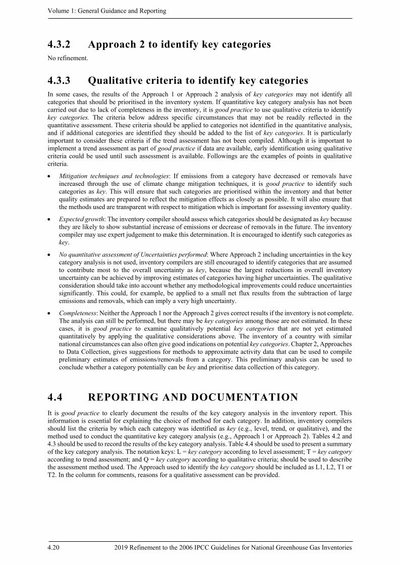
4.3.2 Approach 2 to identify key categories No refinement.
4.3.3 Qualitative criteria to identify key categories In some cases, the results of the Approach 1 or Approach 2 analysis of key categories may not identify all categories that should be prioritised in the inventory system. If quantitative key category analysis has not been carried out due to lack of completeness in the inventory, it is good practice to use qualitative criteria to identify key categories. The criteria below address specific circumstances that may not be readily reflected in the quantitative assessment. These criteria should be applied to categories not identified in the quantitative analysis, and if additional categories are identified they should be added to the list of key categories. It is particularly important to consider these criteria if the trend assessment has not been compiled. Although it is important to implement a trend assessment as part of good practice if data are available, early identification using qualitative criteria could be used until such assessment is available. Followings are the examples of points in qualitative criteria.
• Mitigation techniques and technologies: If emissions from a category have decreased or removals have increased through the use of climate change mitigation techniques, it is good practice to identify such categories as key. This will ensure that such categories are prioritised within the inventory and that better quality estimates are prepared to reflect the mitigation effects as closely as possible. It will also ensure that the methods used are transparent with respect to mitigation which is important for assessing inventory quality.
• Expected growth: The inventory compiler should assess which categories should be designated as key because they are likely to show substantial increase of emissions or decrease of removals in the future. The inventory compiler may use expert judgement to make this determination. It is encouraged to identify such categories as key.
• No quantitative assessment of Uncertainties performed: Where Approach 2 including uncertainties in the key category analysis is not used, inventory compilers are still encouraged to identify categories that are assumed to contribute most to the overall uncertainty as key, because the largest reductions in overall inventory uncertainty can be achieved by improving estimates of categories having higher uncertainties. The qualitative consideration should take into account whether any methodological improvements could reduce uncertainties significantly. This could, for example, be applied to a small net flux results from the subtraction of large emissions and removals, which can imply a very high uncertainty.
• Completeness: Neither the Approach 1 nor the Approach 2 gives correct results if the inventory is not complete. The analysis can still be performed, but there may be key categories among those are not estimated. In these cases, it is good practice to examine qualitatively potential key categories that are not yet estimated quantitatively by applying the qualitative considerations above. The inventory of a country with similar national circumstances can also often give good indications on potential key categories. Chapter 2, Approaches to Data Collection, gives suggestions for methods to approximate activity data that can be used to compile preliminary estimates of emissions/removals from a category. This preliminary analysis can be used to conclude whether a category potentially can be key and prioritise data collection of this category.
4.4 REPORTING AND DOCUMENTATION It is good practice to clearly document the results of the key category analysis in the inventory report. This information is essential for explaining the choice of method for each category. In addition, inventory compilers should list the criteria by which each category was identified as key (e.g., level, trend, or qualitative), and the method used to conduct the quantitative key category analysis (e.g., Approach 1 or Approach 2). Tables 4.2 and 4.3 should be used to record the results of the key category analysis. Table 4.4 should be used to present a summary of the key category analysis. The notation keys: L = key category according to level assessment; T = key category according to trend assessment; and Q = key category according to qualitative criteria; should be used to describe the assessment method used. The Approach used to identify the key category should be included as L1, L2, T1 or T2. In the column for comments, reasons for a qualitative assessment can be provided.

Chapter 4: Methodological Choice and Identification of Key Categories
2019 Refinement to the 2006 IPCC Guidelines for National Greenhouse Gas Inventories 4.21
TABLE 4.4 (UPDATED) SUMMARY OF KEY CATEGORY ANALYSIS
Quantitative method used: Approach 1/Approach 1 and Approach 2 A B C D E
Category Codes Category Names Greenhouse Gas Identification
criteria Comments
Key category analysis is designed to inform the functions of the National Inventory Arrangements and various stakeholders on the priorities for regular update and improvement of the inventory. Therefore, the detailed analysis can be aggregated into a single informative list of the categories identified as key and why as suggested above in Table 4.4. In addition, inventory compilers could consider a means of prioritisation using category rankings across the different analysis. Ideally, this summary should also highlight the tier at which the estimates are estimated to give an indication of the scope for further improvement (see Table 4.4a).
TABLE 4.4A (NEW) KEY CATEGORIES RANKS
A B C D E F
Category Codes and
Names
Greenhouse Gas
Method (Tier)
Latest Year Estimate
[in CO2 eq. units]
Level Assessment Rank
(If Key category)
Trend Assessment Rank
(If Key category)
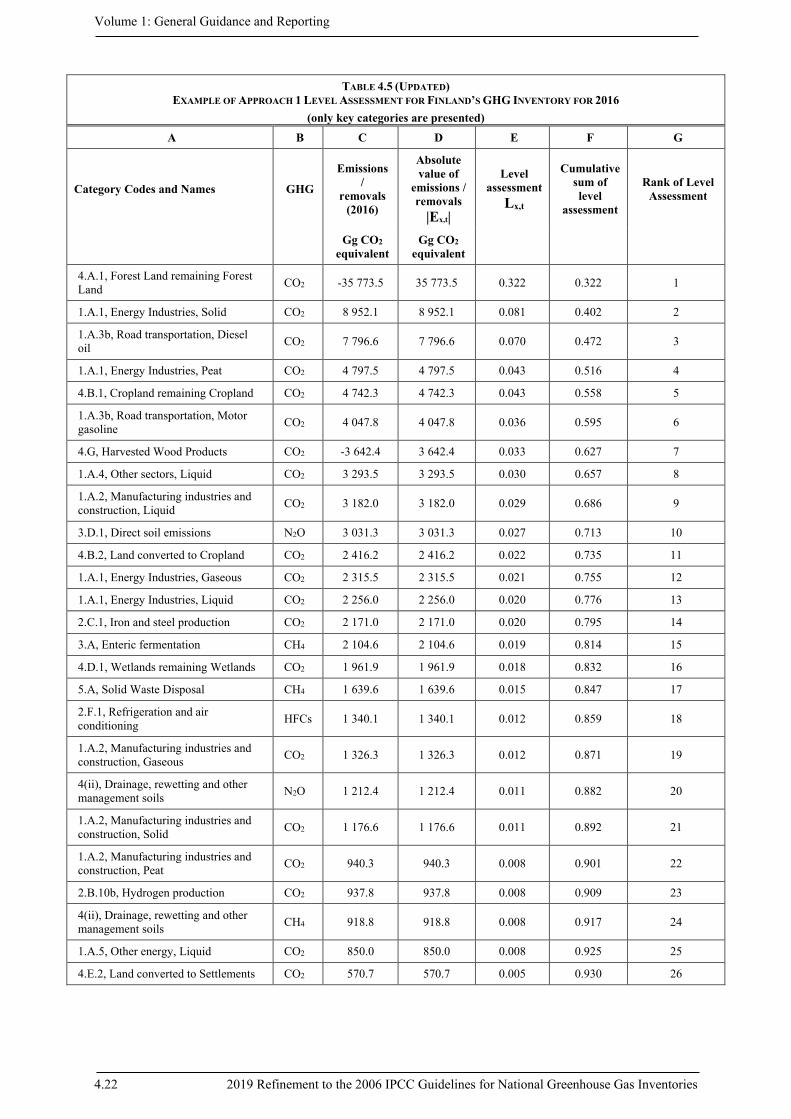
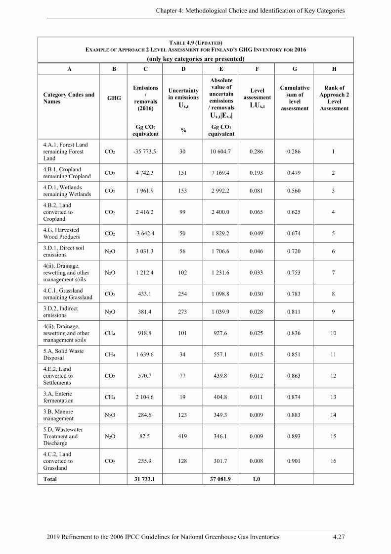
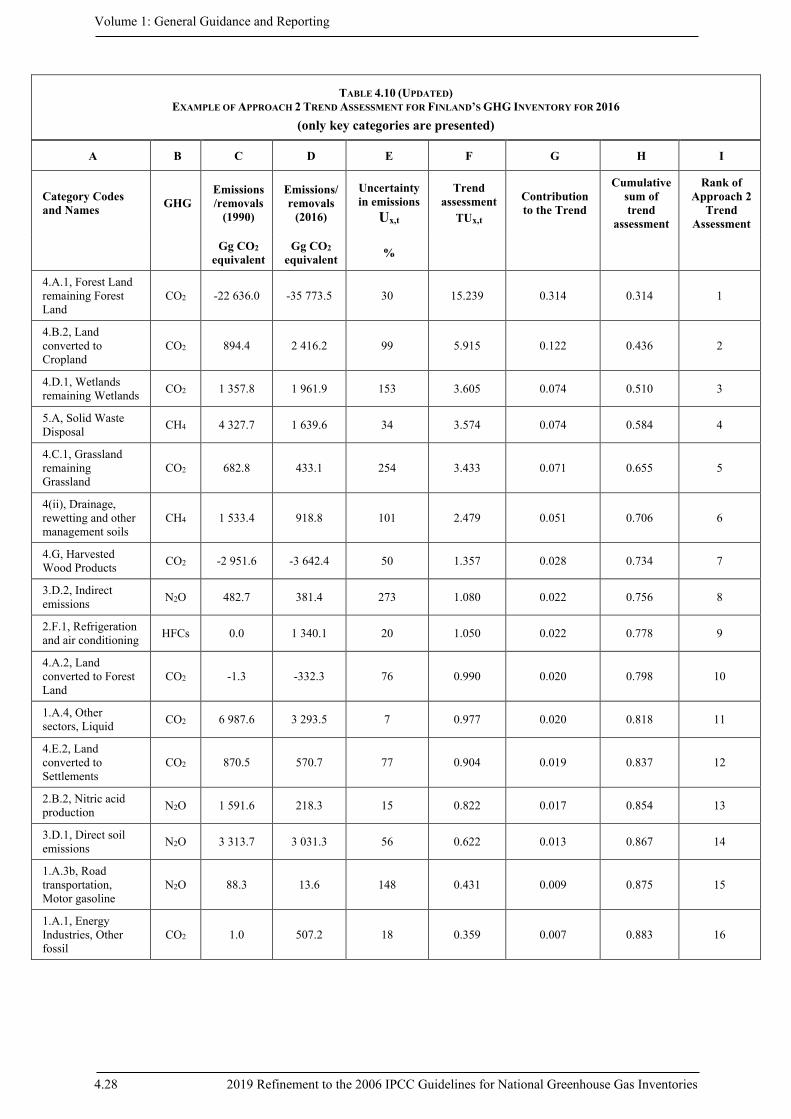
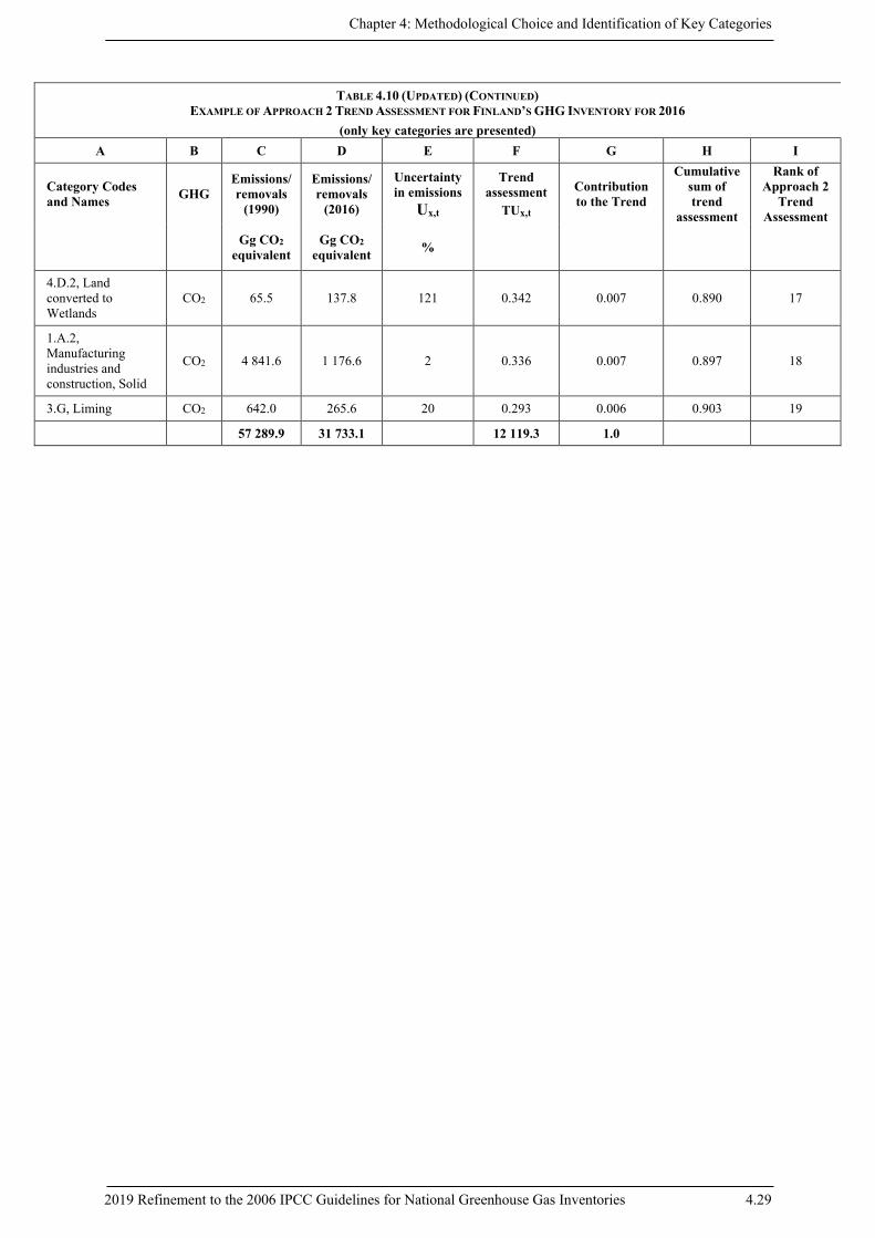
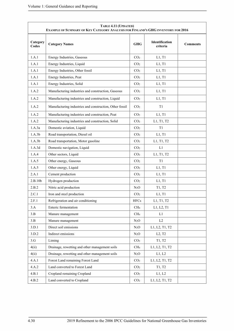
4.5 EXAMPLES OF KEY CATEGORY ANALYSIS The application of the Approach 1 and Approach 2 to Finland's greenhouse gas inventory for the reporting year 2016 is shown in the following tables. Both the level and the trend assessment were conducted using estimates of emissions, removals and uncertainties from the official national inventory of Finland (Statistics Finland, 2018). The category code and the category name (column A in Tables 4.5, 4.6, 4.9-4.11) are presented as reported in the national inventory of Finland. That is why they may not be identical to IPCC category code and name provided in Volume 1, Chapter 8, Table 8.2.
Volume 1: General Guidance and Reporting
4.22 2019 Refinement to the 2006 IPCC Guidelines for National Greenhouse Gas Inventories
TABLE 4.5 (UPDATED) EXAMPLE OF APPROACH 1 LEVEL ASSESSMENT FOR FINLAND’S GHG INVENTORY FOR 2016
(only key categories are presented) A B C D E F G
Category Codes and Names GHG
Emissions /
removals (2016)
Absolute value of
emissions / removals
|Ex,t|
Level assessment
Lx,t
Cumulative sum of level
assessment
Rank of Level Assessment
Gg CO2 equivalent
Gg CO2 equivalent
4.A.1, Forest Land remaining Forest Land CO2 -35 773.5 35 773.5 0.322 0.322 1
1.A.1, Energy Industries, Solid CO2 8 952.1 8 952.1 0.081 0.402 2
1.A.3b, Road transportation, Diesel oil CO2 7 796.6 7 796.6 0.070 0.472 3
1.A.1, Energy Industries, Peat CO2 4 797.5 4 797.5 0.043 0.516 4
4.B.1, Cropland remaining Cropland CO2 4 742.3 4 742.3 0.043 0.558 5
1.A.3b, Road transportation, Motor gasoline CO2 4 047.8 4 047.8 0.036 0.595 6
4.G, Harvested Wood Products CO2 -3 642.4 3 642.4 0.033 0.627 7
1.A.4, Other sectors, Liquid CO2 3 293.5 3 293.5 0.030 0.657 8
1.A.2, Manufacturing industries and construction, Liquid CO2 3 182.0 3 182.0 0.029 0.686 9
3.D.1, Direct soil emissions N2O 3 031.3 3 031.3 0.027 0.713 10
4.B.2, Land converted to Cropland CO2 2 416.2 2 416.2 0.022 0.735 11
1.A.1, Energy Industries, Gaseous CO2 2 315.5 2 315.5 0.021 0.755 12
1.A.1, Energy Industries, Liquid CO2 2 256.0 2 256.0 0.020 0.776 13
2.C.1, Iron and steel production CO2 2 171.0 2 171.0 0.020 0.795 14
3.A, Enteric fermentation CH4 2 104.6 2 104.6 0.019 0.814 15
4.D.1, Wetlands remaining Wetlands CO2 1 961.9 1 961.9 0.018 0.832 16
5.A, Solid Waste Disposal CH4 1 639.6 1 639.6 0.015 0.847 17
2.F.1, Refrigeration and air conditioning HFCs 1 340.1 1 340.1 0.012 0.859 18
1.A.2, Manufacturing industries and construction, Gaseous CO2 1 326.3 1 326.3 0.012 0.871 19
4(ii), Drainage, rewetting and other management soils N2O 1 212.4 1 212.4 0.011 0.882 20
1.A.2, Manufacturing industries and construction, Solid CO2 1 176.6 1 176.6 0.011 0.892 21
1.A.2, Manufacturing industries and construction, Peat CO2 940.3 940.3 0.008 0.901 22
2.B.10b, Hydrogen production CO2 937.8 937.8 0.008 0.909 23
4(ii), Drainage, rewetting and other management soils CH4 918.8 918.8 0.008 0.917 24
1.A.5, Other energy, Liquid CO2 850.0 850.0 0.008 0.925 25
4.E.2, Land converted to Settlements CO2 570.7 570.7 0.005 0.930 26

Chapter 4: Methodological Choice and Identification of Key Categories
2019 Refinement to the 2006 IPCC Guidelines for National Greenhouse Gas Inventories 4.23
TABLE 4.5 (UPDATED) (CONTINUED) EXAMPLE OF APPROACH 1 LEVEL ASSESSMENT FOR FINLAND’S GHG INVENTORY FOR 2016
(only key categories are presented) A B C D E F G
Category Codes and Names GHG
Emissions /
removals (2016)
Absolute value of
emissions / removals
|Ex,t|
Level assessment
Lx,t
Cumulative sum of level
assessment
Rank of Level Assessment
Gg CO2 equivalent
Gg CO2 equivalent
2.A.1, Cement production CO2 553.2 553.2 0.005 0.935 27
1.A.1, Energy Industries, Other fossil CO2 507.2 507.2 0.005 0.940 28
3.B, Manure management CH4 460.9 460.9 0.004 0.944 29
4.C.1, Grassland remaining Grassland CO2 433.1 433.1 0.004 0.948 30
1.A.3d, Domestic navigation, Liquid CO2 403.2 403.2 0.004 0.951 31
Total 31 733.1 111 229.7 1.0
Volume 1: General Guidance and Reporting
4.24 2019 Refinement to the 2006 IPCC Guidelines for National Greenhouse Gas Inventories
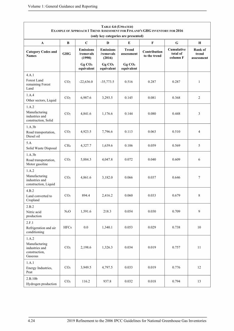
TABLE 4.6 (UPDATED) EXAMPLE OF APPROACH 1 TREND ASSESSMENT FOR FINLAND'S GHG INVENTORY FOR 2016
(only key categories are presented)
A B C D E F G H
Category Codes and Names GHG
Emissions /removals
(1990)
Emissions /removals
(2016)
Trend assessment
Contribution to the trend
Cumulative total of
column F
Rank of trend
assessment
Gg CO2 equivalent
Gg CO2 equivalent
Gg CO2 equivalent
4.A.1 Forest Land remaining Forest Land
CO2 -22,636.0 -35,773.5 0.516 0.287 0.287 1
1.A.4 Other sectors, Liquid
CO2 6,987.6 3,293.5 0.145 0.081 0.368 2
1.A.2 Manufacturing industries and construction, Solid
CO2 4,841.6 1,176.6 0.144 0.080 0.448 3
1.A.3b Road transportation, Diesel oil
CO2 4,923.5 7,796.6 0.113 0.063 0.510 4
5.A Solid Waste Disposal
CH4 4,327.7 1,639.6 0.106 0.059 0.569 5
1.A.3b Road transportation, Motor gasoline
CO2 5,884.3 4,047.8 0.072 0.040 0.609 6
1.A.2 Manufacturing industries and construction, Liquid
CO2 4,861.6 3,182.0 0.066 0.037 0.646 7
4.B.2 Land converted to Cropland
CO2 894.4 2,416.2 0.060 0.033 0.679 8
2.B.2 Nitric acid production
N2O 1,591.6 218.3 0.054 0.030 0.709 9
2.F.1 Refrigeration and air conditioning
HFCs 0.0 1,340.1 0.053 0.029 0.738 10
1.A.2 Manufacturing industries and construction, Gaseous
CO2 2,198.6 1,326.3 0.034 0.019 0.757 11
1.A.1 Energy Industries, Peat
CO2 3,949.5 4,797.5 0.033 0.019 0.776 12
2.B.10b Hydrogen production
CO2 116.2 937.8 0.032 0.018 0.794 13
Chapter 4: Methodological Choice and Identification of Key Categories
2019 Refinement to the 2006 IPCC Guidelines for National Greenhouse Gas Inventories 4.25
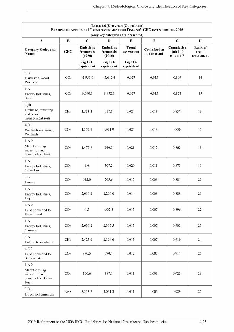
TABLE 4.6 (UPDATED) (CONTINUED) EXAMPLE OF APPROACH 1 TREND ASSESSMENT FOR FINLAND'S GHG INVENTORY FOR 2016
(only key categories are presented) A B C D E F G H
Category Codes and Names GHG
Emissions /removals
(1990)
Emissions /removals
(2016)
Trend assessment
Contribution to the trend
Cumulative total of
column F
Rank of trend
assessment
Gg CO2 equivalent
Gg CO2 equivalent
Gg CO2 equivalent
4.G Harvested Wood Products
CO2 -2,951.6 -3,642.4 0.027 0.015 0.809 14
1.A.1 Energy Industries, Solid
CO2 9,640.1 8,952.1 0.027 0.015 0.824 15
4(ii) Drainage, rewetting and other management soils
CH4 1,533.4 918.8 0.024 0.013 0.837 16
4.D.1 Wetlands remaining Wetlands
CO2 1,357.8 1,961.9 0.024 0.013 0.850 17
1.A.2 Manufacturing industries and construction, Peat
CO2 1,475.9 940.3 0,021 0.012 0.862 18
1.A.1 Energy Industries, Other fossil
CO2 1.0 507.2 0.020 0.011 0.873 19
3.G Liming
CO2 642.0 265.6 0.015 0.008 0.881 20
1.A.1 Energy Industries, Liquid
CO2 2,616.2 2,256.0 0.014 0.008 0.889 21
4.A.2 Land converted to Forest Land
CO2 -1.3 -332.3 0.013 0.007 0.896 22
1.A.1 Energy Industries, Gaseous
CO2 2,636.2 2,315.5 0.013 0.007 0.903 23
3.A Enteric fermentation
CH4 2,423.0 2,104.6 0.013 0.007 0.910 24
4.E.2 Land converted to Settlements
CO2 870.5 570.7 0.012 0.007 0.917 25
1.A.2 Manufacturing industries and construction, Other fossil
CO2 100.6 387.1 0.011 0.006 0.923 26
3.D.1 Direct soil emissions
N2O 3,313.7 3,031.3 0.011 0.006 0.929 27
Volume 1: General Guidance and Reporting
4.26 2019 Refinement to the 2006 IPCC Guidelines for National Greenhouse Gas Inventories
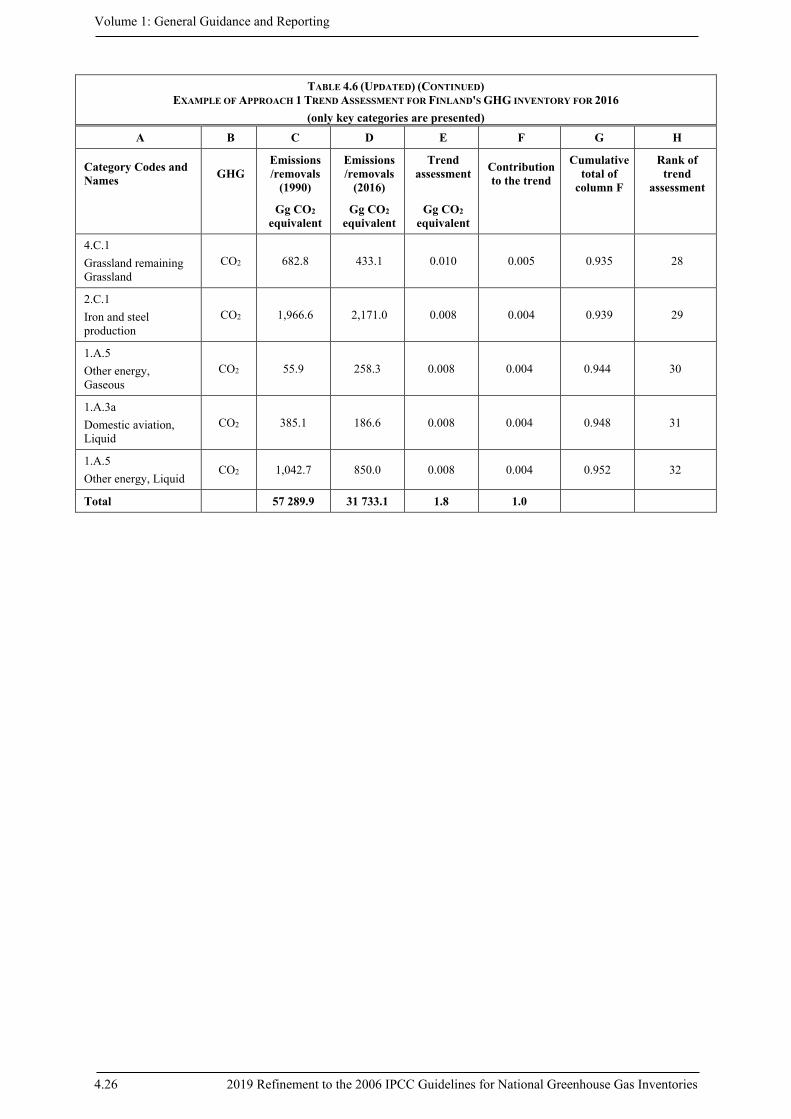
TABLE 4.6 (UPDATED) (CONTINUED) EXAMPLE OF APPROACH 1 TREND ASSESSMENT FOR FINLAND'S GHG INVENTORY FOR 2016
(only key categories are presented) A B C D E F G H
Category Codes and Names GHG
Emissions /removals
(1990)
Emissions /removals
(2016)
Trend assessment
Contribution to the trend
Cumulative total of
column F
Rank of trend
assessment
Gg CO2 equivalent
Gg CO2 equivalent
Gg CO2 equivalent
4.C.1 Grassland remaining Grassland
CO2 682.8 433.1 0.010 0.005 0.935 28
2.C.1 Iron and steel production
CO2 1,966.6 2,171.0 0.008 0.004 0.939 29
1.A.5 Other energy, Gaseous
CO2 55.9 258.3 0.008 0.004 0.944 30
1.A.3a Domestic aviation, Liquid
CO2 385.1 186.6 0.008 0.004 0.948 31
1.A.5 Other energy, Liquid
CO2 1,042.7 850.0 0.008 0.004 0.952 32
Total 57 289.9 31 733.1 1.8 1.0
Chapter 4: Methodological Choice and Identification of Key Categories
2019 Refinement to the 2006 IPCC Guidelines for National Greenhouse Gas Inventories 4.27
TABLE 4.9 (UPDATED) EXAMPLE OF APPROACH 2 LEVEL ASSESSMENT FOR FINLAND’S GHG INVENTORY FOR 2016
(only key categories are presented) A B C D E F G H
Category Codes and Names GHG
Emissions /
removals (2016)
Uncertainty in emissions
Ux,t
Absolute value of
uncertain emissions / removals Ux,t|Ex,t|
Level assessment
LUx,t
Cumulative sum of level
assessment
Rank of Approach 2
Level Assessment
Gg CO2 equivalent % Gg CO2
equivalent
4.A.1, Forest Land remaining Forest Land
CO2 -35 773.5 30 10 604.7 0.286 0.286 1
4.B.1, Cropland remaining Cropland CO2 4 742.3 151 7 169.4 0.193 0.479 2
4.D.1, Wetlands remaining Wetlands CO2 1 961.9 153 2 992.2 0.081 0.560 3
4.B.2, Land converted to Cropland
CO2 2 416.2 99 2 400.0 0.065 0.625 4
4.G, Harvested Wood Products CO2 -3 642.4 50 1 829.2 0.049 0.674 5
3.D.1, Direct soil emissions N2O 3 031.3 56 1 706.6 0.046 0.720 6
4(ii), Drainage, rewetting and other management soils
N2O 1 212.4 102 1 231.6 0.033 0.753 7
4.C.1, Grassland remaining Grassland CO2 433.1 254 1 098.8 0.030 0.783 8
3.D.2, Indirect emissions N2O 381.4 273 1 039.9 0.028 0.811 9
4(ii), Drainage, rewetting and other management soils
CH4 918.8 101 927.6 0.025 0.836 10
5.A, Solid Waste Disposal CH4 1 639.6 34 557.1 0.015 0.851 11
4.E.2, Land converted to Settlements
CO2 570.7 77 439.8 0.012 0.863 12
3.A, Enteric fermentation CH4 2 104.6 19 404.8 0.011 0.874 13
3.B, Manure management N2O 284.6 123 349.3 0.009 0.883 14
5.D, Wastewater Treatment and Discharge
N2O 82.5 419 346.1 0.009 0.893 15
4.C.2, Land converted to Grassland
CO2 235.9 128 301.7 0.008 0.901 16
Total 31 733.1 37 081.9 1.0
Volume 1: General Guidance and Reporting
4.28 2019 Refinement to the 2006 IPCC Guidelines for National Greenhouse Gas Inventories
TABLE 4.10 (UPDATED) EXAMPLE OF APPROACH 2 TREND ASSESSMENT FOR FINLAND’S GHG INVENTORY FOR 2016
(only key categories are presented)
A B C D E F G H I
Category Codes and Names GHG
Emissions/removals
(1990)
Emissions/removals
(2016)
Uncertainty in emissions
Ux,t
Trend assessment
TUx,t
Contribution to the Trend
Cumulative sum of trend
assessment
Rank of Approach 2
Trend Assessment
Gg CO2 equivalent
Gg CO2 equivalent %
4.A.1, Forest Land remaining Forest Land
CO2 -22 636.0 -35 773.5 30 15.239 0.314 0.314 1
4.B.2, Land converted to Cropland
CO2 894.4 2 416.2 99 5.915 0.122 0.436 2
4.D.1, Wetlands remaining Wetlands CO2 1 357.8 1 961.9 153 3.605 0.074 0.510 3
5.A, Solid Waste Disposal CH4 4 327.7 1 639.6 34 3.574 0.074 0.584 4
4.C.1, Grassland remaining Grassland
CO2 682.8 433.1 254 3.433 0.071 0.655 5
4(ii), Drainage, rewetting and other management soils
CH4 1 533.4 918.8 101 2.479 0.051 0.706 6
4.G, Harvested Wood Products CO2 -2 951.6 -3 642.4 50 1.357 0.028 0.734 7
3.D.2, Indirect emissions N2O 482.7 381.4 273 1.080 0.022 0.756 8
2.F.1, Refrigeration and air conditioning HFCs 0.0 1 340.1 20 1.050 0.022 0.778 9
4.A.2, Land converted to Forest Land
CO2 -1.3 -332.3 76 0.990 0.020 0.798 10
1.A.4, Other sectors, Liquid CO2 6 987.6 3 293.5 7 0.977 0.020 0.818 11
4.E.2, Land converted to Settlements
CO2 870.5 570.7 77 0.904 0.019 0.837 12
2.B.2, Nitric acid production N2O 1 591.6 218.3 15 0.822 0.017 0.854 13
3.D.1, Direct soil emissions N2O 3 313.7 3 031.3 56 0.622 0.013 0.867 14
1.A.3b, Road transportation, Motor gasoline
N2O 88.3 13.6 148 0.431 0.009 0.875 15
1.A.1, Energy Industries, Other fossil
CO2 1.0 507.2 18 0.359 0.007 0.883 16
Chapter 4: Methodological Choice and Identification of Key Categories
2019 Refinement to the 2006 IPCC Guidelines for National Greenhouse Gas Inventories 4.29
TABLE 4.10 (UPDATED) (CONTINUED) EXAMPLE OF APPROACH 2 TREND ASSESSMENT FOR FINLAND’S GHG INVENTORY FOR 2016
(only key categories are presented) A B C D E F G H I
Category Codes and Names GHG
Emissions/removals
(1990)
Emissions/removals
(2016)
Uncertainty in emissions
Ux,t
Trend assessment
TUx,t
Contribution to the Trend
Cumulative sum of trend
assessment
Rank of Approach 2
Trend Assessment
Gg CO2 equivalent
Gg CO2 equivalent %
4.D.2, Land converted to Wetlands
CO2 65.5 137.8 121 0.342 0.007 0.890 17
1.A.2, Manufacturing industries and construction, Solid
CO2 4 841.6 1 176.6 2 0.336 0.007 0.897 18
3.G, Liming CO2 642.0 265.6 20 0.293 0.006 0.903 19
57 289.9 31 733.1 12 119.3 1.0
Volume 1: General Guidance and Reporting
4.30 2019 Refinement to the 2006 IPCC Guidelines for National Greenhouse Gas Inventories
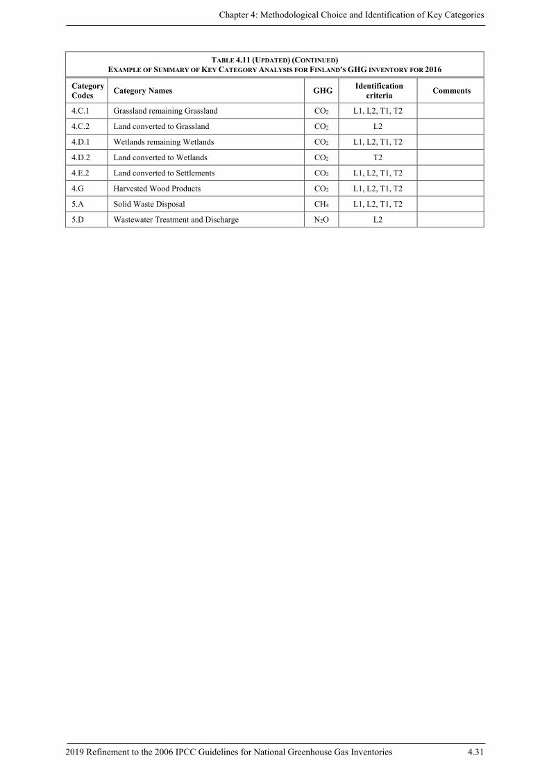
TABLE 4.11 (UPDATED) EXAMPLE OF SUMMARY OF KEY CATEGORY ANALYSIS FOR FINLAND'S GHG INVENTORY FOR 2016
Category Codes Category Names GHG Identification
criteria Comments
1.A.1 Energy Industries, Gaseous CO2 L1, T1
1.A.1 Energy Industries, Liquid CO2 L1, T1
1.A.1 Energy Industries, Other fossil CO2 L1, T1
1.A.1 Energy Industries, Peat CO2 L1, T1
1.A.1 Energy Industries, Solid CO2 L1, T1
1.A.2 Manufacturing industries and construction, Gaseous CO2 L1, T1
1.A.2 Manufacturing industries and construction, Liquid CO2 L1, T1
1.A.2 Manufacturing industries and construction, Other fossil CO2 T1
1.A.2 Manufacturing industries and construction, Peat CO2 L1, T1
1.A.2 Manufacturing industries and construction, Solid CO2 L1, T1, T2
1.A.3a Domestic aviation, Liquid CO2 T1
1.A.3b Road transportation, Diesel oil CO2 L1, T1
1.A.3b Road transportation, Motor gasoline CO2 L1, T1, T2
1.A.3d Domestic navigation, Liquid CO2 L1
1.A.4 Other sectors, Liquid CO2 L1, T1, T2
1.A.5 Other energy, Gaseous CO2 T1
1.A.5 Other energy, Liquid CO2 L1, T1
2.A.1 Cement production CO2 L1, T1
2.B.10b Hydrogen production CO2 L1, T1
2.B.2 Nitric acid production N2O T1, T2
2.C.1 Iron and steel production CO2 L1, T1
2.F.1 Refrigeration and air conditioning HFCs L1, T1, T2
3.A Enteric fermentation CH4 L1, L2, T1
3.B Manure management CH4 L1
3.B Manure management N2O L2
3.D.1 Direct soil emissions N2O L1, L2, T1, T2
3.D.2 Indirect emissions N2O L2, T2
3.G Liming CO2 T1, T2
4(ii) Drainage, rewetting and other management soils CH4 L1, L2, T1, T2
4(ii) Drainage, rewetting and other management soils N2O L1, L2
4.A.1 Forest Land remaining Forest Land CO2 L1, L2, T1, T2
4.A.2 Land converted to Forest Land CO2 T1, T2
4.B.1 Cropland remaining Cropland CO2 L1, L2
4.B.2 Land converted to Cropland CO2 L1, L2, T1, T2
Chapter 4: Methodological Choice and Identification of Key Categories
2019 Refinement to the 2006 IPCC Guidelines for National Greenhouse Gas Inventories 4.31
TABLE 4.11 (UPDATED) (CONTINUED) EXAMPLE OF SUMMARY OF KEY CATEGORY ANALYSIS FOR FINLAND'S GHG INVENTORY FOR 2016
Category Codes Category Names GHG Identification
criteria Comments
4.C.1 Grassland remaining Grassland CO2 L1, L2, T1, T2
4.C.2 Land converted to Grassland CO2 L2
4.D.1 Wetlands remaining Wetlands CO2 L1, L2, T1, T2
4.D.2 Land converted to Wetlands CO2 T2
4.E.2 Land converted to Settlements CO2 L1, L2, T1, T2
4.G Harvested Wood Products CO2 L1, L2, T1, T2
5.A Solid Waste Disposal CH4 L1, L2, T1, T2
5.D Wastewater Treatment and Discharge N2O L2
Volume 1: General Guidance and Reporting
4.32 2019 Refinement to the 2006 IPCC Guidelines for National Greenhouse Gas Inventories
References References copied from the 2006 IPCC Guidelines
IPCC (2000). Good Practice Guidance and Uncertainty Management in National Greenhouse Gas Inventories. Penman, J., Kruger, D., Galbally, I., Hiraishi, T., Nyenzi, B., Emmanuel, S., Buendia, L., Hoppaus, R., Martinsen, T., Meijer, J., Miwa, K., and Tanabe, K. (Eds). Intergovernmental Panel on Climate Change (IPCC), IPCC/OECD/IEA/IGES, Hayama, Japan.
IPCC (2001). Climate Change 2001: The Scientific Basis. Contribution of Working Group I to the Third Assessment Report of the Intergovernmental Panel on Climate Change, Houghton, J.T., Ding, Y., Griggs, D.J., Noguer, M., van der Linden, P.J., Dai, X., Maskell, K. and Johnson, C.A. (eds.), Intergovernmental Panel on Climate Change (IPCC). Cambridge University Press, Cambridge, United Kingdom and New York, NY, USA, 881pp.
IPCC (2003). Good Practice Guidance for Land Use, land-Use Change and Forestry, Penman, J., Gytarsky, M., Hiraishi, T., Kruger, D., Pipatti, R., Buendia, L., Miwa, K., Ngara, T. and Tanabe, K., Wagner, F. (Eds), Intergovernmental Panel on Climate Change (IPCC), IPCC/IGES, Hayama, Japan.
Rypdal, K., and Flugsrud, K. (2001). Sensitivity Analysis as a Tool for Systematic Reductions in GHG Inventory Uncertainties. Environmental Science and Policy. Vol 4 (2-3): pp. 117-135.
Statistics Finland (2005). Greenhouse gas emissions in Finland 1990-2003. National Inventory Report to the UNFCCC, 27 May 2005.
References newly cited in the 2019 Refinement Statistics Finland, 2018. Greenhouse gas emissions in Finland 1990-2016. National Inventory Report under the
UNFCCC and the Kyoto Protocol, 15 April 2018. (https://unfccc.int/documents/65334).