chapter 4 loading and hauling part 1 1ce 417 king saud university

CE 417 King Saud University 1

Chapter 4

Loading and HaulingPart 1


4-1 ESTIMATINGEQUIPMENT TRAVEL TIME

• Cycle time = Fixed time + Variable time (4-1)• Fixed time represents those components of

cycle time other than travel time. It includes:– spot time (moving the unit into position to begin loading), – load time, – maneuver time, and – dump time.

• Fixed time can usually be closely estimated for a particular type of operation.


4-1 ESTIMATINGEQUIPMENT TRAVEL TIME

• Variable time represents the travel time required for a unit to haul material to the unloading site and return.

• It depends on:– the vehicle's weight and power, – the condition of the haul road, – the grades encountered, and – the altitude above sea level.


Rolling Resistance

• It is used to determine the maximum speed of a vehicle in a specific situation.

• The resistance that a vehicle encounters in traveling over a surface is made up of two components:– rolling resistance and – grade resistance.

• Total resistance = Grade resistance + Rolling resistance (4-2)


Rolling Resistance

• Resistance may be expressed in either:– pounds per ton of vehicle weight (kilograms per metric

ton) or in – pounds (kilograms).

• To avoid confusion, the term resistance factor will be used in this chapter to denote resistance in Ib/ton (kg/t).

• Rolling resistance is primarily due to:– tire flexing and – penetration of the travel surface.


Rolling Resistance

• The rolling resistance factor:– for a rubber-tired vehicle equipped with

conventional tires moving over a hard, smooth, level surface = 40 Ib/ton of vehicle weight (20 kg/t).

– For vehicles equipped with radial tires, the rolling resistance factor = 30 Ib/ton (15 kg/t).

– It increases about 30 lb/ton (15 kg/t) for each inch (2.5 cm) of tire penetration.


Rolling Resistance

• This leads to the following equation for estimating rolling resistance factors:– Rolling resistance factor (lb/ton) = 40 + (30 × in.

penetration) (4-3A)– Rolling resistance factor (kg/t) = 20 + (6 × cm

penetration)(4-3B)


Rolling Resistance

• The rolling resistance in pounds (kilograms) = the rolling resistance factor × the vehicle's

weight in tons (metric tons).• Table 4-1 provides typical values for the rolling

resistance factor in construction situations.


TABLE 4-1 Typical values of rolling resistance factor


Rolling Resistance

• Crawler tractors may be thought of as traveling over a road created by their own tracks. – As a result, crawler tractors are usually considered

to have no rolling resistance when calculating vehicle resistance and performance.

• The rolling resistance of crawler tractors does vary somewhat between different surfaces.


Rolling Resistance

• The standard method for rating crawler tractor power (drawbar horsepower) measures the power actually produced at the hitch when operating on a standard surface.– Thus, the rolling resistance of the tractor over the

standard surface has already been subtracted from the tractor's performance.

• The rolling resistance of the towed vehicle must be considered in calculating the total resistance of the combination.


Grade Resistance

• Grade resistance represents that component of vehicle weight which acts parallel to an inclined surface. – When the vehicle is traveling up a grade, grade

resistance is positive. – When traveling downhill, grade resistance is

negative.

5 ft

100 ft

5%100ft 100

ft 5

Grade Resistance


Grade Resistance

• The exact value of grade resistance may be found by multiplying the vehicle's weight by the sine of the angle that the road surface makes with the horizontal.

• For the grades usually encountered in construction, it is sufficiently accurate to use the approximation of Equation 4-4. – Grade resistance factor (lb/ton) =20 × grade (%)

(4-4A)– Grade resistance factor (kg/t) =10 × grade (%)

(4-4B)


Grade Resistance

• That is, a 1% grade (representing a rise of 1 unit in 100 units of horizontal distance) is considered to have a grade resistance equal to 1% of the vehicle's weight. – This corresponds to a grade resistance factor of 20

lb/ton (10 kg/t) for each 1% of grade,


Grade Resistance

• Grade resistance (lb or kg) may be calculated using Equation 4-5 or 4-6.– Grade resistance (lb) = Vehicle weight (tons) ×

Grade resistance factor (lb/ton) (4-5A)– Grade resistance (kg) =Vehicle weight (t) × Grade

resistance factor (kg/t) (4-5B)– Grade resistance (lb) =Vehicle weight (lb) × Grade

(4-6A)– Grade resistance (kg) =Vehicle weight (kg) x Grade

(4-6B)


Effective Grade

• The total resistance to movement of a vehicle – (the sum of its rolling resistance and grade

resistance)– might be expressed in pounds or kilograms.

• OR expressing total resistance is to state it as a grade (%),– A grade resistance equivalent to total resistance

actually encountered.


Effective Grade

• Effective grade may be easily calculated by use of Equation 4-7.– Effective grade (%) = Grade (%) + Rolling resistance

factor (lb/ton)/20 (4-7A) – Effective grade (%) =Grade (%) + Rolling resistance

factor (kg/t)/10 (4-7B)


EXAMPLE 4-1

• A wheel tractor-scraper weighing 100 tons (91 t) is being operated on a haul road with a tire penetration of 2 in. (5 cm).

• What is the total resistance (lb and kg) and effective grade when – (a) the scraper is ascending a slope of 5%; – (b) the scraper is descending a slope of 5%?


EXAMPLE 4-1

• SolutionRolling resistance factor = 40 + (30 × 2) =100 lb/ton

[= 20 + (6 × 5) =50 kg/t]Rolling resistance = 100 (lb/ton) × 100 (tons) = 10,000 lb [= 50 (kg/t) × 91 (t) = 4550 kg](a) Grade resistance = 100 (tons) × 2000 (lb/ton) × 0.05 = 10,000 lb [= 91 (t) x 1000 (kg/t) × 0.05 =4550 kg]Total resistance = 10,000 lb + 10,000 lb = 20,000 lb [= 4550 kg + 4550 kg = 9100 kg]


EXAMPLE 4-1

Effective grade =5 + 100/20 =10%(b) Grade resistance =100 (tons) × 2000(lb/ton)× (-

0.05) = -10,000 lb [= 91 (t) × 1000 (kg/t) x (-0.05) =-4550

kg]Total resistance = -10,000 lb + 10,000 lb = 0 lb

[= -4550 kg + 4550 kg = 0 kg)Effective grade = -5 + 100/20 = 0%

[= -5 + 50/10 = 0%]


EXAMPLE 4-2

• A crawler tractor weighing 80,000 lb (36 t) is towing a rubber-tired scraper weighing 100,000 lb (45.5 t) up a grade of 4%. What is the total resistance (lb and kg) of the combination if the rolling resistance factor is 100 lb/ton (50 kg/t)?


EXAMPLE 4-2

• SolutionRolling resistance (neglect crawler) = 100 000 (lb)

/2000 (lb/ton) × 100 (lb/ton) = 5000 lb[=45.5 (t) × 50 (kg/t) =2275kg]

Grade resistance = 180,000 × 0.04 = 7200 lb (4-6A)[= 81.5 × 1000 kg/t × 0.04 = 3260 kg] (4-6B)

Total resistance = 5000 + 7200 = 12,200 lb[= 2275 + 3260 = 5535 kg] (4-2)


Effect of Altitude

• All internal combustion engines lose power as their elevation above sea level increases because of the decreased density of air at higher elevations.

• Engine power decreases approximately 3% for each 1000 ft (305 m).


Effect of Altitude

• Turbocharged engines are more efficient at higher altitude than are naturally aspirated engines and may deliver full rated power up to an altitude of 10,000 ft (3050 m) or more.


Effect of Altitude

• When derating tables are not available, – the derating factor obtained by the use of Equation

4-8 is sufficiently accurate for estimating the performance of naturally aspirated engines.

– Derating factor (%) = 3 × [(Altitude (ft) - 3000*)/1000 (4-8A)

– Derating factor (%) = (Altitude (m) - 915*)/102 (4-8B)

*Substitute maximum altitude for rated performance, if known.


Effect of Altitude

– The percentage of rated power available= 100 - the derating factor.


Effect of Traction

• The power available to move a vehicle and its load is expressed as :– rimpull for wheel vehicles and – drawbar pull for crawler tractors.


Effect of Traction

• Rimpull is :– the pull available at the rim of the driving wheels

under rated conditions. – Also, the power available at the surface of the

tires.• Drawbar pull is :– the power available at the hitch of a crawler

tractor operating under standard conditions.


Effect of Traction

• Factors affect maximum pull of Vehicle are: a) Operation at increased altitude may reduce the

maximum pull of a vehicle, • as explained in the previous slides.

b) the maximum traction that can be developed between the driving wheels or tracks and the road surface.

Maximum usable pull = Coefficient of traction × Weight on drivers (4-9)

o This represents the maximum pull that a vehicle can develop, regardless of vehicle horsepower


Effect of Traction

• For crawler tractors and all-wheel-drive rubber-tired equipment, – the weight on the drivers is the total vehicle

weight.


TABLE 4-2: Typical values of coefficient of Traction


EXAMPLE 4-3

• A four-wheel drive tractor weighs 44,000 lb (20000 kg) and produces a maximum rimpull of 40,000 lb (18160 kg) at sea level.

• The tractor is being operated at an altitude of 10,000 ft (3050 m) on wet earth.

• A pull of 22,000 lb (10000 kg) is required to move the tractor and its load.

• Can the tractor perform under these conditions? – Use Equation 4-8 to estimate altitude deration.


EXAMPLE 4-3

• SolutionDerating factor = 3 × [(10000 – 3000)/1000]

= 21% (4-8A) [ = (3050 915)/102 =21%] (4-8B)

Percent rated power available=100 21 = 79%Maximum available power = 40,000 × 0.79

= 31,600 lb[ = 18160 × 0.79 = 14346 kg]


EXAMPLE 4-3

Coefficient of traction =0.45 (Table 4-2)Maximum usable pull =0.45 × 44,000 = 19,800lb

(4-9)[= 0.45 × 20000 = 9000

kg]


EXAMPLE 4-3

• Note on Example 4-3:– Because the maximum pull as limited by traction is

less than the required pull, the tractor cannot perform under these conditions.

– For the tractor to operate, it would be necessary to:• reduce the required pull (total resistance), • increase the coefficient of traction, or• increase the tractor's weight on the drivers.


Use of Performance and Retarder Curves

• Crawler tractors may be equipped with direct-drive (manual gearshift) transmissions.

• The drawbar pull and travel speed of this type of transmission are – determined by the gear selected.



• A performance chart indicates: – the maximum speed that a vehicle can maintain under

rated conditions while overcoming a specified total resistance.

• A retarder chart indicates :– the maximum speed at which a vehicle can descend a

slope when the total resistance is negative without using brakes.

– Retarder charts derive their name from the vehicle retarder, which is a hydraulic device used for controlling vehicle speed on a downgrade.



• Figure 4-1 illustrates a relatively simple performance curve of the type often used for crawler tractors. – Rimpull or drawbar pull is shown on the vertical scale

and maximum vehicle speed on the horizontal scale. – The procedure for using this type of curve is to first

calculate the required pull or total resistance of the vehicle and its load (lb or kg).

– Then enter the chart on the vertical scale with the required pull and move horizontally until you intersect one or more gear performance curves.



– Drop vertically from the point of intersection to the horizontal scale.

– The value found represents the maximum speed that the vehicle can maintain while developing the specified pull.

– When the horizontal line of required pull intersects two or more curves for different gears, use the point of intersection farthest to the right, because this represents the maximum speed of the vehicle under the given conditions.


FIGURE 4-1: Typical crawler tractor performance curve.


EXAMPLE 4-4

• Use the performance curve of Figure 4-1 to determine the maximum speed of the tractor when the required pull (total resistance) is 60,000 lb (27240 kg).

• Solution– Enter Figure 4-1 at a drawbar pull of 60,000 lb (27240 kg)

and move horizontally until you intersect the curves for first and second gears.

– Read the corresponding speeds of 1.0 mi/h (1.6 km/h) for second gear and 1.5 mi/h (2.4km/h) for first gear.

– The maximum possible speed is therefore 1.5 mi/h (2.4 km/h) in first gear.



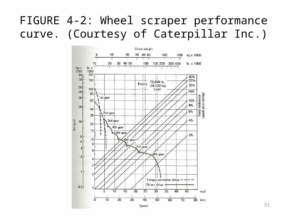
• Figure 4-2 :– represents a more complex performance curve of

the type frequently used by manufacturers of tractor-scrapers, trucks, and wagons.

– In addition to curves of speed versus pull, this type of chart provides a graphical method for calculating the required pull (total resistance).



• To use this type of curve,– Enter the top scale at the actual weight of the

vehicle (empty or loaded as applicable). – Drop vertically until you intersect the diagonal line

corresponding to the percent total resistance (or effective grade), interpolating as necessary.

– From this point move horizontally until you intersect one or more performance curves.

– From the point of intersection, drop vertically to find the maximum vehicle speed.



• When altitude adjustment is required, the procedure is modified slightly. In this case, – start with the gross weight on the top scale and

drop vertically until you intersect the total resistance curve.

– Now, however, move horizontally all the way to the left scale to read the required pull corresponding to vehicle weight and effective grade.



– Next, divide the required pull by the quantity “1 derating factor (expressed as a decimal)” to obtain an adjusted required pull.

– Now, from the adjusted value of required pull on the left scale move horizontally to intersect one or more gear curves and drop vertically to find the maximum vehicle speed.



• This procedure is equivalent to saying that when a vehicle produces only one-half of its rated power due to altitude effects, its maximum speed can be found from its standard performance curve by doubling the actual required pull.

• The procedure is illustrated in Example 4-5.


EXAMPLE 4-5

• Using the performance curve of Figure 4-2, determine the maximum speed of the vehicle if :– its gross weight is 150,000 lb (68000 kg), – the total resistance is 10%, and – the altitude derating factor is 25%.


EXAMPLE 4-5

• Solution– Start on the top scale with a weight of 150,000 lb

(68000 kg), drop vertically to intersect the 10% total grade line, and move horizontally to find a required pull of 15,000 lb (6800 kg) on the left scale.


EXAMPLE 4-5

– Divide 15,000 lb (6800 kg) by 0.75 (1 - derating factor) to obtain an adjusted required pull of 20,000 lb (9080 kg).

– Enter the left scale at 20,000 lb (9080 kg) and move horizontally to intersect the first, second, and third gear curves.

– Drop vertically from the point of intersection with the third gear curve to find a maximum speed of 6 mi/h (10 km/h).


FIGURE 4-2: Wheel scraper performance curve. (Courtesy of Caterpillar Inc.)



• Figure 4-3 illustrates a typical retarder curve. – In this case, it is the retarder curve for the tractor-

scraper whose performance curve is shown in Figure 4-2.

– The retarder curve is read in a manner similar to the performance curve. • Remember, however, that in this case the vertical scale

represents negative total resistance.



• After finding the intersection of the vehicle weight with effective grade,– move horizontally until you intersect the retarder

curve. – Drop vertically from this point to find the

maximum speed at which the vehicle should be operated.


FIGURE 4-3: Wheel scraper retarder curve. (Courtesy of Caterpillar Inc.)


Estimating Travel Time

• The maximum speed that a vehicle can maintain over a section of the haul route cannot be used for calculating travel time over the section, – because it does not include vehicle acceleration

and deceleration.



• One Method for accounting for acceleration and deceleration is:– to multiply the maximum vehicle speed by an average

speed factor from Table 4-3 to obtain an average vehicle speed for the section.

– Travel time for the section is then found by dividing the section length by the average vehicle speed.

– When a section of the haul route involves both starting from rest and coming to a stop, the average speed factor from the first column of Table 4-3 should be applied twice (i.e., use the square of the table value) for that section.



• Second Method for estimating travel time over a section of haul route is :– to use the travel-time curves provided by some

manufacturers. – Separate travel-time curves are prepared for loaded (rated

payload) and empty conditions, as shown in Figures 4-4 and 4-5.

– To adjust for altitude deration when using travel-time curves, multiply the time obtained from the curve by the quantity "1+ derating factor" to obtain the adjusted travel time.


Table 4-3: Average speed factors


FIGURE 4-4: Scraper travel-loaded.(Courtesy of Caterpillar Inc.)


FIGURE 4-5: Scraper travel time-empty. (Courtesy of Caterpillar Inc.)

chapter 4 loading and hauling part 1 1ce 417 king saud university

Documents

resistance resistance

vehicle resistance

rolling resistance factor

grade resistance

total resistance

resistance factor lbton

term resistance factor

fixed time variable