chapter 4 dynamics - field robotics centerfrc.ri.cmu.edu/~alonzo/books/dyn3.pdf · ·...

Chapter 4 Dynamics

Part 3 4.4 Aspects of Linear Systems Theory 4.5 Predictive Modelling and System Identification

Mobile Robotics - Prof Alonzo Kelly, CMU RI 1

Introduction • Nonlinear dynamical systems are the closest thing

to the engineering “theory of everything.” • Applies to:

– growth of bacteria – chemical reactions – financial markets – motion of the planets

• Most important and general model of a mobile robot.


Outline • 4.3 Aspects of Linear Systems Theory

– 4.4.1 Linear Time Invariant Systems – 4.3.2 State Space Representation of Linear Systems – 4.3.3 Nonlinear Dynamical Systems – 4.3.4 Perturbative Dynamics of Linear Systems – Summary

• 4.5 Predictive Modelling and System Identification


Linear Time Invariant ODE s • These are of the form:

• Establishes a relationship between system state x(t) and its derivatives. – Implies that such a system will move (even when u(t)

is not present) – Called a dynamical system


“Forcing Function” “Input”

“Control”

First Order System • Behavior governed by:

• Consider the discrete time equivalent:

• Hence output changes by an amount proportional to the distance-to-go.


“Time Constant”

Step Response • Useful to describe behavior of a

few special inputs. • Step response is response to

constant input applied for t >= 0. • Unforced response. Assume • Substitute into ODE: • Characteristic equation: • The roots of this equation play a

crucial role in determining system behavior.


τs 1+ 0=

Solution • Unforced solution: • Forced solution: • Complete solution: • For we must have • Total Solution:


Solution

• When t=τ, the system has moved …

• … of the total distance to the goal.


Laplace Transform • Extraordinarily powerful for manipulating

compounded ODEs intuitively. • Definition:

• s is a “complex frequency”

• The kernel is a damped sinusoid:


Laplace Transform • For a particular value of s:

• is a (function) dot product with a damped sinusoid.

• y(s) encodes the projections for every value of s. • Its just like a Fourier transform but for complex

frequency s.


Derivatives • Most important property for our purpose:

• Good news!

– Differentiation in the time domain is equivalent to multiplication by s.

• Bad news! – This is why differentiation amplifies noise.


Transforming ODEs • Recall the first order system ODE

• Transform the ODE itself:


ODEs in the time domain become

algebraic eqns in the Laplace domain

Transfer Function • Defined as the ratio of output to input:

• The roots of the characteristic polynomial always appear in the denominator of the transfer function.

• Known as the poles of the system. • An n-th order ODE has n poles.


Characteristic polynomial!

Block Diagrams • ODEs can be represented

graphically as block diagrams.

• Top is time domain, bottom is Laplace domain.


uy+

- ∫ dtτ/1

y

u+

- s/1τ/1

y

y

y

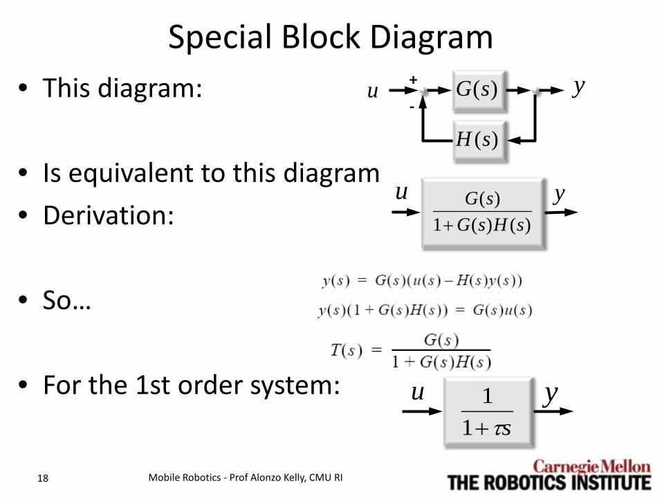
Special Block Diagram • This diagram:

• Is equivalent to this diagram • Derivation:

• So…

• For the 1st order system:


u +

- )(sG y

)(sH

u)()(1

)(sHsG

sG+

y

ysτ+1

1u

Frequency Response • Expresses the gain of the transfer function as

function of frequency: • Substitute into T(s):

• For 1st order system:


Frequency Response

• Huh? Decibels? – dB = 20 log10(amplitude) = 10 log10(power)


Second Order System • One physical manifestation

is a damped oscillator:

• Newton’s second law:

• Rewrite:


Physicists form

Mathematicians form

m f

yc

yk

Simulation • Simulate with:

• Truthoid: You can teach yourself controls if you can write a dynamic simulator like the above.


2nd Order Step Response


2nd Order Step Response • Take Laplace transform of 2nd order ODE:

• Transfer function:

• Behavior depends on the roots of the characteristic equation.


General 1st Order Solution • For the more general 1st order time-varying

system: • The following integrating function exists:

• The general solution therefore is: • When f(t) is constant:


State Space • Remember the special representation used for

Runge Kutta?

• State space = a minimal set of variables which can be used to predict future state given inputs: – Number of initial conditions in a differential equation.


Conversion of an LTI ODE • Consider the second order LTI ODE:

• Choose the state variables to be:


Conversion of an LTI ODE • Rewrite the second and the original ODE as:

• This is of the form:


Example: Damped Oscillator • By inspection:

• Hence, the system is of the form:

• Where x1 is the position and x2 is the velocity.


General Linear Dynamical Systems • State Equations:

• Visualize with:


∫ dtu

dux y

G

F

H+

+

M

+

+

x· t( ) Fx t( ) Gu t( )+=y t( ) Hx t( ) Mu t( )+=

x


∫ dtu

dux y

G

F

H+

+

M

+

+ x

Vector Case – Constant Coefficient • When the system dynamics matrix F(t) is constant

wrt time:

• Recall: by definition (for any matrix A):


Φ t τ,( ) eF t τ–( )=Matrix

Exponential

eA A( )exp I A A 2

2!------ A3

3!------ …+ + + += =

Solution – Vector Case • Knowing the transition matrix is equivalent to

knowing the solution because:

• This is the general solution to:


x t( ) Φ t t0,( )x t0( ) Φ t τ,( )G τ( )u τ( ) τdt0

t

∫+=

x· t( ) F t( )x t( ) G t( )u t( )+=

Vector Convolution

Integral

Nonlinear Dynamical System • Takes the form:


x· t( ) f x t( ) u t( ) t, ,( )=

z t( ) h x t( ) u t( ) t, ,( )=

Nonlinear differential equation

Nonlinear algebraic equation

State Equations System Model Process Model

State Inputs

Forcing Function

Measurement Model Observer

Solutions • Closed form solutions need not exist at all for

nonlinear equations. • With computers though, we can always integrate

like so:

• This case subsumes the linear case so anything true of nonlinear systems is true of a linear one. – Including the next few slides…..


x t( ) x 0( ) f x τ( ) u τ( ) τ, ,( ) τd0

t

∫+=

Relevant Properties • Homogeneity (for some constant k):

• We say system is “homogeneous to degree n wrt u(t)”.

• u(t) must occur in f() as a factor like so:

• As a result, all terms of the Taylor series of f() over u(t) of order less than n vanish.


f x t( ) k u× t( ),[ ] kn f x t( ) u t( ),[ ]×=

f x t( ) u t( ),[ ] un t( )g x t( )( )=

Drift Free • All homogeneous systems are drift free.Their zero

input response is zero.

• Such systems can be stopped instantly by nulling the inputs.

• Similar to “drift-free” designation in control theory.


u t( ) 0 x· t( )⇒ 0= =

Reversibility & Monotonicity • Odd degree homogeneity implies a reversible

system.

• Even degree homogeneity implies monotonicity. Sign of derivative irrelevant to sign of u().


u2 t( ) u1 τ t–( )–= f2 t( )⇒ f1 τ t–( )–=

u2 t( ) u1 t( )–= f2 t( )⇒ f1 t( )=

Linearizing a Nonlinear Diff Eq • Consider again:

• Suppose some u(t) generates some solution x(t). This is

the “reference trajectory”. • Suppose we want a solution for:

• The solution can be written as:

• Defines the state perturbation dx(t) as the difference in

solutions.


x· t( ) f x t( ) u t( ) t, ,( )=

u' t( ) u t( ) δu t( )+=

x' t( ) x t( ) δx t( )+=

input perturbation

state perturbation

perturbed input

perturbed state

Linearizing a Nonlinear Diff Eq • If the perturbed solution is a solution, then:

• Write a truncated Taylor Series at each point in

time for the derivative f():

• Where the two new matrices are the Jacobians:


x'· t( ) x· t( ) δx· t( )+ f x t( ) δx t( )+ u t( ) δu t( )+ t, ,[ ]= =

f x t( ) δx t( )+ u t( ) δu t( )+ t, ,[ ] f x t( ) u t( ) t, ,[ ] F t( )δx t( ) G t( )δu t( )+ +≈

F t( )x∂

∂ fx u,

= G t( )u∂∂ f

x u,

=

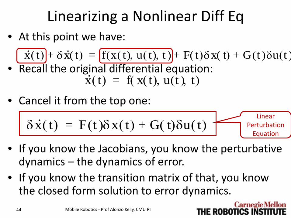
Linearizing a Nonlinear Diff Eq • At this point we have:

• Recall the original differential equation:

• Cancel it from the top one:

• If you know the Jacobians, you know the perturbative dynamics – the dynamics of error.

• If you know the transition matrix of that, you know the closed form solution to error dynamics. Mobile Robotics - Prof Alonzo Kelly, CMU RI 44

x· t( ) δx· t( )+ f x t( ) u t( ) t, ,( ) F t( )δx t( ) G t( )δu t( )+ +=

x· t( ) f x t( ) u t( ) t, ,( )=

δx· t( ) F t( )δx t( ) G t( )δu t( )+=Linear

Perturbation Equation

Next year • Move slide 60 (or so) on perturbative dynamics od

State Est 1 here. The example will be used later in State Est1 to derive Integrated Heading error dynamics in dead reckoning.

• Also move slide 61, 62 on transition matrix.


Summary • Nonlinear dynamical systems cannot be solved in

closed form in general. • The general solution for linear, even time-varying,

dynamical systems exists. – Solution rests on Transition matrix

• Perturbative techniques linearize nonlinear differential equations – makes them solveable.


Outline • 4.3 Aspects of Linear Systems Theory • 4.5 Predictive Modelling and System Identification


Introduction – the “ives” • Mobile robots must often be:

– Deliberative – decide among options – Perceptive – aware of the surroundings – Reactive – capable of fast action

• They must be both – smart and – fast

• … doing that involves tradeoffs.


Role of Dynamics • In support of the above, need to be …

– Predictive – able to project consequences – Active – able to execute a plan of action

• You need dynamics models for both of these.


Predictive Modeling • Must model …

– Information processing and propagation. – Physical vehicle / environment interaction.

• Often need to map …

– what you can do (exert forces) – what you care about (trajectory through space).

• Latter requires integrating the dynamics.



– 4.5.1 Braking – 4.5.2 Turning – 4.5.3 Vehicle Rollover – 4.5.4 Wheel Slip and Yaw Stability – 4.5.5 Parameterization and Linearization of Dynamic

Models – 4.5.6 System Identification – Summary


Reasons for Braking • A) Last resort response to problems.

– Collision is imminent due to • no solution or • inadequate planning or control.

• B) Deliberately slow down. – On slopes – The motion is finished. – In order to turn around.


Avoiding Collision • Requires precise knowledge of the time and space

required to react.

• These depend heavily on: – Speed (initial KE) – Friction (work done by friction) – Slope (change in PE)


Why Care about time?

Braking Model • Assume brakes are applied instantly: • Free body diagram:

– Friction and Weight are coupled.

• Do heavier vehicles take longer to stop?

55 Mobile Robotics - Prof Alonzo Kelly, CMU RI

Simple Model • Equate work done by external forces to initial

Kinetic energy (assume it is all used up).

• Solve for braking distance:

• Do heavier vehicles take more distance to stop?


12---mv2 µsmgsbrake=

s brakev2

2µ sg------------=

Tangent: Falling • Do heavier objects fall faster?


Leaning Tower

small object

large object

Impact of Slopes • Again equate work

done to initial KE:

• Solve for distance: • Effective coefficient

of friction: • Then, simply:


12---mv2 µsmgcθ mgsθ–( )sbrake=

sbrakev2

2g µscθ sθ–( )-----------------------------------=

µef f µscθ sθ–( )=

sb rakev2

2µef fg---------------=

Simple Model on Slopes • Critical angle exists

beyond which gravity overcomes friction….

• Atan() is highly nonlinear.


µs cθ sθ– 0 θtan⇒ µ s= =

General Case • More generally:

• Robots can compute this. – The terrain shape is known. – Keep integrating until KE exhausted. – Final value of s is stopping distance.


F sd•

0

s

∫ 12---mv2=

Rough Heuristic for Slopes • Make small angle assumptions:

• Change in effective coefficient:

• Ratio of sloped to level stopping distance:

• Stopping distance increases or decreases by the factor


cθ 1= sθ θ=

µef f θ( ) µs cθ sθ–( ) µs θ–≈=

10% slope reduces µ by 0.1

sθ

s0---- 1

1 θµ s-----–

-------------- 1 θµs-----+≈=

θ µ s⁄

Turning • Goal is to cause terrain to exert a moment on the

vehicle – By 3rd law, vehicle must exert a moment on the

terrain.

• May actuate: – Wheel steering (Ackerman) – Wheel speeds (Differential, skid)


Simple Motion Prediction • For small steer angles:

• Integrate the differential equations using “back

substitution”:

• Errors in steering are integrated twice to determine errors in predicted position.


κ t( ) α t( )=

θ t( ) θ0 V t( )α t( )dt0

t

∫+=

x t( ) x0 V t( ) θ t( )( )dtcos0

t

∫+=

y t( ) y0 V t( ) θ t( )( )sin dt0

t

∫+=

Note mapping from inputs to outputs are

integrals.

The mapping from steer angle and

velocity onto the path the robot

follows. Assumes flat terrain.

Reverse Turn @ Multiple Speeds • A curvature step is the

most ambitious maneuver.

• Not modeling steering response leads to collisions with obstacles above 3.5 m/sec speed.


• One Curvature • Various Speeds

“Reverse Turn”

Recall: Speed Coupling • Due to vehicle

dynamics…….

• The path followed is generally a function of speed.

• Therefore, they must be estimated together.


Reverse Turn @ Multiple Curvatures • Different steering

commands. Same speed (5 m/s).

• It takes a long distance to cross the forward (y) axis. – Its longer the faster

you are going.


• One Speed • Various Curvatures

“Reverse Turn”

Swerving • Recall our typical 2D equations of motion:


Swerving • Assuming velocity is constant, and

curvature rate is limited and constant, the yaw is given by:

• This gives the position coordinates as:


“Clothoids”

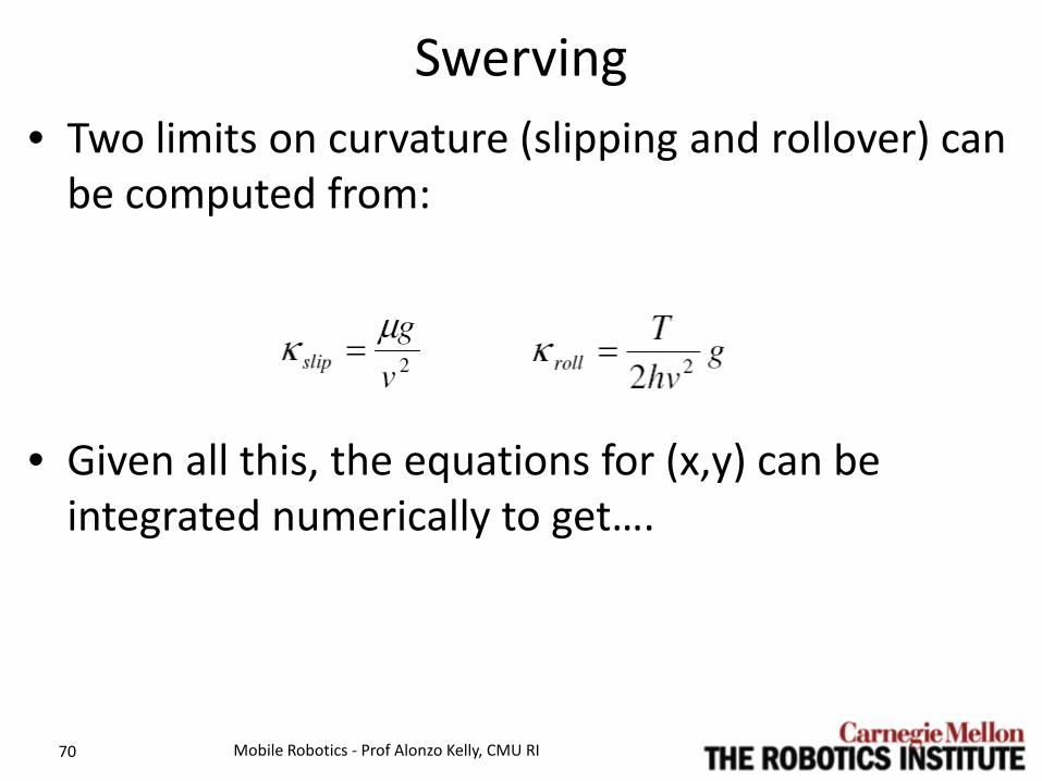
Swerving • Two limits on curvature (slipping and rollover) can

be computed from:

• Given all this, the equations for (x,y) can be integrated numerically to get….


Swerving (Urmson)


1) Roughly linear!

2) Lower than stopping distance (v^2/10) at 10 m/s and beyond

Sometimes you can swerve in

time even when you cannot stop.

Note • There is plenty of content on rollver in dyn1 too.

Check it all/


Field Robots Motivation • Contemporary

mining, forestry, agriculture, and military vehicles, operate – on slopes and/or – at high speeds

• Field robots do rollover! – They at least need a

reactive system if predictive elements fail.


Industrial Robots Motivation • Market forces

reward manufacturers of industrial truck that: – Are narrower, – Lift heavier loads, – Lift them higher.

• Automated industrial trucks face the same challenges.


Center of

Gravity

PerceptOR - Yuma


• Some Robots live dangerously. • Listen for the distinctive “Crunch” of a ladar

sensor.

UGCV – Roll Test


Lift Truck Simulations


Ungoverned Governed

Rollover • More likely in factory and field robots. • Happens due to combinations of:

– narrow wheel spacing, – high centers of gravity – high inertial forces (speeds and curvatures) – steep slopes

• Incidents may be: – Terrain induced (slide sideways into a curb) – Maneuver induced (turn too sharp on a hill)


Examples • Tipover when stopping on

a downslope.

• Rollover when turning sharply.


Forms of Instability • Must distinguish two events:

– Point of wheel liftoff (still recoverable) – Point were cg passes over wheels (irrecoverable)

• The first occurs first and is easier to detect – Does not require knowledge of inertia.


NOTE • The book was updated to use a singel figure and

to not reverse the direction of the reactions as the figures do here.

• That changed the signs in a few places so the figures and the math need to be updated here to be consistent with the book.


Static Case • For translational equilibrium:

• For rotational equilibrium:


fyufyl

+ mg φsin=

fzufzl

+ mg φcos=

fzut mg φhsin+ mg φ t

2---cos=

Sum moments about lower wheel. Do cross products (r x f) in body coordinates where it is easy

t

Static Liftoff • Imagine raising the slope:

– fzu decreases – fzl increases

• At some point fzu=0 and the moment balance becomes:

• Can solve for the slope at which tipping occurs:

• Using this, can compute cg height using a tilt table.


mg φhsin mg φ t2---cos=

φtan t2h------=

An important/famous vehicle design parameter affecting stability.

Gravity is the only force involved.

mg

mgsφ

mgcφ

Static Liftoff • Since we are talking about

a moment of a single force… – Result can be understood

in terms of the direction of gravity.

• Liftoff criterion is first satisfied when gravity vector: – emanating from the center

of gravity (cg) – points at the lower wheel

contact point. Mobile Robotics - Prof Alonzo Kelly, CMU RI 88

Dynamic Case • Use D’Alemberts principle:

– I.E. treat – ma like a real force.

• Moment balance:

• Solve for lateral acceleration in g’s:

• Set to get lateral acceleration threshold.


fz it– mayh– mgsφh mgc φ t

2---+ + 0=

ayg----- t

2---cφ hsφ

tfzi

mg--------–+ h⁄=

fzi0= ay

g----- t

2---cφ hsφ+ h⁄=

Vehicle is turning left Ma is reversed in sense

per D’Alembert

Dynamic Case • Rewrite last result:

• Liftoff when net noncontact specific force:

• Points at the outside wheel contact point. • A pendulum mounted at the cg aligns with this

vector.


ay gsφ–gcφ

-------------------- t2h------=

f g a–=

Interpretations • Static case is just special case of dynamic (ay=0) • Stability increases with:

– Lower cg h – Wider tread t – Lowering slope – Decreasing acceleration

• Slowing down • Reducing curvature


ay gsφ–gcφ

-------------------- t2h------=

Stability Pyramid • Theory generalizes to vehicles of any shape. • Stability pyramid = the pyramid formed with the

wheel contact points with the cg at the apex. • Each edge is a potential tipover axis.

– Moment is: – Unbalanced when:


Wheels need not be in the same

plane.

M r f ×=

M a• 0>

Implementation • Some vehicles articulate mass so the cg would

have to be (re-)calculated in real time. • An accelerometer or inclinometer works like a

pendulum, but: – It probably cannot be placed at the cg. – So, acceleration transforms are necessary.


Slip Angle • Defined for a car as:

• Alternatively using body frame velocity

components:

• Can be defined for wheels too.


ζ

ψ β ψ ζ–=

β 2 Vy Vx,( )atan=

Generalized Slip Angle • Define the angle between the actual and intended

velocity:


ζ

ψ

actual reference

β V V⋅( ) V V( )⁄[ ]acos=

Generalized Slip Equation • The velocity may be incorrect in all 3 degrees of

freedom. • Express errors in body coordinates:


ζ

ψ

x·

y·

θ·

cθ sθ– 0sθ cθ 00 0 1

Vx

Vy

ω

δV x

δV y

δω

+

=

Vw

R θ( ) V δV+( )=

actual reference

Wheel Slip Graphs


0.00

-0.05

-0.10

-0.15

-0.20

-0.25 0.2 0.4 0.6 0.8 1.0 1.2

δω (r

ads/

sec)

V (m/sec)

κ=0.4

κ=0.5

κ=0.6

0.25

0.20

0.15

0.10

0.05

0.0 0.2 0.4 0.6 0.8 1.0 1.2

V (m/sec)

κ=0.4 κ=0.5 κ=0.6

δVy (

m/s

ec)

0.00

-0.05

-0.10

-0.15

-0.20

-0.25 0.2 0.4 0.6 0.8 1.0 1.2

V (m/sec)

κ=0.4 κ=0.5 κ=0.6

δVx (

m/s

ec)

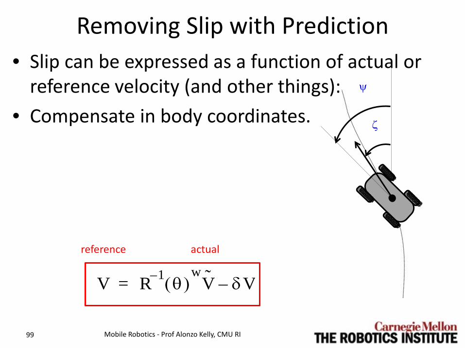
Removing Slip with Prediction • Slip can be expressed as a function of actual or

reference velocity (and other things): • Compensate in body coordinates.


ζ

ψ

V R 1– θ( ) Vw

δV–=

actual reference

Outline • Introduction • Wheel Slip • Braking • Turning & Swerving • Rollover • System Identification • Summary



System (dynamics)

System Model

Input

u

Output

y

Noise υ

Measurements z

Parameter Estimation

Prediction Error

z - y

Output prediction

y

Parameter Updates


Side Slip

Summary • Braking distance:

– increases quadratically with initial speed – depends heavily on slope

• Turning and Swerving: – predicting steering maneuvers requires calibrated

dynamic models.

• Rollover stability can be measured with a pendulum at the cg.


chapter 4 dynamics - field robotics centerfrc.ri.cmu.edu/~alonzo/books/dyn3.pdf · ·...

Documents