chapter 10 motion planning - field robotics centerfrc.ri.cmu.edu/~alonzo/books/plan2.pdf · global...
TRANSCRIPT
Chapter 10 Motion Planning
Part 2 10.2 Representation and Search for Global Motion Planning
Mobile Robotics - Prof Alonzo Kelly, CMU RI 1

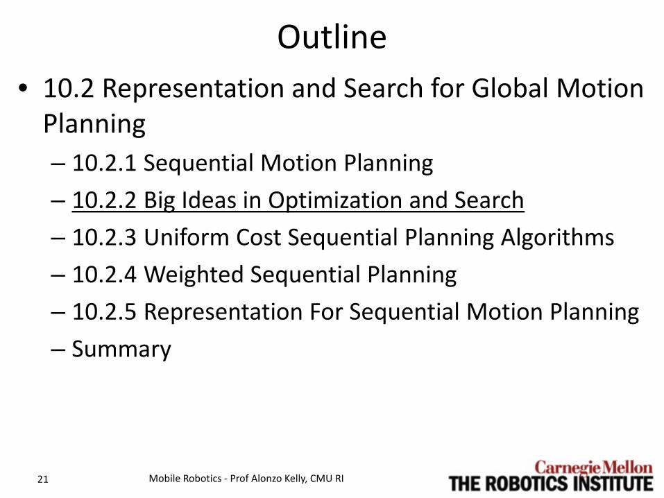
Outline • 10.2 Representation and Search for Global Motion
Planning – 10.2.1 Sequential Motion Planning – 10.2.2 Big Ideas in Optimization and Search – 10.2.3 Uniform Cost Sequential Planning Algorithms – 10.2.4 Weighted Sequential Planning – 10.2.5 Representation For Sequential Motion Planning – Summary
Mobile Robotics - Prof Alonzo Kelly, CMU RI 2

Solution Techniques • Recall: Path planning is essentially an optimal
control problem. • Three clear solution techniques for optimal
control: – Parameterization (how we did trajectory generation) – Variational (“geodesics”). – Dynamic Programming
• Why not just use trajectory generation algorithms? – We shall see….
Mobile Robotics - Prof Alonzo Kelly, CMU RI 3

Outline • 10.2 Representation and Search for Global Motion
Planning – 10.2.1 Sequential Motion Planning – 10.2.2 Big Ideas in Optimization and Search – 10.2.3 Uniform Cost Sequential Planning Algorithms – 10.2.4 Weighted Sequential Planning – 10.2.5 Representation For Sequential Motion Planning – Summary
Mobile Robotics - Prof Alonzo Kelly, CMU RI 4

10.2.1.1 Why Not Continuum Methods? • Too Many Solutions…
– Scale is much larger. Many more solutions in some funny continuum sense.
• Too many Constraints… – Avoiding 1000 obstacles is 1000 constraints.
• Too many local minima.
Mobile Robotics - Prof Alonzo Kelly, CMU RI 5
S G
Two decisions, each with 2 choices leads to 4 homotopically distinct paths.

10.2.1.2 Discretization of Search Spaces • Embed a network in space and search it (instead
of space itself)..
Mobile Robotics - Prof Alonzo Kelly, CMU RI 6
S G

10.2.1.2 Discretization of Search Spaces (State Discretization)
• Discrete states may or may not be regularly arranged.
• Join nearby states with edges.
• Produces a graph embedded in (i.e. a subset of) workspace or C space.
• Planning paths … – in the continuum
• … has become … – reduced to a graph search
problem. Mobile Robotics - Prof Alonzo Kelly, CMU RI 7
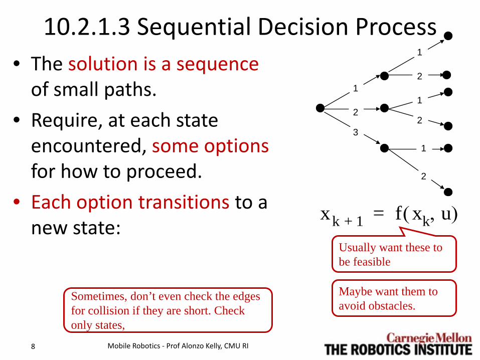
10.2.1.3 Sequential Decision Process • The solution is a sequence
of small paths. • Require, at each state
encountered, some options for how to proceed.
• Each option transitions to a new state:
Mobile Robotics - Prof Alonzo Kelly, CMU RI 8
3
2
1
1
1
1
2
2
2
xk 1+ f xk u,( )=Usually want these to be feasible
Maybe want them to avoid obstacles.
Sometimes, don’t even check the edges for collision if they are short. Check only states,

Discrete Motion Planning Formulation • Given:
– a graph – a start state – a goal state
• Find a sequence of edges (equivalently, states) connecting start to goal.
• Some formulations have multiple goals or goal regions.
• Some have multiple start states (uncertainty).
Mobile Robotics - Prof Alonzo Kelly, CMU RI 9
S
G

10.2.1.4 World Model, C-Space, and Search Graph (Discrete Representations)
• Convenient for performing sequential search. • Abstract the continuum in two ways: • 1) Discretize the state space • 2) Discretize the motions so that they connect
only the (nearby) states. • Sometimes we do this based on knowledge of:
– neither obstacle nor mobility (grid) – mobility ignoring obstacles (state lattice) – obstacles ignoring mobility (Voronoi diagram,
roadmaps) Mobile Robotics - Prof Alonzo Kelly, CMU RI 11

10.2.1.4 World Model, C-Space, and Search Graph (Grids & Lattices as Graphs)
• Search algorithms defined on networks.
• Grids and lattices are just regular arrangements of states.
• ANY algorithm defined on a network can be implemented on a grid.
• Edges may be implicit but they are always there.
Mobile Robotics - Prof Alonzo Kelly, CMU RI 12
=

10.2.1.5 Search Space Design • Implicit edges defer the motion generation problem
post-planning. – Works sometimes. System must be predictable. – However, sometimes constraints must be represented to
avoid failure. • Tradeoff is search convenience vs constraint
convenience. • Discrete obstacles can be encoded in search space.
– by removing edges. – Otherwise, need cost field.
• Often search space is generated on the fly but in rare cases, like a real road network, its known beforehand….
Mobile Robotics - Prof Alonzo Kelly, CMU RI 14
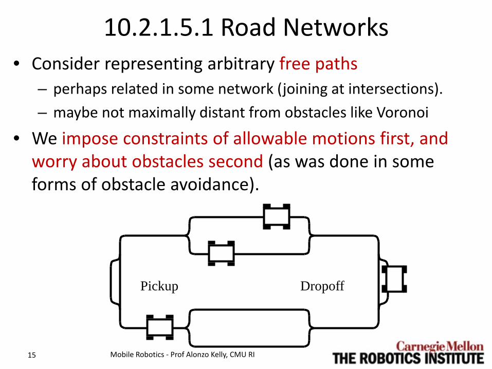
10.2.1.5.1 Road Networks • Consider representing arbitrary free paths
– perhaps related in some network (joining at intersections). – maybe not maximally distant from obstacles like Voronoi
• We impose constraints of allowable motions first, and worry about obstacles second (as was done in some forms of obstacle avoidance).
Mobile Robotics - Prof Alonzo Kelly, CMU RI 15
Pickup Dropoff
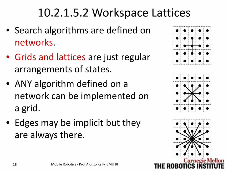
10.2.1.5.2 Workspace Lattices • Search algorithms are defined on
networks. • Grids and lattices are just regular
arrangements of states. • ANY algorithm defined on a
network can be implemented on a grid.
• Edges may be implicit but they are always there. Mobile Robotics - Prof Alonzo Kelly, CMU RI 16

10.2.1.5.3 State Lattices • Enforce differential constraints directly in the
searce space. • For example, Reeds-Shepp car. Require heading
continuity across nodes.
Mobile Robotics - Prof Alonzo Kelly, CMU RI 17

10.2.1.5.4 Voronoi Diagrams • Set of all points which are
equidistant from at least two obstacle boundaries.
• Local maxima in the proximity field.
• Can be generated from a field representation with the “distance transform”.
Mobile Robotics - Prof Alonzo Kelly, CMU RI 18
Goal
Obstacle Obstacle
Robot Obstacle
Outline • 10.2 Representation and Search for Global Motion
Planning – 10.2.1 Sequential Motion Planning – 10.2.2 Big Ideas in Optimization and Search – 10.2.3 Uniform Cost Sequential Planning Algorithms – 10.2.4 Weighted Sequential Planning – 10.2.5 Representation For Sequential Motion Planning – Summary
Mobile Robotics - Prof Alonzo Kelly, CMU RI 21
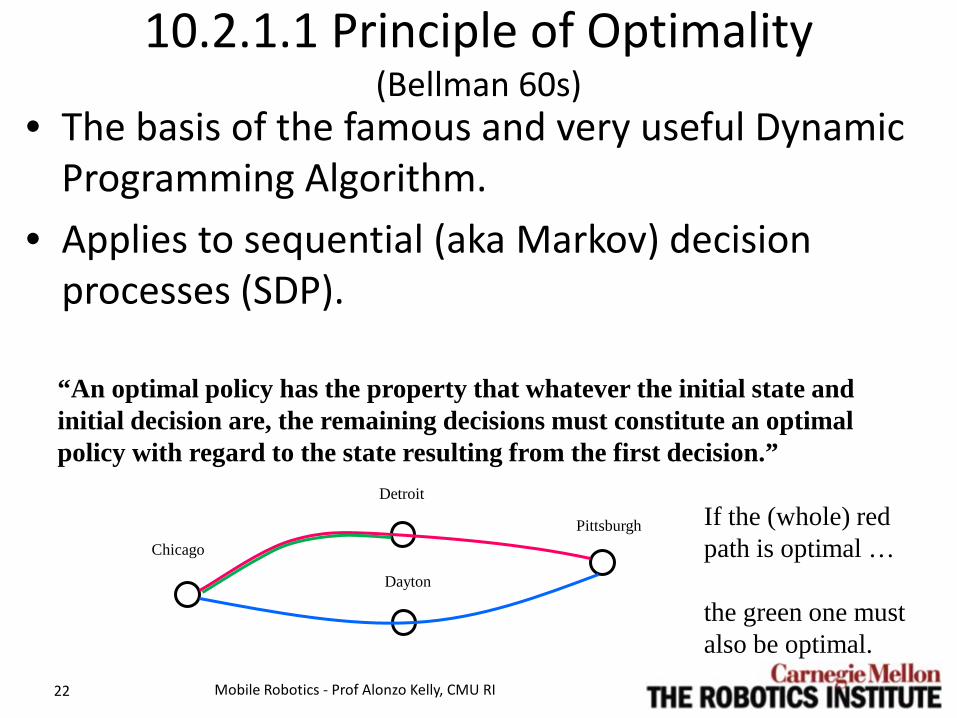
10.2.1.1 Principle of Optimality (Bellman 60s)
• The basis of the famous and very useful Dynamic Programming Algorithm.
• Applies to sequential (aka Markov) decision processes (SDP).
Mobile Robotics - Prof Alonzo Kelly, CMU RI 22
“An optimal policy has the property that whatever the initial state and initial decision are, the remaining decisions must constitute an optimal policy with regard to the state resulting from the first decision.”
If the (whole) red path is optimal … the green one must also be optimal.
Pittsburgh Chicago
Detroit
Dayton
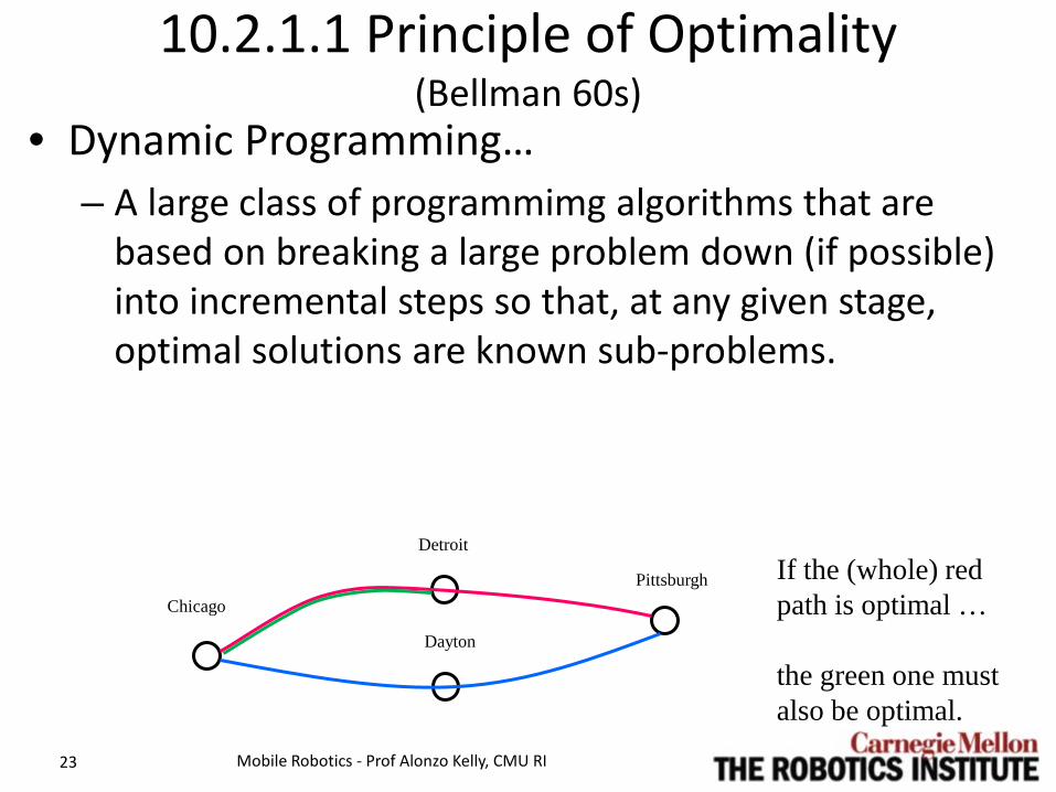
10.2.1.1 Principle of Optimality (Bellman 60s)
• Dynamic Programming… – A large class of programmimg algorithms that are
based on breaking a large problem down (if possible) into incremental steps so that, at any given stage, optimal solutions are known sub-problems.
Mobile Robotics - Prof Alonzo Kelly, CMU RI 23
If the (whole) red path is optimal … the green one must also be optimal.
Pittsburgh Chicago
Detroit
Dayton

10.2.1.1 Principle of Optimality (Notion of Proof)
• Intuitively, the optimal solution to the entire problem must be composed of optimal solutions to the subproblems. – This only true for SDPs.
• Easy to prove by contradiction….. – Otherwise, you could substitute the optimal
subproblem and generate a better solution.
Mobile Robotics - Prof Alonzo Kelly, CMU RI 24
Pittsburgh Chicago
Detroit
Dayton

10.2.1.1 Principle of Optimality (Dynamic Programming)
• Starting at the start node, the mouse has to pick one of 3 and then one of (2 or 3) nodes…
• There are 7 possible paths of 3 edges (7 edges in middle phase).
Mobile Robotics - Prof Alonzo Kelly, CMU RI 25
Cheese
1
3
2
3
1
1
3
2 3
3
4
4 5
Mouse

10.2.2.1.1 Backward Traversal • To solve the problem, work backwards from the goal:
– Label each node with the cost of the best path to the goal from there.
– Record a “backpointer” to the next node in the forward direction.
– Move backward one level at a time.
Mobile Robotics - Prof Alonzo Kelly, CMU RI 26
Cheese
1
3
2
3
1
1
3
2 3
3
4
4 5
Mouse 4
5
3 6
5
6
7

10.2.2.1.1 Backward Traversal • Notice:
– Brute force complexity is the number of distinct paths times the length of the paths (= 21 ops).
– Dynamic programming complexity is the number of edges (=13).
Mobile Robotics - Prof Alonzo Kelly, CMU RI 27
Cheese
1
3
2
3
1
1
3
2 3
3
4
4 5
Mouse 4
5
3 6
5
6
7
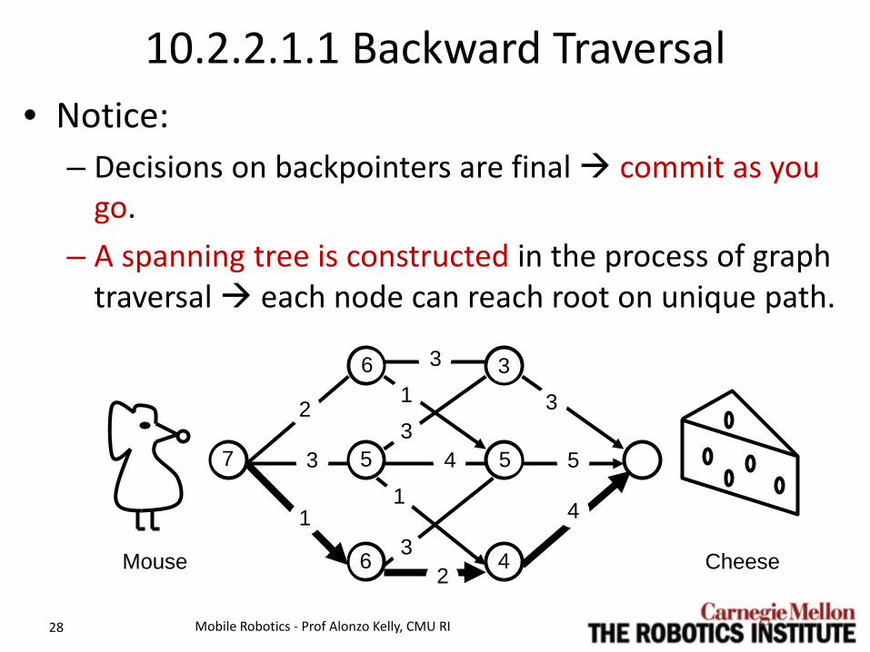
10.2.2.1.1 Backward Traversal • Notice:
– Decisions on backpointers are final commit as you go.
– A spanning tree is constructed in the process of graph traversal each node can reach root on unique path.
Mobile Robotics - Prof Alonzo Kelly, CMU RI 28
Cheese
1
3
2
3
1
1
3
2 3
3
4
4 5
Mouse 4
5
3 6
5
6
7

10.2.2.1.1 Backward Traversal • Notice:
– The nodes or states are a convenient place to store both …
• “best cost so far” • backpointers which record the sequential decisions.
Mobile Robotics - Prof Alonzo Kelly, CMU RI 29
Cheese
1
3
2
3
1
1
3
2 3
3
4
4 5
Mouse 4
5
3 6
5
6
7

Forward Traversal • Branching factor may make one direction preferable. • That will not happen in locally connected graphs like
those derived from grids. • Here, “forward pointers” were remembered to make tree
look the same as last example. Either option is OK for remembering the path.
Mobile Robotics - Prof Alonzo Kelly, CMU RI 30
Cheese
1
3
2
3
1
1
3
2 3
3
4
4 5
Mouse
2
3
1 3
3
5
7
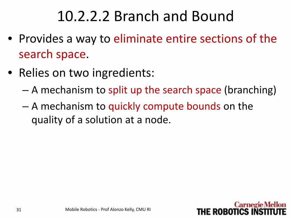
10.2.2.2 Branch and Bound • Provides a way to eliminate entire sections of the
search space. • Relies on two ingredients:
– A mechanism to split up the search space (branching) – A mechanism to quickly compute bounds on the
quality of a solution at a node.
Mobile Robotics - Prof Alonzo Kelly, CMU RI 31
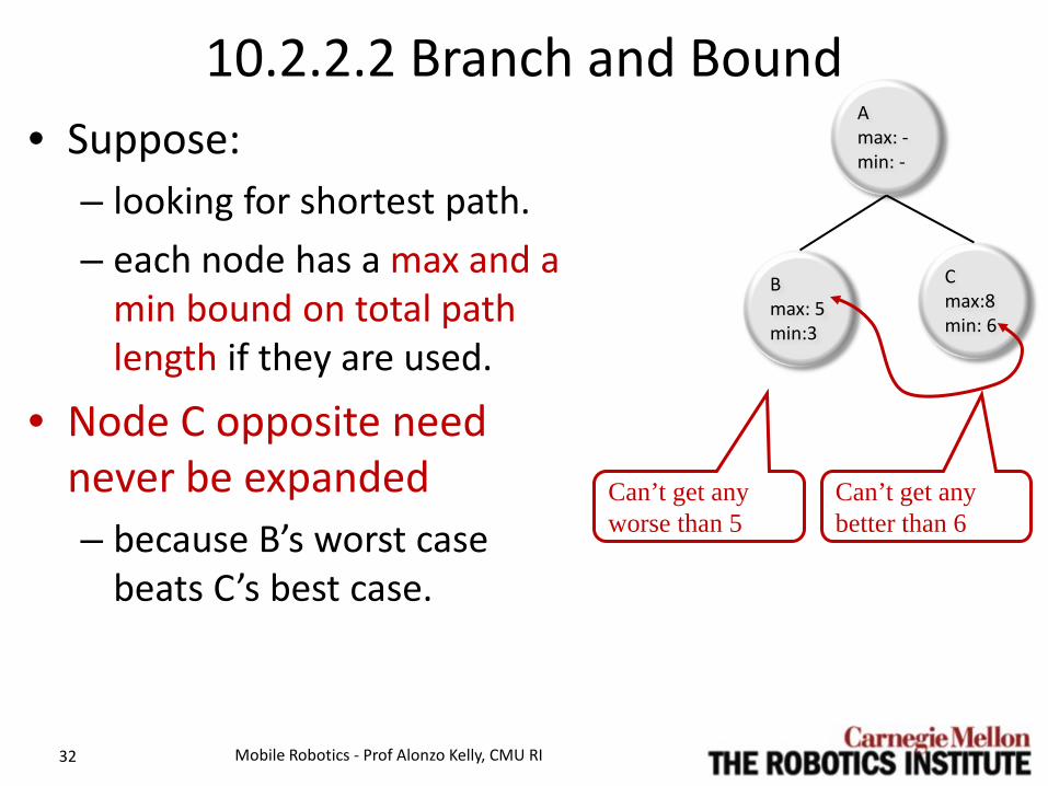
10.2.2.2 Branch and Bound • Suppose:
– looking for shortest path. – each node has a max and a
min bound on total path length if they are used.
• Node C opposite need never be expanded – because B’s worst case
beats C’s best case.
Mobile Robotics - Prof Alonzo Kelly, CMU RI 32
Can’t get any worse than 5
Can’t get any better than 6
A max: - min: -
B max: 5 min:3
C max:8 min: 6
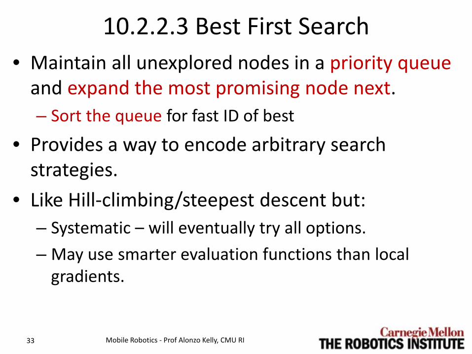
10.2.2.3 Best First Search • Maintain all unexplored nodes in a priority queue
and expand the most promising node next. – Sort the queue for fast ID of best
• Provides a way to encode arbitrary search strategies.
• Like Hill-climbing/steepest descent but: – Systematic – will eventually try all options. – May use smarter evaluation functions than local
gradients.
Mobile Robotics - Prof Alonzo Kelly, CMU RI 33
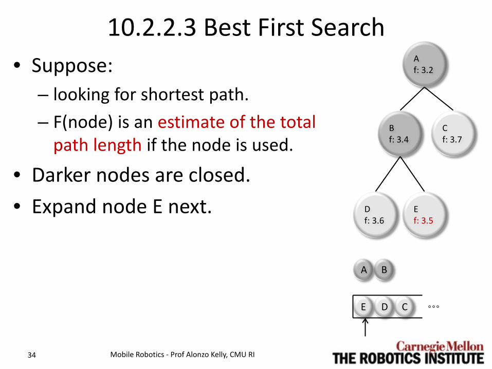
10.2.2.3 Best First Search • Suppose:
– looking for shortest path. – F(node) is an estimate of the total
path length if the node is used.
• Darker nodes are closed. • Expand node E next.
Mobile Robotics - Prof Alonzo Kelly, CMU RI 34
A f: 3.2
B f: 3.4
C f: 3.7
D f: 3.6
E f: 3.5
A B
E D C ˳˳˳
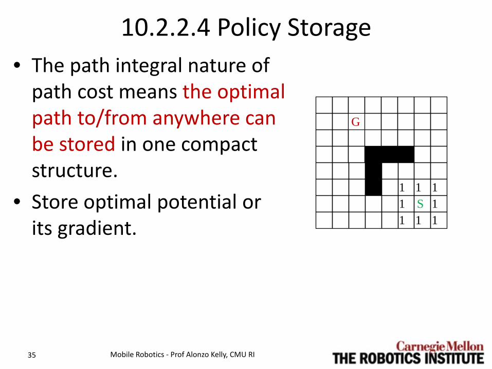
10.2.2.4 Policy Storage • The path integral nature of
path cost means the optimal path to/from anywhere can be stored in one compact structure.
• Store optimal potential or its gradient.
Mobile Robotics - Prof Alonzo Kelly, CMU RI 35
G
1 1 1 1 S 1 1 1 1
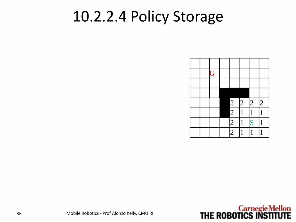
10.2.2.4 Policy Storage
Mobile Robotics - Prof Alonzo Kelly, CMU RI 36
G
2 2 2 2 2 1 1 1 2 1 S 1 2 1 1 1

10.2.2.4 Policy Storage
Mobile Robotics - Prof Alonzo Kelly, CMU RI 37
G
3 3 2 2 2 2 2 1 1 1
3 2 1 S 1 3 2 1 1 1
10.2.2.4 Policy Storage
Mobile Robotics - Prof Alonzo Kelly, CMU RI 38
G 4 4 4
3 3 2 2 2 2
4 2 1 1 1 4 3 2 1 S 1 4 3 2 1 1 1

10.2.2.4 Policy Storage
Mobile Robotics - Prof Alonzo Kelly, CMU RI 39
G 5 5 5 5 5 4 4 4
3 3 5 5 2 2 2 2 5 4 2 1 1 1 5 4 3 2 1 S 1 5 4 3 2 1 1 1

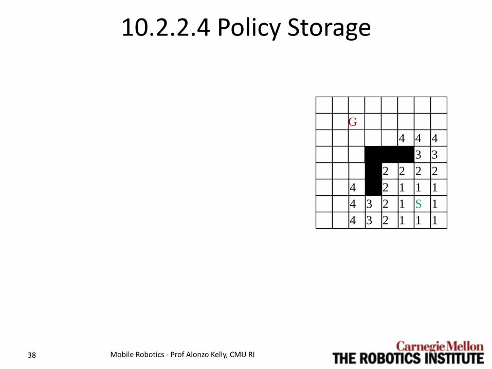
10.2.2.4 Policy Storage • Goal is at distance 7 from
start. • Now know optimal path
from anywhere to the start. – Or from start to anywhere.
Mobile Robotics - Prof Alonzo Kelly, CMU RI 40
8 7 6 6 6 6 6 8 8 7 6 5 5 5 5 7 7 7 5 4 4 4 6 6 6 3 3 6 5 5 2 2 2 2 6 5 4 2 1 1 1 6 5 4 3 2 1 S 1 6 5 4 3 2 1 1 1
6
9

Outline • 10.2 Representation and Search for Global Motion
Planning – 10.2.1 Sequential Motion Planning – 10.2.2 Big Ideas in Optimization and Search – 10.2.3 Uniform Cost Sequential Planning Algorithms – 10.2.4 Weighted Sequential Planning – 10.2.5 Representation For Sequential Motion Planning – Summary
Mobile Robotics - Prof Alonzo Kelly, CMU RI 41
Uniform Cost Edges • Groundrules for the rest of this section… • “Length” of the path is defined as the
number of edges required to reach it. – Edges have equal length or cost.
Mobile Robotics - Prof Alonzo Kelly, CMU RI 42

Reminder: Desiderata • Complete:
– Find a path if it exists – Report failure otherwise (i.e. terminate)
• Sound / Feasible: – Meet all constraints
• Optimal: – Produce optimal solution if any.
Mobile Robotics - Prof Alonzo Kelly, CMU RI 43
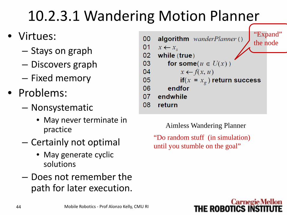
10.2.3.1 Wandering Motion Planner • Virtues:
– Stays on graph – Discovers graph – Fixed memory
• Problems: – Nonsystematic
• May never terminate in practice
– Certainly not optimal • May generate cyclic
solutions – Does not remember the
path for later execution.
Mobile Robotics - Prof Alonzo Kelly, CMU RI 44
Aimless Wandering Planner
“Do random stuff (in simulation) until you stumble on the goal”
“Expand” the node

10.2.3.2 Systematic Motion Planner (Busting Cycles)
• Paths with cycles are better with cycles removed.
• Remember where you’ve been!!
• Side effect: filling up potential “wells”.
• Systematic planners are complete.
• That takes at least some memory. – … e.g. a horizon.
Mobile Robotics - Prof Alonzo Kelly, CMU RI 45
S
G
S
G
S G

10.2.3.2 Systematic Motion Planner (Basics of Search)
• Build a spanning tree of the graph until you hit the goal.
Mobile Robotics - Prof Alonzo Kelly, CMU RI 46
S
1 2
3 5
4
6
7
9 10
G 11
12
8 14
13 15
S G
1
4
3
2
7
5
8
6
9
10
11
12 13
14
15
SEARCH GRAPH Usually elaborated on the fly to save memory
SEARCH TREE Usually encoded in “backpointers”
Wavefront a.k.a. OPEN list
Expanded CLOSED list

10.2.3.2 Systematic Motion Planner • Remembers all visited
states. – Set O is the “open”
(active) frontier. – Set C is the “closed”
(inactive) set.
Mobile Robotics - Prof Alonzo Kelly, CMU RI 47
Move state behind frontier
Terminate on failure
S G

Systematic Planner • Remember parent
pointers to enable path extraction.
• Unique parents creates spanning tree. – = acyclic cover
• Now need memory for O and C.
• Complete. • However, not optimal.
– Unless you sort the O set.
Mobile Robotics - Prof Alonzo Kelly, CMU RI 48
Markers in each state are an efficient alternative to using the set C
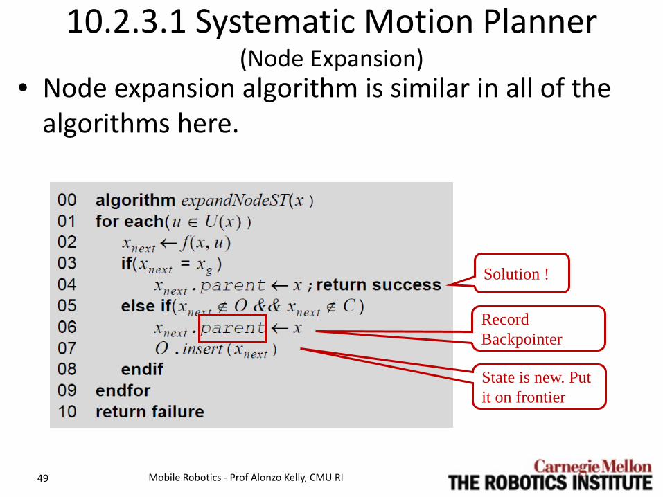
10.2.3.1 Systematic Motion Planner (Node Expansion)
• Node expansion algorithm is similar in all of the algorithms here.
Mobile Robotics - Prof Alonzo Kelly, CMU RI 49
State is new. Put it on frontier
Solution !
Record Backpointer

10.2.3.3 Optimal Motion Planner (BFS / Grassfire)
• Sorted O set. Code looks identical but…
• Set O becomes (ordered) FIFO queue.
• Removed at the front. • Inserted at the back.
Mobile Robotics - Prof Alonzo Kelly, CMU RI 50
Insert at Back

10.2.3.3 Optimal Motion Planner (BFS / Grassfire)
• Called breadth first search on graphs. • Called grassfire on grids. • Generally, the cost of optimality is the sorting.
– But sorting is trivial (FIFO) when edges are uniform cost.
Mobile Robotics - Prof Alonzo Kelly, CMU RI 51
Insert at back
Remove at front
“Wavefront optimality principle” = expand closest node to start.
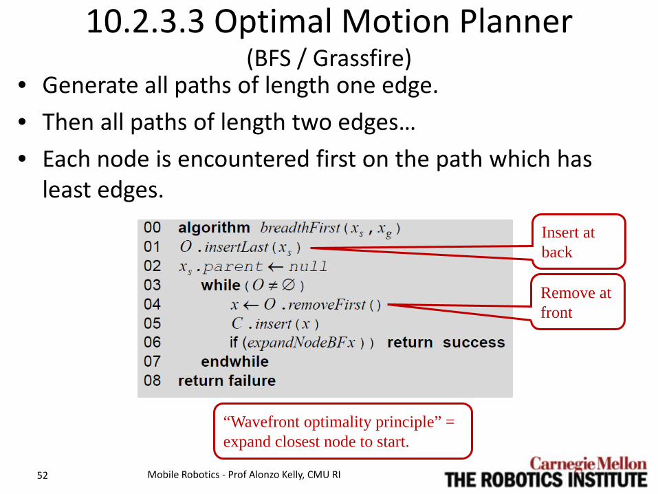
10.2.3.3 Optimal Motion Planner (BFS / Grassfire)
• Generate all paths of length one edge. • Then all paths of length two edges… • Each node is encountered first on the path which has
least edges.
Mobile Robotics - Prof Alonzo Kelly, CMU RI 52
Insert at back
Remove at front
“Wavefront optimality principle” = expand closest node to start.

10.2.3.3 Optimal Motion Planner (BFS / Grassfire)
Mobile Robotics - Prof Alonzo Kelly, CMU RI 53
Wavefront a.k.a. OPEN list
Expanded CLOSED list
World Search Graph (backpointers)
Outline • 10.2 Representation and Search for Global Motion
Planning – 10.2.1 Sequential Motion Planning – 10.2.2 Big Ideas in Optimization and Search – 10.2.3 Uniform Cost Sequential Planning Algorithms – 10.2.4 Weighted Sequential Planning – 10.2.5 Representation For Sequential Motion Planning – Summary
Mobile Robotics - Prof Alonzo Kelly, CMU RI 55

Nonuniform Cost Edges • So far
– ….“length” of the path was defined as the number of edges required to reach it.
• More generally let each edge have a variable, nonnegative cost.
Mobile Robotics - Prof Alonzo Kelly, CMU RI 56
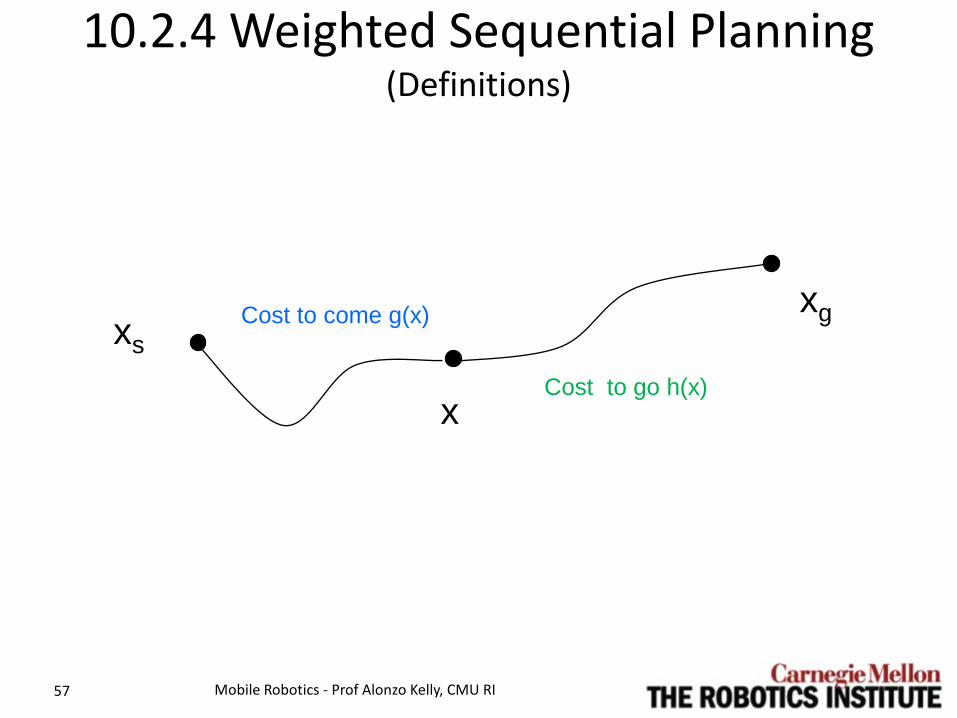
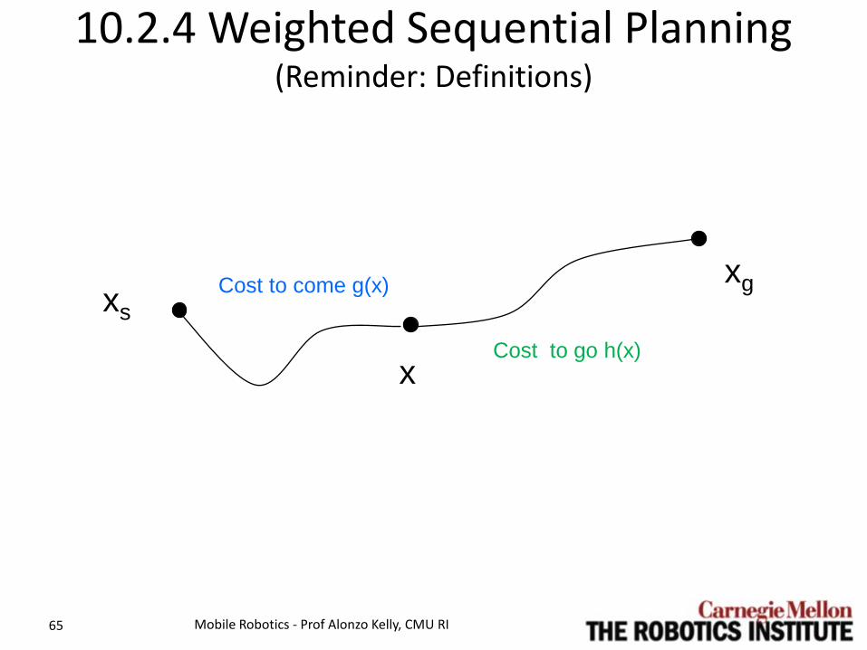
10.2.4 Weighted Sequential Planning (Definitions)
Mobile Robotics - Prof Alonzo Kelly, CMU RI 57
xs xg
x
Cost to come g(x)
Cost to go h(x)

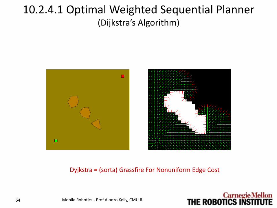
10.2.4.1 Optimal Weighted Sequential Planner (Dijkstra’s Algorithm)
• O becomes a priority queue sorted based on costs-to-come.
• Cost of states expanded increases monotonically – Added states must
exceed cost of parent. – Queue is sorted.
• Invoke wavefront optimality principle.
Mobile Robotics - Prof Alonzo Kelly, CMU RI 58

10.2.4.1 Optimal Weighted Sequential Planner (Dijkstra’s Algorithm)
• New issues: – Cost of nodes added
is no longer monotone.
– Therefore, costs of nodes added may not be optimal.
• So…..
Mobile Robotics - Prof Alonzo Kelly, CMU RI 59
xnext.g
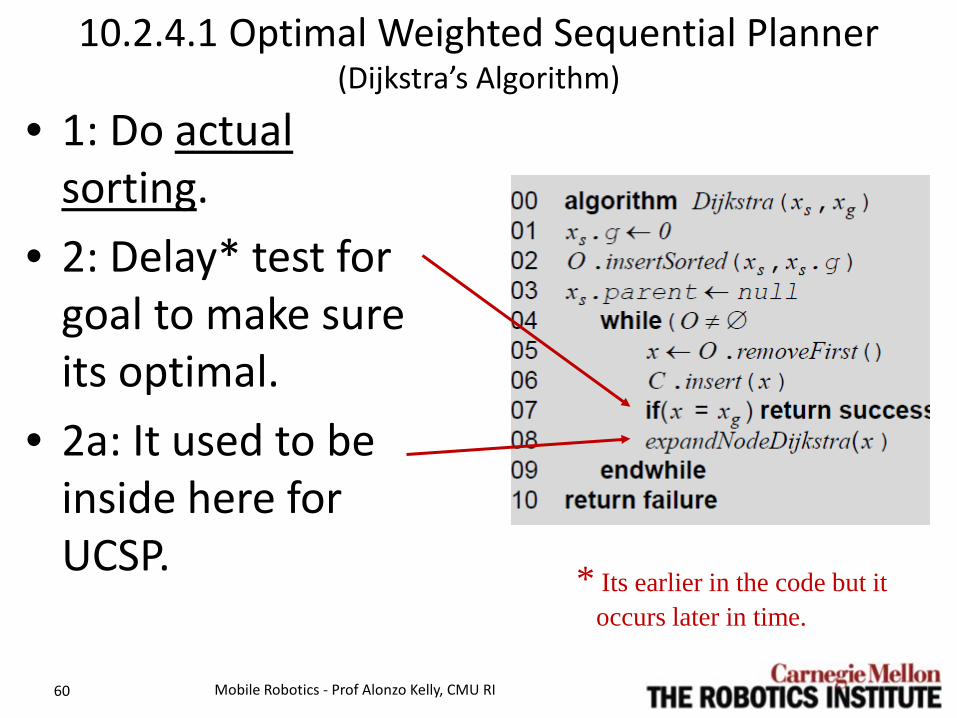
10.2.4.1 Optimal Weighted Sequential Planner (Dijkstra’s Algorithm)
• 1: Do actual sorting.
• 2: Delay* test for goal to make sure its optimal.
• 2a: It used to be inside here for UCSP.
Mobile Robotics - Prof Alonzo Kelly, CMU RI 60
* Its earlier in the code but it occurs later in time.

10.2.4.1 Optimal Weighted Sequential Planner (Dijkstra’s Algorithm)
• 3: permit revisiting nodes – Update costs – Redirect parent
pointers as necessary.
– Remove and reinsert to keep O sorted.
Mobile Robotics - Prof Alonzo Kelly, CMU RI 61
xnext.g
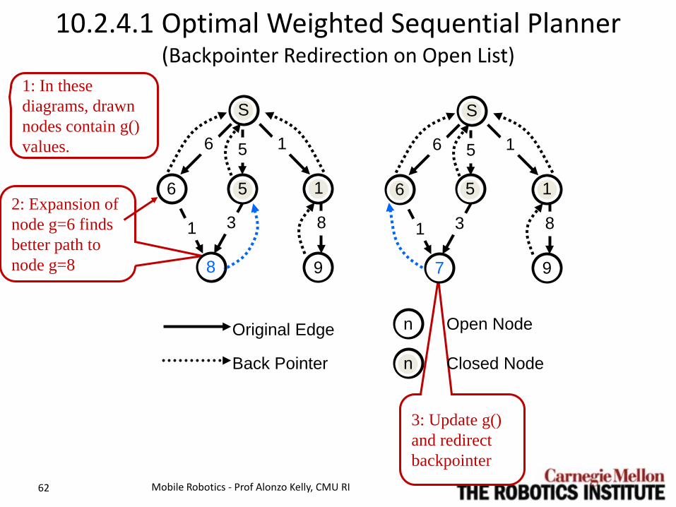
10.2.4.1 Optimal Weighted Sequential Planner (Backpointer Redirection on Open List)
Mobile Robotics - Prof Alonzo Kelly, CMU RI 62
2: Expansion of node g=6 finds better path to node g=8
1: In these diagrams, drawn nodes contain g() values.
3: Update g() and redirect backpointer
S
6 1 5
6 1
8
1 8
9
3
Original Edge
Back Pointer
n Open Node
n Closed Node
S
6 1 5
6 1
7
1 8
9
3
5 5
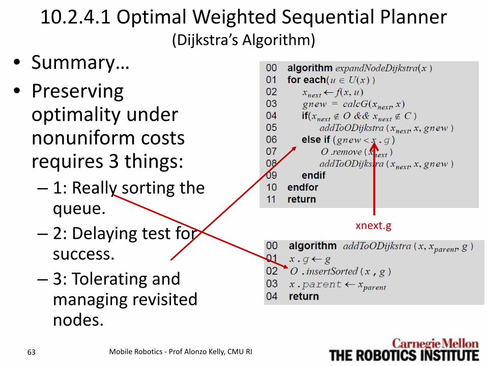
10.2.4.1 Optimal Weighted Sequential Planner (Dijkstra’s Algorithm)
• Summary… • Preserving
optimality under nonuniform costs requires 3 things: – 1: Really sorting the
queue. – 2: Delaying test for
success. – 3: Tolerating and
managing revisited nodes.
Mobile Robotics - Prof Alonzo Kelly, CMU RI 63
xnext.g
10.2.4.1 Optimal Weighted Sequential Planner (Dijkstra’s Algorithm)
Mobile Robotics - Prof Alonzo Kelly, CMU RI 64
Dyjkstra = (sorta) Grassfire For Nonuniform Edge Cost
10.2.4 Weighted Sequential Planning (Reminder: Definitions)
Mobile Robotics - Prof Alonzo Kelly, CMU RI 65
xs xg
x
Cost to come g(x)
Cost to go h(x)

10.2.4.2 Heuristic Optimal Weighted Sequential Planner (A* Algorithm)
• An estimate of the cost-to-go makes it possible to be more efficient and visit less states than Dijkstra’s algorithm
• Now, we store three values in each node, called f() , g() , and h() where: – is the exact known optimal cost-to-come as it is
in Dijkstras algorithm. – is an estimate of the cost-to-go from state to the
goal state. – is an estimate (because its based on ) of the
optimal path cost from the start to the goal through state computed as follows:
Mobile Robotics - Prof Alonzo Kelly, CMU RI 66
g x( )
h x( )
f x( ) h x( )
x
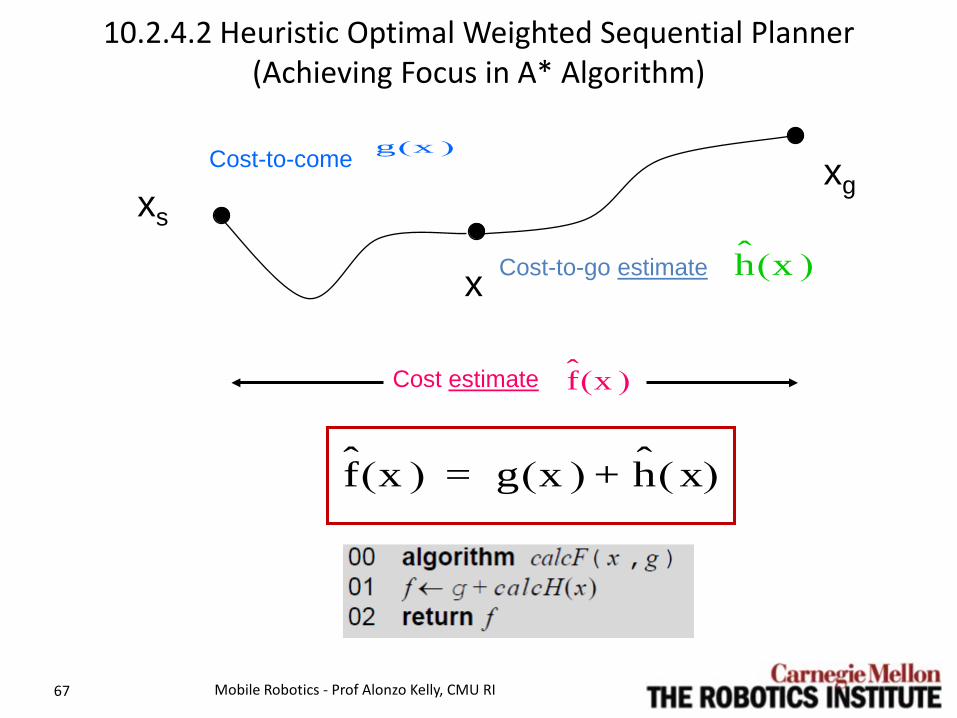
10.2.4.2 Heuristic Optimal Weighted Sequential Planner (Achieving Focus in A* Algorithm)
Mobile Robotics - Prof Alonzo Kelly, CMU RI 67
xs xg
x
Cost-to-come
Cost-to-go estimate
g x( )
h x( )
f x( )Cost estimate
f x( ) g x( ) h x( )+=
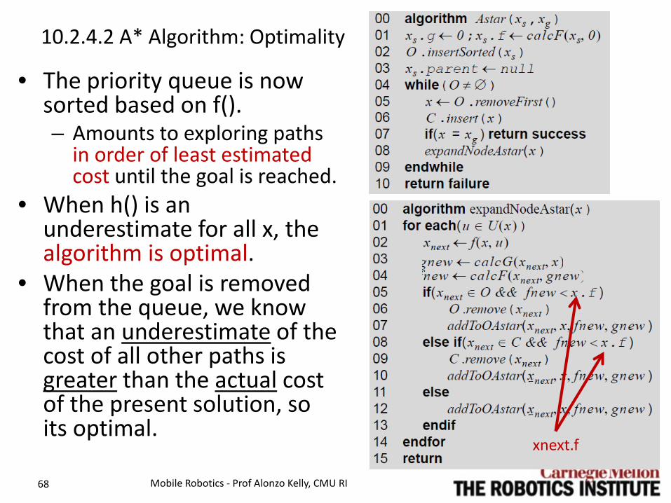
10.2.4.2 A* Algorithm: Optimality
• The priority queue is now sorted based on f(). – Amounts to exploring paths
in order of least estimated cost until the goal is reached.
• When h() is an underestimate for all x, the algorithm is optimal.
• When the goal is removed from the queue, we know that an underestimate of the cost of all other paths is greater than the actual cost of the present solution, so its optimal.
Mobile Robotics - Prof Alonzo Kelly, CMU RI 68
xnext.f
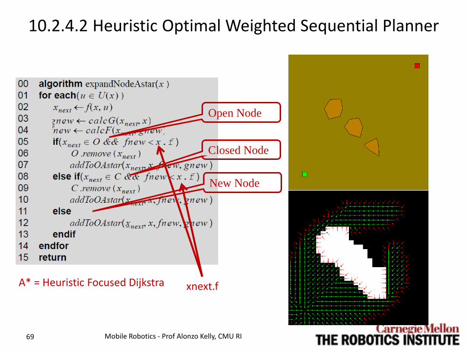
10.2.4.2 Heuristic Optimal Weighted Sequential Planner
Mobile Robotics - Prof Alonzo Kelly, CMU RI 69
Open Node
Closed Node
New Node
A* = Heuristic Focused Dijkstra xnext.f
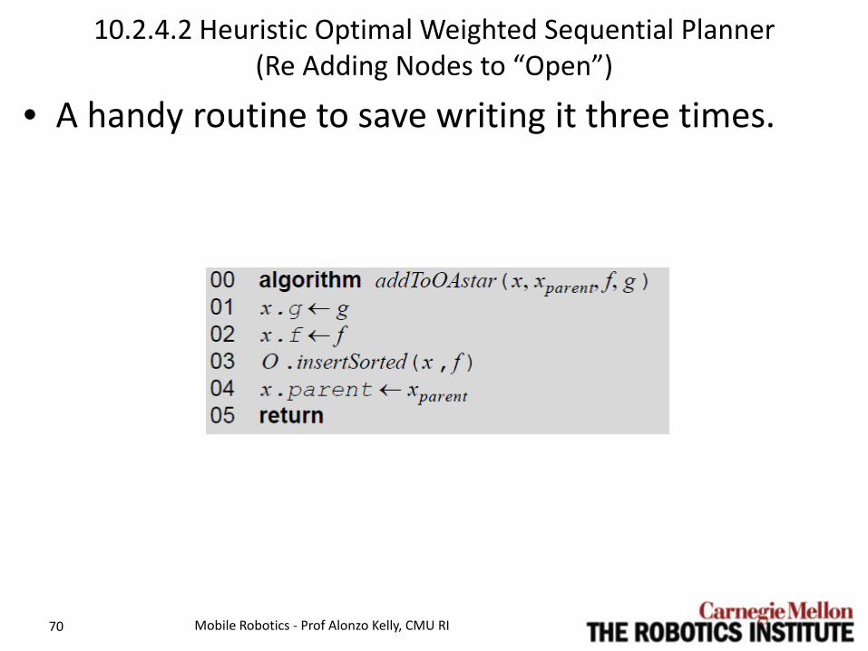
10.2.4.2 Heuristic Optimal Weighted Sequential Planner (Re Adding Nodes to “Open”)
• A handy routine to save writing it three times.
Mobile Robotics - Prof Alonzo Kelly, CMU RI 70

10.2.4.2 Heuristic Optimal Weighted Sequential Planner (A* Facts)
• “Admissability” (implies optimality) – Let h*(x) mean the true optimal cost to the goal from
state x. – h(x) is “admissible” if it is always an underestimate of
the true cost to the goal. • h(x) <= h*(x) always
• Not supposed to call the algorithm A* if h(x) is not admissable. (Call it simply A)
Mobile Robotics - Prof Alonzo Kelly, CMU RI 73

10.2.4.2 Heuristic Optimal Weighted Sequential Planner (A* Facts)
• “Informed” (relates to efficiency) – h1(x) is more informed than h2(x) if:
• h1(x) > h2(x) and … • both are admissable
• A search based on h1(x) will open a subset of the nodes opened using h2(x)
• Hence h1(x) is more efficient.
Mobile Robotics - Prof Alonzo Kelly, CMU RI 74
Its just like the “THE PRICE IS RIGHT!”
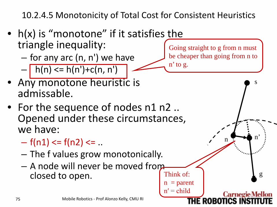
10.2.4.5 Monotonicity of Total Cost for Consistent Heuristics
• h(x) is “monotone” if it satisfies the triangle inequality: – for any arc (n, n') we have – h(n) <= h(n')+c(n, n')
• Any monotone heuristic is admissable.
• For the sequence of nodes n1 n2 .. Opened under these circumstances, we have: – f(n1) <= f(n2) <= .. – The f values grow monotonically. – A node will never be moved from
closed to open.
Mobile Robotics - Prof Alonzo Kelly, CMU RI 75
n n’
g Think of: n = parent n′ = child
s
Going straight to g from n must be cheaper than going from n to n’ to g.

Outline • 10.2 Representation and Search for Global Motion
Planning – 10.2.1 Sequential Motion Planning – 10.2.2 Big Ideas in Optimization and Search – 10.2.3 Uniform Cost Sequential Planning Algorithms – 10.2.4 Weighted Sequential Planning – 10.2.5 Representation For Sequential Motion Planning – Summary
Mobile Robotics - Prof Alonzo Kelly, CMU RI 78
Outline • 10.2 Representation and Search for Global Motion
Planning – 10.2.1 Sequential Motion Planning – 10.2.2 Big Ideas in Optimization and Search – 10.2.3 Uniform Cost Sequential Planning Algorithms – 10.2.4 Weighted Sequential Planning – 10.2.5 Representation For Sequential Motion Planning – Summary
Mobile Robotics - Prof Alonzo Kelly, CMU RI 79

Summary • When vehicles are not omnidirectional, even
planning without obstacles is hard. • Planning in the continuum is not usually
attempted: – when there are significant obstacles or – interesting cost fields. – Instead, convert the problem to an SDP
• For SDPs, techniques of substantial elegance exist. – Sorting a priority queue – Heuristics
Mobile Robotics - Prof Alonzo Kelly, CMU RI 80