Chapter 4

Crop Water Requirement

In this chapter an assessment of crop water requirement in Bhadra command is

made along with the calculations for the scheme water supply for varying cropping

patterns. FAO Water balance computer programme CROPWAT 8.0 model is used.

Meteorological data (temperature, Wind speed, sunshine, relative humidity and rain

fall), crop data (growth dates, crop coefficient and root zone) and soil data (soil

texture, available soil moisture and initial soil moisture) is used to calculate irrigation

water requirements for crops (Allen et al., 1996). In this work, water use for sectors

other than agriculture has not been considered in the water balance, because it is

mostly a non-consumptive use and generally negligible when compared to agriculture

water use.

4.1 Computation of Irrigation Water Requirement

Computation of irrigation water requirements for crops on the basis of the

reference evapotranspiration (ETo) and actual Evapotranspiration (ETa) is made from

the soil-water balance model by using following equation:

IRc (m) =Kc (m) xETo (m)-ETa (m) xAxCI (m) (1)

Where,

IRc Irrigation water requirements to cover crop evapotranspiration Kc Crop coefficient ETo Reference evapotranspiration in mm ETa Actual evapotranspiration A Area under irrigation as percentage of the total area CI Cropping intensity m Monthly time step of the calculation

58

The equation indicates that the crop water requirement is equal to Kc x ETo,

part of which was supplied by the precipitation. When ETa is higher than the water

requirement, the irrigation water requirement is considered nil. CROPWAT model

which adopts the FAO Penman-Monteith method is used to calculate the reference

evapotranspiration (ETo). Relatively accurate and consistent performance of the

Penman-Monteith approach in both arid and humid climates has made this method the

sole standard method for the definition and computation of the reference

evapotranspiration.

4.1.1 Reference Evapotranspiration (ETo)

The evapotranspiration rate from a reference surface, not short of water, is

called the reference crop evapotranspiration or the reference evapotranspiration and is

denoted as ETo. The reference surface is a hypothetical grass reference crop with

specific characteristics. The use of other denominations such as the potential

evapotranspiration is strongly discouraged due to ambiguities in their definitions. The

concept of the reference evapotranspiration was introduced to study the evaporative

demand of the atmosphere independently of the crop type, crop development and

management practices. As water is abundantly available at the reference

evapotranspiration surface, soil factors do not affect evapotranspiration. Relating

evapotranspiration to a specific surface provides a reference to which

evapotranspiration from other surfaces can be related. It obviates the need to define a

separate evapotranspiration level for each crop and stage of growth. ETo values

measured or calculated at different locations or in different seasons are comparable as

they refer to the evapotranspiration from the same reference surface.

59

The need for an accurate and standard method to estimate ETo to predict crop

water requirement has been stated by several authors (Allen et al., 1996; Martmez-

Cob and Tejero-Juste, 2004; Chiew et al., 1995; Allen et al., 2005). A great number of

equations for estimating ETo are reported in literature (Pereira and Pruitt, 2004;

Dehghanisanij et al., 2004; Alexandris et al., 2006; Gavilan et al., 2006;), but, the

International scientific community has accepted the Penman-Monteith equation as the

most precise one for its good results when compared with other equations in various

regions of the entire world (Chiew et al., 1995; Garcia et al., 2004; Gavilan et al.,

2006). Subsequent research has demonstrated the superiority of the Penman-Monteith

equation (Lopez-Urrea et al., 2006; Cai et al., 2007; Cleugh et al., 2007; Xing et al.,

2008; Adeboye et al., 2009 and Liang et al., 2010).

The Penman-Monteith equation is given as.

0.408 A(Rn-G)+Y=?^U2(es-ea)

° A+Y(1+0.34U2) ^ ^

Where,

ETo reference evapotranspiration (mm day'') Rn net radiation at the crop surface (MJ m" day"') G soil heat flux density (MJ m" day'') T mean daily air temperature at 2 m height (°C) U2 wind speed at 2 m height [m s"'] Cs saturation vapour pressure (kPa) Ca actual vapour pressure (kPa) Cs-ea saturation vapour pressure deficit (kPa) A slope vapour pressure curve (kPa °C'') Y psychrometric constant (kPa °C"')

4.1.2 Crop Evapotranspiration (ETc)

Crop evapotranspiration (ETc) refers to the evapotranspiration from the

excellently managed, large, well-watered fields which achieve full production under

the given climatic conditions. ETc is essential for decision making regarding

60

irrigation water management. ETc should be distinguished between crop

evapotranspiration under optimum soil water conditions and under soil water stress,

when the conditions encountered in the field differ from the optimum conditions, a

correction on ETc is required (Allen et al., 2005). Due to the limited water supply and

soil salinity may reduce soil water uptake and limit crop evapotranspiration. The most

popular method of ETc estimation requires the utilization of empirical crop

coefficients. The crop coefficient is used in conjunction with the calculated reference

evapotranspiration to obtain ETo. ETo is a climatic parameter expressing the

evaporation power of the atmosphere.

The calculation of crop evapotranspiration (ETc) consisted of;

1. Identifying the crop growth stages, determining their lengths, and selecting the

corresponding Kc coefficients;

2. Adjusting the selected Kc coefficients for frequency of wetting or climatic

conditions during the stage;

3. Constructing the crop coefficient curve (allowing one to determine Kc values

for any period during the growing period); and

Calculating ETc as the product of ETo and Kc as given in the Equation 3.

ETc = Kc * ETo (3)

lilt 551-l^Z

ETc crop evapotranspiration [mm day"'J yQSDji Kc crop coefficient [dimensionless] ETo reference crop evapotranspiration [mm day]

4.1.2.1 Growth Stages

Growth is the process by which a plant increases in the number and size of

leaves and stems. As the crop develops, the ground cover, crop height and the leaf

.••t-1941 6, KLfvemou Urwerslty Library

.inpr-i Saiivadn Shankaraohatta

area change and differences in evapotranspiration during the various growth stages, in

the study area the paddy is under the duration varieties of 120-147 days including

nursery period, initial stage, development stage and last stage.

According to the analysis and information collected from the field, agriculture

office and farmers, the growth stages identified as the nursery stage about 45 to 50

day and initial stage 20 day, development stage 30 and mid period 40 days then late

stage around 30 days. The NDVl values of paddy in different growth periods and

seasons, show the values between 0.272-0.304 during the initial growth stage. From

26 February to 22 March the NDVI values start increasing, indicating the

development stage. Between 22 March and 2 of May, the NDVI values at its peak

mainly because of the reflectance of greenness of the crop and it indicates that the plot

was in the flowering stage. After this period the NDVI began to the decrease due to

decrease in the greenness of the crops (Fig 4.1).

oso

0.70

0.60

0.30

0.40

0.30

0.20

0.10

0.00

Growth .ftagM 2007

.0.67 0 " n « " « 0.63

0 34 .0.58

0.36 0.40

OJ29 0.29 027"^"

0 56. 0.52

0.46

0.34

A<«<.'Vvv>yv<.>t/>>>>-v • * !

Figure 4.1: Growth Stage of Paddy along with NDVI for the year 2007

4.1.2.2 Crop Coefficient (Kc)

Crop coefficient Kc is the ratio of potential evapotranspiration for a given crop

to the evapotranspiration of a reference crop. The crop coefficient values in Equation

62

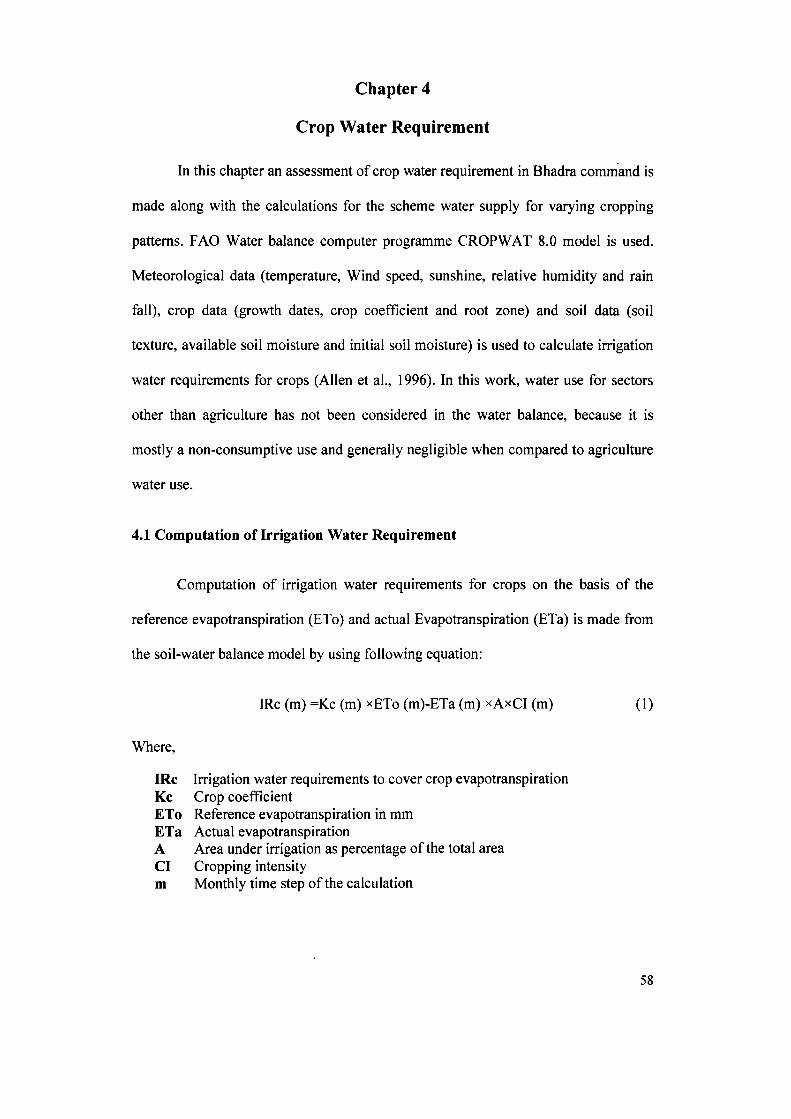
3 are obtained from Allen et al., (1998) for initial, mid and end season according crop

growth stage and separately for each crop. The crop coefficient curve used to

represent coefficient for each crop in particular day or particular time period (Fig 4.2).

Also, the values can be estimated from the standard values by adjusting a number of

factors like temperature, humidity, soil textures and wind speed.

1.20

1.00

2 7 0.80

E 0.60 I 0.40 u

0.20

0

;[y)t

i Initial

>xK \-^ >*i > * f^

- ^ t > ^ - > Crop

dtvelopnwnt i Mid-s«ason Late-season

Time of Season (days or weeks after planling)

Figure 4.2: Crop Coefficient Curve (Allen et al., 1998)

Crop coefficients are relevant and more convenient for normal irrigation

planning and management purposes, for the development of basic irrigation

schedules, and for most hydrologic water balance studies. The crop coefficients for

different crops was developed using the FAO 56 model, three values of crop

coefficients for three important stages of development is determined (Allen et al.,

1998). The crop coefficient for initial stage is referred as Kcmi, similarly crop

coefficients for the mid-season and end stages are designated as Kcmid and Kcend

respectively. Allen et al., (1998) tabulated the values of Kcmi, Kcmid and KCend for

different crops under the standard growing conditions. The mean maximum plant

heights for non-stressed, well-managed crops in sub humid climates (RHmin=45%,

U2~2 m/s). Only three values for Kc was required to adjust and describe the crop

coefficient curve those during the initial stage (Kcjni), the mid-season stage (KCmid)

and at the end of the last season stage (Kcend)-

63

4.1.2.2.1 Determination of Kcini

Evapotranspiration during the initial stage remains predominately in the form

of evaporation. Therefore, the frequency with which the soil surface is wetted during

the initial period is taken into account. The value of Kcini is affected by the

evaporating power of the atmosphere, magnitude of wetting event and the time

interval between wetting events. The Kcini values obtain from Allen et al., (1998), for

example, for paddy the value was found to be 1.10 for arid and semi-arid climate with

calm to moderate wind speeds. The Kcjni should be adjusted for the local climate as

indicated in Allen et al., (1998).

Kci„i-fwKcini(Tab) (4)

Where,

fw the fraction of surface wetted by irrigation or rain ( 0 - 1 ) Kci„i(Tab) the value for Kcini (Allen et al., 1998)

The Kcini can be high where crop ground cover exists, and low when the soil

surface is kept bare and infrequent wetting.

4.1.2.2.2 Crop Coefficient for the Mid-season Stage (Kc mid)

The value of KCmid varies with the climatic conditions and the crop height.

More arid climates and conditions of greater wind speed could have higher values of

Kcmid. Higher humid conditions and lower wind speed would have lower values of

KCmid for specific adjustment in climates U2 is larger or smaller than 2.0 m/s (1 ms' ' <

U2 < 6 ms"') and for RH larger than 20% and smaller than 80% (20% < RHmin < 80%)

(Fig 4.3) then the Kcmid values are adjusted as:

Kc^id = Kc^idCTab) + [0.04(U2 - 2)0.004(RH„i„ - 45)] Q ) ° ' (5)

64

Where,

Kc mid is value for Kcmid taken from (Allen et al., 1998) U2 is the mean value of daily wind speed at 2.0 m height over grass during the

mid- season growth stage (ms"') for 1 ms"' < U2 < 6 ms'' RHmin is mean value of daily minimum relative humidity during the mid-season

growth stage (%) for 80 % (20% < RHmm < 80%) 'h' is The mean plant height during the mid-season stage [m] for 0.1m < h < 10m

Figure 4.3: Adjustment (additive) to the Kc mid values for different crop heights and mean daily wind speeds (U2) for different humid conditions, (Allen et al., 1998)

4.1.2.2.3 Crop Coefficient for the Late Season Stage (Kcend)

The value of Kcend is influenced by crop and water management practices, ff

the crop is irrigated continuously, until harvested, the top layer of soil remains wet

and Kcend value would be relatively high. On the other hand, crops that are allowed to

senesce and dry out in the field before harvest and receive less frequent irrigation or

stop the irrigation during late season stage, consequently both the soil surface and

vegetation are dry and the value for KCgnd will be relatively small. More arid climates

and conditions of greater wind speed would have higher values for Kcend- Higher

humid climates and lower wind speed causes lower values for Kcend- For specific

65

adjustments in climate where U2 is larger or smaller than 2.0 ms"' and relative

humidity differs from the RH larger than 20% or smaller than 80% (20%

<RHmin<80%) then the Kcend will adjust as:

KCend = KCe„d(Tab) + [0.04(U2 - 2)0.004(RH„i„ - 45)] g ) ° ' ' (6)

Where,

Kcend is value of Kcend (Allen, 1998) U2 mean value of daily wind speed at 2 m height over grass during the mid-

season growth stage (ms"') for 1 ms"' < U2< 6 ms"' RHmin mean value of daily minimum relative humidity during the mid-season

growth stage (%) for 20% < RH in < 80 % h mean plant height during the mid-season stage (m) for 0.1 m< h <10 m

4.2 Crop Evapotranspiration under Soil Water Stress conditions (ETa)

Water stress occurs, when the irrigation and precipitation are not sufficient to

supply the full ETc requirement. In these situations, soil water content in the root zone

gets reduced to levels too low to permit plant roots to extract the full ETc amount.

Soil water stress, can have major impacts on plant growth and development.

When it comes to crops, it causes lower yields and possible crop failure. Lower soil

moisture leads to reduced photosynthesis which decreases the growth and

development of plant. Because the Plants absorb water through their roots, the forces

acting on soil water decrease its potential energy and make it less available for the

plant root extraction. When the soil is wet, the water has a high potential energy; it is

relatively free to move and is easily taken up by the plant roots. In dry soils, the water

has a low potential energy and is strongly bound by capillary and absorptive forces to

the soil matrix, and is less easily extracted by the crop and the plants shows symptoms

of stress. The effects of soil water stress on crop ET are described by reducing the

value for the crop coefficient (Allen et al., 1998). This is accomplished by multiplying

66

the crop coefficient with water stress coefficient (Equation 7). In this case the actual

evapotranspiration is less than potential evapotranspiration.

Ks describe the effect of water stress on crop transpiration rather than

evaporation from soil. Where the single crop coefficient is used, the effect of water

stress is incorporated into the Ks as:

ETa=Ks Kc ETo (7)

Where,

ETa is actual crop evapotranspiration [mm/day] Ks is soil water limiting conditions, Ks < 1 for no soil water stress, Ks = 1

4.2.1 Water Stress Coefficient (Ks)

The Water stress coefficient (Ks) allows for describing the effect of soil water

deficit on the crop evapotranspiration, which is assumed to decrease linearly in

proportion to the reduction of water available in the root zone.

Ks value varies from one (no stress) to zero (full stress). Above the upper

threshold of soil water content, water stress is nonexistent and Ks is equal to 1. Below

the lower threshold, the effect is maximum and Ks is 0. Between the thresholds the

shape of the Ks curve determines the magnitude of the effect of soil water stress on

the process (Fig 4.4).

Water content in the root zone can also be expressed by root zone depletion,

Dr, i.e., water shortage relative to the field capacity. At field capacity, the root zone

depletion is zero (Dr = 0). When soil water is extracted by evapotranspiration, the

depletion increases and stress will be induced when Dr becomes equal to Readily

Available Water (RAW). After the root zone depletion exceeds RAW the water

67

content drops below the threshold, the root zone depletion stands high enough to limit

evapotranspiration to less than potential values and the crop evapotranspiration begins

to decrease in proportion to the amount of water remaining in the root zone. Then for

Dr > RAW, Ks is given by:

K. = TAW-Dr TAW-Dr

TAW-RAW ( l -P)TAW (8)

Where,

Ks is a transpiration reduction factor dependent on available soil water (0-1) Dr root zone depletion [mm] TAW total available soil water in the root zone [mm] p fraction of TAW that a crop can extract without suffering water stress [-],

when the root zone depletion is smaller than RAW, Ks = 1 RAW readily available water

The estimation of Ks requires a daily water balance computation for the root

zone, expressed in Equation 12.

I • / t/,r

upper

FC TAW

jliiHVlrVss" - ^ , , J ,

Dr. root 2ono deplelion

PWP

i relative depletion!

I ' ' f"—H 0.0 0.5 1.0

. ! Dr. 1

0.0 P«», TAW P w T A W root zone depletion

Figure 4.4: The Water Stress Coefficient (AquaCrop, FAO, 2010)

68

4.2.1.1 Soil Water Balance

Using the soil water balance equation, one can identify periods of water

stress/excesses which may have adverse effects on the crop performance. This

identification will help in adopting appropriate management practices to alleviate the

constraint and increase the crop yields. Soil water balance account of all quantities of

water added, removed or stored in a given volume of soil during a given period of

time. Then,

Soil water balance = Water Inputs - Losses of water = Change in soil water

Water Inputs = P + Irr + CR (9)

Where,

P is the precipitation Irr is the irrigation CR is the capillary contribution from the ground-water table

The contribution from the ground water would be significant only if the

ground-water table is near the surface.

Water Losses = ET + D + RO (10)

Where,

ET is the evapotranspiration D is the deep drainage further RO is the surface run-off

Then,

Soil water balance = (P + Irr + C) - (ET + D + RO) (II)

If the amount of water in the root zone depletion at the end of day is Dr,i,(n i")

and water content in the root zone at the end of the previous day,i-I(mm), then daily

water balance, expressed in terms of depletion at the end of the day is:

Dr,,= Dr,i.i-(P-RO)i-Irr,-CRi+ETc,i+DPi (12)

69

Where,

Dr,i root zone depletion at the end of day i (mm) Dr, i-i water content in the root zone at the end of the previous day, i-1 (mm) Pi precipitation on day i (mm) ROi runoff from the soil surface on day i (mm) Irri net irrigation depth on day i that infiltrates the soil (mm) CRi capillary rise from the groundwater table on day i (mm) ETc.i crop evapotranspiration on day i (mm) DPi water loss out of the root zone by deep percolation on day i (mm)

If amount of water in the root zone at the beginning is Ml (mm) and at the end

of a given period is M2 (mm), then season water balance, is expressed as:

Or Ml - M2 = P + 1 + CR - ET - D - RO

Ml + P + 1 + CR = ET + D + RO + M2

(13a)

(13b)

4.2.1.2 Total Available Water (TAW)

Total available water (TAW) is the amount of water held between upper limit

water (field capacity, Fc) and lower limit water (permanent wilting point, WP) in the

root zone (Equation 14), and represents the maximum amount of soil water that can

be used by the plants (Fig 4.5).

Figure 4.5: Total Available Water, Soil Water Content in the Root Zone at Field Capacity (Wrpc) and at Permanent Wilting Point (Wrpwp), (AquaCrop, FAO, 2010)

70

The water content above the field capacity cannot be retained in the soil and

will be lost by drainage as deep percolation; likewise, the water content below

permanent wilting point is so strongly attached to the soil matrix that it cannot be

extracted by plant roots. TAW depends on texture, structure and organic matter

content of the soil. It is expressed in mm per meter of soil depth.

Field Capacity (Fc) is the upper limit of water storing in the root zone, held by

the soil against gravity after being saturated and drained, which can be used by crops,

typically attained after one day of rain or irrigation for sandy soils and from two to

three days for heavier-textured soils that contain more silt and clay.

Permanent Wilting Point (PWP) is the lower limit water storing in the root

zone, and remaining in the soil when the plant permanently wilts, it can no longer

extract water. TWA is given as,

TA W = 1 OOOCGFC - Owp) Zr=Wrpc-Wrpwp (14)

Where,

TAW the total available soil water in the root zone [mm] 0FC the water content at field capacity [m^ m" ] Gwp the water content at wilting point [m^ m" ] Zf effective the rooting depth [m] Wrpc soil water content of the root zone at field capacity [mm] Wrpwp soil water content of the root zone at permanent wilting point [mm]

4.2.1.3 Readily Available Water (RAW)

The Readily Available Water (RAW) is the fraction of Total Available Water

(TAW) that a crop can extract from the root zone without suffering water stress.

Although water is theoretically available to the plants up to a water tension equivalent

to the Wilting Point (WP), crop water uptake is reduced well before that point is

reached. When the soil is sufficiently wet, soil water can meet the atmospheric

71

demand of the crop, and water uptake equals the Crop evapotranspiration under

standard conditions (ETc). As the soil water content decreases, water becomes more

strongly bound to the soil matrix and is more difficult to extract. Therefore,

RAW = pTAW (15)

Where,

RAW readily available soil water in the root zone [mm] p average fraction of Total Available Soil Water (TAW) that can be depleted

from the root zone before moisture stress (reduction in ET) occurs.

4.3 Yield-moisture stress relationship

Moisture stress occurs when the water in a plant's cells is reduced to less than

normal levels. This can occur because of a lack of water in the plant's root zone,

higher rates of transpiration than the rate of moisture uptake by the roots; in this case,

plant is unable to absorb water due to high salt content in the soil water or loss of

roots due to transplantation (Allen et al., 1998). Moisture stress is more strongly

related to the water potential than it is to water content. In general, the decrease in

yield due to water deficit during the vegetative and ripening period is relatively small,

while during the flowering and yield formation periods it would be large. A simple,

linear crop-water production function was introduced to predict the reduction in crop

yield Allen et al., (1998) when crop stress was caused by a shortage of soil water as.

Where,

ETa actual evapotranspiration [mm d''] ETc crop evapotranspiration for standard conditions (no water stress) [mm d'"] Ya actual crop yield Ym maximum expected crop yield Ky a yield response factor [-] table

72

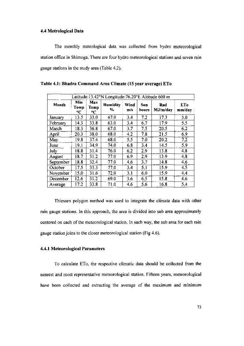
4.4 Metrological Data

The monthly metrological data was collected from hydro meteorological

station office in Shimoga. There are four hydro meteorological stations and seven rain

gauge stations in the study area (Table 4.2).

Table 4.1: Bhadra Command Area Climate (15 year average) ETo

Latitude: 13.42°1 N Longitude:76.20°E AUitude 600 m

Month Min Temp

°C

Max Temp

°C

Humidity %

Wind m/s

Sun hours

Rad MJ/m/day

ETo mm/day

January 13.5 33.0 67.0 3.4 7.2 17.3 5.0 February 14.3 33.8 63.0 3.4 6.7 17.9 5.5 March 18.3 36.8 67.0 3.7 7.5 20.5 6.2 April 20.3 38.0 68.0 4.2 7.8 21.5 6.9 May 19.8 37.4 68.0 5.5 7.0 20.2 7.2 June 19.1 34.9 74.0 6.8 3.4 14.5 5.9 July 18.8 31.4 76.0 6.2 2.9 13.8 4.8 August 18.7 31.2 77.0 6.9 2.9 13.9 4.8 September 18.8 32.4 77.0 4.6 3.7 14.8 4.6 October 17.5 33.3 77.0 3.4 5.1 15.9 4.5 November 15.0 31.6 72.0 3.1 6.0 15.9 4.4 December 12.6 31.2 69.0 3.6 6.5 15.8 4.6 Average 17.2 33.8 71.0 4.6 5.6 16.8 5.4

Thiessen polygon method was used to integrate the climate data with other

rain gauge stations. In this approach, the area is divided into sub area approximately

centered on each of the meteorological station. In such way, the sub area for each rain

gauge station joins to the closer meteorological station (Fig 4.6).

4.4.1 Meteorological Parameters

To calculate ETo, the respective climatic data should be collected from the

nearest and most representative meteorological station. Fifteen years, meteorological

have been collected and extracting the average of the maximum and minimum

73

temperature (°C), relative humidity in percentage, sunsliine hours, average wind run

in m/s to the entire area stations as show in (Table 4.1).

75°28'0"E 75''44'0"E 76°0'0"E

75''28'0"E 75°44'0"E 76°0'0"E

Figure 4.6: Thiessen Polygon Divisions of Meteorological Parameters of Bhadra Right Bank Command Area

74

4.4.1.1 Temperature

Minimum Temperature of the study area in month of December, January,

February, November, Maximum Temperature in month of March, April, May, June

and the average 33.8°C.

4.4.1.2 Humidity

Humidity in the study area varies between a maximum 77% in August,

September and October and a minimum of 63% in February.

4.4.1.3 Wind speed

Wind Speed in the study area is high having the values of 5.5, 6.8, 6.2, 6.9 m/s

in the month of May, June, July and August respectively and medium between 3.7

and 3.1 m/s in the month of March and November respectively.

4.4.1.4 Sunshine hours

Sunshine hours of the study area range between maximum period 7 to 8 hours

in of month January, February, March, April and May the minimum period is 2.9 to

3.7 hours in month of June, July August, September and October. The average

period of sunshine hour is 5.6 hours (Table 4.1).

4.4.1.5 Rainfall data

Calculated daily, decade (ten days) and monthly rainfall available from rain

gauge stations and their spatial variability is shown in Table 4.2.

75

Table 4.2: Monthly Rainfall Data of Rain Gauging Stations from Bhadra Command

Rain gauge stations

Jan Feb Mar Apr May June July Aug Sept Oct Nov Dec Sum

BRP/Lakkavalli 2 1 8 34 69 167 280 232 104 130 38 6 1070 Bhadravathi 0 1 3 33 66 112 168 153 96 118 43 6 800 Anveri 1 0 0 26 31 69 87 93 59 108 33 4 511 Honnali 0 0 6 34 62 97 99 86 105 102 52 7 650 Sasvehalli 0 0 6 34 68 98 124 111 86 152 26 14 720 Basavapatana 0 0 1 32 47 108 124 123 88 113 24 4 665 Channageri 1 2 6 41 63 105 134 144 124 144 46 4 812 Davanagere 0 0 9 27 69 76 87 109 113 83 6 0 580

Harihara 0 0 1 42 37 66 60 72 96 109 1 0 483

Malebennur 0 0 2 46 42 77 73 78 59 102 0 0 479 Santebennur 1 1 2 23 49 112 149 185 145 104 44 3 817

Average 0 1 4 33 54 96 123 124 102 115 26 4 682

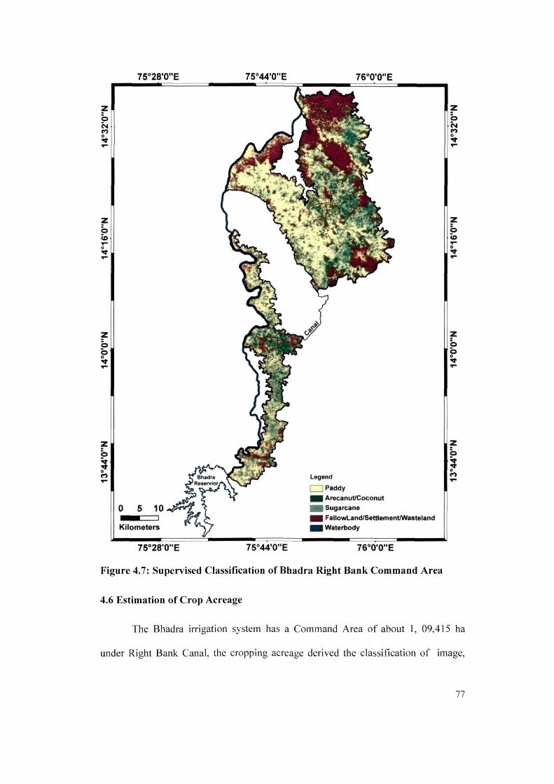
4.5 Supervised Classification

Image classification remains very important to identify feature within the area

of interest. The objective of supervised classification is to categorize every image

pixel into one of several predefined land type classes. In this study, Google Earth and

GPS point (which are taken in the field) are used to categorize the area of interest into

six classes such as paddy, arecanut, coconut, sugar cane, settlement/wasteland/fallow

land, and water body (Table 4.3 and Fig 4.7), with overall accuracy of the

classification is 96.84% see also appendix 4.

Table 4.3: Details of the Classification Images

Classes

Main Branch Canal

Malebennur Branch Canal

Davanagere Branch Canal

Classes Area in

ha Area in

% Area in

ha Area i n %

Area in ha

Area i n %

Paddy 18257.0 48.1 23567.8 64.8 31257.0 37.5 Arecanut 5960.9 15.7 2798.9 7.7 5162.1 6.2 Coconut 4297.1 11.3 2487.0 6.8 6407.3 7.7 Sugarcane 834.0 2.2 363.8 1.0 8022.1 9.6 Fallow land/Wasteland/ Settlement

8488.0 22.4 7086.5 19.5 32114.7 38.5

Water body 116.0 0.3 52.3 0.1 392.2 0.5 Total 37953.0 100.0 36356.0 100 83355.4 100.0

76

75''28'0"E 75O44'0"E 76°0'0"E

o rM

o

Z b b o

z b o CO

1

r^K^^V ^9

Hi ' vs^^^^^SL

^ S ^

r ^ , ^ , - » . . r r

f -i^'**^

t r Bhadra JrReservlorrt

Legend

[ZD Paddy B i Arecanut/Coconut

0 5 1 0 - ^ I B Sugarcane m i FallowLand/Settlement/Wastetand m i Waterbody Kilometers

I B Sugarcane m i FallowLand/Settlement/Wastetand m i Waterbody

o CM CO

I V

O

Z b 5

yS-aS'O-'E 75»44'0"E 76''0'0"E

Figure 4.7: Supervised Classification of Bhadra Right Bank Command Area

4.6 Estimation of Crop Acreage

The Bhadra irrigation system has a Command Area of about 1, 09,415 ha

under Right Bank Canal, the cropping acreage derived the classification of image,

77

found that the paddy covered around 73,082 ha of the total irrigated area, Arecanut

13,922 ha coconut 13,191 ha and Sugarcane 9,220 ha (Table 4.4, 4.5, 4.6 4.10 and

4.11).

Table 4.4: Main Branch Canal Crop Acreage in Hectares

D-No Paddy Areca nut

Coco nut

Total Sugar cane

D-No Paddy Areca nut

Coco nut

Sugar cane

Total

D-1 758 107 104 991 22 D-34 554 155 82 34 825 D-2 786 132 134 1084 32 D-35 183 25 19 3 231 D-3 96 12 16 127 4 D-36 740 102 87 20 951 D-4 141 7 19 177 10 D-37 428 80 59 9 577 D-5 632 82 135 867 18 D-38 208 21 20 1 250 D-6 741 242 259 1271 29 D-39 112 21 35 1 169 D-7 748 112 168 1048 21 D-40 132 25 17 3 177 D-8 739 99 179 1022 5 D-41 102 28 16 2 148 D-9 282 89 94 490 25 D-42 36 8 6 2 52 D-10 283 74 69 440 14 D-43 139 12 21 1 173 D-11 1003 201 303 1555 47 D-44 49 5 5 1 60 D-12 294 48 76 436 17 D-45 968 99 114 47 1228

D-13 442 71 115 658 30 D-46 51 13 12 1 78 D-14 346 189 179 738 24 D-47 392 27 44 4 467 D-15 261 207 113 640 59 D-48 48 16 17 1 82 D-16 236 169 79 520 37 D-49 100 25 26 18 169 D-17 230 164 96 520 29 D-50 76 7 11 1 95 D-18 135 82 65 284 2 D-51 115 6 10 1 132 D-19 212 94 68 383 8 D-52 74 45 22 6 147 D-20 922 225 174 1361 41 D-53 49 23 16 4 94 D-21 566 250 110 942 17 D-54 90 9 7 3 110 D-22 2214 1904 762 4991 HI D-55 7 1 1 0 10 D-23 37 66 16 124 5 D-56 119 29 20 11 179 D-24 162 102 29 305 11 D 57 19 2 1 1 23 D-25 18 4 2 25 0 D 58 16 1 0 1 19 D-26 169 125 64 363 6 D 59 54 9 13 2 78 D-27 23 61 23 109 3 D 60 123 11 8 7 148 D-28 43 38 27 109 1 D 61 40 6 8 1 55 D-29 33 36 17 87 1 D 62 76 9 14 2 101 D-30 31 15 6 53 0 D 63 56 3 7 1 67 D-31 no 59 35 207 2 D 64 60 0 2 1 63 D-32 139 58 30 234 6 D 65 63 2 6 1 72 D-33 42 12 4 60 3 D 66 98 1 3 1 103

Total 18257 5964 4299 834 29354

78

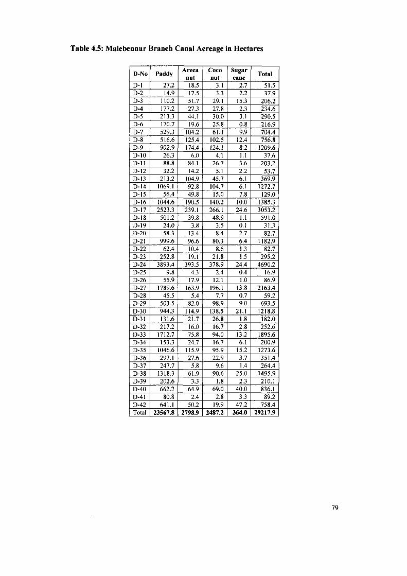
Table 4.5: Malebennur Branch Canal Acreage in Hectares

D-No Paddy Areca

nut Coco nut

Sugar cane

Total

D-1 27.2 18.5 3.1 2.7 51.5 D-2 14.9 17.5 3.3 2.2 37.9 D-3 110.2 51.7 29.1 15.3 206.2 D-4 177.2 27.3 27.8 2.3 234.6 D-5 213.3 44.1 30.0 3.1 290.5 D-6 170.7 19.6 25.8 0.8 216.9 D-7 529.3 104.2 61.1 9.9 704.4 D-8 516.6 125.4 102.5 12.4 756.8 D-9 902.9 174.4 124.1 8.2 1209.6 D-10 26.3 6.0 4.1 1.1 37.6 D-11 88.8 84.1 26.7 3.6 203.2 D-12 32.2 14.2 5.1 2.2 53.7 D-13 213.2 104.9 45.7 6.1 369.9 D-14 1069.1 92.8 104.7 6.1 1272.7 D-15 56.4 49.8 15.0 7.8 129.0 D-16 1044.6 190.5 140.2 10.0 1385.3 D-17 2523.3 239.1 266.1 24.6 3053.2 D-18 501.2 39.8 48.9 1.1 591.0 D-19 24.0 3.8 3.5 0.1 31.3 D-20 58.3 13.4 8.4 2.7 82.7 D-21 999.6 96.6 80.3 6.4 1182.9 D-22 62.4 10.4 8.6 1.3 82.7 D-23 252.8 19.1 21.8 1.5 295.2 D-24 3893.4 393.5 378.9 24.4 4690.2 D-25 9.8 4.3 2.4 0.4 16.9 D-26 55.9 17.9 12.1 1.0 86.9 D-27 1789.6 163.9 196.1 13.8 2163.4 D-28 45.5 5.4 7.7 0.7 59.2 D-29 503.5 82.0 98.9 9.0 693.5 D-30 944.3 114.9 138.5 21.1 1218.8 D-31 131.6 21.7 26.8 1.8 182.0 D-32 217.2 16.0 16.7 2.8 252.6 D-33 1712.7 75.8 94.0 13.2 1895.6 D-34 153.3 24.7 16.7 6.1 200.9 D-35 1046.6 115.9 95.9 15.2 1273.6 D-36 297.1 27.6 22.9 3.7 351.4 D-37 247.7 5.8 9.6 1.4 264.4 D-38 1318.3 61.9 90.6 25.0 1495.9 D-39 202.6 3.3 1.8 2.3 210.1 D-40 662.2 64.9 69.0 40.0 836.1 D-41 80.8 2.4 2.8 3.3 89.2 D-42 641.1 50.2 19.9 47.2 758.4 Total 23567.8 2798.9 2487.2 364.0 29217.9

79

Table 4.6: Davanagere Branch Canal Acreage in Hectares

D-No Paddy Areca

nut Coco nut

Sugar cane

Total

D-1 3964.4 827.6 722.9 409.4 5924.2 D-2 458.6 26.5 55.8 28.8 569.6 D-3 5566.4 938.9 999.6 1251.3 8756.2 D-4 1294.0 174.3 448.5 135.1 2051.9 D-5 142.7 7.5 18.8 9.7 178.7 D-6 461.5 39.0 70.6 42.1 613.1 D-7 967.0 119.5 177.4 108.6 1372.5 D-8 265.2 29.7 60.4 42.7 398.0 D-9 528.2 126.3 157.8 76.8 889.1 D-10 31.5 1.5 6.0 4.8 43.9 D-U 1148.9 219.0 222.9 281.4 1872.3 D-12 436.1 141.9 109.5 197.5 885.0 D-13 50.9 37.1 30.8 60.7 179.5 D-14 1786.9 554.9 640.8 559.0 3541.5 D-15 90.7 7.1 13.3 39.8 150.9 D-16 9210.5 1174.6 1810.6 2473.7 14669.5 D-17 333.1 17.6 61.6 41.8 454.1 D-18 227.0 9.2 17.6 20.2 274.0 D-19 269.7 11.7 29.8 28.7 339.9 D-20 401.9 126.8 93.5 251.2 873.3 D-21 22.2 8.1 5.2 28.5 64.0 D-22 57.1 10.1 8.4 19.4 95.0 D-23 437.4 81.6 86.1 163.8 769.0 D-24 67.5 22.6 16.0 61.0 167.0 D-25 993.5 217.4 173.0 641.5 2025.5 D-26 76.0 16.0 15.6 36.0 143.6 D-27 28.6 1.5 1.0 2.3 33.5 D-28 276.0 17.5 26.2 112.1 431.9 D-29 30.6 3.7 4.0 22.8 61.1 D-30 9.7 1.8 3.2 1.1 15.8 D-31 282.7 13.7 14.3 25.6 336.3 D-32 21.0 2.8 3.2 1.9 29.0 D-33 341.7 47.6 81.3 127.8 598.3 D-34 25.4 0.5 2.7 3.1 31.6 D-35 1.7 0.0 0.0 0.1 1.8 D-36 9.1 0.1 0.5 4.1 13.8 D-37 9.9 0.7 0.6 1.1 12.3 D-38 3.7 0.1 0.9 4.4 9.1 D-39 6.9 1.7 3.4 3.0 15.0 D-40 111.5 21.1 32.4 39.1 204.1 D-41 15.9 0.5 2.8 5.9 25.0 D-42 42.2 9.7 17.8 32.1 101.7 D-43 658.2 76.3 144.2 482.0 1360.6 D-44 23.1 6.6 5.8 29.9 65.4 D-45 8.3 2.7 1.7 7.4 20.1 D-46 0.3 0.2 0.0 0.7 1.3 D-47 0.2 0.0 0.0 0.2 0.4 D-48 5.0 0.0 0.0 1.8 6.8 D-49 35.3 4.8 3.8 33.5 77.3 D-50 0.0 0.0 0.0 0.7 0.7 D-51 0.1 0.0 0.0 5.6 5.7 D-52 13.9 1.1 3.1 13.6 31.7 D-53 0.4 0.1 0.0 5.3 5.8 D-54 4.4 0.9 1.8 34.9 41.9 D-55 1.3 0.0 0.0 5.3 6.5 D-56 1.5 0.0 0.0 1.0 2.5 Total 31257.0 5162.1 6407.0 8022.1 50848.2

80

4.7 Crop Coefficient

Crop coefficient (Kc) estimation is very important in determining the use of

water for selected crop. Reference crop evapotranspiration accounts for the variations

in weather and offers as a measure of the "evaporative demand" of the atmosphere,

crop coefficients accounts as the ratio between the crop evapotranspiration (ETc) and

ETo.

Several methods and models have been adopted to determine crop coefficient

for paddy in different regions of the world with the varying degree of success. Allen

et al., (1998), determined the Kc of paddy and quoted as; 1.5, 1.15 and 0.7 for

vegetative, mid-season and mature stage respectively. Tyagi et al., (2000) found that

the crop coefficient for Kamal, India as 1.15, 1.23, 1.14 and 1.02 for four crop growth

stages on initial, development, reproductive (mid stage) and maturity (late stage),

respectively. Tripaty, (2004) calculated it for Tarai region of Uttaranchal, India as

0.39, 1.0, 1.7, and 0.39 at transplantation, 24 days, 48 days, 66 days and at maturity of

the crop, respectively.

Shah et al., (1986) derived the crop coefficient of paddy at vegetative,

reproductive and maturation stages as 0.96, 1.20, and 1.17 respectively. Tomar and

O'Toole, (1980) found this value as 1.0, 1.15 and 1.3, at transplanting maximum tiller

stage and flowering stage for wetland paddy for central plain of Thailand. Doorenbos

and Kassam, (1979) suggested these values for both wetland and dry season

(December to mid-May) for different geographical locations and seasons. According

to him the values for wet season were 1.10, 1.05, and 0.95 and for dry season are 1.25,

1.10 and 1.0 for first and second month, mid-season and last four weeks respectively,

for humid Asia with light to moderate wind. Murthy and Pillai, (1982) found

81

uniformity coefficient for Arecanut is 0.95 while Mahesha et al., (1990) found

coefficient young Arecanut palms is 0.95-0.99.

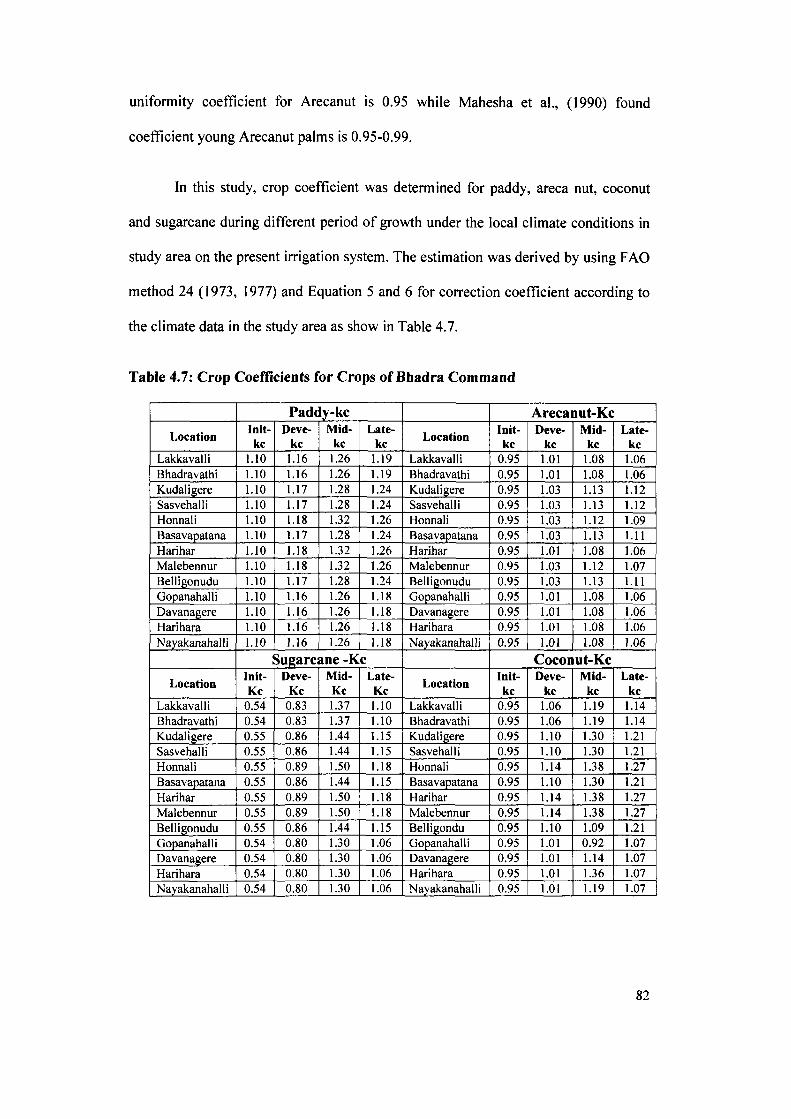
In this study, crop coefficient was determined for paddy, areca nut, coconut

and sugarcane during different period of growth under the local climate conditions in

study area on the present irrigation system. The estimation was derived by using FAO

method 24 (1973, 1977) and Equation 5 and 6 for correction coefficient according to

the climate data in the study area as show in Table 4.7.

Table 4.7: Crop Coefficients for Crops of Bhadra Command

Padd y-kc Arecanut-Kc Location

Init-l(C

Deve-kc

Mid-l(C

Late-kc

Location Init-kc

Deve-kc

Mid-kc

Late-kc

Lakkavalli LIO 1.16 1.26 1.19 Lakkavalli 0.95 1.01 1.08 1.06 Bhadravathi 1.10 1.16 1.26 1.19 Bhadravathi 0.95 1.01 1.08 1.06 Kudaligere 1.10 1.17 1.28 1.24 Kudaligere 0.95 1.03 1.13 1.12 Sasvehalli 1.10 1.17 1.28 1.24 Sasvehalli 0.95 1.03 1.13 1.12 Honnali 1.10 1.18 1.32 1.26 Honnali 0.95 1.03 1.12 1.09 Basavapatana 1.10 1.17 1.28 1.24 Basavapatana 0.95 1.03 1.13 1.11 Harihar 1.10 1.18 1.32 1.26 Harihar 0.95 1.01 1.08 1.06 Malebennur 1.10 1.18 1.32 1.26 Malebennur 0.95 1.03 1.12 1.07 Belligonudu 1.10 1.17 1.28 1.24 Belligonudu 0.95 1.03 1.13 1.11 Gopanahalli 1.10 1.16 1.26 1.18 Gopanahalli 0.95 1.01 1.08 1.06 Davanagere 1.10 1.16 1.26 1.18 Davanagere 0.95 1.01 1.08 1.06 Harihara 1.10 1.16 1.26 1.18 Harihara 0.95 1.01 1.08 1.06 Nayakanahalli 1.10 1.16 1.26 1.18 Nayakanahalli 0.95 1.01 1.08 1.06

Sugarcane -Kc Coconut-Kc Location

Init-Kc

Deve-Kc

Mid-Kc

Late-Kc

Location Init-kc

Deve-kc

Mid-kc

Late-kc

Lakkavalli 0.54 0.83 1.37 1.10 Lakkavalli 0.95 1.06 1.19 1.14 Bhadravathi 0.54 0.83 1.37 1.10 Bhadravathi 0.95 1.06 1.19 1.14 Kudaligere 0.55 0.86 1.44 1.15 Kudaligere 0.95 1.10 1.30 1.21 Sasvehalli 0.55 0.86 1.44 1.15 Sasvehalli 0.95 1.10 1.30 1.21 Honnali 0.55 0.89 1.50 1.18 Honnali 0.95 1.14 1.38 1.27 Basavapatana 0.55 0.86 1.44 1.15 Basavapatana 0.95 1.10 1.30 1.21 Harihar 0.55 0.89 1.50 1.18 Harihar 0.95 1.14 1.38 1.27 Malebennur 0.55 0.89 1.50 1.18 Malebennur 0.95 1.14 1.38 1.27 Belligonudu 0.55 0.86 1.44 1.15 Belligondu 0.95 1.10 1.09 1.21 Gopanahalli 0.54 0.80 1.30 1.06 Gopanahalli 0.95 1.01 0.92 1.07 Davanagere 0.54 0.80 1.30 1.06 Davanagere 0.95 1.01 1.14 1.07 Harihara 0.54 0.80 1.30 1.06 Harihara 0.95 1.01 1.36 1.07 Nayakanahalli 0.54 0.80 1.30 1.06 Nayakanahalli 0.95 1.01 1.19 1.07

82

4. 8 Soil Data

The soil of the study area is a mixture of sand, gravel and clay. The surface

texture varies from clay, clay loam, gravelly loam, loam, sandy loam, sandy clay, and

sandy clay loam. The major part of the area is covered by sandy loam, sandy clay, and

sandy clay loam (Fig 3.7). This information is obtained from Kamataka soil map and

manipulated by Texture Auto Lookup (TAL 4.2). TAL determines the soil texture

class based on USDA (Christopher and Mokhtaruddin, 1996).

Information from the soil surveys carried out in the Bhadra Command Area

shows two distinct soil categories:

• Red sandy loams, red loamy and red sandy, covering 23% of the

Command Area, relatively shallow and free-draining, particularly suitable

for upland crops.

• Black clay soils, covering 77%, deep but poorly drained, suitable mainly

for paddy and deep rooting crops like cotton.

4.8.1 Soil Water Characteristics

Soil-Water potential and hydraulic conductivity relationship with soil-water

content are needed for many plants and soil-water studies. Hydrologic analyses often

involve the evaluation of soil water infiltration, conductivity, storage, and plant-water

relationships. To define the hydrologic soil water effects, requires an estimation of

soil water characteristics for water potential and hydraulic conductivity using soil

variables such as texture, organic matter and structure.

An approximate measurement of soil-water was done through the use of the

soil texture triangle and the pedotransfer functions. A simple hydraulic properties

calculator for this purpose is available in the Internet at:

83

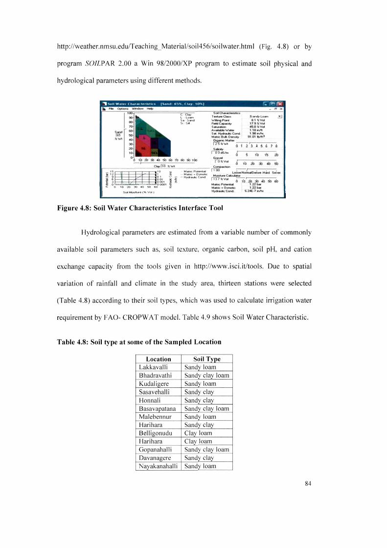
http://weather.nmsu.edu/Teaching_Material/soil456/soilwater.html (Fig. 4.8) or by

program SOILPAR 2.00 a Win 98/2000/XP program to estimate soil physical and

hydrological parameters using different methods.

IS5

1. -Lo«n S* Sand S. S*

WiteigPo«il T«Mh«* ClM« |S«nt^ Lown

e i KVol 179XVOI 4 5 0 * Vol

Av^ifclfl W « f 1 18n/n $«( Hy<ft«L*C Cond 1 96 v^/h M«1M: BtA D«nt«y 91 01 b.^3 Oig.

0 i o 2 0 » « ) » e o 7 a a o 9 0 i t e — ] roxvoi

A 1 i i 4 i i » i

r^ Vo ih i )

A 10 A 3b 4) A

S'i

O 10 » » 40 %0 so

Sod Motst<jre (X vol)

01 0 01 OOOl 0 0OO1 ^

ii M«tn; Pol«n(i«l Matnc • OMnotK

- Hy(*«L*c Cond

" (Too LooMMoniMfOonM H«d Sv

( t3 7XVo* 6 10 A 3>] «0 «b

Mottic Polonhil 1 22 boi Maine • Otfnotac 122b«i

Figure 4.8: Soil Water Characteristics Interface Tool

Hydrological parameters are estimated from a variable number of commonly

available soil parameters such as, soil texture, organic carbon, soil pH, and cation

exchange capacity from the tools given in http://www.isci.it/tools. Due to spatial

variation of rainfall and climate in the study area, thirteen stations were selected

(Table 4.8) according to their soil types, which was used to calculate irrigation water

requirement by FAO- CROPWAT model. Table 4.9 shows Soil Water Characteristic.

Table 4.8: Soil type at some of the Sampled Location

Location Soil Type Lakkavalli Sandy loam Bhadravathi Sandy clay loam Kudaligere Sandy loam Sasavehalii Sandy clay Honnali Sandy clay Basavapatana Sandy clay loam Maiebennur Sandy loam Harihara Sandy clay Belligonudu Clay loam Harihara Clay loam Gopanahalli Sandy clay loam Davanagere Sandy clay Nayakanahalli Sandy loam

84

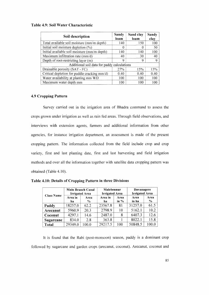
Table 4.9: Soil Water Characteristic

Soil description Sandy loam

Sand clay loam

Sandy clay

Total available soil moisture (mm/m depth) 140 150 100 Initial soil moisture depletion (%) 0 0 50 Initial available soil moisture (mm/m depth) 140 140 100 Maximum infiltration rate (mm/d) 40 30 40 Depth of root-restricting layer (m) 9 9 9

Additional soil data for paddy calculations Drainable porosity (SAT - FC) 27% 15% 15% Critical depletion for puddle cracking mm/d) 0.40 0.40 0.40 Water availability at planting mm WD 100 100 100 Maximum water depth mm 100 100 100

4.9 Cropping Pattern

Survey carried out in the irrigation area of Bhadra command to assess the

crops grown under irrigation as well as rain fed areas. Through field observations, and

interviews with extension agents, farmers and additional information from other

agencies, for instance irrigation department, an assessment is made of the present

cropping pattern. The information collected from the field include crop and crop

variety, first and last planting date, first and last harvesting and field irrigation

methods and over all the information together with satellite data cropping pattern was

obtained (Table 4.10).

Table 4.10: Details of Cropping Pattern in three Divisions

Class Name

Main Branch Canal Irrigated Area

Malebennur Irrigated Area

Davanagere Irrigated Area

Class Name Area in

ha Area

% Area in

ha Area in%

Area in ha

Area %

Paddy 18257.0 62.2 23567.8 81 31257.0 61.5

Arecanut 5960.9 20.3 2798.9 10 5162.1 10.2

Coconut 4297.1 14.6 2487.0 8 6407.3 12.6

Sugarcane 834.0 2.8 363.8 1 8022.1 15.8

Total 29349.0 100.0 29217.5 100 50848.5 100.0

It is found that the Rabi (post-monsoon) season, paddy is a dominant crop

followed by sugarcane and garden crops (arecanut, coconut). Arecanut, coconut and

85

sugarcane formed 33% of the irrigated area and 67% of the paddy (Table 4.11). Paddy

transplantation starts from 25 January to middle of March and the harvesting date

starts from 15 may to 15 of June.

Table 4.11: Total Irrigate/Cropped Area of the Bhadra command

Class Name

Total Irrigated area in ha

Area %

Paddy 73082 67 Arecanut 13922 13 Coconut 13191 12 Sugarcane 9220 8 Total 109415 100

4.10 Calculation Crop Water Requirement in the Main Branch Canal

The Climate data is the primary data input, along with the information on the

meteorological station (country, name, altitude, latitude and longitude) that can be

inputted on a monthly, decade or daily basis. CROPWAT requires climatic

parameters of temperature, humidity, wind speed and sunshine. Regarding to Bhadra

command the spatial distributions of the stations provide a network of the typical

climatic gradients in terms of different latitudes and longitudes covering a wide range

of climatic regions. All selected weather stations have good quality daily data records

from 1984 to 2010 for estimating ETo with the FAO Penman-Monteith method. The

method was applied to all the observed data sets to assess the time length of the data

series required to get reasonably good estimations as is described for three stations in

Table 4.12, 4.13 and 4.14, for other stations data is available in Appendix 2.

86

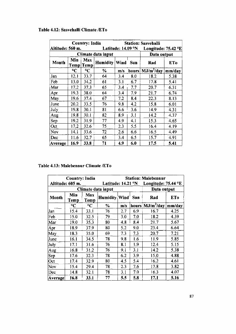
Table 4.12: Sasvehalli Climate /ETo

Country: India Station: Sasvehalli Altitude: 560 m. Latitude: 14.09 °N Longitude: 75.42 ''E

C imate data input Data output

Month Min Temp

Max Temp Humidity Wind Sun Rad ETo

°C °C % m/s hours MJ/m /day mm/day Jan 12.1 33.7 64 3.4 8.0 18.2 5.38 Feb 13.0 34.2 61 3.1 6.7 17.8 5.41 Mar 17.2 37.3 65 3.4 7.7 20.7 6.31 Apr 19.3 38.0 64 3.4 7.9 21.7 6.74 May 19.6 37.4 67 7.2 8.4 22.3 8.13 June 20.2 33.5 76 9.8 4.2 15.8 6.01 July 19.8 30.1 81 6.6 3.6 14.9 4.31 Aug 19.8 30.1 82 8.9 3.1 14.2 4.37 Sep 19.2 31.9 77 4.9 4.1 15.3 4.65 Oct 17.2 32.6 75 2.3 5.5 16.4 4.19 Nov 14.1 33.6 72 2.6 6.6 16.5 4.49 Dec 11.6 32.7 65 3.4 6.5 15.7 4.91 Average 16.9 33.8 71 4.9 6.0 17.5 5.41

Table 4.13: Malebennur Climate /ETo

Country: India Station: Malebennur Altitude: 605 m. Latitude: 14.21 °N Longitude: 75.44 °E

Climate data input Data output

Month Min Temp

Max Temp Humidity Wind Sun Rad ETo

°C °C % m/s hours MJ/mVday mm/day Jan 15.4 33.1 76 2.7 6.9 16.7 4.25 Feb 15.0 32.5 79 3.0 7.0 18.2 4.39 Mar 19.0 35.3 80 4.8 8.4 21.7 5.67 Apr 18.9 37.9 80 5.2 9.0 23.4 6.64 May 18.3 35.0 69 7.3 7.3 20.7 7.21 June 16.1 34.5 78 9.8 1.6 11.9 5.85 July 17.1 31.6 76 8.1 1.9 12.4 5.15 Aug 16.8 31.2 76 9.1 3.1 14.2 5.38 Sep 17.6 32.3 78 6.2 3.9 15.0 4.88 Oct 17.4 32.9 80 4.5 5.4 16.2 4.61 Nov 15.4 29.4 78 2.3 7.6 17.8 3.82 Dec 14.8 32.1 78 3.1 7.0 16.3 4.07 Average 16.8 33.1 77 5.5 5.8 17.1 5.16

87

Table 4.14: Davanagere Climate /ETo

Country: India Station: Davanagere Altitude: 602 m. Latitude: 14.27 °N Longitude: 75.55 °E

Climate data input Data output

Month Min

Temp Max

Temp Humidity Wind Sun Rad ETo

°C °C % m/s hours MJ/mVday mm/day Jan 13.6 34.0 60 2.4 6.1 15.6 4.6 Feb 14.0 34.3 55 2.7 5.0 15.3 5.16 Mar 18.3 37.4 59 2.7 6.4 18.7 5.86 Apr 20.3 38.0 62 3.1 5.7 18.3 6.16

May 20.1 37.6 66 3.2 4.7 16.7 5.79

June 20.1 36.0 70 3.2 3.3 14.5 5.01 July 19.8 32.8 78 3.3 2.5 13.3 4.07

Aug 19.5 32.1 80 2.5 2.5 13.3 3.61 Sep 19.2 34.2 78 1.9 2.4 12.8 3.58

Oct 18.6 35.4 80 2.5 3.4 13.3 3.96

Nov 15.1 32.0 69 2.1 5.1 14.5 4.0

Dec 11.5 29.6 63 2.4 7.0 16.3 4.11

Average 17.5 34.5 68 2.7 4.5 15.2 4.66

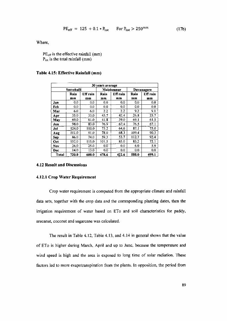
4.11 Effective Rainfall

Defined as that part of the rainfall, which is effectively used by the crop after

rainfall losses due to surface run off and deep percolation have been accounted for.

The effective rainfall is the rainfall ultimately used to determine the crop irrigation

requirements. So to calculate effect rainfall the monthly average of 30 years rainfall

data of each station in the study area is fed into the CROPWAT model from the Table

4.2 and the output result is show in Table 4.15.

There are four common empirical methods for calculating effective rainfalls

(Smith et al., 1991) as follows: (1) fixed percentage of rainfall (2) dependable rainfall

(3) empirical formula and (4) United States Department of Agriculture (USDA) Soil

Conservation Service Method. The USDA Soil Conservation Service Method was

used in this study. The empirical equations are briefed as follows:

PEeff = Ptot * Hlzgftot For P,ot < 2 5 0 - - (17a)

88

PEpff = 125 + 0.1 * P, tot For Pt„t > ZSC (17b)

Where,

PEeff is the effective rainfall (mm) Ptot is the total rainfall (mm)

Table 4.15: Effective Rainfall (mm)

30 years average Sasvehalli Maiebennur Davanagere

Rain mm

EfT rain mm

Rain mm

EfT rain mm

Rain mm

EfT rain mm

Jan 0.0 0.0 0.0 0.0 0.0 0.0 Feb 0.0 0.0 0.0 0.0 0.0 0.0 Mar 6.0 6.0 2.2 2.2 9.2 9.1 Apr 35.0 33.0 45.7 42.4 26.8 25.7 May 69.0 61.0 41.8 39.0 69.1 61.5 Jun 98.0 83.0 76.9 67.4 76.5 67.1 Jul 124.0 100.0 73.2 64.6 87.1 75.0 Aug 111.0 91.0 78.0 68.3 109.4 90.3 Sep 86.0 74.0 59.3 53.7 112.7 92.4 Oct 152.0 115.0 101.5 85.0 83.2 72.1 Nov 26.0 25.0 0.0 0.0 6.0 5.9 Dec 14.0 13.0 0.0 0.0 0.0 0.0

Total 720.0 600.0 478.6 422.6 580.0 499.1

4.12 Result and Discussions

4.12.1 Crop Water Requirement

Crop water requirement is computed from the appropriate climate and rainfall

data sets, together with the crop data and the corresponding planting dates, then the

irrigation requirement of water based on ETo and soil characteristics for paddy,

arecanut, coconut and sugarcane was calculated.

The result in Table 4.12, Table 4.13, and 4.14 in general shows that the value

of ETo is higher during March, April and up to June, because the temperature and

wind speed is high and the area is exposed to long time of solar radiation. These

factors led to more evapotranspiration from the plants. In opposition, the period from

89

July to December where the area is exposes to low radiation and temperature and also

wind speed is moderate and therefore, the ETo is low.

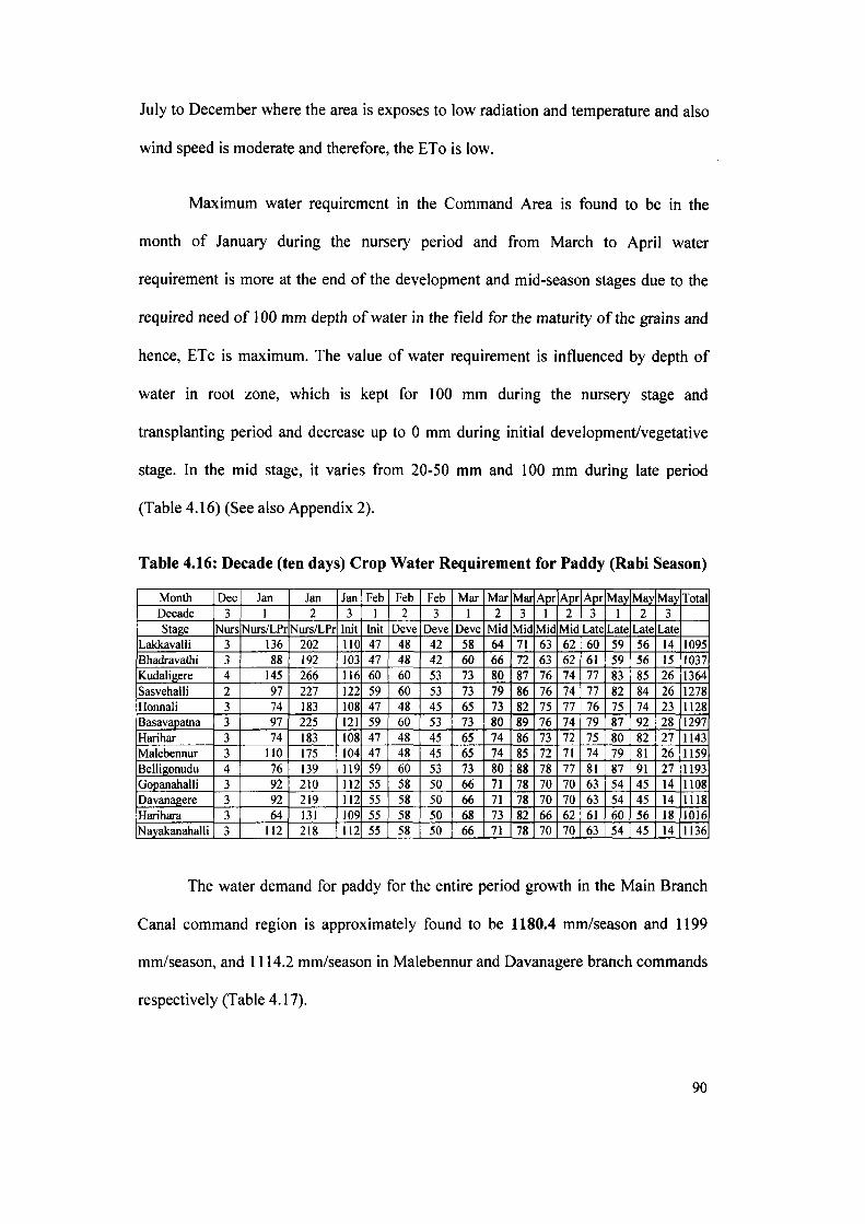
Maximum water requirement in the Command Area is found to be in the

month of January during the nursery period and from March to April water

requirement is more at the end of the development and mid-season stages due to the

required need of 100 mm depth of water in the field for the maturity of the grains and

hence, ETc is maximum. The value of water requirement is influenced by depth of

water in root zone, which is kept for 100 mm during the nursery stage and

transplanting period and decrease up to 0 mm during initial development/vegetative

stage. In the mid stage, it varies from 20-50 mm and 100 mm during late period

(Table 4.16) (See also Appendix 2).

Table 4.16: Decade (ten days) Crop Water Requirement for Paddy (Rabi Season)

Month Dec Jan Jan Jan Feb Feb Feb Mar Mar Mar Apr Apr Apr May May May Total Decade 3 1 2 3 1 2 3 1 2 3 1 2 3 1 2 3 Stage Nurs Nurs/LPr Nurs/LPr Init Init Deve Deve Deve Mid Mid Mid Mid Late Late Late Late

Lakkavalli 3 136 202 110 47 48 42 58 64 71 63 62 60 59 56 14 1095 Bhadravathi 3 88 192 103 47 48 42 60 66 72 63 62 61 59 56 15 1037 Kudaligere 4 145 266 116 60 60 53 73 80 87 76 74 77 83 85 26 1364 Sasvehalli 2 97 227 122 59 60 53 73 79 86 76 74 77 82 84 26 1278 Honnali 3 74 183 108 47 48 45 65 73 82 75 77 76 75 74 23 1128 Basavapatna 3 97 225 121 59 60 53 73 80 89 76 74 79 87 92 28 1297 Harihar 3 74 183 108 47 48 45 65 74 86 73 72 75 80 82 27 1143 Malebennur 3 110 175 104 47 48 45 65 74 85 72 71 74 79 81 26 1159 Belligonudu 4 76 139 119 59 60 53 73 80 88 78 77 81 87 91 27 1193 Gopanahalli 3 92 210 112 55 58 50 66 71 78 70 70 63 54 45 14 1108 Davanagere 3 92 219 112 55 58 50 66 71 78 70 70 63 54 45 14 1118 Harihara 3 64 131 109 55 58 50 68 73 82 66 62 61 60 56 18 1016 Nayakanahalli 3 112 218 112 55 58 50 66 71 78 70 70 63 54 45 14 1136

The water demand for paddy for the entire period growth in the Main Branch

Canal command region is approximately found to be 1180.4 mm/season and 1199

mm/season, and 1114.2 mm/season in Malebennur and Davanagere branch commands

respectively (Table 4.17).

90

Table 4.17: Monthly Average Water Requirements for Paddy in the Bhadra Command

Main Branch Canal Location Dec Jan Feb Mar Apr May Total Bhadravathi 3 448 137 193 186 129 1095 Honnali 2 447 173 238 226 191 1227 Kudaligere 4 527 173 241 227 193 1364 Laldcavalli 3 384 137 197 187 130 1037 Sasvehalli 3 365 140 220 228 172 1178

Total 15 2171 760 1089 1054 815 1180.4' Malebennur Branch Canal

Basavapatana 3 442 173 243 228 207 1297 Harihar 3 365 140 225 221 189 1143 Malebennur 3 389 140 224 218 186 1159

Total 9 1197 453 692 666 581 1199" Davanagere Branch Canal

Belligonudu 3.6 333.5 172.5 241.4 236.4 205.1 1192.5 Davanagere 3.1 422.7 162.2 214.6 203.2 112.1 1117.9 Gopanahalli 3.1 413.0 162.2 214.7 203.2 112.1 1108.3 Harihara 3.1 303.6 162.2 223.0 189.6 134.0 1015.5 Nayokanahalli 3.1 441.3 162.2 214.7 203.2 112.1 1136.6

Total 16.0 1914.1 821.3 1108.4 1035.6 675.4 1114.2* * Average water requirement for respective command 1159.5*

The annual corps like arecanut, coconut and sugarcane the total water

requirement was found to be 1267.62 mm/year, 1564.22 mm/year and 1582.03

mm/year respectively (Table 4.18).

Table 4.18: The Irrigation Water Requirement in mm for Annual Crops

Location Main Branch Canal

Location Arecanut Coconut Sugarcane

Bhadravathi 1014.7 1228.5 1274.3 Honnali 1347.0 1838.3 1830.0 Kudaligere 1370.9 1724.5 1708.1 Lakkavalli 936.2 1122.7 1166.9 Sasvehalli 1413.9 1771.3 1754.4 Average 1216.54 1537.06 1546.74

Malebennur Branch Canal Basavapatana 1453.20 1811.00 1795.50 Harihar 1265.50 1974.00 1966.20 Malebennur 1482.50 1974.90 1966.60 Average 1400.40 1919.97 1909.43

Davana gere Branch Canal Belligonudu 1362.8 1721.0 1706.0 Davanagere 1188.9 1273.0 1330.4 Gopanahalli 1189.5 1273.5 1330.8 Harihara 1264.7 1348.8 1406.4 Nayakanahalli 1189.3 1273.4 1330.8 Average 1239.0 1377.9 1420.9 All stations Average 1267.62 1564.22 1582.03

91

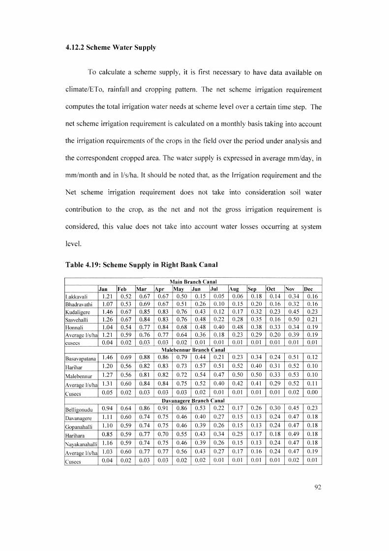
4.12.2 Scheme Water Supply

To calculate a scheme supply, it is first necessary to have data available on

climate/ETo, rainfall and cropping pattern. The net scheme irrigation requirement

computes the total irrigation water needs at scheme level over a certain time step. The

net scheme irrigation requirement is calculated on a monthly basis taking into account

the irrigation requirements of the crops in the field over the period under analysis and

the correspondent cropped area. The water supply is expressed in average mm/day, in

mm/month and in 1/s/ha. It should be noted that, as the Irrigation requirement and the

Net scheme irrigation requirement does not take into consideration soil water

contribution to the crop, as the net and not the gross irrigation requirement is

considered, this value does not take into account water losses occurring at system

level.

Table 4.19: Scheme Supply in Right Bank Canal

.Vlain Branch Canal Jan Feb Mar Apr May Jun Jul Aug Sep Oct Nov Dec

Lakkavali 1.21 0.52 0.67 0.67 0.50 0.15 0.05 0.06 0.18 0.14 0.34 0.16 Bhadravathi 1.07 0.53 0.69 0.67 0.51 0.26 0.10 0.15 0.20 0.16 0.32 0.16 Kudaligere 1.46 0.67 0.85 0.83 0.76 0.43 0.12 0.17 0.32 0.23 0.45 0.23 Sasvehalli 1.26 0.67 0.84 0.83 0.76 0.48 0.22 0.28 0.35 0.16 0.50 0.21 Honnali 1.04 0.54 0.77 0.84 0.68 0.48 0.40 0.48 0.38 0.33 0.34 0.19 Average l/s/ha 1.21 0.59 0.76 0.77 0.64 0.36 0.18 0.23 0.29 0.20 0.39 0.19 cusecs 0.04 0.02 0.03 0.03 0.02 0.01 0.01 0.01 0.01 0.01 0.01 0.01

Malebennur Branch Canal

Basavapatana 1.46 0.69 0.88 0.86 0.79 0.44 0.21 0.23 0.34 0.24 0.51 0.12

Harihar 1.20 0.56 0.82 0.83 0.73 0.57 0.51 0.52 0.40 0.31 0.52 0.10

Malebennur 1.27 0.56 0.81 0.82 0.72 0.54 0.47 0.50 0.50 0.33 0.53 0.10

Average 1/s/ha 1.31 0.60 0.84 0.84 0.75 0.52 0.40 0.42 0.41 0.29 0.52 0.11

Cusecs 0.05 0.02 0.03 0.03 0.03 0.02 0.01 0.01 0.01 0.01 0.02 0.00 Davanagere Branch Canal

Belligonudu 0.94 0.64 0.86 0.91 0.86 0.53 0.22 0.17 0.26 0.30 0.45 0.23

Davanagere 1.11 0.60 0.74 0.75 0.46 0.40 0.27 0.15 0.13 0.24 0.47 0.18

Gopanahalli 1.10 0.59 0.74 0.75 0.46 0.39 0.26 0.15 0.13 0.24 0.47 0.18

Harihara 0.85 0.59 0.77 0.70 0.55 0.43 0.34 0.25 0.17 0.18 0.49 0.18

Nayakanahalli 1.16 0.59 0.74 0.75 0.46 0.39 0.26 0.15 0.13 0.24 0.47 0.18

Average 1/s/ha 1.03 0.60 0.77 0.77 0.56 0.43 0.27 0.17 0.16 0.24 0.47 0.19

Cusecs 0.04 0.02 0.03 0.03 0.02 0.02 0.01 0.01 0.01 0.01 0.02 0.01

92

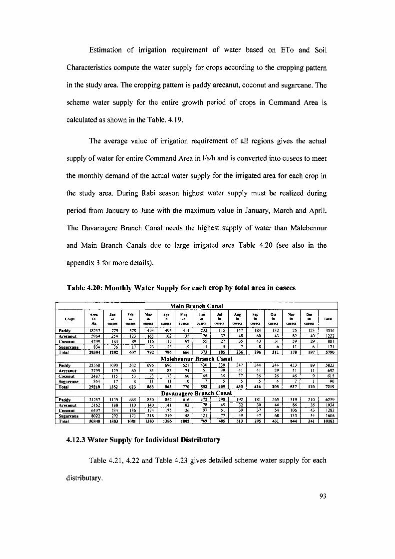
Estimation of irrigation requirement of water based on ETo and Soil

Characteristics compute the water supply for crops according to the cropping pattern

in the study area. The cropping pattern is paddy arecanut, coconut and sugarcane. The

scheme water supply for the entire growth period of crops in Command Area is

calculated as shown in the Table. 4.19.

The average value of irrigation requirement of all regions gives the actual

supply of water for entire Command Area in 1/s/h and is converted into cusecs to meet

the monthly demand of the actual water supply for the irrigated area for each crop in

the study area. During Rabi season highest water supply must be realized during

period from January to June with the maximum value in January, March and April.

The Davanagere Branch Canal needs the highest supply of water than Malebennur

and Main Branch Canals due to large irrigated area Table 4.20 (see also in the

appendix 3 for more details).

Table 4.20: Monthly Water Supply for each crop by total area in cusecs

Main Branch Canal

Crops Area

In Ha

Jan in

cusecs

Feb in

cusecs

Mar in

cusecs

Apr in

cusecs

May in

cusecs

Jun in

cusecs

Jul in

cusecs

Aug in

cusecs

Sep in

cusecs

Oct in

cusecs

Nov in

cusecs

Dec in

cusecs Total

Paddy 18257 779 378 493 495 414 232 115 147 184 132 25 123 3516

Arecanut 5964 254 123 161 162 135 76 37 48 60 43 82 40 1222

Coconut 4299 183 89 116 117 97 55 27 35 43 31 59 29 881

Sugarcane 834 36 17 23 23 19 11 5 7 8 6 11 6 171

Total 29354 1252 607 792 796 666 373 185 236 296 211 178 197 5790

Malebennur Branch Canal Paddy 23568 1090 502 696 696 621 430 330 347 344 244 433 89 5823

Arecanut 2799 129 60 83 83 74 51 39 41 41 29 51 11 692

Coconut 2487 115 53 73 73 66 45 35 37 36 26 46 9 615

Sugarcane 364 17 8 11 n 10 7 5 5 5 4 7 1 90

Total 29218 1352 623 863 863 770 533 409 430 426 303 537 110 7219

Davanagere Branch Canal Paddy 31257 1139 665 850 852 616 472 298 192 181 265 519 210 6259

Arecanut 5162 188 110 140 141 102 78 49 32 30 44 86 35 1034

Coconut 6407 234 136 174 175 126 97 61 39 37 54 106 43 1283

Sugarcane 8022 292 171 218 219 158 121 77 49 47 68 133 54 1606

Total 50848 1853 1081 1383 1386 1002 769 485 313 295 431 844 341 10182

4.12.3 Water Supply for Individual Distributary

Table 4.21, 4.22 and Table 4.23 gives detailed scheme water supply for each

distributary.

93

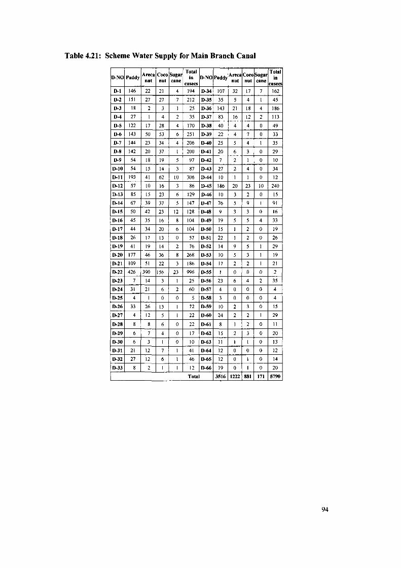
Table 4.21: Scheme Water Supply for Main Branch Canal

D-NO Paddy Areca nut

Coco nut

Sugar cane

Total in

cusecs D-NO Paddy

Areca nut

Coco nut

Sugar cane

Total in

cusecs

D-1 146 22 21 4 194 D-34 107 32 17 7 162

D-2 151 27 27 7 212 D-3S 35 5 4 1 45

D-3 18 2 3 1 25 D-36 143 21 18 4 186

D-4 27 1 4 2 35 D-37 83 16 12 2 113

D-5 122 17 28 4 170 D-38 40 4 4 0 49

D-6 143 50 53 6 251 D-39 22 4 7 0 33

D-7 144 23 34 4 206 D-40 25 5 4 1 35

D-8 142 20 37 1 200 EMI 20 6 3 0 29

D-9 54 18 19 5 97 D-42 7 2 1 0 10

D-10 54 15 14 3 87 D-43 27 2 4 0 34

D-11 193 41 62 10 306 D-44 10 1 1 0 12

D-12 57 10 16 3 86 0-45 186 20 23 10 240

D-13 85 15 23 6 129 D-46 10 3 2 0 15

D-14 67 39 37 5 147 D-47 76 5 9 1 91

D-IS 50 42 23 12 128 D-48 9 3 3 0 16

D-16 45 35 16 8 104 D-49 19 5 5 4 33

D-17 44 34 20 6 104 D-50 15 1 2 0 19

D-18 26 17 13 0 57 D-Sl 22 1 2 0 26

D-19 41 19 14 2 76 D-S2 14 9 5 1 29

D-20 177 46 36 8 268 D-53 10 5 3 1 19

D-21 109 51 22 3 186 D-54 17 2 2 1 21

D-22 426 390 156 23 996 D-55 1 0 0 0 2

D-23 7 14 3 1 25 D-56 23 6 4 2 35

D-24 31 21 6 2 60 D-57 4 0 0 0 4

D-25 4 1 0 0 5 D-58 3 0 0 0 4

D-26 33 26 13 1 72 D-S9 10 2 3 0 15

D-27 4 12 5 1 22 D-60 24 2 2 1 29

D-28 8 8 6 0 22 D-61 g 1 2 0 11

D-29 6 7 4 0 17 D-62 15 2 3 0 20

D-30 6 3 1 0 10 D-63 11 1 1 0 13

D-31 21 12 7 1 41 D-64 12 0 0 0 12

D-32 27 12 6 1 46 D-6S 12 0 1 0 14

D-33 8 2 1 1 12 D-66 19 0 1 0 20

Total 3516 1222 881 171 5790

94

Table 4.22: Scheme Water Supply for Malebennur Branch Canal

D NO

Distributaries details Paddy Areca nut

Coco nut

Sugar cane

Total in

cusecs 1 1" ZONE DISTY SA OFFTAKE - 0.5KM 7 5 1 1 13 2 2" ZONE DISTY SA OFFTAKE - 2.80KM 4 4 1 1 9 3 2" ZONE DISTY SA OFFTAKE - 27 13 7 4 51 4 2" ZONE DISTY SA OFFTAKE - 44 7 7 1 58 5 3'" ZONE DISTY SA OFFTAKE 53 11 7 1 72 6 3"* ZONE DISTY SA OFFTAKE - 5.20KM 42 5 6 0 54 7 4" ZONE DISTY SA OFFTAKE - 5.90KM 131 26 15 2 174 8 5* ZONE DISTY SA OFFTAKE - 8.80KM 128 31 25 3 187 9 6* ZONE DISTY SA OFFTAKE - 9.40KM 223 43 31 2 299 10 DRAFT CHANNEL BELOW ESCAPE OFFTAKE - 10 6 1 1 0 9 11 HAROSAGARA DISTRIBUTARY OF SA OFFTAKE 22 21 7 1 50 12 KOTEHALU TANK SLUICE OFFTAKE - I4.0KM 8 4 1 1 13 13 7* ZONE DISTY SA OFFTAKE - 14.70KM 53 26 11 2 91 14 P' ZONE DISTY MBC OFFTAKE -I6.60KM 264 23 26 2 314 15 2" ZONE DISTY MBC OFFTAKE - I7.90KM 14 12 4 2 32 16 3'" ZONE DISTY MBC OFFTAKE - 19.40KM 258 47 35 2 342 17 4* ZONE DISTY MBC OFFTAKE - 21.70KM 623 59 66 6 754 18 5* ZONE DISTY MBC OFFTAKE - 22.30KM 124 10 12 0 146 19 DIS-16B-N0 DETAIL 6 1 1 0 8 20 KUNDUR TANK SLUICE OFFTAKE - 24.40KM 14 3 2 1 20 21 6* ZONE DISTY MBC OFFTAKE - 26.30KM 247 24 20 2 292 22 6* ZONE DISTY MBC OFFTAKE 15 3 2 0 20 23 7* ZONE DISTY MBC OFFTAKE - 29.80KM 62 5 5 0 73 24 gih gih 20NE DISTY MBC OFFTAKE - 3 962 97 94 6 1159 25 DHLS OFFTAKE - 32.60KM 2 1 1 0 4 26 9* ZONE DISTY OFFTAKE - 3 14 4 3 0 21 27 10* ZONE DISTY OFFTAKE - 36.10KM 442 40 48 3 535 28 10* ZONE DISTY OFFTAKE - 11 1 2 0 15 29 11* ZONE DISTY OFFTAKE - 124 20 24 2 171

L-30 12* ZONE DISTY OFFTAKE- 233 28 34 5 301 L-31 12* ZONE DISTY OFFTAKE - 38.10KM 33 5 7 0 45 R-32 11* ZONE DISTY OFFTAKE- 54 4 4 1 62 L-33 13* ZONE DISTY OFFTAKE - 42.60KM 423 19 23 3 468 R-34 11* ZONE DISTY OFFTAKE - 38 6 4 2 50 L-35 14* ZONE DISTY OFFTAKE - 43.80KM 259 29 24 4 315 R-36 11* ZONE DISTY OFFTAKE - 73 7 6 1 87 R-37 11* ZONE DISTY OFFTAKE - 61 1 2 0 65 L-38 15* ZONE DISTY OFFTAKE - 45.90KM 326 15 22 6 370 R-39 11* ZONE DISTY OFFTAKE- 50 1 0 1 52 L-40 16* ZONE DISTY OFFTAKE - 47.80KM 164 16 17 10 207 L-41 17* ZONE DISTY OFFTAKE - 47.80KM 20 1 1 1 22 R-42 17* ZONE DISTY OFFTAKE - 47.80KM 158 12 5 12 187

Total 5823 692 615 90 7219

95

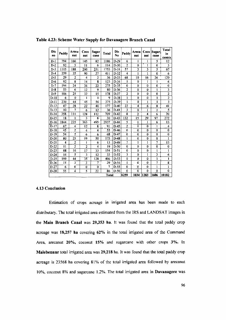
Table 4.23: Scheme Water Supply for Davanagere Branch Canal

Dis no

Paddy Areca nut

Coco nut

Sugar cane

Total Dis No

Paddy Areca nut

Coco nut

Sugar cane

Total in

cu$ecs D-1 794 166 145 82 1186 D-29 6 1 1 5 12 D-2 92 5 11 6 114 D-30 2 0 1 0 3 D-3 1115 188 200 251 1753 D-31 57 3 3 5 67 D-4 259 35 90 27 411 D-32 4 1 1 0 6 D-5 29 2 4 2 36 D-33 68 10 16 26 120 D-6 92 8 14 8 123 D-34 5 0 1 1 6 D-7 194 24 36 22 275 D-35 0 0 0 0 0 D-8 53 6 12 9 80 D-36 2 0 0 1 3 D-9 106 25 32 15 178 D-37 2 0 0 0 2 D-10 6 0 1 1 9 D-38 1 0 0 1 2 D-11 230 44 45 56 375 D-39 1 0 1 1 3 D-I2 87 28 22 40 177 D-40 22 4 6 8 41 D-13 10 7 6 12 36 D-41 3 0 1 1 5 D-14 358 111 128 112 709 D-42 8 2 4 6 20 D-15 18 1 3 8 30 D-43 132 15 29 97 272 D-16 1844 235 363 495 2937 D-44 5 1 1 6 13 D-17 67 4 12 8 91 D-45 2 1 0 1 4 D-18 45 2 4 4 55 D-46 0 0 0 0 0 D-19 54 2 6 6 68 D-47 0 0 0 0 0 D-20 80 25 19 50 175 D-48 1 0 0 0 1 D-21 4 2 1 6 13 D-49 7 1 1 7 15 D-22 11 2 2 4 19 D-50 0 0 0 0 0 D-23 88 16 17 33 154 D-51 0 0 0 1 1 D-24 14 5 3 12 33 D-52 3 0 1 3 6 D-25 199 44 35 128 406 D-53 0 0 0 1 1 D-26 15 3 3 7 29 D-54 I 0 0 7 8 D-27 6 0 0 0 7 D-55 0 0 0 1 1 D-28 55 4 5 22 86 D-56 0 0 0 0 0

Total 6259 1034 1283 1606 10182

4.13 Conclusion

Estimation of crops acreage in irrigated area has been made to each

distributary. The total irrigated area estimated from the IRS and LANDSAT images in

the Main Branch Canal was 29,353 ha. It was found that the total paddy crop

acreage was 18,257 ha covering 62% in the total irrigated area of the Command

Area, arecanut 20%, coconut 15% and sugarcane with other crops 3%. In

Malebennur total irrigated area was 29,218 ha. It was found that the total paddy crop

acreage is 23568 ha covering 81% of the total irrigated area followed by arecanut

10%, coconut 8% and sugarcane 1.2%. The total irrigated area in Davanagere was

96

50,848 ha and it is found that the total paddy crop acreage was 31,257 ha covering

62% of the total irrigated area followed by sugarcane 15%, coconut 13% and arecanut

10%.

CROPWAT modeling approach is very useful for evaluating crop water

requirement and analysis of scheme supply in the study area. The outputs of

CROPWAT model confirms that there is an increase in reference crop

evapotranspiration (ETo) in Rabi season, which is basically due to the impact of local

climate and crop evapotranspiration (ETc). The average crop-water demand during

Rabi season for paddy is 1,159 mm/season (Table 4.17) and for annual crops 1,267,62

mm/year, 1,564.22 mm/year and 1,582.03 mm/year for arecanut coconut, and sugarcane

respectively (Table 4.18).

To meet its demand of irrigation water requirement in the Main Branch

Canal should require about 5,790 cusecs which equal to 0.1972541 cusecs per ha.

Malebennur Branch Canal require a total water supply for crops in the entire

Command Area annually which must be 7,219 cusecs, which equals 0.24707 cusecs

per ha. Davanagere Branch Canal requires water supply of 10,181.5 which is about

0.20023 cusecs per ha.

4.13.1 ETc and ETo vs Rainfall

The evapotranspiration is the most important component of water balance.

This is estimated as the product of cropped area irrigated and crop evapotranspiration

(ETc) for each crop based on climatological data and the crop coefficient (Kc), which

is specific to each crop grown and cropping acreage. The quantity of water consumed

as evapotranspiration from the crops in the Command Area such as arecanut, coconut,

sugarcane, and paddy are the highest in March, April, and the peak value in May with

97

low rainfall (Fig 4.9). On the other hand from June to October the ETc and ETo are

high and also the rainfall with monthly average between 123 mm to 124 mm.

S S

s I

350

300

250

200

150

100

50

0

Jan Feb Mar Apr May Jun Jul Aug Sep Oct Nov Dec • ETc "Rainfall » ETo

Figure 4.9: ETc and ETo vs Rainfall

In both cases, the area located under deficit situation against crop water

requirement with less rainfall, it is of critical importance to issue more water during

January to May.

98