chapter 2 supply and demand talk is cheap because supply exceeds demand

Chapter 2

Supply and Demand

Talk is cheap because supply exceeds demand.

Copyright ©2014 Pearson Education, Inc. All rights reserved. 2-2

Chapter 2 Outline

Challenge: Quantities and Prices of Genetically Modified Foods

2.1 Demand2.2 Supply2.3 Market Equilibrium2.4 Shocking the Equilibrium: Comparative

Statistics2.5 Elasticities2.6 Effects of a Sales Tax2.7 Quantity Supplied Need Not Equal Quantity

Demanded2.8 When to Use the Supply-and-Demand Model

Challenge Solution


Challenge: Quantities and Prices of Genetically Modified Foods

• Background:• The decision whether to permit firms to grow and

sell genetically modified (GM) foods affects the supply and demand for food.

• Questions: • Will the use of GM seeds lead to lower prices and

more food sold?• What happens to prices and quantities sold if

consumers refuse to buy GM crops?


2.1 Demand

• The quantity of a good or service that consumers demand depends on price and other factors such as consumers’ incomes and the prices of related goods.

• The demand function describes the mathematical relationship between quantity demanded (Qd), price (p) and other factors that influence purchases:

• p = per unit price of the good or service

• ps = per unit price of a substitute good

• pc = per unit price of a complementary good

• Y = consumers’ income


2.1 Demand

• We often work with a linear demand function.• Example: estimated demand function for pork in Canada.

• Qd = quantity of pork demanded (million kg per year)

• p = price of pork (in Canadian dollars per kg)

• pb = price of beef, a substitute good (in Canadian dollars per kg)

• pc = price of chicken, another substitute (in Canadian dollars per kg)

• Y = consumers’ income (in Canadian dollars per year)

• Graphically, we can only depict the relationship between Qd and p, so we hold the other factors constant.


2.1 Demand Example: Canadian Pork

Assumptions about pb, pc, and Y to simplify equation

• pb = $4/kg

• pc = $3.33/kg

• Y = $12.5 thousand


2.1 Demand Example: Canadian Pork

• Changing the own-price of pork simply moves us along an existing demand curve.

• Changing one of the things held constant (e.g. pb, pc, and Y) shifts the entire demand curve.

• pb to $4.60 /kg


2.2 Supply

• The quantity of a good or service that firms supply depends on price and other factors such as the cost of inputs that firms use to produce the good or service.

• The supply function describes the mathematical relationship between quantity supplied (Qs), price (p) and other factors that influence the number of units offered for sale:

• p = per unit price of the good or service

• ph = per unit price of other production factors


2.2 Supply

• We often work with a linear supply function.• Example: estimated supply function for pork in Canada.

• Qs = quantity of pork supplied (million kg per year)

• p = price of pork (in Canadian dollars per kg)

• ph = price of hogs, an input (in Canadian dollars per kg)

• Graphically, we can only depict the relationship between Qs and p, so we hold the other factors constant.


2.2 Supply Example: Canadian Pork

• Assumption about ph to simplify equation

• ph = $1.50/kg

40dp

dQs slopedQ

dp

s

40

1


2.2 Supply Example: Canadian Pork

• Changing the own-price of pork simply moves us along an existing supply curve.

• Changing one of the things held constant (e.g. ph) shifts the entire supply curve.

• ph to $4.60 /kg


2.2 Summing Supply Functions Example: Domestic and Foreign Supply of Rice


2.3 Market Equilibrium

• The interaction between consumers’ demand curve and firms’ supply curve determines the market price and quantity of a good or service that is bought and sold.

• Mathematically, we find the price that equates the quantity demanded, Qd, and the quantity supplied, Qs:• Given and , find p such that

Qd = Qs:

p = $3.30

pQd 20286 pQs 4088pp 408820286


2.3 Market Equilibrium

• Graphically, market equilibrium occurs where the demand and supply curves intersect.• At any other price, excess supply or excess

demand results.• Natural market forces push toward equilibrium Q

and p.

Stephanie Lindsey

missing the lines in the artwork on the bottom left.


2.4 Shocking the Equilibrium: Comparative Statics

• Changes in a factor that affects demand, supply, or a new government policy alters the market price and quantity of a good or service.

• Changes in demand and supply factors can be analyzed graphically and/or mathematically.• Graphical analysis should be familiar from your

introductory microeconomics course.• Mathematical analysis simply utilizes demand and

supply functions to solve for a new market equilibrium.• Changes in demand and supply factors can be large or

small.• Small changes are analyzed with calculus.


2.4 Shocking the Equilibrium: Comparative Statics with Discrete (Relatively Large) Changes

• Graphically analyzing the effect of an increase in the price of hogs• When an input gets more expensive, producers

supply less pork at every price.


2.4 Shocking the Equilibrium: Comparative Statics with Discrete (Relatively Large) Changes

• Mathematically analyzing the effect of an increase in the price of hogs• If ph increases by $0.25, new ph = $1.75 and

pQs 4073

55.3$

407320286

p

pp

QQ sd 21555.320286 dQ

21555.34073 sQ


2.4 Shocking the Equilibrium: Comparative Statics with Small Changes

• Demand and supply functions are written as general functions of the price of the good, holding all else constant:

• Supply is also a function of some exogenous (not in firms’ control) variable, a:

• Because the intersection of demand and supply determines the price, p, we can write the price as an implicit function of the supply-shifter, a:

• In equilibrium: ( ),Q S p a a


2.4 Shocking the Equilibrium: Comparative Statics with Small Changes

• Given the equilibrium condition , we differentiate with respect to a using the chain rule to determine how equilibrium is affected by a small change in a:

• Rearranging:


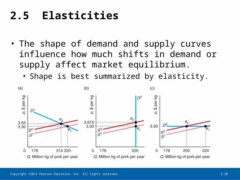
2.5 Elasticities

• The shape of demand and supply curves influence how much shifts in demand or supply affect market equilibrium.• Shape is best summarized by elasticity.


2.5 Elasticities

• Elasticity indicates how responsive one variable is to a change in another variable.

• The price elasticity of demand measures how sensitive the quantity demanded of a good, Qd, is to changes in the price of that good, p.

• If , then and elasticity can be evaluated at any point on the demand curve.

bpaQd


2.5 Example: Elasticity of Demand

• Previous pork demand was• Calculating price elasticity of demand at

equilibrium (p=$3.30 and Q=220):

• Interpretation:• negative sign consistent with downward-sloping

demand• a 1% increase in the price of pork leads to a 0.3%

decrease in quantity of pork demanded

pQd 20286


2.5 Demand Elasticity

• Elasticity of demand varies along a linear demand curve


2.5 Demand Elasticity

• On a given supply curve, elasticity of demand remains constant


2.5 Elasticities

• There are other common elasticities that are used to gauge responsiveness.• income elasticity of demand

• cross-price elasticity of demand

• elasticity of supply


2.5 Constant Elasticity of Supply Curve

• On a given supply curve, elasticity of supply is constant.


2.6 Effects of a Sales Tax

• Two types of sales taxes:• Ad valorem tax is in percentage terms

• California’s state tax rate is 8.25%, so a $100 purchase generates $8.25 in tax revenue

• Specific (or unit) tax is in dollar terms• U.S. gasoline tax is $0.18 per gallon

• Ad valorem taxes are much more common.

• The effect of a sales tax on equilibrium price and quantity depends on elasticities of demand and supply.


2.6 Equilibrium Effects of a Specific Tax

• Consider the effect of a $1.05 per unit (specific) sales tax on the pork market that is collected from pork producers.


2.6 How Specific Tax Effects Depend on Elasticities

• If a unit tax, , is collected from pork producers, the price received by pork producers is reduced by this amount and our equilibrium condition becomes:

• Differentiating with respect to :

• Rearranging indicates how the tax changes the price consumers pay:


2.6 How Specific Tax Effects Depend on Elasticities

• The equation can be expressed in terms of elasticities by multiplying through by p/Q:

• Tax incidence on consumers, the amount by which the price to consumers rises as a fraction of the amount of the tax, is now easy to calculate given elasticities of demand and supply.

• Tax incidence on firms, the amount by which the price paid to firms rises, is simply 1 – dp/d


2.6 Important Questions About Tax Effects

• Does it matter whether the tax is collected from producers or consumers?• Tax incidence is not sensitive to who is actually taxed.• A tax collected from producers shifts the supply curve back.• A tax collected from consumers shifts the demand curve

back.• Under either scenario, a tax-sized wedge opens up between

demand and supply and the incidence analysis is identical.

• Does it matter whether the tax is a unit tax or an ad valorem tax?• If the ad valorem tax rate is chosen to match the per unit tax

divided by equilibrium price, the effects are the same.


2.6 Important Questions About Tax Effects

• Does it matter whether the tax is a unit tax or an ad valorem tax?


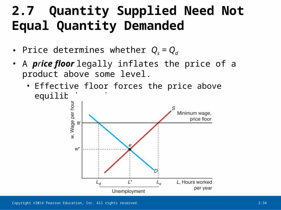
2.7 Quantity Supplied Need Not Equal Quantity Demanded

• Price determines whether Qs = Qd

• A price ceiling legally limits the amount that can be charged for a product.• Effective ceilings force the price below equilibrium price.


2.7 Quantity Supplied Need Not Equal Quantity Demanded

• Price determines whether Qs = Qd

• A price floor legally inflates the price of a product above some level.• Effective floor forces the price above equilibrium price.


2.8 When to Use the Supply-and-Demand Model

• This model is appropriate in markets that are perfectly competitive:1. There are a large number of buyers and sellers.2. All firms produce identical products.3. All market participants have full information

about prices and product characteristics.4. Transaction costs are negligible.5. Firms can easily enter and exit the market.

• We will talk more about the perfectly competitive market in Chapter 8.


Challenge Solution

• With the introduction of GM foods, supply increases and demand decreases. For a given increase in supply, the effect of the decrease in demand on the equilibrium price and quantity depends on the magnitude of the shift in demand.

chapter 2 supply and demand talk is cheap because supply exceeds demand

Documents

price p

price of pork

year p

consumers demand

demand example

unit price

service p s

substitute good p c