chapter 2 bifurcations -...

Chapter 2

Bifurcations

In the previous chapter we discuss the fact that disspatives systems possess attractors.Generally, in a model, the vector field ~F depends on parameters and the behavior of thesystem may depend on the values of those parameters. It means that the the numberand/or nature of attractors may change when parameters are tuned. Such a change iscalled a bifurcation. The value of the parameter for which such qualitative change ofthe structure of the phase space happens is called the critical value of the parameter.

The bifurcation theory studies this problem for any numbers of parameters. Here wewill study only the simple case of a vector field ~F depending only on one parameter.Moreover, we will only study the cases where a limited part of the phase space is involvedin the change. Those particular kind of bifurcations are local and of codimension 1.

Near a bifurcation, the dynamical system can be reduced to a generic mathematicalform by a change of variables and a reduction of its dimension to keep only the directionsimplied in the bifurcation. Those reduced mathematical expressions are called normalforms and each form is associated to a type of bifurcation.

2.1 Saddle-node bifurcation

This bifurcation corresponds to the apparition or anihilation of a pair of fixed points. Itsnormal form is:

x = µ− x2

where x ∈ R.

The study of the stability of the normal form gives two fixed points ±√µ whichcan exist only when µ ≥ 0. As ∂F

∂x= −2x, we obtain ∂F

∂x|+√µ = −2

√µ < 0 and

∂F∂x|−√µ = 2

√µ > 0 so that the fixed point +

√µ is stable and the other one −√µ is

unstable.

47

48 CHAPTER 2. BIFURCATIONS

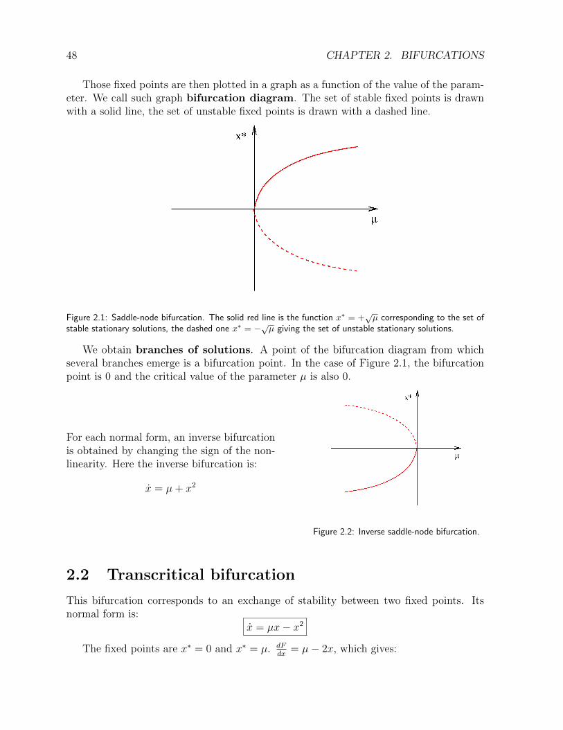
Those fixed points are then plotted in a graph as a function of the value of the param-eter. We call such graph bifurcation diagram. The set of stable fixed points is drawnwith a solid line, the set of unstable fixed points is drawn with a dashed line.

Figure 2.1: Saddle-node bifurcation. The solid red line is the function x∗ = +√µ corresponding to the set of

stable stationary solutions, the dashed one x∗ = −√µ giving the set of unstable stationary solutions.

We obtain branches of solutions. A point of the bifurcation diagram from whichseveral branches emerge is a bifurcation point. In the case of Figure 2.1, the bifurcationpoint is 0 and the critical value of the parameter µ is also 0.

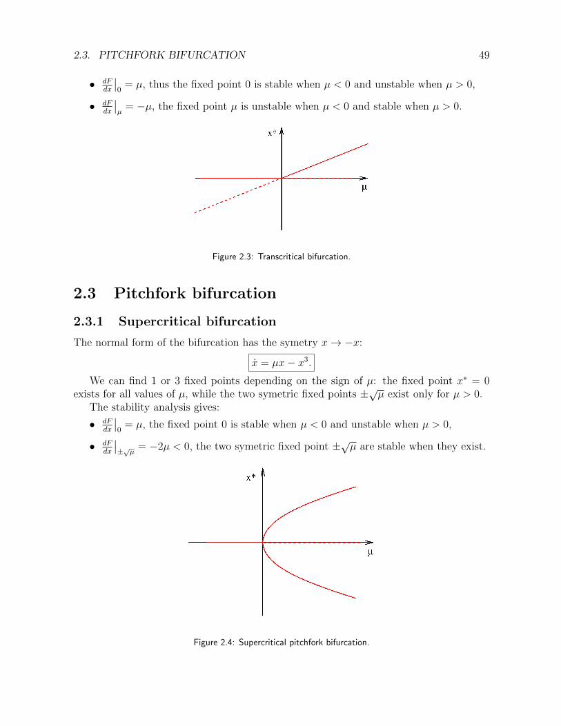
For each normal form, an inverse bifurcationis obtained by changing the sign of the non-linearity. Here the inverse bifurcation is:

x = µ+ x2

Figure 2.2: Inverse saddle-node bifurcation.

2.2 Transcritical bifurcation

This bifurcation corresponds to an exchange of stability between two fixed points. Itsnormal form is:

x = µx− x2

The fixed points are x∗ = 0 and x∗ = µ. dFdx

= µ− 2x, which gives:

2.3. PITCHFORK BIFURCATION 49

• dFdx

∣∣0

= µ, thus the fixed point 0 is stable when µ < 0 and unstable when µ > 0,

• dFdx

∣∣µ

= −µ, the fixed point µ is unstable when µ < 0 and stable when µ > 0.

Figure 2.3: Transcritical bifurcation.

2.3 Pitchfork bifurcation

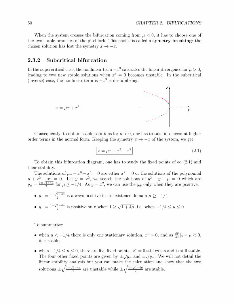
2.3.1 Supercritical bifurcation

The normal form of the bifurcation has the symetry x→ −x:

x = µx− x3.

We can find 1 or 3 fixed points depending on the sign of µ: the fixed point x∗ = 0exists for all values of µ, while the two symetric fixed points ±√µ exist only for µ > 0.

The stability analysis gives:

• dFdx

∣∣0

= µ, the fixed point 0 is stable when µ < 0 and unstable when µ > 0,

• dFdx

∣∣±√µ = −2µ < 0, the two symetric fixed point ±√µ are stable when they exist.

Figure 2.4: Supercritical pitchfork bifurcation.


When the system crosses the bifurcation coming from µ < 0, it has to choose one ofthe two stable branches of the pitchfork. This choice is called a symetry breaking: thechosen solution has lost the symetry x→ −x.

2.3.2 Subcritical bifurcation

In the supercritical case, the nonlinear term −x3 saturates the linear divergence for µ > 0,leading to two new stable solutions when x∗ = 0 becomes unstable. In the subcritical(inverse) case, the nonlinear term is +x3 is destabilizing:

x = µx+ x3

Consequently, to obtain stable solutions for µ > 0, one has to take into account higherorder terms in the normal form. Keeping the symetry x→ −x of the system, we get:

x = µx+ x3 − x5 (2.1)

To obtain this bifurcation diagram, one has to study the fixed points of eq (2.1) andtheir stability.

The solutions of µx+ x3− x5 = 0 are either x∗ = 0 or the solutions of the polynomialµ + x2 − x4 = 0. Let y = x2, we search the solutions of y2 − y − µ = 0 which arey± = 1±

√1+4µ2

for µ ≥ −1/4. As y = x2, we can use the y± only when they are positive.

• y+ = 1+√

1+4µ2

is always positive in its existence domain µ ≥ −1/4

• y− = 1−√

1+4µ2

is positive only when 1 ≥√

1 + 4µ, i.e. when −1/4 ≤ µ ≤ 0.

To summarize:

• when µ < −1/4 there is only one stationary solution, x∗ = 0, and as dFdx|0 = µ < 0,

it is stable.

• when −1/4 ≤ µ ≤ 0, there are five fixed points. x∗ = 0 still exists and is still stable.The four other fixed points are given by ±√y+ and ±√y−. We will not detail thelinear stability analysis but you can make the calculation and show that the two

solutions ±√

1−√

1+4µ2

are unstable while ±√

1+√

1+4µ2

are stable.

2.4. HOPF BIFURCATION 51

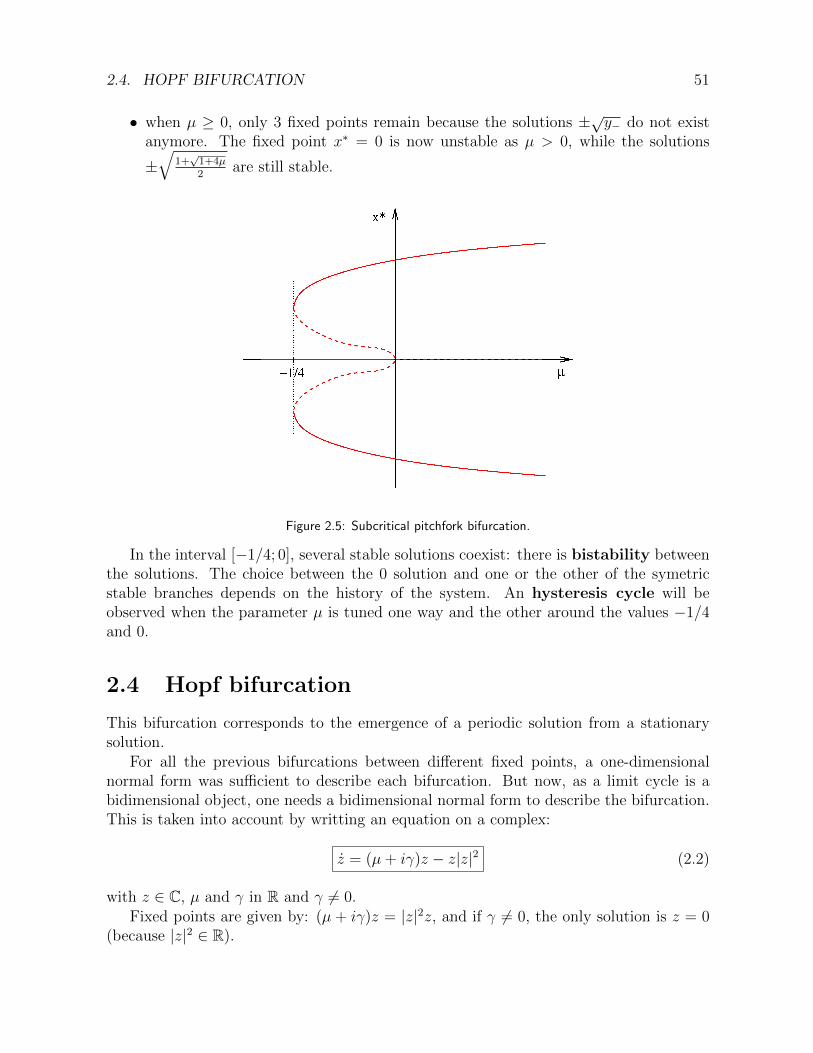
• when µ ≥ 0, only 3 fixed points remain because the solutions ±√y− do not existanymore. The fixed point x∗ = 0 is now unstable as µ > 0, while the solutions

±√

1+√

1+4µ2

are still stable.

Figure 2.5: Subcritical pitchfork bifurcation.

In the interval [−1/4; 0], several stable solutions coexist: there is bistability betweenthe solutions. The choice between the 0 solution and one or the other of the symetricstable branches depends on the history of the system. An hysteresis cycle will beobserved when the parameter µ is tuned one way and the other around the values −1/4and 0.

2.4 Hopf bifurcation

This bifurcation corresponds to the emergence of a periodic solution from a stationarysolution.

For all the previous bifurcations between different fixed points, a one-dimensionalnormal form was sufficient to describe each bifurcation. But now, as a limit cycle is abidimensional object, one needs a bidimensional normal form to describe the bifurcation.This is taken into account by writting an equation on a complex:

z = (µ+ iγ)z − z|z|2 (2.2)

with z ∈ C, µ and γ in R and γ 6= 0.Fixed points are given by: (µ + iγ)z = |z|2z, and if γ 6= 0, the only solution is z = 0

(because |z|2 ∈ R).


To do the linear stability analysis, we want more conventional writting of the equationswith two equations on variables in R. Writing z = x+ iy, we have:{

x = µx− γy − x(x2 + y2)y = µy + γx− y(x2 + y2)

The linearization in (0, 0) gives

L|(0,0) =

[µ −γγ µ

],

from which we deduce ∆ = µ2 + γ2 > 0 and T = 2µ. Consequently, the fixed point (0, 0)is stable for µ < 0 and unstable for µ > 0. At the bifurcation, the behavior around thefixed point changes from a convergent spiral to a divergent spiral. To understand whathappens to the trajectories when µ > 0, we use the other decomposition of a complexnumber with modulus and phase: z = reiθ which gives:{

r = µr − r3

θ = γ

We recognize for the evolution of the modulus the normal form of a supercritical pitchforkbifurcation, while the phase has a linear dependence in time. We deduce from this systemthat the stable solution for µ > 0 is a solution of fixed modulus but linearly increasingphase with time. It is a periodic solution which verifies r =

√µ and θ = γt + θ0. The

bifurcation diagram of a Hopf bifurcation is given in Figure 2.6.

Figure 2.6: Hopf bifurcation.

The subcritical case exists: z = (µ + iγ)z + z|z|2. The study is exactly the same asthe supercritical case, leading to unstable limit cycles solution for µ < 0.

2.5. IMPERFECT BIFURCATION. INTRODUCTION TO CATASTROPHE THEORY53

2.5 Imperfect bifurcation. Introduction to catastro-

phe theory

Bibliography:

• Nonlinear dynamics and chaos, S. Strogatz,

• Dynamiques complexes et morphogenese, C. Misbah.

Coming back to the pitchfork bifurcation, you can have the intuition that the bifur-cation diagram we draw was idealized and that in fact, in a real system a branch will bealways chosen preferentially because of some imperfection of the system.

This problematic deals with the question of the robustness of the model to a pertur-bation (note that we speak of the perturbation of the model and not of a given solutionof the equations).

In this part, we want to know how the pitchfork bifurcation will be modified if a newparameter h is added to its normal form:

x = µx− x3 + h

Do we observe the same qualitative bifurcation or not ? Does it keep its general proper-ties ?

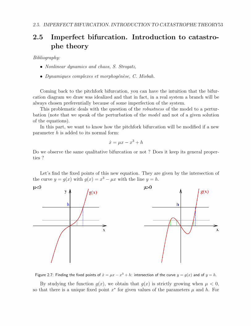
Let’s find the fixed points of this new equation. They are given by the intersection ofthe curve y = g(x) with g(x) = x3 − µx with the line y = h.

Figure 2.7: Finding the fixed points of x = µx− x3 + h: intersection of the curve y = g(x) and of y = h.

By studying the function g(x), we obtain that g(x) is strictly growing when µ < 0,so that there is a unique fixed point x∗ for given values of the parameters µ and h. For


µ > 0, the derivative of g(x) is negative in the interval [−√

µ3,+√

µ3], so that depending

on the value of h, we can find either 1 or 3 fixed points (respectively blue and green caseson the right part of Figure 2.7). A straightforward calculation gives that we find 3 fixedpoints when h ∈ [−2µ

3

√µ3,+2µ

3

√µ3], while for values of h outside this interval there is

only one fixed point.

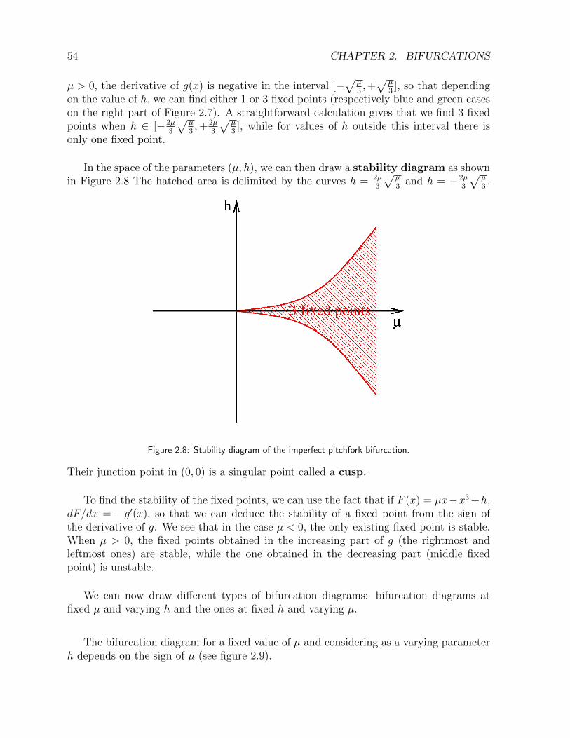
In the space of the parameters (µ, h), we can then draw a stability diagram as shownin Figure 2.8 The hatched area is delimited by the curves h = 2µ

3

√µ3

and h = −2µ3

√µ3.

Figure 2.8: Stability diagram of the imperfect pitchfork bifurcation.

Their junction point in (0, 0) is a singular point called a cusp.

To find the stability of the fixed points, we can use the fact that if F (x) = µx−x3 +h,dF/dx = −g′(x), so that we can deduce the stability of a fixed point from the sign ofthe derivative of g. We see that in the case µ < 0, the only existing fixed point is stable.When µ > 0, the fixed points obtained in the increasing part of g (the rightmost andleftmost ones) are stable, while the one obtained in the decreasing part (middle fixedpoint) is unstable.

We can now draw different types of bifurcation diagrams: bifurcation diagrams atfixed µ and varying h and the ones at fixed h and varying µ.

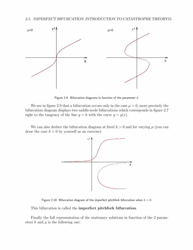
The bifurcation diagram for a fixed value of µ and considering as a varying parameterh depends on the sign of µ (see figure 2.9).

2.5. IMPERFECT BIFURCATION. INTRODUCTION TO CATASTROPHE THEORY55

Figure 2.9: Bifurcation diagrams in function of the parameter h.

We see in figure 2.9 that a bifurcation occurs only in the case µ > 0, more precisely thebifurcation diagram displays two saddle-node bifurcations which corresponds in figure 2.7right to the tangency of the line y = h with the curve y = g(x).

We can also deduce the bifurcation diagram at fixed h > 0 and for varying µ (you candraw the case h < 0 by yourself as an exercise):

Figure 2.10: Bifurcation diagram of the imperfect pitchfork bifurcation when h > 0.

This bifurcation is called the imperfect pitchfork bifurcation.

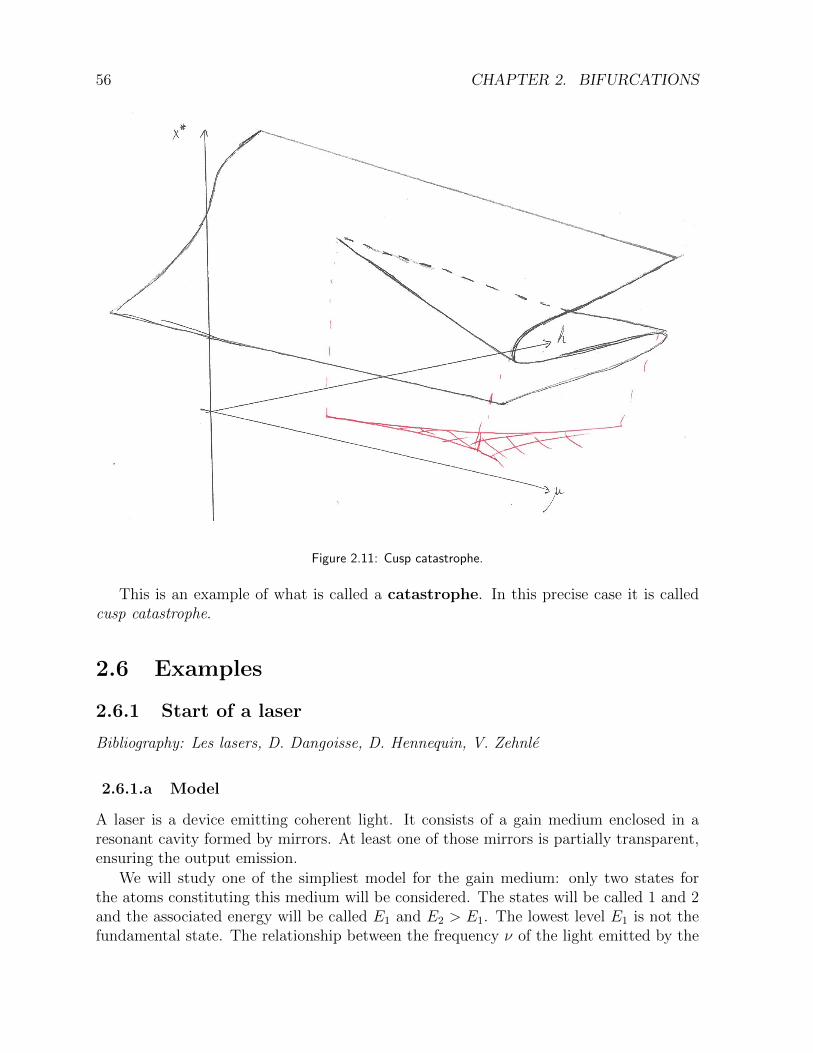
Finally the full representation of the stationary solutions in function of the 2 param-eters h and µ is the following one:


Figure 2.11: Cusp catastrophe.

This is an example of what is called a catastrophe. In this precise case it is calledcusp catastrophe.

2.6 Examples

2.6.1 Start of a laser

Bibliography: Les lasers, D. Dangoisse, D. Hennequin, V. Zehnle

2.6.1.a Model

A laser is a device emitting coherent light. It consists of a gain medium enclosed in aresonant cavity formed by mirrors. At least one of those mirrors is partially transparent,ensuring the output emission.

We will study one of the simpliest model for the gain medium: only two states forthe atoms constituting this medium will be considered. The states will be called 1 and 2and the associated energy will be called E1 and E2 > E1. The lowest level E1 is not thefundamental state. The relationship between the frequency ν of the light emitted by the

2.6. EXAMPLES 57

laser and the energy gap E2 − E1 is :

E2 − E1 = ~ω = hν.

Let’s defined the following variables :

• N1(t) is the number of atoms in the state 1 per unit volum at time t,

• N2(t) is the number of atoms in the state 2 per unit volum at time t,

• I(t) is the photons flux in the gain medium, i.e. the number of photons crossing aunit surface by unit time.

The mechanisms governing the light emission and absorption have been described byA. Einstein in 1916 :

• absorption :

During this process, a photon of energy hν is absorbed and an atom switches fromstate 1 to state 2. The number of atoms shifting from state 1 to state 2 is thusproportional to N1 and I. The proportionality coefficient has the dimension of asurface, it is called the absorption cross section and will be noted σa. Consequently,we have for the variation of the population of atoms in each states between times tand t+ ∆t :

(∆N2)abs = σaIN1∆t

(∆N1)abs = −σaIN1∆t

To calculate the variation of the photons flux, we consider a cylinder in the gainmedium along the direction propagation of the photons :


Per unit time, I(t)S photons enter in the volume Sc∆t and I(t + ∆t)S photonsexit. Besides, σaIN1 photons are absorbed per unit time and unit volume, so:

I(t+ ∆t)S − I(t)S = −(σaIN1)(c∆tS)

(∆I)abs = −σaIN1c∆t

• Stimulated emission: symetrically to the process of absorption, there is emissionof photons stimulated by photons already present in the cavity:

It is very important to note that this emission is not spontaneous : the photonsthat are generated when the atoms decay from state 2 to state 1 are clones of thephotons already present in the gain medium. They share all the properties of thephoton that have stimulated the emission, in particular its wave vector. We havefor the variations of the quantities that describe our system:

(∆N2)sti = −σstiIN2∆t

(∆N1)sti = σstiIN2∆t

(∆I)sti = σstiIN2c∆t

In the case considered here, we have σsti = σa = σ.

• Losses and decay: Independantly of the presence of photons already in the cavity,atoms which are not in the fundamental state tend to decay spontaneously towardslower states by emitting photons which are not coherent with the ones constitutingthe photons flux and consequently do not contribute to I. Atoms may also decayby other modes than the emission of photons: collisions, vibrations... For the sake

2.6. EXAMPLES 59

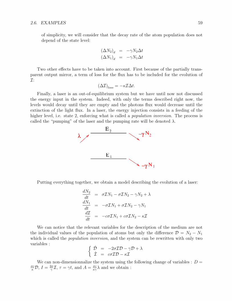
of simplicity, we will consider that the decay rate of the atom population does notdepend of the state level:

(∆N2)d = −γN2∆t

(∆N1)d = −γN1∆t

Two other effects have to be taken into account. First because of the partially trans-parent output mirror, a term of loss for the flux has to be included for the evolution ofI:

(∆I)loss = −κI∆t.

Finally, a laser is an out-of-equilibrium system but we have until now not discussedthe energy input in the system. Indeed, with only the terms described right now, thelevels would decay until they are empty and the photons flux would decrease until theextinction of the light flux. In a laser, the energy injection consists in a feeding of thehigher level, i.e. state 2, enforcing what is called a population inversion. The process iscalled the “pumping” of the laser and the pumping rate will be denoted λ.

Putting everything together, we obtain a model describing the evolution of a laser:

dN2

dt= σIN1 − σIN2 − γN2 + λ

dN1

dt= −σIN1 + σIN2 − γN1

dIdt

= −cσIN1 + cσIN2 − κI

We can notice that the relevant variables for the description of the medium are notthe individual values of the population of atoms but only the difference D = N2 − N1

which is called the population inversion, and the system can be rewritten with only twovariables : {

D = −2σID − γD + λ

I = cσID − κIWe can non-dimensionnalize the system using the following change of variables : D =

σcκD, I = 2σ

γI, τ = γt, and A = σc

κγλ and we obtain :


{D = −D(I + 1) + A

I = kI(D − 1)

where the time variable governing the derivatives is now τ and the control parameter is A,the pumping parameter. Indeed it corresponds to the parameter that can generally easilybe tuned experimentally, for example by the variation of an electrical current which isused to excite the atoms to a higher state, or any other mean of pumping. The parameterk depends of the loss of the mirrors through κ and of the gain medium through γ, so thatthis parameter is constant for a given laser.

2.6.1.b Study of the dynamical system

We thus have to study the dynamical system of dimension 2:{D = −D(I + 1) + A

I = kI(D − 1)

Fixed points {A = D(I + 1)0 = I(D − 1)

There are two fixed points:

• I = 0 and D = A, the laser is not emitting any light.

• D = 1 and I = A − 1, the light flux increases with the pumping while thepopulation inversion is saturated to a constant value.

Jacobian matrix

L =

(−(I + 1) −D

kI k(D − 1)

)Stability of (D = A, I = 0)

L|(A,0) =

(−1 −A0 k(A− 1)

)The trace is T = k(A− 1)− 1 and the determinant ∆ = −k(A− 1).

• when A < 1, ∆ > 0 and T < 0, the fixed point is stable.

• when A > 1, ∆ < 0, the fixed point is a saddle point and is unstable.

2.6. EXAMPLES 61

Stability of (D = 1, I = A− 1)

L|(1,A−1) =

(−A −1

k(A− 1) 0

)The trace T = −A is always negative and the determinant is ∆ = k(A− 1).

• when A < 1, ∆ < 0 the fixed point is a saddle point and is unstable.

• when A > 1, ∆ > 0, the fixed point is stable.

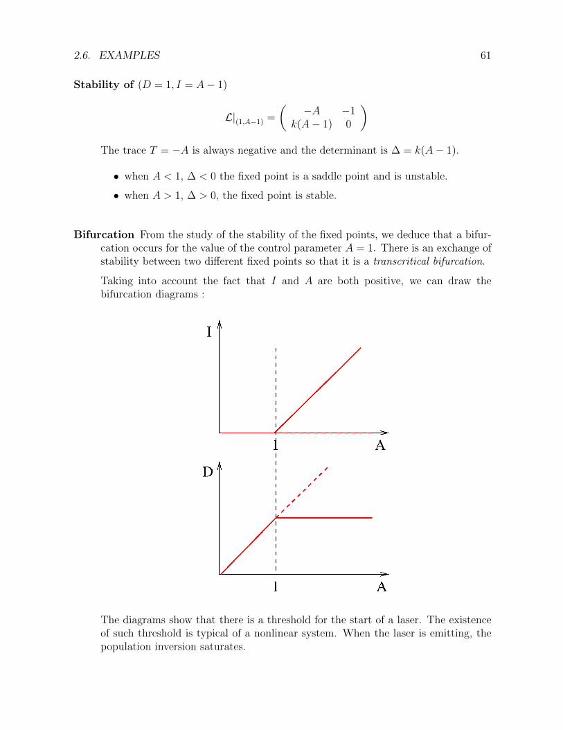
Bifurcation From the study of the stability of the fixed points, we deduce that a bifur-cation occurs for the value of the control parameter A = 1. There is an exchange ofstability between two different fixed points so that it is a transcritical bifurcation.

Taking into account the fact that I and A are both positive, we can draw thebifurcation diagrams :

The diagrams show that there is a threshold for the start of a laser. The existenceof such threshold is typical of a nonlinear system. When the laser is emitting, thepopulation inversion saturates.


2.6.2 Oscillating chemical reactions

2.6.2.a Chemical kinetics

Bibliography: Instabilites, Chaos et Turbulence, P. Manneville.

Let’s consider the elementary step of a chemical reaction :

N∑i=1

niAi →N∑i=1

n′iAi

where the Ai are the N chemical species implied in the reaction (either reactants or prod-ucts), of concentration [Ai], ni (resp. n′i) is the number of mole of Ai before (resp. after)the reaction and can be 0.

The reaction rate is proportional to the number of reactional collisions per unit of time.A reactional collision implies all the reactants at a same location. The probability to haveone species Ai at a given location is proportional to its concentration. Consequently, thereaction rate is of the form k

∏ni=1[Ai]

ni with k the reaction rate constant (which dependson the temperature). When a collision happen, n′i moles of Ai are producted and nimoles consumed, leading to a variation n′i − ni of the number of mole of the species Ai.Consequently, the dynamics of the reaction is given by the N equations :

d[Ai]

dt= (n′i − ni)k

n∏i=1

[Ai]ni

If there are several steps to the reaction, the total variation of [Ai] is given by the sum ofthe variations corresponding to each individual reaction step.

2.6.2.b Belousov-Zhabotinsky oscillating reaction

Bibliography: L’ordre dans le chaos, P. Berge, Y. Pomeau, C. Vidal.

B. Belousov was a Russian chemist who discovered the existence of oscillating chemicalreactions. Such reactions have been studied more deeply afterwards by A. Zhabotinskyin the 60s.

Reactants are1 : sulfuric acid H2SO4, malonic acid CH2(COOH)2, sodium bromateNaBrO3 and cerium sulfate Ce2(SO4)3. Those reactants, in aqueous solution with certainconcentrations, can lead to oscillations in the concentrations of some ions implied in thereaction. Those oscillations can be visualized using a colored redox indicator (e.g. ferroin).

If the reaction is done by simply mixing a given quantity of reactants in a closedcontainer, the oscillations are transitory. To maintain the reaction, you have to supplycontinuously some reactants, to stir continuously the solution and to have an outlet for

1There are several variants of the reaction.

2.6. EXAMPLES 63

the overflow.

The dynamical variables of the system are the instantaneous values of the concentra-tion of all the species in the reactor. But in that kind of experiment only a few variablesare practically measurable. It can be (see L’ordre dans le chaos) :

• the electrical potential difference between two electrodes immersed in the solution.The relationship between the measured voltage and the concentration in Br− (inthe case of the reaction described previously) is given by the Nernst equation.

• the transmission of light through the tank at a given wavelength. The Beer-Lambertlaw is then used to describe the absorption of the light. For example, for λ = 340 nm,the absorption is mainly due to the Ce4+ ions.

Another concern is the parameters which can be tuned in such a system. It can bethe temperature, which will change the constants of the reactions kj, or the concentrationof the species in input, or the flux rates of the pumps that provide the reactants whichchanges the time spent by the reactants in the tank.

Concerning the modeling of the experiment, the problem is that such reactions arevery complicated and can imply a lot of elementary steps which are not known. In fact thecomplete reaction schematics of some of those reactions is still debated. Among the tipsthat help for the modeling of such complicated systems is the fact that the characteristictimes of the steps of the reaction can be very different so that for example the faster onescan be considered to be instantaneous. Using that kind of approximation it is possible toconsider simplier models with a reduce number of differential equations containing onlythe dynamics of interest for the phenomenon studied.

2.6.2.c The Bruxellator

Bibliography:

• Nonlinear dynamics and chaos, S. Strogatz,

• Instabilites, Chaos et Turbulence, P. Manneville

From a theoretical point of view, because of the complexity of real chemical reactions,an approach consists in the search of minimal models which will lead to an oscillatingdynamics. The “Bruxellator” is such a kinetical model proposed by I. Prigogine andR. Lefever in 1968. They considered the global reaction

A+B → C +D


constituted of four steps of elementary reactions and implying two free intermediatesspecies X and Y . The sequence of elementary reactions considered is:

A → X

B +X → Y + C

2X + Y → 3X

X → D

The control parameters of the system are the concentration of species A and B and wesuppose that those concentrations can be maintained at constant values by a continuoussupply. All the reaction constant rates are supposed equal to 1. We note [A] = A.

The kinetics laws give us the following system of differential equations :

dX

dt= (1− 0)A+ (0− 1)BX + (3− 2)X2Y + (0− 1)X

dY

dt= (1− 0)BX + (0− 1)X2Y

dC

dt= (1− 0)BX

dD

dt= (1− 0)X

Note that C and D are directly given by X so that there are finally only two pertinentvariables for the understanding of the dynamics of the system: X and Y . Consequently,we want to study the dynamical system:

dX

dt= A− (B + 1)X +X2Y

dY

dt= BX −X2Y

Fixed points. They are given by :

A = [(B + 1)−XY ]X

BX = X2Y

For A > 0, we have necessarily X 6= 0. We deduce that the only fixed point has forcoordinates in the phase space :

X = A and Y =B

A.

2.6. EXAMPLES 65

Jacobian matrix.

L =

(−(B + 1) + 2XY X2

B − 2XY −X2

)Stability of the fixed point.

L|(A,BA

) =

(B − 1 A2

−B −A2

)

The determinant of the jacobian matrix is ∆ = A2 > 0, and the trace is T =B − 1 − A2. When B < 1 + A2, the fixed point is stable, when B > 1 + A2, it isunstable. At the bifurcation, the fixed point shifts from a stable spiral point to anunstable spiral point.

Consequently, if the concentration A is constant, for low concentration of B, thereaction will reach a stationary state: the concentration of C and D are constantafter a transient. When increasing B, there is a destabilisation of this state througha Hopf bifurcation leading to a limit cycle. The concentrations in C and D thendisplay oscillations.

Poincare-Bendixson. We want to apply the Poincare-Bendixson theorem for given val-ues of A and B with B > 1 + A2.

We search the nullclines, i.e. the two curves along which the vector field is parallelto one of the axis of the phase plane.

• The first curve is given by A− (B + 1)X +X2Y = 0, which leads to:

Y = f(X) =(B + 1)X − A

X2.

To study this function, we compute its derivative: f ′(x) = −(B+1)X2+2AX3 , which

changes of sign when X = 2AB+1

:

X 0 2AB+1

+∞f ′ + 0 -f ↗ ↘

• The second function is given by BX −X2Y = 0, leading to:

Y = g(X) =B

X.


To draw the curves, we need to know the position of the fixed point (which is theintersection of the two nullclines) compared to the maximum of f(X). When thefixed point is unstable:

B > A2 + 1

B + 1 > 2

1 >2

B + 1

A >2A

B + 1

The two curves can then be drawn:

To find a domain on the frontier of which the vector field always points inside thedomain, we need to find a line of negative slope smaller than the one of the vectorfield in the case Y < 0 and X > 0.

dY

dX=

BX −X2Y

A− (B + 1)X +X2Y

= −1 +A−X

A− (B + 1)X +X2Y

when X > A, we thus have dYdX

< −1 so that any line of negative slope strictly largerthan -1 will do, here we used a −1/2 slope:

2.6. EXAMPLES 67

Integration with Matlab We can also for given values of the parameter draw the null-clines (f in cyan and g in green), the vetor field (in blue, rescaled) and an exampleof trajectory (in red, after a transient the trajectory settle on the limit cycle):

Figure 2.12: Integration of the system for A = 1 and B = 3 superimposed with the nullclines and the generaldirections of the vector field (the size of the vectors have been rescaled).


Conclusion

We have presented in this chapter several bifurcations, which correspond to the modifica-tion of the number and/or the nature of the attractors of a dynamical system.

We have illustrated some of those bifurcation by few examples coming from differentfield (start of a laser, chemical reactions).

Bibliography

• In English:

– Nonlinear dynamics and chaos, S. Strogatz

• In French:

– L’ordre dans le chaos, P. Berge, Y. Pomeau, C. Vidal

– Cours DEA de V. Croquette, http://www.phys.ens.fr/cours/notes-de-cours/croquette/index.html

– Dynamiques complexes et morphogenese, C. Misbah

– Les lasers, D. Dangoisse, D. Hennequin, V. Zehnle

– Instabilites, Chaos et Turbulence, P. Manneville

http://www.phys.ens.fr/cours/notes-de-cours/croquette/index.html

http://www.phys.ens.fr/cours/notes-de-cours/croquette/index.html

chapter 2 bifurcations -...

Documents