chapter 17: residential behavior evaluation protocol · demand, including reasonable ... • maggie...
TRANSCRIPT

NREL is a national laboratory of the U.S. Department of Energy Office of Energy Efficiency & Renewable Energy Operated by the Alliance for Sustainable Energy, LLC
This report is available at no cost from the National Renewable Energy Laboratory (NREL) at www.nrel.gov/publications.
Contract No. DE-AC36-08GO28308
Chapter 17: Residential Behavior Evaluation Protocol The Uniform Methods Project: Methods for Determining Energy Efficiency Savings for Specific Measures Created as part of subcontract with period of performance September 2011 – December 2017
This version supersedes the version originally published in January 2015. The content in this version has been updated.
James Stewart Cadmus Waltham, Massachusetts
Annika Todd Lawrence Berkeley National Laboratory Berkeley, California
NREL Technical Monitor: Charles Kurnik
Subcontract Report NREL/SR-7A40-68573 October 2017
NREL is a national laboratory of the U.S. Department of Energy Office of Energy Efficiency & Renewable Energy Operated by the Alliance for Sustainable Energy, LLC
This report is available at no cost from the National Renewable Energy Laboratory (NREL) at www.nrel.gov/publications.
Contract No. DE-AC36-08GO28308
National Renewable Energy Laboratory 15013 Denver West Parkway Golden, CO 80401 303-275-3000 • www.nrel.gov
Chapter 17: Residential Behavior Evaluation Protocol The Uniform Methods Project: Methods for Determining Energy Efficiency Savings for Specific Measures Created as part of subcontract with period of performance September 2011 – December 2017 This version supersedes the version originally published in January 2015. The content in this version has been updated.
James Stewart Cadmus Waltham, Massachusetts
Annika Todd Lawrence Berkeley National Laboratory Berkeley, California
NREL Technical Monitor: Charles Kurnik
Prepared under Subcontract No. LGJ-1-11965-01
Subcontract Report NREL/SR-7A40-68573 October 2017

This publication was reproduced from the best available copy submitted by the subcontractor.
NOTICE
This report was prepared as an account of work sponsored by an agency of the United States government. Neither the United States government nor any agency thereof, nor any of their employees, makes any warranty, express or implied, or assumes any legal liability or responsibility for the accuracy, completeness, or usefulness of any information, apparatus, product, or process disclosed, or represents that its use would not infringe privately owned rights. Reference herein to any specific commercial product, process, or service by trade name, trademark, manufacturer, or otherwise does not necessarily constitute or imply its endorsement, recommendation, or favoring by the United States government or any agency thereof. The views and opinions of authors expressed herein do not necessarily state or reflect those of the United States government or any agency thereof.
This report is available at no cost from the National Renewable Energy Laboratory (NREL) at www.nrel.gov/publications.
Available electronically at SciTech Connect http:/www.osti.gov/scitech
Available for a processing fee to U.S. Department of Energy and its contractors, in paper, from:
U.S. Department of Energy Office of Scientific and Technical Information P.O. Box 62 Oak Ridge, TN 37831-0062 OSTI http://www.osti.gov Phone: 865.576.8401 Fax: 865.576.5728 Email: [email protected]
Available for sale to the public, in paper, from:
U.S. Department of Commerce National Technical Information Service 5301 Shawnee Road Alexandria, VA 22312 NTIS http://www.ntis.gov Phone: 800.553.6847 or 703.605.6000 Fax: 703.605.6900 Email: [email protected]
Cover Photos by Dennis Schroeder: (left to right) NREL 26173, NREL 18302, NREL 19758, NREL 29642, NREL 19795.
NREL prints on paper that contains recycled content.

iii This report is available at no cost from the National Renewable Energy Laboratory (NREL) at www.nrel.gov/publications.
Disclaimer These methods, processes, or best practices (“Practices”) are provided by the National Renewable Energy Laboratory (“NREL”), which is operated by the Alliance for Sustainable Energy LLC (“Alliance”) for the U.S. Department of Energy (the “DOE”).
It is recognized that disclosure of these Practices is provided under the following conditions and warnings: (1) these Practices have been prepared for reference purposes only; (2) these Practices consist of or are based on estimates or assumptions made on a best-efforts basis, based upon present expectations; and (3) these Practices were prepared with existing information and are subject to change without notice.
The user understands that DOE/NREL/ALLIANCE are not obligated to provide the user with any support, consulting, training or assistance of any kind with regard to the use of the Practices or to provide the user with any updates, revisions or new versions thereof. DOE, NREL, and ALLIANCE do not guarantee or endorse any results generated by use of the Practices, and user is entirely responsible for the results and any reliance on the results or the Practices in general.
USER AGREES TO INDEMNIFY DOE/NREL/ALLIANCE AND ITS SUBSIDIARIES, AFFILIATES, OFFICERS, AGENTS, AND EMPLOYEES AGAINST ANY CLAIM OR DEMAND, INCLUDING REASONABLE ATTORNEYS' FEES, RELATED TO USER’S USE OF THE PRACTICES. THE PRACTICES ARE PROVIDED BY DOE/NREL/ALLIANCE "AS IS," AND ANY EXPRESS OR IMPLIED WARRANTIES, INCLUDING BUT NOT LIMITED TO THE IMPLIED WARRANTIES OF MERCHANTABILITY AND FITNESS FOR A PARTICULAR PURPOSE ARE DISCLAIMED. IN NO EVENT SHALL DOE/NREL/ALLIANCE BE LIABLE FOR ANY SPECIAL, INDIRECT OR CONSEQUENTIAL DAMAGES OR ANY DAMAGES WHATSOEVER, INCLUDING BUT NOT LIMITED TO CLAIMS ASSOCIATED WITH THE LOSS OF PROFITS, THAT MAY RESULT FROM AN ACTION IN CONTRACT, NEGLIGENCE OR OTHER TORTIOUS CLAIM THAT ARISES OUT OF OR IN CONNECTION WITH THE ACCESS, USE OR PERFORMANCE OF THE PRACTICES.

iv This report is available at no cost from the National Renewable Energy Laboratory (NREL) at www.nrel.gov/publications.
Preface This document was developed for the U.S. Department of Energy Uniform Methods Project (UMP). The UMP provides model protocols for determining energy and demand savings that result from specific energy-efficiency measures implemented through state and utility programs. In most cases, the measure protocols are based on a particular option identified by the International Performance Verification and Measurement Protocol; however, this work provides a more detailed approach to implementing that option. Each chapter is written by technical experts in collaboration with their peers, reviewed by industry experts, and subject to public review and comment. The protocols are updated on an as-needed basis.
The UMP protocols can be used by utilities, program administrators, public utility commissions, evaluators, and other stakeholders for both program planning and evaluation.
To learn more about the UMP, visit the website, https://energy.gov/eere/about-us/ump-home, or download the UMP introduction document at http://www.nrel.gov/docs/fy17osti/68557.pdf.

v This report is available at no cost from the National Renewable Energy Laboratory (NREL) at www.nrel.gov/publications.
Acknowledgments The chapter authors wish to thank and acknowledge the following individuals for their thoughtful comments and suggestions on drafts of this protocol:
• Ingo Bensch of Evergreen Economics
• Debbie Brannan, Bill Provencher, Kevin Cooney, Carly Olig, and Frank Stern of Navigant
• Cheryl Jenkins of Vermont Energy Investment Corporation
• M. Sami Khawaja of Cadmus
• Maggie McCarey, Marisa Uchin, and Alessandro Orfei of Oracle Utilities (Opower)
• Tim Guiterman and John Backus Mayes of Energy Savvy
• Julie Michals of 4TheFuture.
Suggested Citation Stewart, J.; Todd, A. (2017). Chapter 17: Residential Behavior Protocol, The Uniform Methods Project: Methods for Determining Energy-Efficiency Savings for Specific Measures. Golden, CO; National Renewable Energy Laboratory. NREL/SR-7A40-68573. http://www.nrel.gov/docs/fy17osti/68573.pdf

vi This report is available at no cost from the National Renewable Energy Laboratory (NREL) at www.nrel.gov/publications.
Acronyms BB behavior-based
DiD
IPMVP
difference-in-differences
International Performance Measurement and Verification Protocol
ITT intent-to-treat
IV instrumental variable
LATE local average treatment effect
OLS
PG&E
ordinary least squares
Pacific Gas & Electric
RCT randomized control trial
RED randomized encouragement design
SEE Action State and Local Energy Efficiency Action
TOT
UMP
treatment effect on the treated
Uniform Methods Project

vii This report is available at no cost from the National Renewable Energy Laboratory (NREL) at www.nrel.gov/publications.
Protocol Updates The original version of this protocol was published in January 2015. The authors updated the protocol by making the following changes:
• Incorporated findings from recent research comparing the accuracy of savings estimates from randomized experiments and quasi-experiments
• Presented new developments in the estimation of energy savings from behavior-based programs, including the post-period only model with pre-period controls (Allcott 2014)
• Updated the discussion of randomized encouragement designs to emphasize the importance of having large sample sizes or a sufficient proportion of compliers as well as the application of instrumental variables two-stage least squares for obtaining estimates of the local average treatment effect
• Incorporated new research regarding the calculation of statistical power and sizing of analysis samples
• Provided more guidance about estimating impacts of behavior-based programs on participation in other energy efficiency programs
• Edited the text in various places to improve organization or to clarify concepts and recommendations.

viii This report is available at no cost from the National Renewable Energy Laboratory (NREL) at www.nrel.gov/publications.
Table of Contents 1 Measure Description ............................................................................................................................ 1 2 Application Conditions of Protocol .................................................................................................... 2
2.1 Examples of Protocol Applicability .............................................................................................. 3 3 Savings Concepts................................................................................................................................. 5
3.1 Definitions ..................................................................................................................................... 5 3.2 Randomized Experimental Research Designs ............................................................................... 6 3.3 Basic Features ............................................................................................................................... 7
3.3.1 Common Features of Randomized Control Trial Designs ............................................... 7 3.4 Common Designs .......................................................................................................................... 9
3.4.1 Randomized Control Trial With Opt-Out Program Design ............................................. 9 3.4.2 Randomized Control Trial With Opt-In Program Design .............................................. 10 3.4.3 Randomized Encouragement Design ............................................................................. 12 3.4.4 Persistence Design.......................................................................................................... 14
3.5 Evaluation Benefits and Implementation Requirements of Randomized Experiments .............. 15 4 Savings Estimation ............................................................................................................................ 18
4.1 IPMVP Option............................................................................................................................. 19 4.2 Sample Design............................................................................................................................. 19
4.2.1 Sample Size .................................................................................................................... 19 4.2.2 Random Assignment to Treatment and Control Groups by Independent Third Party ... 21 4.2.3 Equivalency Check ......................................................................................................... 21
4.3 Data Requirements and Collection .............................................................................................. 22 4.3.1 Energy Use Data............................................................................................................. 22 4.3.2 Makeup of Analysis Sample .......................................................................................... 23 4.3.3 Other Data Requirements ............................................................................................... 23 4.3.4 Data Collection Method ................................................................................................. 24
4.4 Analysis Methods ........................................................................................................................ 24 4.4.1 Panel Regression Analysis ............................................................................................. 24 4.4.2 Panel Regression Model Specifications ......................................................................... 25 4.4.3 Simple Differences Regression Model of Energy Use ................................................... 25 4.4.4 Simple Differences Regression Estimate of Heterogeneous Savings Impacts ............... 26 4.4.5 Simple Differences Regression Estimate of Savings During Each Time Period ........... 27 4.4.6 Difference-in-Differences Regression Model of Energy Use ........................................ 28 4.4.7 DiD Estimate of Savings for Each Time Period ............................................................. 29 4.4.8 Simple Differences Regression Model with Pre-Treatment Energy Consumption ........ 30 4.4.9 Randomized Encouragement Design ............................................................................. 32 4.4.10 Models for Estimating Savings Persistence ................................................................... 33 4.4.11 Standard Errors ............................................................................................................... 34 4.4.12 Opt-Out Subjects and Account Closures ........................................................................ 35
4.5 Energy Efficiency Program Uplift and Double Counting of Savings ......................................... 36 5 Reporting ............................................................................................................................................. 39 6 Looking Forward................................................................................................................................. 40 7 References .......................................................................................................................................... 41

ix This report is available at no cost from the National Renewable Energy Laboratory (NREL) at www.nrel.gov/publications.
List of Figures Figure 1. Illustration of RCT with opt-out program design .......................................................................... 9 Figure 2. Illustration of RCT with opt-in program design .......................................................................... 11 Figure 3. Illustration of RED program design ............................................................................................ 13 Figure 4. Example of DiD regression savings estimates ............................................................................. 30 Figure 5. Calculation of double-counted savings ........................................................................................ 37
List of Tables Table 1. Benefits and Implementation Requirements of Randomized Experiments .................................. 16 Table 2. Considerations in Selecting a Randomized Experimental Design ................................................ 17

1 This report is available at no cost from the National Renewable Energy Laboratory (NREL) at www.nrel.gov/publications.
1 Measure Description Residential behavior-based (BB) programs use strategies grounded in the behavioral and social sciences to influence household energy use. These may include providing households with real-time or delayed feedback about their energy use; supplying energy efficiency education and tips; rewarding households for reducing their energy use; comparing households to their peers; and establishing games, tournaments, and competitions.1 BB programs often target multiple energy end uses and encourage energy savings, demand savings, or both. Savings from BB programs are usually a small percentage of energy use, typically less than 5%.2
Utilities introduced the first large-scale residential BB programs in 2008. Since then, dozens of utilities have offered these programs to their customers.3 Although program designs differ, many share these features:
• They are implemented as randomized experiments wherein eligible homes are randomly assigned to treatment or control groups.
• They are large scale by energy efficiency program standards, targeting thousands of utility customers.
• They provide customers with analyses of their historical consumption, energy savings tips, and energy efficiency comparisons to neighboring homes, either in personalized home reports or through a web portal, or offer incentives for savings energy.
• They are typically implemented by outside vendors.4 Utilities will continue to implement residential BB programs as large-scale, randomized control trials (RCTs); however, some are now experimenting with alternative program designs that are smaller scale; involve new communication channels such as the web, social media, and text messaging; or that employ novel strategies for encouraging behavior change (for example, Facebook competitions).5 These programs will create new evaluation challenges and may require different evaluation methods than those currently employed to verify any savings they generate. Quasi-experimental methods, however, require stronger assumptions to yield valid savings estimates and may not measure savings with the same degree of validity and accuracy as randomized experiments.
1 See Ignelzi et al. (2013) for a classification and descriptions of different BB intervention strategies and Mazur-Stommen and Farley (2013) for a survey and classification of current BB programs. Also, a Minnesota Department of Commerce, Division of Energy Resources white paper (2015) defines, classifies, and benchmarks behavioral intervention strategies. 2 See Allcott (2011), Davis (2011), and Rosenberg et al. (2013) for savings estimates from residential BB programs. 3 See the 2013 Consortium for Energy Efficiency (CEE) database for a list of utility behavior programs; it is available for download: http://library.cee1.org/content/2013-behavior-program-summary-public-version. 4 Vendors that offer residential BB programs include Aclara, C3 Energy, ICF, Oracle Utilities (Opower), Simple Energy, and Tendril. 5 The 2013 CEE database includes descriptions of many residential BB programs with alternative designs such community-focused programs, college dormitory programs, K-12 school programs, and programs relying on social media.

2 This report is available at no cost from the National Renewable Energy Laboratory (NREL) at www.nrel.gov/publications.
2 Application Conditions of Protocol This protocol recommends the use of RCTs or randomized encouragement designs (REDs) for estimating savings from BB programs. A significant body of research indicates that randomized experiments result in unbiased and robust estimates of program energy and demand savings. Moreover, recently evaluators have conducted studies comparing the accuracy of savings estimates from randomized experiments and quasi-experiments or observational studies. These comparisons suggest that randomized experiments produce the most accurate savings estimates.6
This protocol applies to BB programs that satisfy the following conditions:7
• Residential utility customers are the target.
• Energy or demand savings are the objective.
• An appropriately sized analysis sample can be constructed.
• Treated customers can be identified and accurate energy use measurements for sampled units are available.
• It must be possible to isolate the treatment effect when measuring savings. This protocol applies only to residential BB programs. Although the number of nonresidential BB programs is growing, utilities offer a larger number of residential BB programs and to a much larger number of residential customers.8 As evaluators accumulate more experience, the National Renewable Energy Laboratory (NREL) could expand this protocol to cover nonresidential programs to which similar evaluation methods are applicable.
This protocol also addresses best practices for estimating energy and demand savings. There are no significant conceptual differences between measuring energy savings and measuring demand savings when interval data are available; thus, evaluators can apply the algorithms in this protocol for calculating BB program savings to either. The protocol does not directly address the evaluation of other BB program objectives, such as increasing utility customer satisfaction, educating customers about their energy use, or increasing awareness of energy efficiency.9 But
6 Allcott (2011) compares RCT difference-in-differences (DiD) savings estimates with quasi-experimental simple differences and DiD savings estimates for several home energy reports programs. He found large differences between the RCT and quasi-experimental estimates. Also, Baylis et al. (2016) analyzed data from a California utility time-of-use and critical peak pricing pilot program and found that RCT produced more accurate savings estimates than quasi-experimental methods such as DiD and propensity score matching that relied on partly random but uncontrolled variation in participation. 7 As discussed in the “Considering Resource Constraints” section of the UMP Chapter 1: Introduction, small utilities (as defined under U.S. Small Business Administration regulations) may face additional constraints in undertaking this protocol. Therefore, alternative methodologies should be considered for such utilities. 8 Evaluators may be able to apply the methods recommended in this protocol to the evaluation of some nonresidential BB programs. For example, Pacific Gas and Electric (PG&E) offers a Business Energy Reports Program, which it implemented as an RCT (Seelig 2013). Also, Xcel Energy implemented a business energy reports program as an RCT (Stewart 2013b). Other nonresidential BB programs may not lend themselves to evaluation by randomized experiment. For example, many strategic energy management programs enroll large industrial customers with unique production and energy consumption characteristics for which a randomized experiment would not be feasible (NREL 2017). 9 Process evaluation objectives may be important, and omission of them from this protocol should not be interpreted as a statement that these objectives should not be considered by program administrators.

3 This report is available at no cost from the National Renewable Energy Laboratory (NREL) at www.nrel.gov/publications.
these program outcomes could be studied in a complementary fashion alongside the energy savings.
This protocol also requires that the analysis sample be large enough to detect the expected savings with a high degree of confidence. Because most BB programs result in small percentage savings, a large sample size is required to detect savings. This protocol does not address evaluations of BB programs with a small number of participants.
Finally, this protocol requires that the energy use of participants or households affected by the program (for the treatment and control groups) can be clearly identified and measured. Typically, the analysis unit is the household; in this case, treatment group households must be identifiable and individual household energy use must be measurable. However, depending on the BB program, the analysis units may not be households. For example, for a BB program that generates an energy competition between hundreds of housing floors at a university, the analysis unit may be floors; in this case, the energy use measurement of individual floors must be available.
The characteristics of BB programs that do not determine the applicability of the evaluation protocol include:
• Whether the program is opt-in or opt-out10
• The specific behavior-modification theory or strategy
• The channel(s) through which program information is communicated. Although this protocol strongly recommends RCTs or REDs, it also recognizes that implementing these methods may not always be feasible. Government regulations or program designs may prevent the utilization of randomized experiments for evaluating BB programs. In these cases, evaluators must employ quasi-experimental methods, which require stronger assumptions than do randomized experiments to yield valid savings estimates.11 If these assumptions are violated, quasi-experimental methods may produce biased results. The extent of the biases in the estimates is not knowable ex ante, so results will be less reliable. Because there is currently not enough evidence of quasi-experimental methods that perform well, this protocol refrains from recommending non-RCT evaluation methods. As noted above, studies have found quasi-experiments produce less accurate savings estimates than randomized experiments. A good reference for applying quasi-experimental methods to BB program evaluation is State and Local Energy Efficiency Action (SEE Action) (2012) or Cappers et al. (2013). As more evidence accumulates about the efficacy of quasi-experiments, the National Renewable Energy Laboratory may update this protocol as appropriate.
2.1 Examples of Protocol Applicability Examples of residential BB programs for which the evaluation protocol applies follow: 10 In opt-in programs, customers enroll or select to participate. In opt-out programs, the utility enrolls the customers, and the customers remain in the program until they opt out. An example opt-in program is having a utility web portal with home energy use information and energy efficiency tips that residential customers can use if they choose. An example opt-out program is sending energy reports to utility selected customers. 11 For example, Harding and Hsiaw (2012) use variation in timing of adoption of an online goal-setting tool to estimate savings from the tool.

4 This report is available at no cost from the National Renewable Energy Laboratory (NREL) at www.nrel.gov/publications.
• Example 1: A utility sends energy reports encouraging conservation steps to thousands of randomly selected residential customers.
• Example 2: Several hundred residential customers enroll in a Wi-Fi-enabled thermostat pilot program offered by the utility.
• Example 3: A utility invites thousands of residential customers to use its web portal to track their energy use in real time, set goals for energy saving, find ideas about how to reduce their energy use, and receive points or rewards for saving energy.
• Example 4: A utility sends voice, text, and email messages to thousands of residential utility customers encouraging—and providing tips for— reducing energy use during an impending peak demand event.
Examples of programs for which the protocol does not apply follow:
• Example 5: A utility uses a mass-media advertising campaign that relies on radio and other broadcast media to encourage residential customers to conserve energy.
• Example 6: A utility initiates a social media campaign (for example, using Facebook or Twitter) to encourage energy conservation.
• Example 7: A utility runs a pilot program to test the savings from in-home energy-use displays, and enrolls too few customers to detect the expected savings.
• Example 8: A utility runs a BB program in a large college dormitory to change student attitudes about energy use. The utility randomly assigns some rooms to the treatment group. The dorm is master-metered.
The protocol does not apply to Example 5 or Example 6 because the evaluator cannot identify who received the messages. The protocol does not apply to Example 7 because too few customers are in the pilot to accurately detect energy savings. The protocol does not apply to Example 8 because energy-use data are not available for the specific rooms in the treatment and control groups.

5 This report is available at no cost from the National Renewable Energy Laboratory (NREL) at www.nrel.gov/publications.
3 Savings Concepts The protocol recommends RCTs and REDs to develop unbiased and robust estimates of energy or demand savings from BB programs that satisfy the applicability conditions described in Section 2. Unless otherwise noted, all references in this protocol to savings are to net savings.
Section 3.1 defines some key concepts and Section 3.2 describes specific evaluation methods.
3.1 Definitions The following key concepts are used throughout this protocol.
Control group. In an experiment, the control group comprises subjects (for example, utility customers) who do not receive the program intervention or treatment.
Experimental design.12 Randomized experimental designs rely on observing the energy use of subjects who were randomly assigned to program treatments or interventions in a controlled process.
External validity. Savings estimates are externally valid if evaluators can apply them to different populations or different time periods from those studied.
Internal validity. Savings estimates are internally valid if the savings estimator is expected to equal the causal effect of the program on consumption.
Opt-in program. Utilities use opt-in BB programs if the customers must agree to participate, and the utility cannot administer treatment without consent.
Opt-out program. Utilities use opt-out BB programs if customers need not agree to participate. The utility can administer treatment without consent, and customers remain enrolled until they ask the utility to stop the treatment.
Quasi-experimental design. Quasi-experimental designs rely on a comparison group who is not obtained via random assignment. Such designs observe energy use and determine program treatments or interventions based on factors that may be partly random but not controlled.
Randomized Control Trial (RCT). An RCT uses random variation in which subjects are exposed to the program treatment to obtain an estimate of the treatment effect. By randomly assigning subjects to treatment, an RCT controls for factors that could confound measurement of the treatment effect. An RCT is expected to yield an unbiased estimate of program savings. Evaluators randomly assign subjects from a study population to a treatment group or a control group. Subjects in a treatment group receive one program treatment (there may be multiple treatments), while subjects in the control group receive no treatment. The RCT ensures that receiving the treatment is uncorrelated with the subjects’ pre-treatment energy use, and that evaluators can attribute any difference in energy use between the groups to the treatment.
12 When this protocol uses the term randomized experiments, it refers to RCTs or REDs, not other experimental evaluation approaches such as natural experiments or quasi-experiments.

6 This report is available at no cost from the National Renewable Energy Laboratory (NREL) at www.nrel.gov/publications.
Randomized Encouragement Design (RED). In an RED, evaluators randomly assign subjects to a treatment group that receives encouragement to participate in a program or to a control group who does not receive encouragement. The RED yields an unbiased estimate of the effect on energy use of encouraging energy-efficient behaviors and the effect on customers who participate because of the encouragement.
Treatment. A treatment is an intervention administered through the BB program to subjects in the treatment group. Depending on the research design, the treatment may be a program intervention or encouragement to accept an intervention.
Treatment effect. This is the effect of the BB program intervention(s) on energy use for a specific population and time period.
Treatment group. The treatment group includes subjects who receive the treatment.
3.2 Randomized Experimental Research Designs This section outlines the application of randomized experiments for evaluating BB programs. The most important benefit of an RCT or RED is that, if carried out correctly, the experiment results in an unbiased estimate of the program’s causal impact.13 Unbiased savings estimates have internal validity. A result is internally valid if the evaluator can expect the value of the estimator to equal the savings caused by the program intervention. The principal threat to internal validity in BB program evaluation derives from potential selection bias about who receives a program intervention. RCTs and REDs yield unbiased savings estimates because they ensure that receiving the program intervention is uncorrelated with the subjects’ energy use.
Randomized experiments may yield savings estimates that are applicable to other populations or time periods, making them externally valid. Whether savings have external validity will depend on the specific research design, the study population, and other program features.14 Program administrators should exercise caution in applying BB program savings estimates for one population to another or to the same population at a later time, since differences in population characteristics, weather, or naturally-occurring efficiency can cause savings to change.
A benefit of field experiments is their versatility: evaluators can apply them to a wide range of BB programs regardless of whether they are opt-in or opt-out programs. Evaluators can apply randomized experiments to any program where the objective is to achieve energy or demand savings; evaluators can construct an appropriately sized analysis sample; and accurate measurements of the energy use of sampled units are available.
Randomized experiments generally yield highly robust savings estimates that are not model dependent; that is, they do not depend on the specification of the model used for estimation.
The choice of whether to use an RCT or RED to evaluate program savings should depend on several factors, including whether it is an opt-in or opt-out program, the expected number of
13 List (2011) describes many of the benefits of employing randomized field experiments. 14 Allcott (2015) analyzes the external validity of savings estimates from evaluations of 111 RCTs of home energy reports programs in the United States and shows that the first utilities implementing the programs achieved higher savings than utilities that implemented such programs subsequently.

7 This report is available at no cost from the National Renewable Energy Laboratory (NREL) at www.nrel.gov/publications.
program participants, and the utility’s tolerance for subjecting customers to the requirements of an experiment. For example, using an RCT for an opt-in program might require delaying or denying participation for some customers. A utility may prefer to use an RED to accommodate all the customers who want to participate.
Implementing an RCT or RED design requires upfront planning. Program evaluation must be an integral part of the program planning process, which is evident in the randomized experiment research design descriptions in Section 3.3.
3.3 Basic Features This section outlines several types of RCT research designs, which are simple but extremely powerful research tools. The core feature of RCT is the random assignment of study subjects (for example, utility customers, floors of a college dormitory) to a treatment group that receives or experiences an intervention or to a control group that does not receive the intervention.
Section 3.3.1 outlines some common features of RCTs and discusses specific cases.
3.3.1 Common Features of Randomized Control Trial Designs The key requirements of an RCT are incorporated into the following steps:
1. Identify the study population: The program administrator screens the utility population if the program intervention is offered to certain customer segments only, such as single-family homes. Programs designers can base eligibility on dwelling type (for example, single family, multifamily), geographic location, completeness of recent billing history, heating fuel type, utility rate class, or other energy use characteristics.
2. Determine sample sizes: The numbers of subjects to assign to the treatment and control groups depend on the type of randomized experiment (for example, REDs and opt-out RCTs generally require more customers) and hypothesized savings. The number of subjects assigned to the treatment versus control groups should be large enough to detect the hypothesized program effect with sufficient probability, though it is not necessary for the treatment and control groups to be equally sized.15
Evaluators can use a statistical power analysis to determine the number of subjects required. This results in minimum sample sizes for the treatment and control groups as a function of the hypothesized program effect, the coefficient of variation of energy use, the specific analysis approach that will be used (for example, simple differences of means, a repeated measure analysis where there are multiple observations of energy consumption at different time periods for the same subject [aka, panel analysis]), and tolerances for Type I and Type II statistical errors.16 Most statistical software (including SAS, STATA, and R) now include packages for performing statistical power analyses. It
15 The number of subjects in the treatment group may also depend on the savings goal for the program. 16 A Type I error occurs when a researcher rejects a null hypothesis that is true. Statistical confidence equals 1 minus the probability of a Type I error. A Type II error occurs when a researcher accepts a null hypothesis that is false. Many researchers agree that the probability of a 5% Type I error and a 20% Type II error is acceptable. See List et al. (2010).

8 This report is available at no cost from the National Renewable Energy Laboratory (NREL) at www.nrel.gov/publications.
is not uncommon for BB programs with expected savings of less than 3% to require thousands of subjects in the treatment and control groups.17
An important component of the random assignment process is to verify that the treatment and control groups are statistically equivalent or balanced in their observed covariates. At a minimum, evaluators should check before the intervention for statistically significant differences in average pre-treatment energy use and in the distribution of pre-treatment energy use between treatment and control homes.
3. Randomly assign subjects to treatments and control: Study subjects should be randomly assigned to treatment and control groups. To maximize the credibility and acceptance of BB program evaluations, this protocol recommends that a qualified independent third party perform the random assignment. Also, to preserve the integrity of the experiment, customers must not choose their assignments. The procedure for randomly assigning subjects to treatment and control groups should be transparent and well documented.
4. Administer the treatment: The intervention must be administered to the treatment group and withheld from the control group. To avoid a Hawthorne effect, in which subjects change their energy use in response to observation, control group subjects should receive minimal information about the study. Depending on the research subject and intervention type, the utility may administer treatment once or repeatedly and for different durations. However, the treatment period should be long enough for evaluators to observe any effects of the intervention.
5. Collect data: Data must be collected from all study subjects, not only from those who chose to participate or only from those who participated for the whole study or experiment.
Preferably, evaluators collect multiple pre- and post-treatment energy use measurements. Such data enable the evaluator to control for time-invariant differences in average energy use between the treatment and control groups to obtain more precise savings estimates. Step 6 discusses this in further detail.
6. Estimate savings:18 Evaluators should calculate savings as the difference in energy use or difference-in-differences (DiD) of energy use between the subjects who were initially assigned to the treatment versus the control group. To be able to calculate an unbiased savings estimate, evaluators must compare the energy use from the entire group of subjects who were originally randomly assigned to the treatment group to the entire group of subjects who were originally randomly assigned to the control group. For example, the savings estimate would be biased if evaluators used only data from utility customers in the treatment group who chose to participate in the study.
The difference in energy use between the treatment and control groups, usually called an intent-to-treat (ITT) effect, is an unbiased estimate of savings because subjects were
17 EPRI (2010) illustrates that, all else equal, repeated measure designs, which exploit multiple observations of energy use per subject both before and after program intervention, require smaller analysis sample sizes than other types of designs. 18 This protocol focuses on estimating average treatment effects; however, treatment effects of behavior programs may be heterogeneous. Costa and Kahn (2010) discuss how treatment effects can depend on political ideology and Allcott (2011) discusses how treatment effects can depend on pretreatment energy use.

9 This report is available at no cost from the National Renewable Energy Laboratory (NREL) at www.nrel.gov/publications.
randomly assigned to the treatment and control groups. The effect is an ITT because, in contrast to many randomized clinical medical trials, ensuring that treatment group subjects in most BB programs comply with the treatment is impossible. For example, some households may opt out of an energy reports program, or they may fail to notice or simply ignore the energy reports. Thus, the effect is ITT, and the evaluator should base the results on the initial assignment of subjects to the treatment group, whether or not subjects actually complied with the treatment.
The savings estimation approach should be well documented, transparent, and performed by an independent third party.
3.4 Common Designs This section describes some of the RCT designs commonly used in BB programs.
3.4.1 Randomized Control Trial With Opt-Out Program Design One common type of RCT includes the option for treated subjects to opt out of receiving the program treatment. This design reflects the most realistic description of how most BB programs work. For example, in energy reports programs, some treated customers may ask the utility to stop sending them reports.
Figure 1 depicts the process flow of an RCT in which treated customers can opt out of the program. In this illustration, the utility initially screened utility customers to refine the study population.19
Figure 1. Illustration of RCT with opt-out program design
Customers who pass the screening constitute the study population or sample frame. The savings estimate will apply to this population. Alternatively, the utility may want to study only a sample of the screened population, in which case a third party should sample randomly from the study population. The analysis sample must be large enough to meet the minimum size requirement for
19 This graphic and the following ones are variations of those that appeared in SEE Action (2012). A coauthor of the SEE Action report and the creator of that reports’ figures is one of the authors of this protocol.

10 This report is available at no cost from the National Renewable Energy Laboratory (NREL) at www.nrel.gov/publications.
the treatment and control groups. The program savings goals and desired statistical power will determine the size of the treatment group.
The next steps in an RCT with opt-out program design are to (1) randomly assign subjects in the study population to the program treatment and control groups, (2) administer the program treatments, and (3) collect energy use data.
The distinguishing feature of this randomized experimental design is that customers can opt out of the program. As Figure 1 shows, evaluators should include opt-out subjects in the energy savings analysis to ensure unbiased savings estimates. Evaluators can then calculate savings as the difference in average energy use between treatment group customers, including opt-out subjects and control group customers. Removing opt-out subjects from the analysis would bias the savings estimate because identifying subjects in the control group who would have also opted out had they received the treatment is impossible. The resulting savings estimate is therefore an average of the savings of treated customers who remain in the program and of customers who opted out.
Depending on the type of BB program, the percentage of customers who opt out may be small, and may not affect the savings estimates significantly (for example, few customers generally opt out of energy reports programs).
3.4.2 Randomized Control Trial With Opt-In Program Design Utilities must have consent from customers to administer some program interventions. Examples include web-based home audit or energy consumption tools; programmable, communicating thermostats with wireless capability; online class about energy rates and efficiency; or in-home displays. All these interventions require that customers opt in to the program. These interventions contrast with interventions such as home energy reports that can be administered to subjects without their agreement.
An opt-in RCT (Figure 2) can accommodate the necessity for customers to opt in to some BB programs. This design results in an unbiased estimate of the ITT effect for customers who opt in to the program. The estimate of savings will have internal validity; however, it will not have external validity because it will not apply to subjects who do not opt in.

11 This report is available at no cost from the National Renewable Energy Laboratory (NREL) at www.nrel.gov/publications.
Figure 2. Illustration of RCT with opt-in program design
Implementing opt-in RCTs is very similar to implementing opt-out RCTs. The first step, screening utility customers for eligibility to determine the study population, is the same. The next step is to market the program to eligible customers. Some eligible customers may then agree to participate. Then, an independent third party randomly assigns these customers to either a treatment group that receives the intervention or a control group that does not. The utility delays or denies participation in the program to customers assigned to the control group. Thus, only customers who opted in and were assigned to the treatment group will receive the treatment.
Randomizing only opt-in customers ensures that the treatment and control groups are equivalent in their energy use characteristics. In contrast, other quasi-experimental approaches, such as matching participants to nonparticipants, cannot guarantee either this equivalence or the internal validity of the savings estimates.
After the random assignment, the opt-in RCT proceeds the same as an RCT with opt-out subjects: the utility administers the intervention to the treatment group. The evaluator collects energy use data from the treatment and control groups, then estimates energy savings as the difference in energy use between the groups. The evaluator does not collect energy use data for customers who do not opt in to the program.
An important difference between the opt-in RCTs and RCTs with opt-out subjects is how to interpret the savings estimates. In the RCT with opt-out subjects, the evaluator bases the savings estimate on a comparison of the energy use between treatment and control groups, which pertains to the entire study population. In contrast, in the opt-in RCT, the savings estimate pertains to the subset of customers who opted into the program, and the difference in energy use represents the treatment effect on customers who opted in to the program. Opt-in RCT savings estimates have internal validity; however, they do not apply to customers who did not opt in to the program.

12 This report is available at no cost from the National Renewable Energy Laboratory (NREL) at www.nrel.gov/publications.
3.4.3 Randomized Encouragement Design For some opt-in BB programs, delaying or denying participation to some customers may be undesirable. In this case, neither the opt-out nor the opt-in RCT design would be appropriate, and this protocol recommends an RED. Instead of randomly assigning subjects to receive or not receive an intervention, a third party randomly assigns them to a treatment group that is encouraged to accept the intervention (that is, to participate in a program or adopt a measure), or to a control group that does not receive encouragement. Examples of common kinds of encouragement include direct paper mail or e-mail informing customers about the opportunity to participate in a BB program. Customers who receive the encouragement can refuse to participate, and, depending on the program design, control group customers who learn about the program may be able to participate.
The RED yields an unbiased estimate of the effect of encouragement on energy use and, depending on the program design, can also provide an unbiased estimate of either the effect of the intervention on customers who accept it because of the encouragement or the effect of the intervention on all customers who accept it. A necessary condition for an RED to produce an unbiased estimate of savings from the BB intervention is that the encouragement only affects energy consumption for those customers that take up the BB intervention, and it does not affect the energy consumption for customers who receive the encouragement but do not take up the BB intervention. For example, the RED must be such that customers who receive a direct mailing encouraging them to log into a website with personalized energy efficiency recommendations only save energy if they decide to log into the site; the mailing itself must not cause the customer to save energy if the customer never logs on. If the encouragement causes customers to save energy, it may be impossible to isolate the savings from the intervention. Programs designed as an RED should try to design and distribute encouragement materials that do not affect consumption. If evaluators expect that the encouragement will cause energy savings, they can send the same or similar messaging but without a program enrollment option to the control group or to a second randomized control group. Evaluators could use the second randomized control group to test whether the encouragement produces savings and to estimate the savings from the encouragement.
Figure 3 illustrates the process flow for a program using an RED. As with the RCT with opt-out and opt-in RCT, the first two steps are to identify the sample frame and select a study population. Next, like the RCT with opt out, a third party randomly assigns subjects to a treatment group, which receives encouragement, or to a control group, which does not. For example, a utility might employ a direct mail campaign that encourages treatment group customers to use an online audit tool. The utility would administer the intervention to treatment group customers who opt-in. Although customers in the control group did not receive encouragement, some may learn about the program and decide to sign up. The program design shown in Figure 3 allows for control group customers to receive the behavioral intervention.

13 This report is available at no cost from the National Renewable Energy Laboratory (NREL) at www.nrel.gov/publications.
Figure 3. Illustration of RED program design
In Figure 3, the difference in energy use between homes in the treatment and control groups is an estimate of savings from the encouragement, not from the intervention. However, evaluators can also use the difference in energy use to estimate savings for customers who accept the intervention because of the encouragement. To see this, consider that the study population comprises three types of subjects: (1) always takers, or those who would accept the intervention whether encouraged or not; (2) never takers, or those who would never accept the intervention even if encouraged; and (3) compliers, or those who would accept the intervention only if encouraged. Compliers participate only after receiving the encouragement.
Because eligible subjects are randomly assigned to groups depending on whether they receive encouragement, the treatment and control groups are expected to have equal frequencies of always takers, never takers, and compliers. After treatment, the only difference between the treatment and control groups is that compliers in the treatment group accept the treatment and compliers in the control group do not. In both groups, always takers accept the treatment and never takers always refuse the treatment. Therefore, the difference in energy use between the groups reflects the treatment effect of encouragement on compliers (known as the local average treatment effect [LATE]).
Furthermore, for the study to have enough statistical power to detect the expected effect, there must be very large encouraged and non-encouraged groups relative to an RCT or quasi-experimental design and/or a high proportion of compliers in the treatment group; a power calculation should be done to ensure that there are enough customers in the encouraged and non-encouraged groups to produce significant savings estimates for the expected take-up rate.20
To estimate the effect of the intervention on compliers, evaluators can either employ instrumental variables (IV), using the random assignment of customers to receive encouragement as an instrument for the customer’s decision to accept the intervention (that is, participate). The IV approach is presented in Section 4.3. Another option is that evaluators can scale the treatment effect of the encouragement by the difference between treatment and control groups in the
20 For an example of a power calculation for REDs, see Fowlie (2010).

14 This report is available at no cost from the National Renewable Energy Laboratory (NREL) at www.nrel.gov/publications.
percentage of customers who receive the intervention (note that in this equation, if the non-encouraged customers are not allowed to take up the treatment, the second term in the denominator will be zero):21
1/(% of encouraged customers who accepted – % of non-encouraged customers who accepted)
If customers in the control group are permitted to participate if they find out about the treatment even though they did not receive encouragement, the LATE does not capture the program effect on always takers. (Note, however, in most programs, the control group is not permitted to take up the treatment). If customers in the control group are permitted to participate, the LATE may differ from the average treatment effect unless the savings from the intervention is the same for compliers and always takers. However, the LATE will be equal to the average treatment effect if the control group customers (non-encouraged customers) are not permitted to take up the treatment.
For BB programs with REDs that do not permit control group customers to participate, evaluators can estimate the treatment effect on the treated (TOT). The TOT is the effect of the program intervention on all customers who accept the intervention. In this case, the difference in energy use between the treatment and control groups reflects the impact of the encouragement on the always takers and compliers in the treatment group. Scaling the difference by the inverse of the percentage of customers who accepted the intervention yields an estimate of the TOT impact.22
Successful application of an RED requires that compliers constitute a percentage of the encouraged population that is sufficiently large given the number of encouraged customers.23 If the RED generates too few compliers, the effects of the encouragement and receiving the intervention cannot be precisely estimated. Therefore, before employing an RED, evaluators should ensure that the sample size is sufficiently large and that the encouragement will result in the required number of compliers. If the risk of an RED generating too few compliers is significant, evaluators may want to consider alternative approaches, including quasi-experimental methods.
3.4.4 Persistence Design Studies of home energy reports programs show that program savings persist while homes continue to receive reports. However, utilities and regulators may want to know what happens to BB program savings after the behavioral intervention ends. They may wish to measure whether their savings persist after the utility stops sending reports and for how long, as well as the rate of the savings “decay.” As Allcott and Rodgers (2014) demonstrate, the rate of savings decay after treatment ends has significant implications for the performance of efficiency program portfolios 21 This approach of estimating savings from the intervention because of encouragement assumes zero savings for customers who received encouragement but did not accept the intervention. If encouraged customers who did not accept the intervention reduced their energy use in response to the encouragement, the savings estimate for compliers will be biased upward. 22 If the effect of program participation is the same for compliers as for others, those who would have participated without encouragement (always takers) and those who do not participate (never takers), the RED will yield an unbiased estimate of the population average treatment effect. 23 For an example of the successful application of an RED, see SMUD (2013).

15 This report is available at no cost from the National Renewable Energy Laboratory (NREL) at www.nrel.gov/publications.
and measuring cost effectiveness of BB programs. Initial studies of home energy reports programs indicate that some portion of savings may persist after the treatment stops, although further research is needed.24
This protocol recommends that evaluators employ RCTs to estimate the persistence of BB program savings after participants stop receiving the intervention. The application of an RCT to a savings persistence study proceeds similarly to the application of RCTs previously discussed.
The utility is assumed to implement the BB program as an RCT with opt-out design; that is, customers from the study population were randomly assigned to a treatment group that received an intervention or to a control group that did not. Customers are able to opt out of the program (see Figure 1).
The persistence study starts with identifying the study population, in this case, the population of treated customers who received the intervention. The utility may choose to screen this population and study persistence by energy use or by socio-demographic characteristics. The persistence study population must include customers who opted out, because evaluators will need to make energy use comparisons between the persistence study population and the original control group, which includes customers who would have opted out.
The next step is to randomly assign customers in the persistence study population to one of two groups. Customers in the “discontinued treatment” group will stop receiving the intervention; customers in the “continued treatment” group will continue receiving the intervention. The utility then administers the study and collects energy consumption data after sufficient time has passed to observe the persistence effects.
To estimate savings after the end of treatment, the evaluator compares the energy consumption of customers in the discontinued treatment group with the energy consumption of customers in the original control group. The difference represents the post-treatment savings for customers who no longer received the intervention.
To estimate savings persistence, the evaluator compares the savings of the continued and discontinued treatment groups after the end of treatment. The ratio of the discontinued group savings to the continued group savings is the percentage of savings that persists after treatment ends. Savings decay is the difference in savings between the continued and discontinued treatment groups, and the savings decay rate is the average savings decay per period.
3.5 Evaluation Benefits and Implementation Requirements of Randomized Experiments
This protocol strongly recommends the use of randomized field experiments (RCTs or REDs) for evaluating residential BB programs. Table 1 summarizes the benefits and requirements of evaluating BB programs using RCTs and REDs, as described in Sections 3.1–3.4.
24 Studies show that savings may persist after treatment stops (Allcott and Rodgers 2014; Brattle 2012; SMUD 2011; PSE 2012; Khawaja and Stewart 2014; Olig and Young 2016; and Skumatz 2016). Allcott and Rodgers (2014) estimate a savings decay rate of about 19% per year. Brandon et al. (2017) provide evidence that up to half of Home Energy Report savings persistence is attributable to physical capital improvements to homes.

16 This report is available at no cost from the National Renewable Energy Laboratory (NREL) at www.nrel.gov/publications.
Table 1. Benefits and Implementation Requirements of Randomized Experiments
Evaluation Benefits Implementation Requirements • Yield unbiased, valid estimates of causal
program impacts, resulting in a high degree of confidence in the savings
• Yield savings estimates that are robust to changes in model specification
• Are versatile, and can be applied to opt-out and opt-in BB programs
• Are widely accepted as the “gold standard” of good program evaluations
• Result in transparent analysis and evaluation
• Can be designed to test specific research questions such as persistence of savings after treatment ends
• An appropriately sized analysis sample • Accurate energy use measurements for
sampled units • Advance planning and early evaluator
involvement in program design • Restricted participation or program
marketing to randomly selected customers
The principal benefit of randomized experiments is that they yield unbiased and robust estimates of program savings. They are also versatile, widely accepted, and straightforward to analyze. The principal requirements for implementing randomized experiments include the availability of accurate energy use measurements and a sufficiently large analysis study population.25
Also, this protocol specifically recommends REDs or RCTs for estimating BB program savings as both designs yield unbiased savings estimates. The choice of RED or RCT will depend primarily on program design and implementation considerations, in particular, whether the program has an opt-in or opt-out design. RCTs work well with opt-out programs such as residential energy reports programs. Customers who do not want to receive reports can opt out at any time without adversely affecting the evaluation. RCTs also work well with opt-in programs for which customer participation can be delayed (for example, customers are put on a “waiting list”) or denied. For situations in which delaying or denying a certain subset of customers is impossible or costly, REDs may be more appropriate. REDs can accommodate all interested customers, but have the disadvantages of requiring larger analysis samples, two analysis steps to yield a direct estimate of the behavioral intervention’s effect on energy use, and a high proportion of compliers among encouraged customers.
Table 2 lists some issues to consider when choosing an RCT or RED.
25 A frequent objection to the use of randomized experiments is that some utility customers may not have the opportunity to participate in a program. However, programs are often limited to a certain subset of customers; for example, a program may start out as limited to customers in a certain county or other geographic location. REDs allow any customers who would like to participate the opportunity to do so, even if they are in the control group. In our view, limiting the availability of the program to certain customers in RCTs is done with the worthy objective of advancing the utility’s knowledge of program savings effects and making future allocation of scarce efficiency resources more optimal.

17 This report is available at no cost from the National Renewable Energy Laboratory (NREL) at www.nrel.gov/publications.
Table 2. Considerations in Selecting a Randomized Experimental Design
Experimental Design Evaluation Benefits Implementation and Evaluation
Requirements RCT • Yields unbiased, robust, and valid
estimates of causal program impacts, resulting in a high degree of confidence in the savings
• Simple to understand • Works well with opt-out programs • Works well with opt-in programs if
customers can be delayed or denied
• May require delaying or denying participation of some customers if program requires customers to opt in
RED • Yields unbiased, robust, and valid estimates of causal program impacts, resulting in a high degree of confidence in the savings
• Can accommodate all customers interested in participating
• Works well with opt-in and opt-out programs
• More complex design and harder to understand
• Requires a more complex analysis • Requires larger analysis sample • Requires a proportion of compliers
that is sufficient given the number of encouraged customers to estimate savings
• Encouragement to participate should not cause customers to save energy

18 This report is available at no cost from the National Renewable Energy Laboratory (NREL) at www.nrel.gov/publications.
4 Savings Estimation Evaluators should estimate BB program savings as the difference in energy use between treatment and control group subjects in the analysis sample. Energy savings for a household in the BB program is the difference between the energy the household used and the energy the household would have used if it had not participated. However, the energy use of a household cannot be observed under two different states. Instead, to estimate savings, evaluators should compare the energy use of households in the treatment group to that of a group of households that are statistically the same but did not receive the treatment (the homes randomly assigned to the control group). In a randomized experiment, assignment to the treatment is random; thus, evaluators can expect control group subjects to use the same amount of energy that the treatment group would have used without the treatment. The difference in their energy use will therefore be an unbiased estimate of energy savings.
Savings can be estimated using energy use data from the treatment period only or from before and during the treatment. If energy use data from only the treatment period are used, evaluators estimate the savings as a simple difference (D). If the analysis also controls for energy use before the treatment, evaluators can estimate the savings as a DiD or as a simple difference that controls for pre-treatment energy consumption. The approach that estimates savings conditional on pre-treatment consumption is sometimes referred to as a “post-only model.”26 The availability of energy use data for the period before the treatment will determine the approach, but incorporating pre-treatment consumption data in the analysis is strongly advised when such data are available.
Both approaches result in unbiased estimates of savings (that is, in expectation, the two methods are expected to yield an estimate equal to the true savings). However, estimators using pre-treatment data generally result in more precise savings estimates (that is, the estimators using pre-treatment data will have a smaller standard error) as it accounts for time-invariant energy use that contribute significantly to the variance of energy use between subjects.27
Evaluators should collect at least one full year of historical energy use data (the 12 months immediately before the program start date) to ensure baseline data fully reflect seasonal energy use effects.
Regulators usually determine the frequency of program evaluation. Although requirements vary between jurisdictions, most BB programs are evaluated once per year. Annual evaluation will likely be necessary for the first several years of many BB programs such as home energy reports programs because savings tend to increase for several years before leveling off. However, some
26 The model with pre-treatment consumption control variables is a significantly more efficient estimator (that is, it is expected to have smaller variance) than the DiD estimator when the model errors are independent and identically distributed or when serial correlation of consumption is low (Burlig, Preonas, and Woerman 2017). This model is more efficient because it uses one degree of freedom rather than multiple degrees of freedom—one for each study subject—to account for between-subject differences in consumption. However, when serial correlation of customer consumption is high, there is little or no gain in efficiency over the fixed effects the DiD approach. 27 Post-only or DiD estimation with customer fixed effects also accounts for differences in mean energy use between treatment and control group subjects that are introduced when subjects are randomly assigned to the treatment or control group. Evaluators may not expect such differences with random assignment; however, these differences may nevertheless arise.

19 This report is available at no cost from the National Renewable Energy Laboratory (NREL) at www.nrel.gov/publications.
program administrators may desire measurement or evaluation more frequently than annually to closely track program performance and to optimize the program delivery.
4.1 IPMVP Option This protocol’s recommended evaluation approach aligns best with International Performance Measurement and Verification Protocol (IPMVP) Option C, which recommends statistical analysis of data from utility meters for whole buildings or facilities to estimate savings. Option C is intended for projects with expected savings that are large relative to consumption. This protocol recommends regression analysis of residential customer consumption and statistical power analysis to determine the analysis sample size necessary to detect the expected savings.
4.2 Sample Design Utilities should integrate the design of the analysis sample with program planning, because numerous considerations, including the size of the analysis sample, the method of recruiting customers to the program, and the type of randomized experiment, must be addressed before the program begins.
4.2.1 Sample Size The analysis sample should be large enough to detect the minimum hypothesized program effect with desired probability.28 If the sample is too small, evaluators risk being unable to detect the program’s effect and wrongly accepting the hypothesis of no effect. Or there may be substantial uncertainty about the program’s effect at the end of the study, and it may be necessary to repeat the study with a larger sample. On the other hand, if the sample size is too large, researchers may risk wasting scarce program resources.29
To determine the minimum number of subjects required and the number of subjects to be assigned to the treatment and control groups, researchers should employ a statistical power analysis. Statistical power is the likelihood of detecting a program impact of minimum size (the minimum detectable effect). Typically, researchers design studies to achieve statistical power of 80% or 90%. A study with 80% statistical power has an 80% probability of detecting the hypothesized treatment effect.
Statistical power analysis can be conducted in two ways. First, if data on consumption or another outcome of interest before treatment are available for the study population, researchers can use simulation to estimate the probability of detecting an effect of a certain size (for example, 1%) for possible treatment and control groups sizes, NT and NC.
Simulation follows these steps:
1. Researchers should divide the pre-treatment sample period into two parts, corresponding to a simulation pre-treatment and post-treatment period. For example, an evaluator with monthly billing consumption data for 24 pre-treatment months could divide the pre-
28 A program can consist of a collection of randomized cohorts or waves in which the treatment effect of interest is at the program level and not at the level of individual cohorts. In this case, power calculations and tests of statistical significance can be applied to the collection of cohorts. Examples of this design include behavioral programs that consist of several waves launched over time or rolling enrollment waves. 29 The utility may also base the number of subjects in the treatment group on the total savings it desires to achieve.

20 This report is available at no cost from the National Renewable Energy Laboratory (NREL) at www.nrel.gov/publications.
treatment period into months one to 12 and months 13 to 24 and designate the first 12 months as the simulation pre-treatment period.
2. From the eligible program population, researchers should randomly assign NT subjects to the treatment group and NC subjects to the control group.
3. Researchers should decide upon the minimum detectable treatment effect (for example, 2 kWh/period/subject), and a distribution of treatment effects (for example, normal distribution with mean 2 and standard deviation 1). For each treatment customer, the researcher should apply a treatment effect, taken randomly from the distribution of treatment effects, during the simulation treatment period. (One could also assume the treatment effect is the same for all customers and merely apply the same effect to all households; however, the power calculation is likely to underestimate the number of households needed because it assumes zero variance for the treatment effect.).
4. Researchers should randomly sample with replacement NT customers from the treatment group and NC subjects from the control group.
5. Researchers should estimate the program treatment effect for the sample only using data from the simulation pre-treatment and simulation post-treatment periods and retain the estimate.
6. Researchers should repeat steps 4 and 5 many times (for example, >250), and calculate the percentage of iterations that the estimated treatment effect was greater than zero. This is the statistical power of the study, the probability of detecting savings of x with treatment group size NT and control group size NC.
It is important that the estimation method used in the statistical power simulation adhere as closely as possible to the method evaluators plan to use for the actual savings estimation. Otherwise, the statistical power analysis may be misleading about the likelihood of detecting the savings.
The second approach to calculating statistical power uses analytic formulas. Researchers employing panel data methods and using statistical power formulas are advised to use the formulas in Burlig et al. (2017). Though more demanding to implement than those in Frison and Pocock (1992), the statistical power formulas in Burlig et al. (2017) are more accurate because they account for both intra-cluster correlations and arbitrary serial correlations of customer consumption over time. The required inputs for the power calculation are:
• The minimum detectable treatment effect
• The coefficient of variation of energy use, taken from a sample of customers
• The specific analysis approach to be used (for example, simple differences of means or a repeated measure analysis)
• The numbers of pre-treatment and post-treatment observations per subject
• The tolerances for Type I and Type II statistical errors (as discussed in Section 3.3)
• The intra-cluster correlation of an individual subject’s energy use or error term covariances for pre-treatment and post-treatment periods and between periods.
Many statistical software, including SAS, STATA, and R, include packages for performing statistical power analyses.
21 This report is available at no cost from the National Renewable Energy Laboratory (NREL) at www.nrel.gov/publications.
Researchers conducting statistical power analyses should keep in mind the following:
• For a given program population, statistical power will be maximized if 50% of subjects are assigned to the treatment group and 50% are assigned to the control group. However, especially for large programs, researchers may obtain acceptable levels of statistical power with unbalanced treatment and control groups. The principal benefit of a smaller control group is that more customers are available to participate in the program.
• If the BB program will operate for more than several months and repeated measurements are planned, researchers should adjust the required sample sizes to account for attrition, the loss of some subjects from the analysis sample because of account closures or withdrawal from the study.
4.2.2 Random Assignment to Treatment and Control Groups by Independent Third Party
After determining the appropriate sizes of the treatment and control group samples, researchers should randomly assign subjects to the treatment and control groups. For the study to have maximum credibility and acceptance, this protocol recommends that an independent and experienced third party such as an independent evaluator perform the randomization. If there is a significant risk that the random assignment will result in unbalanced treatment and control groups, this protocol recommends that evaluators first stratify the study population by pretreatment energy use and then randomly assign subjects in each stratum to treatment and control groups. Stratifying the sample will increase the likelihood that treatment and control group subjects have similar pretreatment means and variances.30
This protocol also recommends that the unit of analysis (for example, a household) should be the basis for random assignment to treatment or control group. For example, in an analysis of individual customer consumption, it is better to randomly assign individual customers instead of all customers in the same neighborhood (for example, in a zip code or census block) to receive the treatment. However, for some BB programs, it may not be feasible to randomize the unit of analysis. For example, in some multifamily housing BB programs, the unit of analysis may be individual customers but all customers in the same multifamily building may receive the treatment. In this case, it will be necessary to randomly assign multifamily buildings to the treatment or control group. In this case, researchers will need to account for correlations in consumption between customers in the same housing units.
Although this protocol recommends that an independent and experienced third party perform the random assignment, circumstances sometimes make this impossible. In such cases, a third-party evaluator should certify that the assignment of treatment and control group subjects was done correctly and did not introduce bias into the selection process.
4.2.3 Equivalency Check The third party performing the random assignment must verify that the characteristics of subjects in the treatment group, including pretreatment energy use, are balanced with those in the control
30 Shadish et al. (2002) discuss the benefits of stratified random assignment. Bruhn and McKenzie (2009) compare stratified random assignment and re-randomization methods and finds that stratification is superior.

22 This report is available at no cost from the National Renewable Energy Laboratory (NREL) at www.nrel.gov/publications.
group. If subjects in the groups are not equivalent overall, the energy savings estimates may be biased.
To verify the equivalence of energy consumption, this protocol recommends that the third-party test for differences between treatment and control group subjects in both the mean pretreatment period energy consumption and in the distribution of pretreatment energy consumption. Evaluators should attempt to verify equivalence of energy consumption using the same frequency of data to be used in the savings analysis. For example, evaluators should use hour interval consumption data to verify equivalence if the study objective is to estimate peak hour energy savings. Evaluators should also test for differences in other available covariates, such as home floor area and heating fuel type. Evaluators can use t-tests or regression to conduct the tests. Section 4.4 describes the use of regression for verifying the equivalence of the two groups.
If significant differences are found, the third party should consider performing the random assignment again. Ideally, random assignment should not result in any differences; however, differences occasionally appear, and it is better to redo the random assignment than to proceed with unbalanced treatment and control groups, which may lead to biased savings estimates. As noted in Section 4.2.2, stratifying the study population by pretreatment energy use will increase the probability that the groups are balanced.
If the evaluator is not the third party who performed the random assignment, the evaluator should also perform an equivalency check. The evaluator may be able to use statistical methods to control for differences in pretreatment energy use that are found after the program is underway.31
4.3 Data Requirements and Collection 4.3.1 Energy Use Data Estimating BB program impacts using a field experiment requires collecting energy use data from subjects in the analysis sample. This protocol recommends that evaluators collect multiple energy use measurements for each sampled unit for the periods before and during the treatment.32
These data are known as a panel. Panels can consist of multiple hourly, daily, or monthly energy use observations for each sampled unit. In this protocol, a panel refers to a dataset that includes energy measurements for each sampled unit either for the pretreatment and treatment periods or for the treatment period only. The time period for panel data collection will depend on the program timeline, the frequency of the energy use data, and the amount of data collected.
Panel data have several advantages for use in measuring BB program savings:
• Relative ease of collection. Collecting multiple energy use measurements for each sampled unit from utility billing systems is usually easy and inexpensive.
31 If energy use data are available for the periods before and during the treatment, it is possible to control for time-invariant differences between sampled treatment and control group subjects using subject fixed effects. 32 A single measurement of energy use for each sampled unit during the treatment period also results in an unbiased estimate of program savings. The statistical significance of the savings estimate depends on the variation of the true but unknown savings and the number of sampled units.

23 This report is available at no cost from the National Renewable Energy Laboratory (NREL) at www.nrel.gov/publications.
• Can estimate savings during specific times. If the panel collects enough energy use observations per sampled unit, estimating savings at specific times during the treatment period may be possible. For example, hourly energy use data may enable the estimation of precise savings during utility system peak hours. Monthly energy use data may enable the development of precise savings estimates for each month of the year.
• Savings estimates are more precise. Evaluators can more precisely estimate energy savings with a panel, because they may be able to control for the time-invariant differences in energy use between subjects that contribute to the variance of energy use.
• Allows for smaller analysis samples. All else being equal, fewer units are required to detect a minimum level of savings in a panel study than in a cross-section analysis. Thus, collecting panel data may enable studies with smaller analysis samples and data collection costs.
Using panel data has some disadvantages relative to a single measurement per household in a cross-sectional analysis. First, evaluators must correctly cluster the standard errors within each household or unit (as described in the following section). Second, panel data require statistical software to analyze, whereas estimating savings using single measurements in a basic spreadsheet software program may be possible.
This protocol also recommends that evaluators collect energy use data for the duration of the treatment to ensure they can observe the treatment effect for the entire study period. Ideally, an energy efficiency BB program lasts for a year or more because the energy end uses affected by BB programs vary seasonally. For example, these programs may influence weather-sensitive energy uses, such as space heating or cooling, so collecting less than 1 year of data to reflect every season may yield incomplete results.
Collecting data for an entire year may be impossible because some BB programs do not last that long. For these programs, only an unbiased estimate of savings for the time period of analysis may be obtained. Evaluators should exercise caution in extrapolating those estimates to seasons or months outside the analysis period, especially if the BB program affected weather-sensitive or seasonally varying end uses of energy.
4.3.2 Makeup of Analysis Sample Evaluators must collect energy use measurements for every household or unit that is initially assigned to a control or treatment group, whether or not the household or unit later opts out. Not collecting energy use data for households initially placed in a treatment group but that then opts out results in imbalanced treatment and control groups and a biased savings estimate.
4.3.3 Other Data Requirements Program information about each participant must also be collected. These data must include whether the subject was assigned to the treatment or control group, when the treatments were administered, and if and when the subject opted out.
Temperature and other weather data may also be useful but are usually not necessary. Often researchers can use dummy variables for individual time periods to account for the effect of weather on household energy consumption. If weather data will be collected, evaluators should obtain them from the weather station nearest to each household.

24 This report is available at no cost from the National Renewable Energy Laboratory (NREL) at www.nrel.gov/publications.
4.3.4 Data Collection Method Energy use measurements used in the savings estimation should be collected directly from the utility, not from the program implementer, at the end of the program evaluation period. Depending on the program type, utility billing system, and evaluation objectives, the data frequency can be at 15-minute, 1-hour, daily, or monthly intervals.
4.4 Analysis Methods This protocol recommends using panel regression analysis to estimate savings from BB field experiments where subjects were randomly assigned to either treatment or control groups. Evaluators typically prefer regression analysis to simply calculating differences in unconditional mean energy use, because it generally results in more precise savings estimates. A significant benefit of randomized field experiments is that regression-based savings estimates are usually quite insensitive to the type of model specification.
Section 4.3.1 addresses issues in panel regression estimation of BB program savings, including model specification and estimation, standard errors estimation, robustness checks, and savings estimation. It illustrates some specifications as well as the application of energy-savings estimation.
4.4.1 Panel Regression Analysis In panel regressions, the dependent variable is usually the energy use of a subject (a home, apartment, or dormitory) per unit of time such a month, day, or hour. The right side of the equation includes an independent variable to indicate whether the subject was assigned to the treatment or control group. This variable can enter the model singularly or be interacted with another independent variable, depending on the analysis goals and the availability of energy use data from before treatment. The coefficient on the term with the treatment indicator is the energy savings per subject per unit of time. DiD models of energy savings must also include an indicator for whether the period occurred before or during the treatment period.
Many panel regressions also include fixed effects. Subject fixed effects capture unobservable energy use specific to a subject that does not vary over time. For example, home fixed effects may capture variation in energy use that is due to differences such as home sizes or makeup of a home’s appliance stock. Time-period fixed effects capture unobservable energy use specific to a time period that does not vary between subjects. Including time or subject fixed effects in a regression of energy use of subjects randomly assigned to the treatment or control group will increase the precision but not the unbiasedness of the savings estimates.
Fixed effects can be incorporated into panel regression in several ways.
• Include a separate dummy variable or intercept for each subject in the model. Theestimated coefficient on a subject’s dummy variable represents the subject’s time-invariant energy use. This approach, known as least squares dummy variables, may,however, not be practical for evaluations with a large number of subjects, because themodel requires thousands of dummy variables that may overwhelm available computingresources.
• Apply the fixed-effect estimator, which requires transforming the dependent variable andall the independent variables by subtracting subject-specific means and then running
25 This report is available at no cost from the National Renewable Energy Laboratory (NREL) at www.nrel.gov/publications.
ordinary least squares (OLS) on the transformed data.33 This approach is equivalent to least squares dummy variables.
• Estimate a first difference or annual difference of the model. Differencing removes the subject fixed effect and is equivalent to the dummy variable approach if the fixed-effects model is correctly specified.34
4.4.2 Panel Regression Model Specifications This section outlines common regression approaches for estimating treatment effects from residential BB programs. Unless otherwise stated, assume that the BB program was implemented as a field experiment with an RCT or randomized encouragement design.
4.4.3 Simple Differences Regression Model of Energy Use Consider a BB program in which the evaluator has energy use data for the treatment period only, and wishes to estimate the average energy savings per period from the treatment. Let t = 1, 2, …, T, where t denotes the time periods during the treatment for which data are available,35 and let i = 1, 2, …, N, where i denotes the treatment and control group subjects. For simplicity, assume that all treated subjects started the treatment at the same time.
A basic specification to estimate the average energy savings per period from the treatment is:
Equation 1 yit = β0 + β1*Tri + εit
Where:
yit = The metered energy use of subject i in period t.
β0 = The average energy use per unit of time for subjects in the control group.
33 Greene (2011) Chapter 11 provides more details. 34 Standard econometric formulations assume that fixed effects account for unobservable factors that are correlated with one or more independent variables in the model. This correlation assumption distinguishes fixed-effects panel model estimation from other types of panel models. Fixed effects eliminate bias that would result from omitting unobserved time-invariant characteristics from the model. In general, fixed effects must be included to avoid omitted variable bias. In an RCT, however, fixed effects are unnecessary to the claim that the estimate of the treatment effect is unbiased because fixed effects are uncorrelated with the treatment by design. Although fixed effects regression is unnecessary, it will increase precision by reducing model variance. Some evaluators may be tempted to choose to use random-effects estimation, which assumes time- or subject-invariant factors are uncorrelated with other variables in the model. However, fixed-effects estimation has important advantages over random-effects estimation: (1) it is robust to the omission of any time-invariant regressors. If the evaluator has doubts about whether the assumptions of the random-effects model are satisfied, the fixed-effects estimator is better; and (2) it yields consistent savings estimates when the assumptions of the random-effects model holds. The converse is not true, making the fixed-effects approach more robust. Because weaker assumptions are required for the fixed-effects model to yield unbiased estimates, this protocol generally recommends the fixed-effects estimation approach. The remainder of this protocol presents panel regression models that satisfy the fixed-effects assumptions. 35 For a treatment that is continuous, an example might be t = 1 on the first day that the treatment starts, t = 2 on the second day, etc.; for a treatment that occurs during certain days only (for example, a day when the utility’s system peaks), an example might be t = 1 during the first critical event day, t = 2 during the second, etc.

26 This report is available at no cost from the National Renewable Energy Laboratory (NREL) at www.nrel.gov/publications.
β1 = The average treatment effect of the program. The energy savings per subject per period equals -β1.
Tri = An indicator for whether subject i received the treatment. The variable equals 1 for subjects in the treatment group and equals 0 for subjects in the control group.
εit = The model error term, representing random influences on the energy use of customer i in period t.
In this simple model, the error term εit is uncorrelated with Tri because subjects were randomly assigned to the treatment or control group. The OLS estimation of this model will result in an unbiased estimate of β1. The standard errors should be clustered on the subject. 36
This specification does not include subject fixed effects. Because the available energy use data apply to the treatment period only, the program treatment effect cannot be identified and subject fixed effects cannot be incorporated in the model. However, as previously noted, because of the random assignment of subjects to the treatment group, any time-invariant characteristics affecting energy use will be uncorrelated with the treatment, so omitting that type of fixed effects will not bias the savings estimates.
Using Equation 1, however, more precise estimates of savings could be obtained by replacing the coefficient β0 with time-period fixed effects. The model thus captures more of the variation in energy use over time, resulting in greater precision in the estimate of savings. The interpretation of β1, the average treatment effect per home per time period, is unchanged.
4.4.4 Simple Differences Regression Estimate of Heterogeneous Savings Impacts
Suppose that the evaluator still has energy use data that apply to the treatment period only, but wishes to obtain an estimate of savings from the treatment as a function of some exogenous variable such as preprogram energy use, temperature, home floor space, or pretreatment efficiency program participation (to determine, for example, whether high energy users save more or less energy than low energy users). If data for treatment and control group subjects on the exogenous variable of interest are available, the evaluator may be able to estimate the treatment effect as a function of this variable.
Let mij be an indicator that subject i belongs to a group j, j = 1, 2, …, J, where membership in group j is exogenous to receiving the treatment. Then the average treatment effect for subjects in group j can be estimated using the following regression equation:
Equation 2 yit = β0 + ΣJ
j=1 β1j*Tri*mij + ΣJ-1j = 1 γjmij + εit
Where:
36 Although the methods recommended in this protocol minimize the potential for violations of the assumptions of the classical linear regression model, evaluators should be aware of–and take steps to minimize—potential violations.

27 This report is available at no cost from the National Renewable Energy Laboratory (NREL) at www.nrel.gov/publications.
mij = An indicator for membership of subject i in group j. It equals 1 if customer i belongs to group j and equals 0, otherwise.
β1j = The average treatment effect for subjects in group j. Energy savings per subject per period j equals -β1j.
γj = The average energy use per period for subjects in group j, j = 1, 2,…J-1.
All of the other variables are defined as in Equation 1.
This specification includes a separate intercept for each group indicated by γj and the treatment indicator Tri interacted with each of the mij indicators. The coefficients on the interaction variables β1j show average savings for group j relative to baseline average energy use for group j.
4.4.5 Simple Differences Regression Estimate of Savings During Each Time Period
To estimate the average energy savings from the treatment during each period, the evaluator can interact the treatment indicator with indicator variables for the time periods as in the following equation37:
Equation 3 yit = ΣT
j = 1 βj Tri* djt + ΣTj=1 θjdjt + εit
Where: βt = The average savings per subject specific to period t (for example, the average
savings per subject during month 4 or during hour 6).
djt = An indicator variable for period j, j = 1, 2, …,T. djt equals 1 if j = t (that is, the period is the tth) and equals 0 if j ≠ t (that is, the period is not the tth).
θt = The average effect on consumption per subject specific to period t.
Equation 3 can be estimated by including a separate dummy variable and an interaction between that dummy variable and Tri for each time period t, where t = 1, 2, ..., T. When the time period is in months, the time-period variables are referred to as month-by-year fixed effects. The coefficient on the interaction variable for period t, βt, is the average savings per subject for period t. Again, because ɛit is uncorrelated with the treatment after accounting for the average energy use in period t, the OLS estimation of Equation 3 (with standard errors clustered at the subject level) results in an unbiased estimate of the average treatment effect for each period.
Evaluators with smart meter data can use this specification to estimate BB program demand savings during specific hours of the analysis period. The coefficient βt would indicate the demand savings from the treatment during hour t. Examples of research that estimates savings during hours of peak usage include Stewart (2013a) and Todd (2014).
37 If the number of time periods is very large, the number of time period indicator variables in the regression may overwhelm the capabilities of the available statistical software. Another option for estimation is to transform the dependent variable and all of the independent variables by subtracting time period-specific means and then running the OLS on the transformed data.

28 This report is available at no cost from the National Renewable Energy Laboratory (NREL) at www.nrel.gov/publications.
4.4.6 Difference-in-Differences Regression Model of Energy Use This section outlines a DiD approach to estimating savings from BB field experiments. This protocol recommends DiD estimation to the simple differences approach, but it requires information about the energy use of treatment and control group subjects during the pretreatment and treatment periods. These energy use data enable the evaluator to:
• Include subject fixed effects to account for differences between subjects in time-invariant energy use.
• Obtain more precise savings estimates.
• Test identifying assumptions of the model. Assume there are N subjects and T +1 periods, T > 0, in the pretreatment period denoted by t = -T, -T+1, …, -1, 0, and T periods in the treatment period, denoted by t = 1, 2, …, T. A basic DiD panel regression with subject fixed effects could be specified as:
Equation 4 yit = αi + β1Pt + β2Pt * Tri + εit
Where:
αi = Unobservable, time-invariant energy use for subject i. These effects are controlled for with subject fixed effects.
β1 = The average energy savings per subject during the treatment period that was not caused by the treatment.
Pt = An indicator variable for whether time period t occurs during the treatment. It equals 1 if treatment group subjects received the treatment during period t, and equals 0 otherwise.
β2 = The average energy savings due to the treatment per subject per unit of time. The model includes fixed effects to account for differences in average energy use between subjects. Including subject fixed effects would likely explain a significant amount of the variation in energy use between subjects and result in more precise savings estimates. The interaction of Pt and Tri equals one for subjects in the treatment group during periods when the treatment is in effect, and 0 for other periods and all control subjects.
Equation 4 is a DiD specification. For control group subject i, the expected energy use is αi during the pretreatment period and αi + β1 during the treatment period. The difference in expected energy use between pretreatment and treatment periods, also known as naturally occurring savings, is β1. If that same subject i had been in the treatment group, the expected energy use would have been αi during the pretreatment period and αi + β1 + β2 during the treatment period. The expected savings would have been β1 + β2, which is the sum of naturally occurring savings and savings from the BB program. Taking the difference yields β2, a DiD estimate of program savings. The OLS estimation results in an unbiased estimate of β2.
A more general form of Equation 4 would allow the treatment period to vary for each subject and substitute time-period fixed effects (such as a separate indicator variable for each day or month
29 This report is available at no cost from the National Renewable Energy Laboratory (NREL) at www.nrel.gov/publications.
of the analysis period) for the stand-alone variable post-variable. This specification can be handy when subjects begin the treatment at different times such as with rolling program enrollments or if it is difficult to define when treatment would have begun for a control group subject.
Equation 5 yit = αi + τt + β2Pit * Tri + εit
Where:
τt = The time-period fixed effect (an unobservable that affects the consumption of
all subjects during time period t). The time period effect can be estimated by including a separate dummy variable for each time period t, where t = -T, -T+1, …, -1, 0, 1, 2, ..., T.
Pit = An indicator variable for whether time period t occurs during the treatment for subject i. It equals 1 if treatment group subject i received the treatment during period t, and equals 0 otherwise.
As in Equation 4, the coefficient β2 represents the average savings per customer per time period. The interpretations of the other variables and coefficients in the model remain unchanged.
4.4.7 DiD Estimate of Savings for Each Time Period By respecifying Equation 4 with time-period fixed effects, savings can be estimated during each period and the identifying assumption tested to determine that assignment to the treatment was random. Consider the following DiD regression specification:
Equation 6 yit = αi + ΣT
j = -T θjdjt + Σ-1j = -T βj Tri* djt + ΣT
j=1 βj Tri* djt + εit
Savings in each period are estimated by including a separate dummy variable and an interaction between the dummy variable and Tri for each time period t, where t = -T, -T+1, …, -1, 0, 1, 2, ..., T. The coefficient on the interaction variable for period t, βt
T, is the DiD savings for period t.
Unlike the simple differences regression model, this model yields an estimate of BB program savings during all periods except one, that is, t = 0, for a total of 2T-1 period savings estimates. Figure 4 shows an example of savings estimates obtained from such a model. The dotted lines show the 95% confidence interval for the savings estimates using standard errors clustered on utility customers.
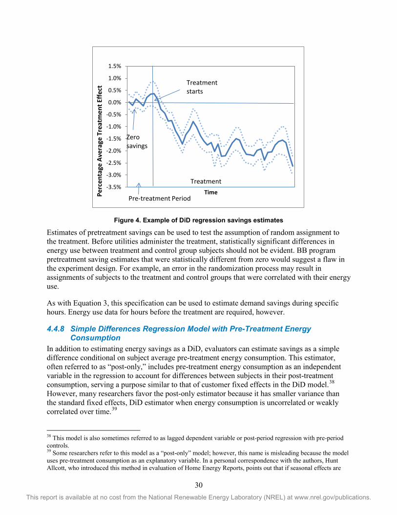
30 This report is available at no cost from the National Renewable Energy Laboratory (NREL) at www.nrel.gov/publications.
Figure 4. Example of DiD regression savings estimates
Estimates of pretreatment savings can be used to test the assumption of random assignment to the treatment. Before utilities administer the treatment, statistically significant differences in energy use between treatment and control group subjects should not be evident. BB program pretreatment saving estimates that were statistically different from zero would suggest a flaw in the experiment design. For example, an error in the randomization process may result in assignments of subjects to the treatment and control groups that were correlated with their energy use.
As with Equation 3, this specification can be used to estimate demand savings during specific hours. Energy use data for hours before the treatment are required, however.
4.4.8 Simple Differences Regression Model with Pre-Treatment Energy Consumption
In addition to estimating energy savings as a DiD, evaluators can estimate savings as a simple difference conditional on subject average pre-treatment energy consumption. This estimator, often referred to as “post-only,” includes pre-treatment energy consumption as an independent variable in the regression to account for differences between subjects in their post-treatment consumption, serving a purpose similar to that of customer fixed effects in the DiD model.38 However, many researchers favor the post-only estimator because it has smaller variance than the standard fixed effects, DiD estimator when energy consumption is uncorrelated or weakly correlated over time.39
38 This model is also sometimes referred to as lagged dependent variable or post-period regression with pre-period controls. 39 Some researchers refer to this model as a “post-only” model; however, this name is misleading because the model uses pre-treatment consumption as an explanatory variable. In a personal correspondence with the authors, Hunt Allcott, who introduced this method in evaluation of Home Energy Reports, points out that if seasonal effects are
-3.5%
-3.0%
-2.5%
-2.0%
-1.5%
-1.0%
-0.5%
0.0%
0.5%
1.0%
1.5%
Perc
enta
ge A
vera
ge T
reat
men
t Effe
ct
Time
Treatment
Pre-treatment Period
Treatment starts
Zero savings

31 This report is available at no cost from the National Renewable Energy Laboratory (NREL) at www.nrel.gov/publications.
Consider the following regression specification:
Equation 7 yit = τt + β1*Trit + 𝜌𝜌𝑦𝑦𝚤𝚤
𝑝𝑝𝑝𝑝𝑝𝑝������ + εit
Where:
τt = The time-period fixed effect (an unobservable that affects consumption of all subjects during time period t). The time period effect can be estimated by including a separate dummy variable for each time period t, where t = -T, -T+1, …, -1, 0, 1, 2, ..., T.
β1 = Coefficient for the average treatment effect of the program. The energy savings per subject per period equals -β1.
Trit = An indicator variable for whether subject i received the treatment in period t. The variable equals 1 for subjects who receive the treatment in period t and equals 0 otherwise.
ρ = Coefficient indicating the effect of average pre-treatment consumption on consumption during the treatment period.
𝑦𝑦𝚤𝚤𝑝𝑝𝑝𝑝𝑝𝑝������ = Average consumption during the pre-treatment period for subject i.
εit = The model error term, representing random influences on the energy use of customer i in period t.
With random assignment of subjects to treatment and control groups, the OLS estimation of Equation 6 is expected to produce an unbiased estimate of the average savings per subject per period.
Evaluators can estimate slightly different versions of this model:
• Savings for each treatment period. Evaluators can include a treatment indicator variable for each period instead of a treatment indicator variable for the entire treatment period. This specification will produce an estimate of average savings per subject for each treatment period.
• Additional pre-treatment consumption control variables. Instead of one pre-treatment consumption variable, evaluators can include multiple pre-treatment consumption variables, such as variables for different seasons or months of a year, days of week, or hours of the day.
• Additional control variables. Evaluators can add other variables such as weather to the model. The addition of such variables might help to improve the precision of the savings estimates.
being estimated, this model “has slightly smaller standard errors and can be better at addressing naturally occurring randomization imbalances that may result in the baseline pretreatment energy usage differing between the control and treatment group.”

32 This report is available at no cost from the National Renewable Energy Laboratory (NREL) at www.nrel.gov/publications.
4.4.9 Randomized Encouragement Design Some field experiments involve an RED in which subjects are only encouraged to accept a BB measure, in contrast to RCTs in which a program administers a BB intervention. This section outlines the types of regression models that are appropriate for REDs, how to interpret the coefficients, and how to estimate savings from RED programs.
Evaluators can apply the model specifications previously described for RCTs to REDs. The model coefficients and savings are interpreted differently, however, and an additional step is required to estimate average savings for subjects who accept the behavioral intervention. Treatment in an RED is defined as receiving encouragement to adopt the BB intervention, rather than actually receiving the intervention as with RCTs.
Consider a field experiment with an RED that has energy consumption data for treatment and control group subjects available for the pretreatment and treatment periods. Equations 1 through 4 can be used to estimate the treatment effect, or the average energy consumption effect on those receiving encouragement. The estimate captures savings from compliers only, because never takers never accept the intervention, and always takers would accept the intervention with or without encouragement.
To recover the LATE, the savings from subjects who accept the treatment because of the encouragement, scale the estimate of β2 by the inverse of the difference between the percentage of subjects in the treatment group who accept the intervention and the percentage of subjects in the control group who accept the intervention (which is zero if control group subjects are prohibited from accepting the intervention). Estimate this as:
Equation 8 β2 /(πT – πC)
Where:
πT = The percentage of treatment group subjects who accept the intervention.
πC = The percentage of control group subjects who accept the intervention.
A related approach for obtaining an estimate of savings for the BB intervention in a RED study is instrumental variables, two-stage least squares (IV-2SLS). This approach uses the random assignment of subjects to the treatment as an instrumental variable for the decision by encouraged customers to participate in the program. The instrumental variable provides the exogenous variation necessary to identify the effect of endogenous participation on energy consumption. Participation is endogenous because the encouraged customers’ decisions to participate is not random and depends on unobserved characteristics that may be correlated with energy consumption. For encouragement to be a valid instrument, it must be that encouragement affects only energy consumption through its impact on BB program participation.
In the first stage, the evaluator regresses a binary program participation decision variable on an indicator for whether the customer was randomly assigned to receive encouragement and other exogenous independent variables from the second-stage energy consumption equation. The evaluator then uses the regression to predict the likelihood of participation for each subject and time period. In the second stage, the evaluator estimates the energy consumption equation,
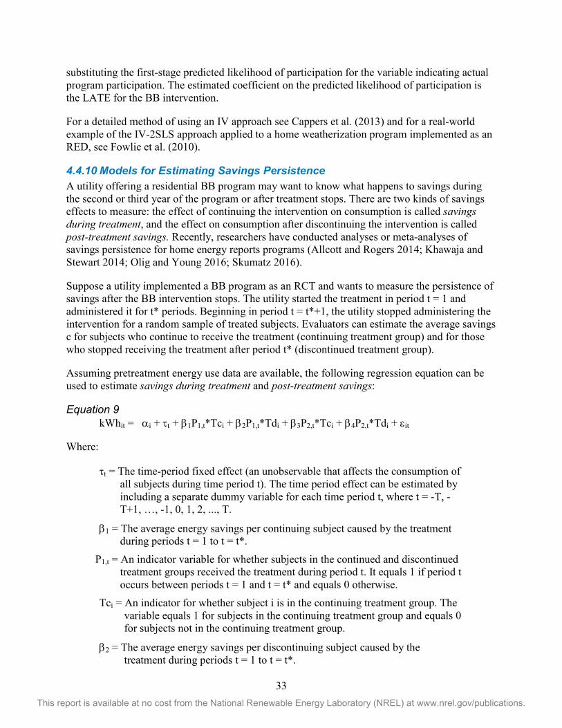
33 This report is available at no cost from the National Renewable Energy Laboratory (NREL) at www.nrel.gov/publications.
substituting the first-stage predicted likelihood of participation for the variable indicating actual program participation. The estimated coefficient on the predicted likelihood of participation is the LATE for the BB intervention.
For a detailed method of using an IV approach see Cappers et al. (2013) and for a real-world example of the IV-2SLS approach applied to a home weatherization program implemented as an RED, see Fowlie et al. (2010).
4.4.10 Models for Estimating Savings Persistence A utility offering a residential BB program may want to know what happens to savings during the second or third year of the program or after treatment stops. There are two kinds of savings effects to measure: the effect of continuing the intervention on consumption is called savings during treatment, and the effect on consumption after discontinuing the intervention is called post-treatment savings. Recently, researchers have conducted analyses or meta-analyses of savings persistence for home energy reports programs (Allcott and Rogers 2014; Khawaja and Stewart 2014; Olig and Young 2016; Skumatz 2016).
Suppose a utility implemented a BB program as an RCT and wants to measure the persistence of savings after the BB intervention stops. The utility started the treatment in period t = 1 and administered it for t* periods. Beginning in period t = t*+1, the utility stopped administering the intervention for a random sample of treated subjects. Evaluators can estimate the average savings c for subjects who continue to receive the treatment (continuing treatment group) and for those who stopped receiving the treatment after period t* (discontinued treatment group).
Assuming pretreatment energy use data are available, the following regression equation can be used to estimate savings during treatment and post-treatment savings:
Equation 9 kWhit = αi + τt + β1P1,t*Tci + β2P1,t*Tdi + β3P2,t*Tci + β4P2,t*Tdi + εit
Where:
τt = The time-period fixed effect (an unobservable that affects the consumption of all subjects during time period t). The time period effect can be estimated by including a separate dummy variable for each time period t, where t = -T, -T+1, …, -1, 0, 1, 2, ..., T.
β1 = The average energy savings per continuing subject caused by the treatment during periods t = 1 to t = t*.
P1,t = An indicator variable for whether subjects in the continued and discontinued treatment groups received the treatment during period t. It equals 1 if period t occurs between periods t = 1 and t = t* and equals 0 otherwise.
Tci = An indicator for whether subject i is in the continuing treatment group. The variable equals 1 for subjects in the continuing treatment group and equals 0 for subjects not in the continuing treatment group.
β2 = The average energy savings per discontinuing subject caused by the treatment during periods t = 1 to t = t*.

34 This report is available at no cost from the National Renewable Energy Laboratory (NREL) at www.nrel.gov/publications.
Tdi = An indicator for whether subject i is in the discontinuing treatment group. The variable equals 1 for subjects in the discontinuing treatment group and equals 0 for subjects not in the discontinuing treatment group.
β3 = The average energy savings from the treatment for subjects in the continuing treatment group when t>t*.
P2,t = An indicator variable for whether continuing treatment group subjects received the treatment and discontinued treatment group subjects did not receive the treatment during period t. It equals 1 if period t occurs after t = t* and equals 0 otherwise.
β4 = The average energy savings for subjects in the discontinued treatment group when t>t*.
The OLS estimation of Equation 9 yields unbiased estimates of savings during treatment (β3) and post-treatment savings (β4) because original treatment group subjects were assigned randomly to the continuing and discontinued treatment groups. Evaluators can expect that β4 ≥ β3, that is, the average savings of the continuing treatment group will be greater than that of the discontinued treatment group. To estimate savings decay after treatment stops, evaluators can take the difference between savings during treatment (β2) and post-treatment savings (β4) for subjects in the discontinued treatment group.
Evaluators can test the identifying assumption of random assignment to the discontinued treatment group by comparing the savings of continuing and discontinuing treatment group subject between period t = 1 and t*. If assignment was random, their savings during this period are expected to be equal.
4.4.11 Standard Errors Panel data have multiple energy use observations for each subject; thus, the energy use data are very likely to exhibit within-subject correlations. Many factors affecting energy use persist over time, and the strength of within-subject correlations usually increases with the frequency of the data. When standard errors for panel regression model coefficients are calculated, these correlations must be accounted for. Failing to do so will lead to savings estimates with standard errors that are biased downward.
This protocol strongly recommends that evaluators estimate robust standard errors clustered on subjects (the randomized unit in field trials) to account for within-subject correlation. Most statistical software programs, including STATA, SAS, and R, have regression packages that output regression-clustered standard errors.
Clustered standard errors account for having less information about energy use in a panel with N subjects and T observations per subject than in a dataset with N*T independent observations. Because clustered standard errors account for these within-subject energy-use correlations, they are typically larger than OLS standard errors. When there is within-subject correlation, OLS

35 This report is available at no cost from the National Renewable Energy Laboratory (NREL) at www.nrel.gov/publications.
standard errors are biased downward and overstate the statistical significance of the estimated regression coefficients.40
4.4.12 Opt-Out Subjects and Account Closures Many BB programs allow subjects to opt out and stop receiving the treatment. This section addresses how evaluators should treat opt-out subjects in the analysis, as well as subjects whose billing accounts close during the analysis period.
As a general rule, evaluators should include all subjects initially assigned to the treatment and control groups in the savings analysis.41 For example, evaluators should keep opt-out subjects in the analysis sample. Opt-out subjects may have different energy use characteristics than subjects who remain in the program, and dropping them from the analysis would result in nonequivalent treatment and control groups. To ensure the internal validity of the savings, opt-out subjects should be kept in the analysis sample.
Sometimes treatment or control group subjects close their billing accounts after the program starts. Account closures are usually unrelated to the BB program or savings; most are due to households changing residences. Subjects in the treatment group should experience account closures for the same reasons and at the same rates as subjects in the control group; evaluators can thus safely drop treatment and control group subjects who close their accounts from the analysis sample.
However, if savings are correlated with the probability of an account closure, it may be best to keep subjects with account closures in the analysis sample. For example, if young households, which are the most mobile and likely to close their accounts, are also most responsive to BB programs, dropping these households from the analysis would bias the savings estimates downward,42 and evaluators should keep these households in the analysis.
If evaluators drop customers who close their accounts during the treatment from the regression estimation, they should still count the savings from these subjects for periods during the treatment before customers closed their accounts. To illustrate, when estimating savings for a 1-year BB program, evaluators can estimate the savings from subjects who closed their accounts and from those who did not as the weighted sum of the conditional average program treatment effects in each month:
Equation 10 Savings = ∑m = 1
12 -βm * Daysm* Nm
Where: m = Indexes the months of the year
40 Bertrand et al. (2004) show when DiD studies ignore serially correlated errors, the probability of finding significant effects when there are none (Type I error) increases significantly. 41 This protocol urges evaluators not to arbitrarily drop outlier energy use observations from the analysis unless energy use was measured incorrectly. If an outlier is dropped from the analysis, the reasons for dropping the outlier and the effects of dropping it from the analysis on the savings estimates should be clearly documented. Evaluators should test the sensitivity of the results to dropping observations. 42 See State and Local Efficiency Action Network (2012), p. 30.

36 This report is available at no cost from the National Renewable Energy Laboratory (NREL) at www.nrel.gov/publications.
-βm = The conditional average daily savings in month m (obtained from a regression equation that estimates the program treatment effect on energy use in each month)
Daysm = The number of days in month m
Nm = The number of subjects with active accounts receiving the treatment in month m or in a previous month.
This approach assumes that savings in a given month for subjects who close their accounts are equal to savings of subjects whose accounts remain open.
4.5 Energy Efficiency Program Uplift and Double Counting of Savings Many BB programs increase participation in other utility energy efficiency programs; this additional participation is known as efficiency program uplift. For example, many utilities encourage their energy report program recipients to participate in their other energy efficiency programs that provide cash rebates in exchange for adopting efficiency measures such as efficient furnaces, air conditioners, wall insulation, windows, and compact fluorescent lamps.
Quantifying the effects of BB programs on efficiency program participation is important for two reasons:
• Uplift can be an important effect of BB programs and a potential additional source of energy savings.
• Savings from efficiency program uplift could be double-counted if unaccounted for. That is, when a household participates in an efficiency program because of a BB program intervention, the utility may count the program savings twice: once in the regression-based estimate of BB program savings and again in the estimate of savings for the rebate program. To avoid double-counting savings, evaluators must estimate savings from program uplift and subtract these savings from the efficiency program portfolio savings.43
Estimating savings from BB program uplift with randomized experiments recommended in this protocol is conceptually straightforward. To illustrate, suppose that a utility markets energy efficiency Measure A to treatment and control group subjects identically through a separate rebate program. Subjects in the treatment group also receive behavioral messaging encouraging them to adopt efficiency measures, including Measure A. Because customers were randomly assigned to the treatment and control groups, the groups are expected to be equivalent except for the treated customers who received the behavior treatment. Therefore, evaluators can attribute any difference in the uptake of Measure A between the groups to the BB program.
43 This protocol does not take a position on which program gets credit for the uplift. When a BB intervention causes participation in an energy efficiency program, we know that the program participation would not have occurred without the intervention. However, the amount of uplift caused by the BB intervention may depend on the dollar incentives provided by the efficiency program. For example, the BB program may produce greater lift in participation for a program incentive of $200 than $100. To determine the relationship between uplift and the incentive amount, it would be necessary to randomize the incentive amount and to study participation as a function of incentives and who receives the BB intervention.

37 This report is available at no cost from the National Renewable Energy Laboratory (NREL) at www.nrel.gov/publications.
Figure 5 illustrates this logic for calculating behavior program savings from efficiency program uplift. Behavior program savings from adoption of Measure A is the difference between the treatment group and the control group in savings from Measure A.
Figure 5. Calculation of double-counted savings
To estimate BB program savings from efficiency program uplift, evaluators should take the following steps:
1. Match the BB program treatment and control group subjects to the utility energy efficiency program tracking data.
2. Calculate the uplift savings per treatment group subject as the difference between treatment and control groups in average efficiency program savings per subject, where the savings are obtained from the utility tracking database of installed measures. (The averages should be calculated over all treatment group subjects and all control group subjects, not just those who participated in efficiency programs.)
3. Multiply the uplift savings per treatment group customer by the number of subjects who were in the treatment group to obtain the total uplift savings.
Evaluators can estimate BB program savings from efficiency program uplift for efficiency measures that the utility tracks at the customer level. Most measures for which utilities offer rebates—such as high-efficiency furnaces, windows, insulation, and air conditioners—fit this description.
Evaluators should be mindful of specific reporting conventions for efficiency program measures in utility tracking databases. For example, many jurisdictions require utilities to report weather-normalized and annualized measure savings, which do not reflect when measures were installed during the year or the actual weather conditions that affected savings. In contrast, the regression-based estimate of energy savings will reflect installation dates of measures and actual weather.
Control Group Treatment Group
Ener
gy sa
ving
s fro
m u
tility
reba
te p
rogr
ams
(kW
h)
Caused by behaviorprogram
Naturally occuringUplift savings = savings from rebated measures caused by behavior program

38 This report is available at no cost from the National Renewable Energy Laboratory (NREL) at www.nrel.gov/publications.
Evaluators should therefore adjust the annualized deemed savings in the program reporting database to account for when measures were installed during the year.
In addition, for BB programs running longer than one year, evaluators should account for the savings impacts of program uplift in previous years. Measures with a multiyear life installed in a previous program year will continue to save energy in subsequent years. Depending on the utility’s conventions for reporting savings, it may be necessary to subtract savings from uplift in previous years from BB program savings estimate.
Estimating savings from program uplift for measures that the utility does not track at the customer level is more challenging. The most important such measures are high-efficiency lights such as compact fluorescent lamps and light-emitting diodes that are rebated through utility upstream programs. Most utilities provide incentives directly to retailers for purchasing these measures, and the retailers then pass on these price savings to utility customers in the form of retail discounts. Data on the purchases of rebated measures by treatment and control group subjects must be collected to estimate BB savings in upstream efficiency programs. Evaluators can use household surveys for this purpose.44 However, because the difference in the number of purchased bulbs between treatment and control group subjects may be small, it may be necessary to survey a very large number of subjects to detect the BB program effect. Also, evaluators should adjust the lighting purchases impact estimates for in-service rates and the percentage of high efficiency lamps sold in the utility service area that received rebates. Evaluators should also be aware that some energy savings from purchasing compact fluorescent lamps or light-emitting diodes may be offset by reductions in the hours of use of those bulbs by treated customers.
44 For an example of the approach required to estimate BB program savings from adoption of compact fluorescent lamps, see PG&E (2013).
39 This report is available at no cost from the National Renewable Energy Laboratory (NREL) at www.nrel.gov/publications.
5 Reporting BB program evaluators should carefully document the research design, data collection and processing steps, analysis methods, and plan for calculating savings estimates. Specifically, evaluators should describe:
• The program implementation and the hypothesized effects of the behavioral intervention
• The experimental design, including the procedures for randomly assigning subjects to the treatment or control group
• The sample design and sampling process
• Processes for data collection and preparation for analysis, including all data cleaning steps
• Analysis methods, including the application of statistical or econometric models and key assumptions used to identify savings, including tests of those key identification assumptions
• Results of savings estimate, including point estimates of savings and standard errors and full results of regressions used to estimate savings.
A good rule-of-thumb is that evaluators should report enough detail such that a different evaluator could replicate the study with the same data. Every detail does not have to be provided in the body of the report; many of the data collection and savings estimation details can be provided in a technical appendix.

40 This report is available at no cost from the National Renewable Energy Laboratory (NREL) at www.nrel.gov/publications.
6 Looking Forward Evaluators and program administrators should employ randomized experiments for evaluating BB programs whenever possible. However, some BB programs may be difficult or costly to evaluate using randomized experiments. In these cases, evaluators must employ quasi-experiments that rely on random but uncontrolled variation in who participates.
An important question concerns the accuracy of quasi-experimental methods such as propensity-score matching, regression discontinuity, and DiD estimation for evaluating BB programs. Evaluators of BB programs have employed and will continue to employ these methods. Although this protocol has cited several studies comparing the accuracy of randomized experiments and quasi-experiments, more research will be needed to draw firm conclusions about the accuracy of quasi-experiments.
Depending on the outcome of this research and acceptance by regulators and program administrators of savings estimates from quasi-experiments, evaluators could give consideration to updating this protocol to include quasi-experimental methods.

41 This report is available at no cost from the National Renewable Energy Laboratory (NREL) at www.nrel.gov/publications.
7 References Allcott, H. (2015). “Site Selection Bias in Program Evaluation.” The Quarterly Journal of Economics 130 (3), pp. 1117-1165. Allcott, H. (2011). “Social Norms and Energy Conservation.” Journal of Public Economics, 95(2), pp. 1082-1095.
Allcott, H.; Rodgers, T. (2014). “The Short-Run and Long-Run Effects of Behavioral Interventions: Experimental Evidence from Energy Conservation.” American Economic Review 104 (10), pp. 3003-3037.
Baylis, P.; Cappers, P.; Jin, L.; Spurlock, A.; Todd, A. (2016). “Go for the Silver? Evidence from field studies quantifying the difference in evaluation results between “gold standard” randomized controlled trial methods versus quasi-experimental methods.” ACEEE Summer Study on Energy Efficiency in Buildings 2016.
Bertrand, M.; Duflo, E.; Mullainathan, S. (2004). “How Much Should We Trust Difference-in-Differences Estimates?” Quarterly Journal of Economics 119 (1), 249–275.
Brandon, A.; Ferraro, P. J.; List, J. A.; Metcalfe, R. D.; Price, M. K.; Rundhammer, F. (2017). Do the Effects of Social Nudges Persist? Theory and Evidence from 38 Natural Field Experiments. National Bureau of Economic Research working paper 23277. Available at: http://www.nber.org/papers/w23277
Bruhn, M., McKenzie D. (2009). “In Pursuit of Balance: Randomization in Practice in Development Field Experiments.” American Economic Journal: Applied Economics 1(4): 200-232.
Burlig, F., Preonas, L., Woerman, M. (2017). Panel Data and Experimental Design. Energy Institute at Haas working paper. Available at: https://ei.haas.berkeley.edu/research/papers/WP277.pdf
Cappers, P.; Todd, A.; Perry, M.; Neenan, B.; Boisvert, R. (2013). Quantifying the Impacts of Time-based Rates, Enabling Technology, and Other Treatments in Consumer Behavior Studies: Protocols and Guidelines. Lawrence Berkeley National Laboratory, Berkeley, CA and the Electric Power Research Institute, Palo Alto, CA. LBNL-6301E. Available at: https://emp.lbl.gov/sites/default/files/lbnl-6301e.pdf
Costa, D.L.; Kahn, M.E. (2010). Energy Conservation “Nudges” and Environmentalist Ideology: Evidence from a Randomized Residential Electricity Field Experiment. NBER Working Paper 15939. Available at: http://www.nber.org/papers/w15939
Consortium for Energy Efficiency Database (2013). Available at: http://library.cee1.org/content/2013-behavior-program-summary-public-version
Davis, M. (2011). Behavior and Energy Savings: Evidence from a Series of Experimental Interventions. Environmental Defense Fund Report.

42 This report is available at no cost from the National Renewable Energy Laboratory (NREL) at www.nrel.gov/publications.
EPRI (2010). Guidelines for Designing Effective Energy Information Feedback Pilots: Research Protocols. Electric Power Research Institute: Palo Alto, CA. 1020855.
Fowlie, M. (2010). U.S. Department of Energy Smart Grid Investment Grant Technical Advisory Group Guidance Document #7, Topic: Design and Implementation of Program Evaluations that Utilize Randomized Experimental Approaches. November 8, 2010.
Frison, L.; Pocock, S. J. (1992). “Repeated measures in clinical trials: Analysis using mean summary statistics and its implications for design.” Statistics in Medicine 11.13 (1992): pp. 1685-704.
Greene, W. (2011). Econometric Analysis. New Jersey: Prentice Hall.
Harding, M.; Hsiaw, A. (2012). Goal Setting and Energy Efficiency. Stanford University working paper.
Ignelzi, P.; Peters, J.; Dethman, L.; Randazzo, K.; Lutzenhiser, L. (2013). Paving the Way for a Richer Mix of Residential Behavior Programs. Prepared for Enernoc Utility Solutions. CALMAC Study SCE0334.01.
Khawaja, M.S., Stewart, J. (2015). Long-Run Savings and Cost Effectiveness of Home Energy Report Programs. Cadmus Research Report. Available at: http://www.cadmusgroup.com/wp-content/uploads/2014/11/Cadmus_Home_Energy_Reports_Winter2014.pdf
List, J.A. (2011). “Why Economists Should Conduct Field Experiments and 14 Tips for Pulling One Off.” Journal of Economic Perspectives (25), pp. 3–16.
List, J.A., Sadoff, S.; Wagner, M. (2010). So You Want to Run an Experiment, Now What? Some Simple Rules of Thumb for Optimal Experimental Design. National Bureau of Economic Research Paper 15701.
Mazur-Strommen, S.; Farley, K. (2013). ACEEE Field Guide to Utility-Run Behavior Programs. American Council for an Energy Efficient Economy, Report Number B132.
Minnesota Department of Commerce, Division of Energy Resources (2015). Energy Efficiency Behavioral Programs: Literature Review, Benchmarking Analysis, and Evaluation Guidelines. Prepared by Illume Advising with subcontractors Indica Consulting and Dr. Edward Vine. Available at: http://mn.gov/commerce-stat/pdfs/card-report-energy-efficiency-behavorial-prog.pdf
National Renewable Energy Laboratory. (2017). Strategic Energy Management Protocol: The Uniform Methods Project. Prepared by James Stewart. Available at: https://www.nrel.gov/docs/fy17osti/68316.pdf
Olig, C.; Young, E. 2016. ComEd Home Energy Report Program Decay Rate and Persistence Study – Year Two. Navigant.
PG&E (2013). 2012 Load Impact Evaluation for Pacific Gas and Electric Company’s SmartAC Program. Prepared by Freeman, Sullivan & Co.

43 This report is available at no cost from the National Renewable Energy Laboratory (NREL) at www.nrel.gov/publications.
PSE (2012). Home Energy Reports Program: Three Year Impact Behavioral and Process Evaluation. Puget Sound Energy. Prepared by DNV GL.
Rosenberg, M.; Kennedy Agnew, G.; Gaffney, K. (2013). Causality, Sustainability, and Scalability – What We Still Do and Do Not Know about the Impacts of Comparative Feedback Programs. Paper prepared for 2013 International Energy Program Evaluation Conference, Chicago.
SEE Action (2012). Evaluation, Measurement, and Verification (EM&V) of Residential Behavior-Based Energy Efficiency Programs: Issues and Recommendations. State and Local Energy Efficiency Action Network. Prepared by A. Todd, E. Stuart, S. Schiller, and C. Goldman, Lawrence Berkeley National Laboratory. http://behavioranalytics.lbl.gov. Available at: https://www4.eere.energy.gov/seeaction/system/files/documents/emv_behaviorbased_eeprograms.pdf
Seelig, M.J. (2013) “Business Energy Reports” presentation at BECC 2013. Available at: http://beccconference.org/wp-content/uploads/2013/12/BECC_PGE_BER_11-19-13_seelig-.pdf
Shadish, W.R., Cook, T.D.; Campbell, D.T. (2002). Experimental and Quasi-experimental Designs for Generalized Causal Inference. Belmont, CA: Wadsworth Cengage Learning.
Skumatz, L. (2016). Persistence of Behavioral Programs: New Information and Implications for Program Optimization. The Electricity Journal 29 (5): pp. 27-32.
SMUD (2013). SmartPricing Options Interim Evaluation. Prepared for the U.S. Department of Energy and Lawrence Berkeley National Laboratory by Sacramento Municipal Utility District and Freeman, Sullivan, & Co.
SMUD (2011). Sacramento Municipal Utility District Home Energy Report Program Impact and Persistence Evaluation Report, Years 2008-2011. Prepared by May Wu, Integral Analytics.
Stewart, J. (2013a). Peak-Coincident Demand Savings from Behavior-Based Programs: Evidence from PPL Electric's Behavior and Education Program. UC Berkeley: Behavior, Energy and Climate Change Conference. Available at: http://escholarship.org/uc/item/3cc9b30t.
Stewart, J. (2013b). “Energy Savings from Business Energy Feedback.” Presentation at BECC 2013. Available at: http://beccconference.org/wp-content/uploads/2015/10/presentation_stewart.pdf.
Todd, A. (2014). Insights from Smart Meters: The Potential for Peak-Hour Savings from Behavior-Based Programs. Lawrence Berkeley National Laboratory. LBNL Paper LBNL-6598E. Available at: http://escholarship.org/uc/item/2nv5q42n