chapter 15 irrigation - usda · chapter 15 irrigation introduction irrigation is the application of...
TRANSCRIPT

Chapter 15 Irrigation
- Contents
Introduction ........................................................................ 15-l Advantagesofirrigation .............................................................. 15-l Requirements for SUCCe88fI.d irrigation .................................................. 15-2 Factor8 in planning ................................................................... 15-3
Shl8 ............................................................................. 15-3 Topography ........................................................................ 15-3 Water8upply ...................................................................... 15-3 Erosion control and drainage.. ....................................................... 15-6 Farm andranch ente~ri~s.......................- .................................. 15-6 Economics*............................-...- ........................................ 15-6
Basic design criteria. .................................................................. 15-7 Irrigation method8 ................................................................... 15-B
Levelborders.. .................................................................... 15-B Gradedborders .................................................................... 15-B FurrOW .......................................................................... 15-B
Graded f~ows...................~.........................-...................- . .15-B Contour furrows ................................................................... 15-B
Corrugation8 ...................................................................... 15-Q Contour Ditch ..................................................................... 15-9 Sprinkle .......................................................................... 15-9 Subirrigation ...................................................................... 15-9 Trickle ........................................................................... 15-Q
Wa~rconveyance.....................................-.........................- .... 15-12 Capacity ......................................................................... 15-12 Openditches ........................................................................ 15-12 st~ct~eB...................* ..................................................... 15-12 Drop8 ............................................................................ 15-12 Pipe~neB............................-.....................- ....................... 15-13 Measuring de~ce8................*-...*.........**-....................- ........... 15-13
Landleveling.. ..................................................................... 15-14 Water di8posaI system....................................................- ........... 15-14 Equipment.......“........-...........~.......-.- ................................... 15-15
Checkdams.. ..................................................................... 1515 Siphon tubes ...................................................................... 15-15 Gatedpipe ........................................................................ 15-15
Methods of measuring or estimating soil moisture ......................................... 15-16 Irrigation water management .......................................................... 1517
Introduction.. ..................................................................... 15-17 Ra8ic soil-moisture-plant relationships ................................................. 15-17
Available water capacity .......................................................... 15-17 Cropr~tzonedept~.........-...................*........~...............*....- . 15-18 Plant moi8ture requirements ...................................................... 15-18 Consumptive use ra~8...............................-........................*.- . 15-18
~valuationpr~ed~e ................................................................ 15-19 Need for irrigation and amount to apply ............................................. 15-19 Amount applied ................................................................. 15-19 Field application efficiency ........................................................ 15-22 Uniformity of application ......................................................... 15-23 Estimating rate8 offlow .......................................................... 15-29 Soilerosion.. ................................................................... 15-29
15-i
Special problems. .................................................................. Irrigation at high moisture levels. ................................................. Lateral spread of water .......................................................... Leaching ...................................................................... Overall water resource use .......................................................
Moisture accounting method for scheduling irrigation .................................... Use .............................................................................. B~icp~nciples............................................* ....................... Cond~ionsforuse.......~......~..~......................~..* ...................... Equipment required ................................................................ Installation and reading of the rain gage. ........................... , ................. Use of the moisture balance sheet for scheduling irrigation. .............................
Beginning moisture balance. ...................................................... Determining end-of-day moisture balance. ............................................ Adjustment factors .............................................................. Irrigationprocedure .............................................................
Direct gas pressure method for scheduling imigation ...................................... Sample problem................................................*..........* ........ Moisture percentage at field capacity .................................................. Bulkde~~yme~~ement*.......* .................................................. Moisture percentage at wilting point .................................................. Centimeters (inches) of available moisture .............................................. Net moisture requirement at each moisture level ........................................ Determining adjustment percentages .. : ............................................... Dry weight moisture percentages at each moisture level ................................ Gage readings for each dry weight moisture percentage ................................. Checking and recording soil moisture .................................................. Use of the Soil Characteristics Sheet ..................................................
E~ibi~..............**................*....................*.........*.........* ..
15-ii
Puge
15-30 15-30 15-30 15-31 16-31 X-32 15-32 15-32 15-32 15-32 15-32 15-33 15-33 15-33 15-42 15-42 1543 1543 1545 15-45 15-46 15-46 15-46 1546 15-47 15-47 15-47 1547 15-49
a
0
a

FQures
16-l Some elementa considered in irrigation planning. .............................. 154 15-2 Basic component of a trickle irrigation system. ................................ 15-10 15-3 Typical two-Btation, split-flow layout for a trickle irrigation system with
blocks I and III, or II and N operating simultaneowly ......................... 16-11 154 and 4A Sample advance and receaion curves ........................................ 15-23 15-5and5A Sampleintakecurve.. ..................................................... 15-28 15-6 Samplingoftexturallayers,. ............................................... 1645
Tables
16-l General range of available moisture-holding capacities and average design vaIuea for normal soil condition . . . . . , . . . . . . . , . , . . . . . . . . . . . . . . . . . e . . . . . . . b . . . . . . . . , . . 15-18
15-2 Computatiou of runoff volume . . . . . . m . . . . . . . . . . . . . . . . . . . . . . . . . . . a . . . . . . , . . . . 16-28 16-3 Soil factors for estimating average intake rata from finaI intie rate . . . . . . . . . . . . . 15-28 15-4 and 4A Moisture balance for scheduling irrigation . . . a . . . . . . . . . . . . . . . . . . . . . . . . . . . . , . . . m 1534 15-5 Sample-Estimated values of daily evapotian@ration for observed sunshine and
crop stage of growth. . . . ..*.........*......**.......*......*..*.*....*..... 1542 15-8 Soil Characteristic Sheet for irrigation water management . , . . . . . . . . . . . . . . . . . . . 1544 15-7 Field moisture check sheet for determining when to irrigate and
how much water to apply . . . . . . . , . . . . . . . , , . . . . ..,.*.......*....*........,.* 1648
Exhibits
15-l 15-2 15-3 15-4 16-5 15-8 15-7 and 7A
Irrigation ditch sections with required lateral beti ............................. 16-60 Beliefclmsforsurface-irrigatedland. ................... . .................. 16-51 Discharge of aluminum siphon tubes at various heads .......................... 16-52 Multiple outlet factor for gated pipe ......................................... 15-62 Feel and appearance method of estimating available moisture ................... 1553 Carbide moisture tater conversion chart ..................................... 15-55 Equivalent moisture table for relating available moiBtu.re level to net centimeter6 (inches) of water to apply ..................................... l&St3
15.iii
Chapter 15 Irrigation
Introduction
Irrigation is the application of water to the land to provide adequate moisture for crop production. This practice includes the development of the water supply, the conveyance system, the method of ap- plication, and the waste water disposal system, along with the necessary management to achieve the intended purpose.
Irrigation is necessary because rainfall otin does not occur at the appropriate time or is inadequate for crop needs. Rainfall distribution is seldom ideal during the growing season. In the more arid parts of the United States, rainfall during the growing season is far short of most crop needs. Even in areas of high seasonal rainfall, crops often suffer from a lack of moisture for short perk& during some part of the growing season,
A drought period can be defined as any number of consecutive days in which the available moisture in the soil has been so reduced by plant use and sur- face evaporation that plant growth’ and quality are adversely affected. The i-1 between a max- imum supply of available moisture and the begin- ning of a drought period varies widely. This inter- val depends on the ability of the soil to store moisture, the rooting habits of the crop, the in- cidence of rainfall, and the evapotranspiration rate. See Chapters 1 and 3, Section 16, SCS National Engineering Handbook,
Advantages of Irrigation
Many benefits are obtained from the proper use of irrigation. Where lack of moisture would limit crop production, irrigation can be expected to increase crop yields. And, by careful control of the amount of moisture in the soil, higher quality crops that bring higher market prices can be produced each year. For example, irrigation can be used to counteract high or low temperatures; to eliminate short droughts that reduce quality; or, by being withheld, to allow a curing-out period prior to harvest.
For certain crops, particularly fruits and vegetables, the difference between profit and loss often depends on the time the crop reaches the market. Roper irrigation aids prompt germination and continuous plant growth, making it possible to regulate planting dates and time of maturity more closely.
Fertilizers do not increase plant growth unless moisture is available. With irrigation, fertilizers can be made available for plant use almost im- mediately and more of the fertilizer applied may be used effectively. Applying soluble fertilizers through irrigation water is a common practice. With sprinkle irrigation, this practice offers a sav- ing in labor, requires a minimum of fertilizing equipment, and the depth of penetration can be closely controlled.
High-value cash crops, such as strawberries, cranberries, tomatoes, and citrus, can be provided some protection from frost and freeze damage through water applications just before and during periods of freezing temperatures.
Applying irrigation water immediately following transplanting greatly increases plant survival, thereby reducing costs of replacing plants. The water settles the soil into close contact with the r& system. Sometimes an application is made just before transplanting if soil moisture is not up to field capacity.
Efficient irrigation promotes better use of the land in accordance with its capabilities and stabilizes yields of adapted crops. Irrigation also makes possible the seeding and prompt germination of soil improvement crops at the propr time during the growing season and helps te establish vegetitive cover on eroded areas.
15-l

Requirements for Successful Irrigation
For additional guidance on application of fer- tili&rs, soil amendments, and frost control, see SCS National Engineering Handbook, Section 15.
Irrigation dms not necessarily ensure high crop yields and lsrge profits. It should be used only on those soils that, if properly treated and managed, are capable of producing sustained high yields of ir- rigated crops. These soils are indicated in irrigation guides.
The water supply must be large enough to meet crop needs on the acreage to be irrigated and must be of suitable quality. The water must also be both economically accessible and legally available to the irrigator.
The irrigation system must be designed to divert water from the supply source, deliver it to the ir- rigated area, and apply it to the crop in an amount and rate that will meet consumptive use require- ments of the crop without causing erosion or other damage to the land. The designed system should be practical, durable, and efficient.
The addition of irrigation to a farming operation usually increases labor and capital requirements. Very oRen labor is required for irrigation at a time when other crops must be planted, cultivated, or h-e&d. Additional capital is required both for the initial installation of the irrigation system and the operation and maintenance of the system, at least through the iirst irrigation season.
The best irrigation system can fail if not managed properly. In addition to the basic physical require- ments, successful irrigation requires the use of good irrigation management practices. The irrigator should develop and follow a plan that specifies such practices as irrigation water management, use of adapted seed varieties of good quality in proper plant populations, fertility management, conserva- tion cropping systems, and good cultural practices to control weeds, insects, and plant diseases.
F&turns must be adequate to make irrigation prof+ itable. The increase in crop value as a result of ir- rigation must exceed the cost of purchasing, install- ing, and operating the irrigation system.
16-2

Factors in Haming
The objective af irrigation planning is to ensure that the type of irrigation system installed will meet the needs of the operator, fit the requirements of the soil and propesed cropa, and provide irriga- tion water management on the land (fig. 16-l). To achieve this objective, several factora must be con- sidered during ligation planning.
SOilS
The soil is one of the most important factors to consider in irrigation planning. It must be capable of sustaining yields large enough to pay for the in- stallation and operation of an irrigation system in addition to normal farming costs, and it must do this without significant debrioration over long periods of time.
A soil map is essential. It is the basis for deter- mining whether the soils are irrigable, and is used by the planner to match the irrigation system with the soil. If the planner has only a standard dryland soil survey and determines that the information is not detailed enough to use in making necessary decisions, a supplemental irrigation soil survey should be us&
Adequate soils information enables irrigation planners to make decisions based on important soil properties such as intake rate, water-holding capaci- ty, permeability, depth, slope, erosion hazard, water table location, drainage requirement, and salinity hazard. The use of these properties as specific plan- ning and design criteria and to determine irrigation limitations is discussed in detail in individual state irrigation guides, individual Soil Interpretations Records WX-SOILS-S), and the National Soils Handbook, P& II, $603.03.
Topographic information is essential for planning an irrigation system. As a minimum, surveys should include enough detail to show the source and elevation of the water supply for the area to be irrigated; landscap features such as fences, buildings, roads, and ahelterbelts that may affect the design of the system; present field boundaries and direction of irrigation; lmation and capacity of permanent irrigation ditch=, pipelines, and struc- tures; location and capacity of temporary field
ditches or portable pipes and flumes; and the drainage pattern of the farm including the location and capacity of ditches for waste-water disposal and other drainage structures.
The scale and contour intervals of topographic maps needed will vary, depending on site conditions and the methods of irrigation under consideration. The scale may range from 1 cm equaling 10 m (1 in equaling 100 ft) to 1 cm equaling 50 m (1 in equal- ing 200 ft), depending on the irregularity of the ground surfaces and the concentration of obstruc- tive landscape features. Likewise, the contour inter- val may range from 0.1 to 3.0 m (0.5 to 10 ft), depending on the slope, The objective should be to provide a map containing all the necessary data at a scale large enough to display the irrigation plan without crowding. A complete grid survey usually is needed if land leveling is required (see Chapter 1).
Grid or contour maps are not always required for planning irrigation improvements. For example, in the partial reorganization of an existing system, the planning of grade control structures in a properly located ditch may only require a profile and cross section of the ditch with the turnout locations and elevations to field laterals noted, Likewise, the in- stallation of a sprinkle system does not require the same detail of topographic information that, is re- quired for a surface irrigation system.
Water Supply
Compliance with state laws in obtaining water rights and in using irrigation water is the respon- sibility of the land user. However, SCS should ad- vise the farmer about any water laws that may af- fect the plan or installation, and encourage the farmer to see a lawyer for interpretation of a law or for advice on a legal problem.
The qua&@ of water available for irrigation, the rate at which it can be delivered to the farm or fields, and the reliability of the supply must be determined (see table 11-2 in Chapter 11). The rate at whiclythe water can be delivered to the farm usually is expressed in cubic meters per second, in miner’s inches at the headgate or diversion, or in liters per second if ,from a pump.
When irrigation water is transpired by plants, most of the salts that were in the water remain in the root zone unless there is enough rainfall or ex- cess watir provided in the next irrigation to leach
15-3
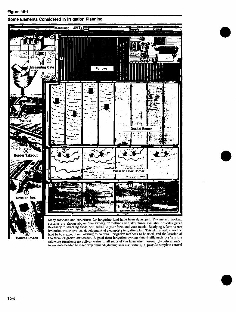
Fiaure 15-l
Some Elements Consldered in lrrigatlon Planning
Dlvlslon Box n
Basin or Level Border ~-, ,, “,,, ~--.
Many methods and structures for irrigating land have been developed. The more important systems are shown above. The variety of methods and structures available provides great flexibility in selecting those best suited to your farm and your needs. Readying a farm to use irrigation water involves development of a complete irrigation plan. This plan should show the land to be cleared, land leveling to be done, irrigation methods to be used, and the location of
Canvas Check the farm irrigation structures. A good farm irrigation system should efficiently perform the following functions: (a) deliver water to all parts of the farm when needed, (b) deliver water in amounts needed to meet crop demands during peak use periods, (c) provide complete control
154
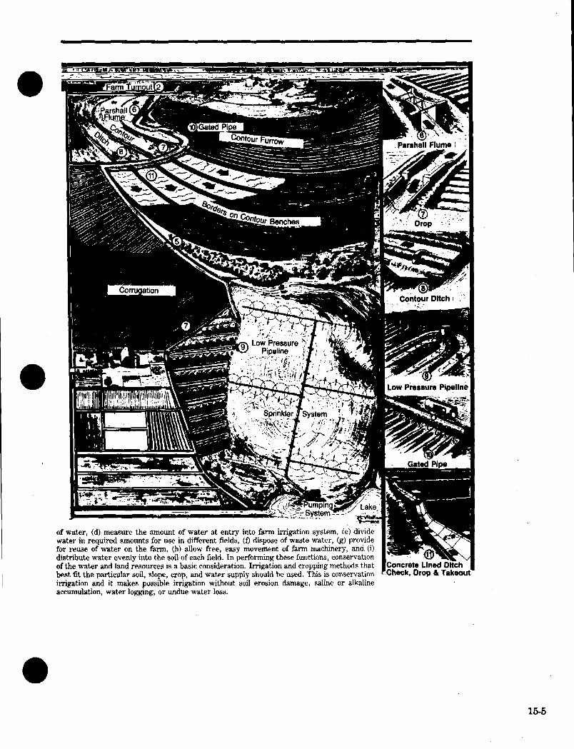
.-
of the water and land iesources is a basic consideratiin. Irrigazon and croppini methods that Concrete Lined Di6h best fit the particular soil, slope, crop, and water supply should be used. This is conservation 1 .Chak, DrOP & Takeout irrigation and it makes possible irrigation without soil erosion damage, saline or alkaline accumulation, water logging, or undue water loss.
15-5

the salts downward. In areas where the water quali- ty is not known, teBtB Bhould be made and evaluated by soil Bcientists or ether specialiBtB. The total concentration of Boluble salts, the relative pr@ portion of sodium to other cations, the preBence of toxic amounts of boron or other elements, and the relative concentration of bicarbonates to calcium and magnesium should be determined. l?acilitieB to test water quality are available through state agricultural collegeB, public health departments, and commercial 1aboratorieB.
Erosion Control and Drainage
The irrigation planner is faced with Bimultaneous- ly meeting the following three objectiveB: (1) apply water efficiently without causing eroBion, (2) protect against erosion CauBed by rainfall, and (3) provide required surface and subsurface drainage-
The physical layout requirementB for proper ir- rigation are often directly opposed to the phyBica1 requireients for protecting the land against eroBion by rainfall. This is especially true with surface methodB of irrigation. To protect a field against ero- sion caused by stormB, it is often deBirable to lay out the rows so the furrows are nearly level; however, for water application it may be easier to install a less efficient ByBtem by running the rows directly downslope. UBing contour irrigation with or without terraces and contour bench leveling to modify slope often satisfy both requirements. In other instances, conventional erosion control prac- tices are inBtalled and the irrigation water iB ap- plied by sprinklerB.
Si:!nilarly, the needs for drainage and irrigation are not necessarily compatible. On some soils it may be deBirable to apply irrigation water by pond- ing, such as by the use of level borders, but such a practice may not be compatible with the drainage requirement for removal of exCeBB storm water. On the other hand, land leveling for irrigation uBually helps the surface drainage of a field by eliminating small ponded areas.
The application of irrigation water may change the balance between recharge and discharge of the ground water, which may reBult in changeB in the elevation of the water table. Usually, when water is diverted from an outside source for application to an area, the water table riBes and may reach a point where subsurface drainage is required. When irrigation water is pumped from the water table,
15-6
the water table may drop. If subirrigation is the method used, BubBurface drainage must neceBBarily be of a controlled type.
When the planner haB met the requirementB for efficient irrigation, effective erosion control, and adequate surface and subsurface drainage, he or she has developed a plan that sets the framework for consewation irrigation by the farmer.
Farm and Ranch Enterprises
An investigation for planning an irrigated farm is not complete until the type of enterprise that the farmer planB to develop is known. The crops to be grown, the labor available, and the intenBity of the operation - all influence the layout. Although the irrigator may have an opinion regarding the beBt methods and layout, it is the job of the planner to BuggeBt alternativeB that will provide a Bound baBis fo* the final deciBion.
The irrigation plan deBcribeB major componentB of the irrigation system and their operation, It lists the basic soils, agronomic and engineering data aB they apply to the specific irrigated unit, and spells out in detail how irrigation water management is to be achieved.
Economics
The economics of irrigation must be conBidered during irrigation planning. The planner needs to show that the benetitB will be sugicient to juBtify the cost of purchaBing, installing, and operating the irrigation system and that there will be a reasonable return on time, labor, and investment.
The actual cost of the ByBtem and its installation must be estimated. This cost will vary greatly depending on the type of system, size and length of distribution lineB, water source, number and type of water control structures, and other significant field conditions. The cost of operation and maintenance needs to be included. ThiB cost may be annual power costs, water assessments, repair, mainte- nance, insurance, or taxes. Any additional crop pro- duction coBts should be estimated, and it may be wiBe to develop an annual sinking fund for future equipment replacement.
The returns or benefits to be accrued from irriga- tion should be estimated. They may consist of only the difference between the value of irrigated cropB
0 -

Ba8ic Design Criteti
and dryland crops. Or they may include such in- tangible items as ensuring a stabilized farm in- come, ensuring a feed supply for a livestock opera- tion, allowing an increp in the production of the farming operation without adding land, and increm ing the valu6 of tie land.
Dasign criteria for each irrigation method are con- tained iq state irrigation guides and the ap- propriate chapters in Section 16 of the SCS Na- tional Engineering Handbook. Design criteria for ir- rigation practices are found in the &ion ‘Tractice Standards and Spec&ations” in the SCS National Handbook of Conservation Practices, and in the local field office technical guide.
16-7
Irrigation Methods
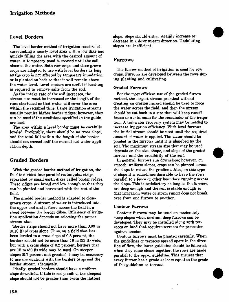
Level Borders
The level border method of irrigation consists of surrounding a nearly level area with a low dike and quickly filling the area with the desired amount of water. A temporary pond is created until the soil absorbs the water, Both row crops and close-grown crops are adapted to use with level borders as long as the crop is not affected by temporary inundation or is planted on beds so that it will remain above the water level. Level borders are useful if leaching is required to remove salts from the soil.
As the intake rate of the soil increases, the stream size must be increased or the length of the runs shortened so that water will cover the area within the required time. Large irrigation streams usually require higher border ridges; however, they can be used if the conditions specified in the guide are met,
The area within a level border must be carefully leveled. Preferably, there should be no cross slope, and the total fall within the length of the border should not exceed half the normal net water appli- cation depth.
Graded Borders
With the graded border method of irrigation, the field is divided into parallel rectangular strips separated by small earth dikes called border ridges. These ridges are broad and low enough so that they can be planted and harvested with the rest of the f&d.
The graded border method is adapted to close- grown crops. A stream of water is introduced into the upper end and it flows across the field in a sheet between the border dikes. Eficiency of irriga- tion application depends on selecting the proper stream size.
Border strips should not have more than 0.03 m (0.10 ft) of cross slope+ Thus, on a field that has been leveled to a cross slope of 0.3 percent, the borders should not be more than 10 m (33 ft) wide; but with a cross slope of 0.2 percent, borders that are 15 m (50 f’t] wide may be used. On steeper slopes (0.7 percent and greater) it may be necessary to use corrugations with the borders to spread the border stream adequ tely.
Ideally, graded bor I! ers should have a uniform slope downfield. If this is not possible, the steepest slope should not be greater than twice the flattest
15-8
slope. Slope should either steadily increase or 0 decrease in a downstream direction. Undulating slopes are ineffrcient.
Furrows
The furrow method of irrigation is used for row crops. Furrows are developed between the rows dur- ing planting and cultivating.
Graded F’urrows For the most efficient use of the graded furrow
method, the largest stream practical without creating an erosion hazard should be used to force the water across the field, and then the stream should be cut back to a size that will keep runoff losses to a minimum for the remainder of the irriga- tion. A tail-water recovery system may be needed to increase irrigation efficiency* With level furrows, the initial stream should be used until the required amount of water is applied. The water should be ponded in the furrows until it is absorbed by the soil. The maximum stream size that may be used depends on the size, shape, and slope of the graded furrows and the erodibility of the soil.
In general, furrows run downslope; however, on smooth, uniform slopes, crops can be planted across the slope to reduce the gradient. Also, on this type of slope it is sometimes desirable to have the rows parallel to a fence or other boundary running across the slope. This is satisfactory as long as the furrows are deep enough and the soil is stable enough so that irrigation water or storm runoff does not break over from one furrow to another.
conhur Furrows Contour furrows may be used on moderately
steep slopes when medium deep furrows can be developed+ They may be installed along with ter- races on land that requires terraces for protection against erosion.
Contour furrows must be planted carefully. When the guidelines or terraces spread apart in the direc- tion of flow, the lower guideline should be followed; when they come closer together, the rows are made parallel to the upper guideline. This ensures that every furrow has a grade at least equal to the grade of the guideline or terrace.
0

Corrugations
Corrugations are identical to furrows except that they are used with close-grown crops and may be spaced in accordance with the properties of the soil instead of the requirements of the crop.
Corrugations may be used with other methods to facilitate the spreading of water or to reduce crusting, They also are used between borders to ir- rigate a crop or to guide water to small ridges be- tween contour ditches. When corrugations are used in this manner, the system design is. based not on the specifications for corrugations but on the specifications for the methods they facilitate.
Contour Ditch
The contour ditch method is widely used for ir- rigating close-grown crops on steep slopes. Using this method, ditches are laid out across the slope on a slight grade. Water is released from the ditches by means of siphon tubes or openings in the ditch- bank. Plowing a furrow on the lower side of the graded contour ditch so that the soil is thrown against the lower bank is a simple improvement that allows more uniform distribution of flow and generally increases the efficiency of this method.
sprinkle
In sprinkle irrigation, water is sprayed into the air by means of perforat$ pipes or nozzles operated under pressure* Sprinkle systems can be classified as portable, solid-set, or self-propelled. There are many diBerent types of systems within each of these broad classifications. Each type has certain advantages, disadvantages, or application characteristics that af&ct its suitability for a par- ticular site. Most sprinkle systems are designed by manufacturer representatives or equipment dealer;. It is very important, therefore, that the buyer is aware of the capabilities and limitations of the systems under consideration. For the designer to develop an adequate system design that iits the water supply and site conditions, he or she must have such basic information as the water-holding capacity and intake characteristics of the soil, con- sumptive use requirements of the crops to be grown, soil erosion susceptibility, and needed conservation measures.
Other information that will be useful to the buyer and designer of a sprinkle system is found in Chapters 3 and 11, Section 15, SCS National Engineering Handbook, and in the irrigation guide and the field o&e technical guide.
Subirrigation
The subirrigation method requires special site conditions that permit control of the water table through regulation of water application and drainage. This method is most often used on land that has a high water table and where subsurface drainage is needed to remove ground water and pro- vide soil aeration. If a high water table is not in- herent, a layer of slowly permeable material, or some other barrier, must exist at a depth that will permit the buildup of an artiticial water table without excessive losses. Topography should be relatively flat and uniform. Soils must be deep enough to allow for any needed surface modification and to permit installation of the planned measures. Soil permeability must allow good vertical and horizontal movement of water.
A subirrigation system should apply water when irrigation is needed and remove water when drainage is required. Thus, an adequate irrigation water supply and an adequate drainage outlet must be available. The water conveyance and removal facilities may consist of (1) open ditches with water elevation control structures, (21 combination open channels and subs&ace drains and control struc- tures, or (31 buried pipelines, subsurface drains, and water control structures~
Each site is unique and requires special investiga- tions. System designs must be developed to meet the site conditions. Therefore, these operations should be carried out by personnel who have con- siderable experience with this irrigation method.
Trickle
Trickle irrigation is the slow application of water on or beneath the s&ace layer, usually aa drops, tiny streams, or miniature spray through emitters or applicators placed along a water delivery line. Trickle irrigation includes a number of methods or concepts, such as drip, bubbler, and spray irrigation.
15-9
Drip irrigation applies water tc the surface layer or below in discrete or continuous drops or in tiny streams through small openings. Often, the terms dr@and trickle irrigation are cousidered synony- mous. Discharge rates for widely spaced individual applicators are generally less than 20 L/hr (6 gal/b.r) and for closely spaced outlets along a tube (or porous tubing) sre generally less than 4 I&u (1 gal/hr) per foot of lateral or tube.
Bubbler iirigation applies water to the surface layer as a small stream or four&in from an open- ing having a point discharge rate greater than that for drip irrigation but generally less than 4 Unin Cl gal/minJ. The applicator discharge rate normally exceeds the infiltration rate of the soil, and a small basin is usually required to conbin or control the distribution of water.
Spray irrigation applies water tc the surface layer by a small spray or mist. Air is instrumenti in the distribution of water, whereas the soil is responsible in drip aud bubbler irrigation. Discharge rates are generally less than 115 Uhr (30 galihr).
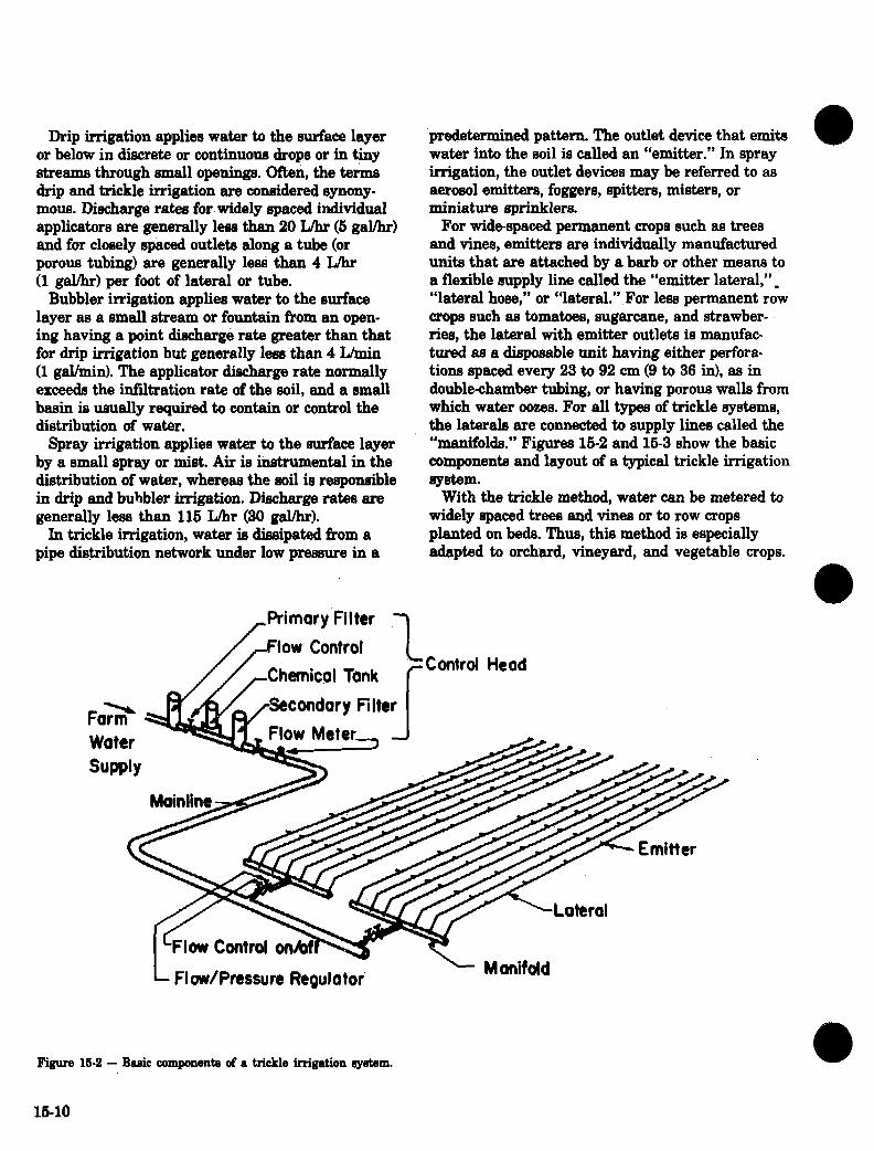
In trickle irrigation, water is dissipated from a pipe distribution network under low pressure in a
/
Primary Filter
-Flow Control
@redetermined pattern. The outlet device that emits water into the soil is called an “emitter.” In spray irrigation, the outlet devices may be referred to as aerosol emitt8rs, foggers, spitters, misters, or miniature sprinklers.
For widespaced permanent crops such as treea and vines, emitters are individually manufactured units that sre attached by a barb or other means to a flexible supply line called the “emitter lateral,“. “lateral hose,” or “lateral.” For less permanent row crops such as tcmatoss, sugarcane, and strawber- ries, the lateral with emitter outlets is manufac- tu& as a disposable unit having either perfora- tions spaced every 23 to 92 cm (9 to 36 in), as in doubleahamber tubing, or having porous walls from which water ooxes. For all types of trickle systems, the laterals are connected to supply lines called the “manifolds.” Figures 16-2 and 15-3 show the basic componenta and layout of a typical trickle irrigation system.
With the trickle method, wamr can he metered to widely spaced trees and vines or to row crops planted on beds. Thus, this method is especially adapted to orchard, vineyard, and vegetable crops
1 ‘Flcnv Cantrol on&w
Flow/Pressure ReQulotor M onifold
Figure 16-2 - Basic componenta of a trickle irrigation my&m.
15-10

a Labor costs and water use can be reduced with trickle-itigation because these systems need to be regulated rather than tended, and much of the sur- face layer is never wetted by irrigation water. Effl- cient control and placement of fertilizer can be ac-. complished with trickle systems. These systems can be designed to operate efficiently on almost any tvxrwb.
The main disadvantiges inherent in trickle irriga- tion systems are their comparatively high cost; susceptibility to clogging; their tendency ti build up local salinity; and, where improperly designed, their
Block
extremely partial and spotty distribution of soil moisture.
Trickle irrigation systems are normally designed and managed to apply light, frequent applications of water and to wet only part of the soil. Therefore, the procedures used to compute water requirements, irrigation depth and frequency, and salinity con- trols for other methods of irrigation must be ad- justed for trickle irrigation. For detailed informa- tion and design and evaluation procedures ap- plicable to trickle irrigation, refer to Chapter 7, Sec- tion 15, SCS NatiiSnal Engineering Handbook.
Manifold I
5 I
Mainline I
l Water Supply
II
, I and
I Cent rol Head
I I Block
-Laterals With
Emitters
-a---w.
h
Control V&es
IV
Figure 16-3-Typical two-shtiou, split-flow layout for a trickle irrigation ayetern with bloch I and LII, or II and IV operating aimultaneouely.

Water Conveyance
Capacity
Irrigation water must be conveyed from its source through a system of canals, pipelines, or structures to the individual furrow border or sprinkler head* For projects or group systems, a canal system usual- ly delivers the required flow to the farm headgate. The plan must provide conveyance from the headgate or farm source te the individual-field and furrow. The conveyance system must have the capacity to deliver to the field a flow that is ade- quate to meet the largest size of stream required for the irrigation methods planned for the field and to meet the consumptive use of the crops to be grown, making provisions for the expected field irrigation efficiency.
Some waste results when transporting the water from the headgate or pump to the field. If the water is carried in buried or surface pipelines, this loss may be negligible. In lined ditches the loss will also be very slight, depending upon the type of lining and its condition. Water conveyed in open, unlined ditches may have considerable loss, sometimes 15 to 40 percent per kilometer (25 to 66% percent per mile) or more on permeable soils. When unlined ditches are used, the farm requirement is equal to the field requirement plus the amount of the ditch losses.
Open Ditches
Some capacities and dimensions of permanent open ditches are given in exhibit 16-l. A ditch that will safely convey the required stream should be selected.
In designing a permanent ditch, a profile of the centerline, showing the location and elevation of the water supply and any required turnouts, cross- ings, drainage bypasses, and the like, is required. The water level at field turnout points must be high enough to provide the required flow onto the field surface. The water level required varies with the type of takeout structures, but the head should be at least 10 cm (4 in). &fer to Chapter 3, Section 15, SCS National Engineering Handbook for infor- mation on lined and unlined ditches.
Structures
In the selection of a specific structure, the depth of flow “d” should always equal the depth of flow-in the ditch, and the structure capacity should equal or exceed the design flow capacity of the ditch. Standard structure8 should be used wherever pos- sible. If a special design is required, the job should be designed in cooperation with someone having authority to approve it.
Criteria for certain types of irrigation structures are given in Chapter 6 of this manual. These criteria may be used to determine if a structure is adequate, even though it has not been built accord- ing to an SCS standard plan. In most instances it is desirable to exceed minimum requirements to provide longer life, better operation, or easier con- struction. Whenever possible, the farmers and con- tractors should be encouraged to utilize the stan- dard plans already available.
Drops
Drops are placed in a ditch or canal to hold the velocity of the flow within allowable limits, to in- crease the head on turnout devices, or both. Veloc- ity limitations for irrigation ditch and canal standards are described in the technical guide.
Drop structures should be placed so that, if need- ed, they can be used to divert water onto the land. A good rule to use for the location is to place the structure about 3.0 or 4.6 m (10 or 15 ft) downstream from the point where the water level is 0.15 m (0.50 ft) above the graded land surface. This procedure appears to place the structures on fill; however, since the line represents the water level and not the ditch bottom, the structure will always be on firm ground.
The height of drop structures used to lower water from one control point to another should be based on the economics involved and the desires of the farmer. Since two smaller drops take more materials and labor than one larger structure, the tendency in newly irrigated areas is to use fewer, higher drops.and keep the cost down. In many of the older irrigated areas, the tendency is to use more small drops to eliminate deep ditches between structures. For small farm ditches the height of the drop in meters should not exceed 0.3 times the land slope in percentage. A drop more than 1 m (3 ft) high should seldom be used. With large streams
-
15-12

this height is sometimes increasad. On steep slopes it is often advisable to use a concrete-lined ditoh section or pipeline to lower the water.
Turnouts should be placed so that it is not necessary to check the water above the design flow of the ditch, thereby providing a safety factor if water is turned down the ditch with the check flashboards still in place.
Crossings should be provided so that equipment will have access -to all parts of the field. With pipe drop structures, a crossing can be provided by ex- tending the length of the barrel and increasing the width of the fill.
Pipelines
Irrigation pipelines can be used for the same pur- poses as open channels or in place of open channels, Because the pipelines almost eliminate losses from evaporation and seepage, water distribution effi- ciency is high. They are particularly adapted to areas where seepage losses from ditches are high. Pipelines have an advantage over open ditches, where it is difficult to excavate and where it is necessary to carry water down steep slopes. Buried
pipelines do not require as much land as ditches; therefore, the land can be used for other purposes. Pipelines require careful planning for correct loca- tion, capacity requirements, proper selection of materials, and construction methods. Ccnerally, the services of an engineer are required. Chapter 3, Sec- tion 15, SCS National Engineering Handbook, gives further information on pipelines.
Measuring Devices
Measuring devices are needed so that the farmer knows how much water he or she is using and can make the necessary adjustments for efficiency. The simplest of all measuring devices is a weir, but it requires a loss of head to function accurately. When such a head loss cannot be tolerated, a Parshall flume or trapezoidal flume may be used. Many large ditch companies have measuring devices built into the headgates. Some pumping installations are equipped with flowmeters on the discharge line. Ap propriate measuring devices should be considered as essential items for good irrigation water manage- ment. See Section 15, Chapter 9, of the SCS National Engineering Handbook for further information.
15-13

Land Leveling Water Disposal System
For more efficient application of irrigation water by surface method.8, it is often nece88ary to modify the topography. Such modification, made according to a blan providing for specific elevation8 at each, point, is called land leveling.
The relief clas8es for surface-irrigated land are ahown in exhibit 16-2. If the surface relief meet8 the 8tandard8 for cla88 D or E, only @or or very poor irrigation water efflcienciea are po88ible, and leveling ia required for con8ervation irrigation. The ideal land am-face for aurface irrigation ha8 little or no croaa alope and haa a uniform domeld alope that ia alight enough that erosion from rainfall and irrigation water ia not a problem and adequate enough to provide good aurface drainage. If the con- ditiona are appropriate, the ideal land aurface ia flat in both direction8. The alope limitation8 vary from location to location becau8e of difference8 in aoil and rainfall.
Some field8 are ideal, requiring no leveling. Generally, however, it ia neceaw to do 8ome level- ing on each field. Standard8 for aati8factory leveling have risen over the yeara and farmera are deciding that it i8, worthwhile to relevel some field8. Many irrigation areaa that are being leveled to a “C” claaa relief probably will eventually be leveled to “B” or even “A” claaa relief. For this rea8on, the planner should design the beat job the farmer can afYord. Detail8 for designing, ataking, and leveling land are given in the SCS National Engineering Handbook, Section 15, Chapter 12.
A complete water diapoaai &tern should be planned for each irrigated farm. This diapoaal 8yatem 8hould be able to convey storm and irriga- tion ruuoff to an outlet without catming exceaaive ero8ion. It should be incorporated aa part of the drainage design on land8 that require or have a aubaurface drainage ay8tem. On land8 that require only 8urface water diapoaal, the drainage ayatem 8hould be built at the same time the land8 are leveled, if po88ible.
In many case8 the di8po8al system will use water- ways designed principally to catty storm runoff, If irrigation tail water i8 to enter these waterwaya, special planting8 and maintenance often muat be 8pecifid.
a -
a I 15-14
Equipment
In addition to sprinkle systems, the farmer has a wide choice of portable irrigation equipment. This portable equipment has been developed to permit more accurate distribution of water and to reduce labor requirements,
Check Dams
Several types of canvas, plastic, and metal check dams sre available for both lined and unlined ditches; These check dams are designed to block the flow in a ditch just below the point where the water is to be turned out. They can be placed at any loca- tion and are not in the way when aditch needs to be cleaned or rebuilt. Most check dams are ad- justable so that the water can be held at some con- stant level.
Siphon Tubes
Siphon tubes are widely used to withdraw water from an imigation ditch. They range from 1 cm (0.4 in) in diameter to large fabricated siphons that carry as much as 57 IJs (15 gal/s). The small tubes usually are used for furrow irrigation, although a number of them may be used together for border or contour ditch irrigation.
For furrow irrigation, the tube sizes usually are selected so that two or three tubes per furrow will deliver the maximum stream recommended for the slope being irrigated. .After the water has crossed the field, one tube is removed tc provide the “cut- back” stream. The approximate dischsrge of small aluminum siphon tubes is given in exhibit 15-3. The head shown is the difference in height in the supply ditch and the centerline of the discharge end of the tube or the water level in the furrow when the dischsrge end is submerged.
Gated F%pe
Gated pipe is made of lightweight metal or plastic and has small gates or openings spaced to match the fmows The pipe comes in sections that sre easy for one person to handle and is fitted with simple watertight connections. A alightly different product made of vinylcoated glass, cloth, butyl, plastic, or canvas hose and equipped with small outlets can be used for the same purpese. Gatecl
pipe reduces water losses during conveyance and provides a positive control of the water to each individual furrow. Cperating heads of more than 0.0 m (2.0 ftl usually require ‘&socks” on the open- ing to avoid erosion.
Computing the head loss in a reach of gated pipe with the gates closed is similar to computing it for any similar pipe. For the. reach in which the gates are open, the friction is first computed as if the en- tire flow were carried the full length. The computed value is then multiplied by a factor which depends on the number of outlets. This factor is given in ex- hibit 15-4.
Some head is required at the last gate to produce flow through the gate. The head required depends on the type of gate used and the desired flow. Usually the head is less than 0.3 m (1.0 ftl.
An example of a calculation on gated pipe follows. Assume that the flow of water needed is 63 L/s (17 gal/s) through a 2O-cm (8-m) gated pipe 396 m (1,300 I%) long, and that 0.31 L/s (0.10 gal/s) must flow through each of the last 200 gates. Gates are spaced 1 m (3 ft) apart.
What is the total head loss if a 2O-cm @-in) pipe has a friction loss of 2.47 m per 100 m (2.47 ft per 100 ftl for a flow of 63 L/s (17 gal/s)?
Given: Num&r of gates 200 Multiple gate factor (exhibit 15-4) 0.33 Length of pipe with gates open 204 m (670 ft) Length of pipe with gates closed 192 m (630 ft)
Solution: Gpen line loss (2.04 ml x 2-47 x 0.33= 1.66 m
K6.70 IV x 2.47 x 0.33 = 6.40 ftl
Closed line loss (1.92 ml x 2.47 = 4.74 m K6.30 ft) x 2.47 = 15.60 ftl
Total loss C 6.40 m (21.00 ftJ
15-15
Methods of Measuring or Estimating Soil Moisture
To determine the required depth of irrigation water to be applied at any given time, the irrigator should fast estimate or measure the amount of available moisture in the soil within the root zone depth. There are several methods of doing this. Ad- ditional information on the advantages and limita- tions of these methods are given in the SCS Na- tional Engineering Handbook, Section 15, Chapter L
Soil sampling and drying. This method involves sampling each type of soil in the field at desired depths and at several locations. The soil samples are weighed, dried, and weighed again. The dif- ference in weight is equal to the weight of the moisture. Usually this is expressed as a percentage of the weight of the dry soil.
Tensiometer. The tensiometer consists essentially of a porous cup filled with water and connected by a continuous water column to a vacuum measuring device, either a gage or manometer. Thti cup is buried in the soil at the desired depth and measurements are read above ground on the vacuum indicator. This instrument measures soil moisture tension directly. A moisttie characteristic curve for the particular soil being irrigated is re- quired to convert moisture tension measurements into percentage of available moisture in the soil.
Electrical instruments. Electrical instruments operate on the principle that achange in moisture content produ,ces changes in some electrical proper- ty of the soil or of an instrument inserted in the soil. In most cases this property is electrical conduc- tivity. Electrodes are permanently mounted in con- ductivity units. These units are usually blocks made of nylon, Fiberglas, or gypsum. These blocks are buried at the desired depth, and changes in the moisture content of the soil are reflected by changes in the electrical resistance in the blocks. Resistance or conductance meters are used to measure the resistance. It is necessary to calibrate the blocks in the iield by comparing the resistance readings with the soil moisture contents determined by over&y- ing samples taken from the same relative position as the blocks.
Gas pressure instruments. Instruments such as the csrbide moisture tester utilize the principle of chemical drying of the soil sample, A reagent such as calcium carbide is mixed with the moist soil sam- ple within a sealed chamber. The chemical reaction
16-16
of the reagent and the soil moisture produces acetylene gas. The gas pressure registers on a gage that is calibrated to indicate the wet weight . moisture percentage of the soil. Convenient tables are available to convert these values to dry weight moisture percentages. The reaction and readings normally require about 3 min per sample.
Feel and appearance meth&d. This method is rather widely used to estimate the amount of available moisture in the soil. Samples are taken from various depths and at several locations in the field. A soil sampling tube, auger, or post-hole dig ger is used, The feel and appearance of the samples are compared with a table, or a guide such as ex- hibit 154, and the soil moisture level is thus estimated. With practice and experience the ir- rigator should be able to estimate the moisture level within 10 to 16 percent.
Evaporation pan method. This method uses the relationship of crop consumptive use to the evapora- tion from standard evaporation pans. Evaporation pan data are approximations of consumptive use and are not measurements of soil moisture. The amount of soil moisture usedin a given period must be calculated. This calculation is made by applying a factor to the crop that is to be irrigated to the depth at which water evaporated from the pan dur- ing that period. This calculated amount then represents the soil moisture used by the crop.
Moisture accounting method. Consumptive use values are used to maintain a daily inventory of the remaining soil moisture. Starting at a time when the moisture level in the soil is known, a “book- keeping” system is set up whereby the computed consumptive use is subtracted daily from the record- ed available moisture in the soil. Rainfall and ir- rigation amounts are added to the motiture balance when received. The success of this method depends on accurate measurements of the water-holding capacity of the soil, determination of daily consump- tive use rates, and measurement of rainfall and ir- rigation amounti.

Irrigation Water Management
0
l
Introduction
Irrigation water management practice8 8re the timing and regulating of irrigation water applica- tiona 80 that the water requirement8 of the crop are 8ati8fied without wasting water or lOSing aoil. Water ia, applied in amounta that can be held in the soil for crop need8 and at ratea that do not cause runoff and erosion.
The irrigator provide8 the management, not the structure. For example, an irrigator may in8tall a headgate to control the flow of water onto a field. The headgate itself provide8 no water management. The water ia managed when the irrigator open8 the gate to deliver water to the field or clo8ea the gate to atop delivery. Before irrigating, the irrigator mu8t decide, for example, when to open the gate, how far it should be opened, and when it should be clo8ed. The ability to make sound water manage- ment deciaion8 ia the moat important aspect of con8ervation irrigation water management.
To make sound deciaion8, the irrigator mu8t understand the ba8ic principle8 involved. He or ahe muat have a general idea of how water ia held in the 8oil for plant u8e and how much water the 8oil hold8. The irrigator needs to know how to judge when irrigation ia needed and how much is needed. He or ahe should have a general understanding of aoil intake characteriatic8 and of the required ad- ju8tment.8 in atream aize8 and time of water applica- tion according to the intake rate8 of the aoila.
bgarding irrigation water management, the main objective8 of SCS are to give farmera an under8tanding of conservation irrigation principle8 show them how to judge the etfectiveneaa of their own irrigation practice8 and help them make needed adjuatmenta in old ayatema or in8tall new ayatema. The rest of this chapter provides guidance in meeting these objectivea.
Basic Soil-Moisture-F’lant Relationships
Available Water Capacity An irrigater muat under&and the u8able water
capacity of 8oila. Lack of this knowledge generally result8 in overirrigation and wasted water.
When a aoil i8 irrigated, water moves down through the void8 or openings between 8oil par- ticles, forming a film around each individual 8oil grain. This film ia held tightly around the aoil
graina when amall amount8 of water are available. When the amount of water increaaea, the film become8 thicker and the aurface tension deCrea8e8. When the film becomea a0 thick that the am-face tension will no longer reaiat the pull of gravity, the extra water movea through the aoil. The amount of water held around the soil graina again8t the pull of gravity i8 called the “field capacity” of the aoil. This ia the moisture condition of a well-drained aoil a day or two after a thorough irrigation or rain.
Aa planti use water from the aoil, the tilm around the 8oil grains becomes thinner and more tightly held. When the film become8 a0 thin that plants can no longer pull the water from around the 8oil graina, the aoil ia aaid to be at the “wilting point.” Available water capacity of a 8oil ia the amount of water that can be held between the limit8 of field capacity and wilting point.
While it may not be important that irrigator8 know how water ia held in the aoil for plant use, it ia important that they know how much can be held and that there ia a limit to the available moiature- holding capacity of each aoil.
For irrigation, it ia convenient to think of the available water capacity of aoila aa the depth of water in millimeter8 per millimeter (inches per inch) of soil depth. The moisture held in any given 8oil profile or crop root zone ia the summation of the amount8 held in each 0.3-m (14%) increment of the total depth.
Many determination8 of the available water capacity .of 8oila have been made. The available Water Capacity Of some 8Oil8 i8 ahown in irrigation guides that have been prepared for apecifrc irriga- tion area8 For tho8e aoils not covered in the irriga- tion guides the available water capacity can be estimated by u8ing table 15-l.
1517
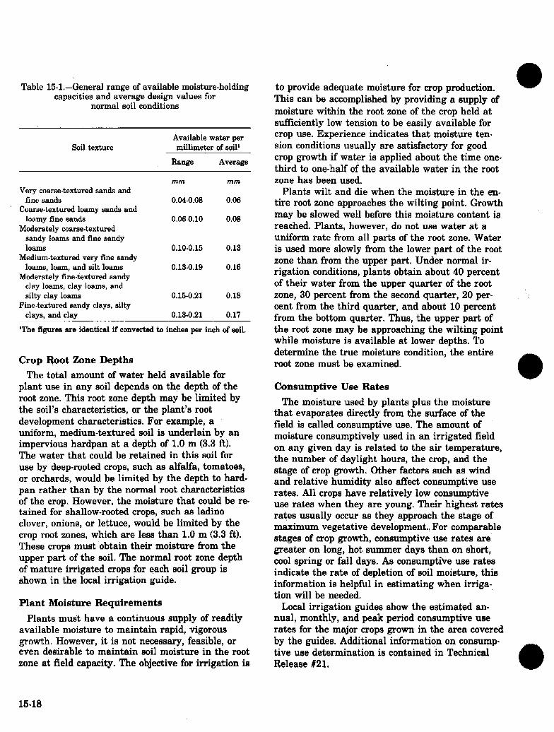
Table 15-l.-General range of available moisture-holding capacities and average design values for
normal soil conditions
Soil texture Available water per millimeter of soil1
Range Average
mm lnm Very coarse-textured sands and
fine sands 0.04-0.08 0.06 Coarse-textured loamy sanda and
loamy fine sands 0.060.10 0.08 Moderately coarse-textured
sandy loams and fme sandy loams 0.10-0.16 0.13
Medium-textured very fine sandy loams, loam, and silt loams 0.13-0.19 0.16
Moderately fme-textured sandy clay loams, clay loama, and silty clay loams 0.15-0.21 0.18
Fine-textured sandy clays, silty clays, and clay 0.13-0.21 0.17
The figurea are identical if convertad to inches per inch of soil.
Crop l$oot Zone Depths The total amount of water held available for
plant use in any soil depends on the depth of the root zone. This root zone depth may be limited by the soil’s characteristics, or the plant’s root development characteristics. For example, a uniform, medium-textured soil is underlain by an impervious hardpan at a depth of 1.0 m (3.3 ft). The water that could be retained in this soil for use by deep-rooted crops, such as alfalfa, tomatoes, or orchards, would be limited by the depth to hard- pan rather than by the normal root characteristics of the crop. However, the moisture that could be re- tained for shallow-rooted crops, such as ladino clover, onions, or lettuce, would be limited by the crop root zones, which are less than 1.0 m (3.3 ft). These crops must .obtain their moisture from the upper part of the soil. The normal root zone depth of mature irrigated crops for each soil group is shown in the local irrigation guide.
FYant Moisture Fbquirements Plants must have a continuous supply of readily
available moisture to maintain rapid, vigorous growth. However, it is not necessary, feasible, or even desirable to maintain soil moisture in the root zone at tield capacity. The objective for irrigation is
16-18
to provide adequate moisture for crop production. This can be accomplished by providing a supply of moisture within the root zone of the crop held at sufliciently low tension to be easily available for crop use. Experience indicates that moisture ten- sion conditions usually are satisfactory for good crop growth if water is applied about the time one- third to one-half of the available water in the root zone has been used.
Plants wilt and die when the moisture in the en- tire root zone approaches the wilting point. Growth may be slowed well before this moisture content is reached. Plants, however, do not use water at a uniform rate from all parts of the root zone. Water is used more slowly from the lower part of the root zone than from the upper part. Under normal ir- rigation conditions, plants obtain about 40 percent of their water from the upper quarter of the root zone, 30 percent from the second quarter, 20 per- cent from the third quarter, and about 10 percent from the bottom quarter. Thus, the upper part of the root zone may be approaching the wilting point while moisture is available at lower depths. To determine the true moisture condition, the entire root zone must be examined.
Consumptive Use Fbtes The moisture used by plants plus the moisture
that evaporates directly from the surface of the field is called consumptive use. The amount of moisture consumptively used in an irrigated field on any given day is related to the air temperature, the number of daylight hours, the crop, and the stage of crop growth. Other factors such as wind and relative humidity also afYect consumptive use rates, All crops have relatively low consumptive use rates when they are young. Their highest rates rates usually occur as they approach the stage of maximum vegetative development. For comparable stages of crop growth, consumptive use rates are. greater on long, hot summer days than on short, cool spring or fall days. As consumptive use rates indicate the rate of depletion of soil moisture, this information is helpful in estimating when irriga- tion will be needed.
Local irrigation guides show the estimated an- nual, monthly, and peak period consumptive use rates for the major crops grown in the area covered by the guides. Additional information on consump tive use determination is contained in Technical Release #21.
a Evaluation Procedure
The effectiveness of a farmer’s irrigation water management practices can be determined from a few simple field observations. No matter which ir- rigation method is used, certain principles apply.
1. Water should be applied when needed to maintain favorable soil moisture conditions for good crop growth.
2. The amount of water applied should be sti- cient to reach field capacity in the root zone but should not greatly exceed this requirement. An ex- ception to this may be in humid areas when a soil moisture deiicit is planned to accommodate an- ticipated rainfall.
3. Water should be applied at a rate that does not cause significant waste or soil erosion.
An examination of a farmer’s irrigation water management practices should answer the following questions:
1. Is irrigation needed? 2. What is the soil moisture deficiency? 3. How much water is being applied? 4. Is irrigation causing erosion? 5. How uniformly is the applied water spread
over the tield? 6. How much of the water is imiltrated into the
soil? The first two questions are interrelated. A
knowledge of the soil moisture deficiency (amount of water needed to refill the root zone to iield capacity) is necessary to determine whether irriga- tion is needed. Therefore, they may properly be considered together.
Need for Irrigation arid Amount to Apply The amount of moisture remaining in the root
zone and the need for irrigation may be determined by using any of the instruments or methods described previously under the heading of “MethcKls of Measuring or Estimating Soil Moisture.”
The soil moisture deficiency also. can be estimated roughly from a knowledge of the pattern of consumptive use by the particular crop, if the number of days since the last irrigation is known. For example, in an area where the irrigation guide indicates that the peak period consumptive use rate of a particular crop is about 0.8 cm (0.3 in) per day during a hot dry period, the average soil moisture deficiency would be about 8 cm (3 in) some 8 or 10 days after the last irrigation.
During periods of more moderate weather condi- tions, the moisture deficiency would not be ex- petted to be so great. These kinds of estimates can- not be precise, but they are useful in checking the reasonableness of the estimates made by the soil sampling procedure outlined earlier.
The question, “Is irrigation needed?“, cannot always be answered precisely. Most crops should be irrigated before more than about half of the available moisture in the crop root zone has been used.
Some crops are thought to do better at higher moisture levels. (less moisture deficiency at time of irrigation). Therefore, irrigation may be needed well before half of the available water has been used. Generally, one may consider that the need for irrigation is doubtful for any crop until the soil moisture deficiency approaches one-third of the available moisture+holding capacity of the crop root zone. Special-purpose irrigations, such as for seed germination, are exceptions to this general rule.
Most crops have a critical growth period during which a high moisture level must be maintained to obtain high-quality yields. This critical period generally is during the blooming or fruiting stage.
In determining the need for irrigation, the possibility that some parts of the field may be drier than other parts should not be overlooked. Sometimes, because of poor distribution of irriga- tion water, the soil moisture deficiency is con- siderably greater in one part of the field than in another part. A@ the soil in one part of the field may have a lower available water capacity than the soils in another part. The moisture in one soil might be depleted to the 50-percent level long before the other soils approach that level. If such critical areas are of significant size, the decision to irrigate should be based on the available water in the drier areas.
Amount Applied
The amount of water required to refill the root zone (net irrigation requirement) usually is expressed in centimeters of depth. For ease in making comparisons, the amount of water actually delivered onto the field should be calculated in the same terms.
Irrigation water deliveries usually are calculated in terms of the rate of flow. The commonly used units of flow are liters per second (L/s) and cubic meters pr second (ma/s). The miner’s inch (M.I.) is an old flow unit that is still used in some Western
15-19
States. It is the quantity of water that will flow through an orifice 1 ins under stated head, which varies from 4 to 6% in. in different localities. Another unit sometimes used is million gallons per day bgdl.
Rate of flow is a volume delivered in a given timo interval. If a time interval is specified, flow units can be converted to volume units. For exam- ple, a flow of 1 ft% (flow rate) for 1 hr (time inter- val) will deliver 3,600 ft? (volume) of water* If this volume is spread evenly over an area of 1 acre (43,560 ft3), the depth will be 0.083 ft (36,000/ 43,560), and the volume would be 0.083 acre-f%. This volume is equal to 0.083 x 12 = O-99 acre-in. For practical use in the field, the volume can be considered to be 1 acre-in.
The above conversion of flow rate to volume is the basis for a handy formula that sheuld be known and well understood by all irrigators and irrigation technicians:
28 L/s for 1 hr = 1 ha-cm (1 fP/s for 1 hr = 1 acre-in
If flows are measured in cubic feet per second, gallons per minute, miner’s inches, or million gallons per day, they can be converted, to equivalent liters per second by using the following approximate relationships:
28 L/s = 1 ft?ls = 450 galfmin = 38.4 MI. in Colorado = 40 M.I. in Arizona, Montana, Nevada,
northern California, and Oregon = 50 M.I. in Idaho, Kansas, Nebraska
New Mexico, North Dakota, South Dakota, southern California, Utah, and Washington
= 0.65 mgd = 0.028 ma/s
After the volume of water delivered.onto a field has b&en computed in terms of hectare-centimeters (acre-inches),, it is a simple matter to calculate the equivalent average depth throughout the fmld. Divide the hectare-centimeters (acre-inches) by the number of hectares (acres) covered, Thus, 5 ha-cm (5 acre-inches) spread over an 0.8-ha (2 acre) field is equal to an average application depth of 6.3 cm (2.5 in)., or
15-20
d (cm) = Q (ha-cm) (per F) X !I’ (hr)
d (in) = Q @‘/a) or acre-in (per hr) X !I’ (hr) A (acre)
Three variables must be known to compute the average depth of water applied on a field (1) the size of the irrigation stream, (2) the time water & run onto the field, and (3) the area of the field. These variables do not consider the surface outflow. The following examples illustrate the computation procedure:
Example 1
Given:
Stream size = 112 L/s (4 ftVs) Irrigating time = 10 llr Field area = 3.2 ha (8 acres)
Find the average depth applied:
Solution:
(Metric) (English)
28 L/s for 1 hr = 1 ftVs for 1 hr = 1 ha-cm 1 acre-in
28 L/s for 10 hr = 1 ftVs for 10 hr = 10 ha-cm 10 acre-in
112 L/s for 10 hr = 4 W/s for 10 hr = 40 ha-cm 40 acre-in
40 ha-cm
3.2 ha = 12.5 cm applied
40 acre-in 8 acres
= 5 in, applied
Example 2
Given:
Stream size Irrigating time Field length Field width
= 24 L/s (375 gal/min) = 12 hr = 201 m (660 ft) = 50 m (16s ft)

Find the average centimeters (inches) depth applied
Solution:
= 24 cm applied
= 9.6 in. applied
(Metric) (English)
24 L/s for 1 hr = 0.84 ha-cm
24 L/s for 12 hr = 10 ha-cm
201 m x 50 m = 10,050 ma
10,050 ma/lO~OOO = lha
10 ha-cm
1 ha
10 acre-in 2.5 acres
Example 3
Given
Stream size
Irrigating time Field length Furrow spacing
3?5 gialhlliIl/450 = 0.84 ft’la
0.84 fWs for 1 hr = 0.84 acre-in
0.84 fta/s for 12 hr = 10 acre-in
660 ft x 165 ft = 108,900 W
108,900 W/43,560 = 2.5 acres
= 10 cm applied
= 4.0 in. applied
= 68 L/min (18 gal/mid (average per furrow)
= 24 hr = 442 m (1,450 ft) = 0.91 m (3 ft.1
Find the average depth applied
Solution:
(Metric) (English)
68 Llminl6Os = 1.13 us
1.13 L/s for 1 hr = 0.04 haem
1.13 L/s for 24 hr = 0.96 haall
442 m x 0.914 m = 404 ma
404 mVlO,OOO = 0.04 ha
18 gal/min/450 = 0.04 ftvs
0.04 W/s for 1 hr = 0.04 acre-in
0.04 ftVs for !24 hr = 0.96 acre-in
1,450 ft x 3 ft. = 4,350 ft’
4,350 ftV43,560 = 0.1 acre
0.96 ha- 0.04 ha
0.96 acre-in 0.1 acre
Example 4
Given:
Stream size = 21 L/min (5.5 gal/min) (average per sprinkler)
Irrigating time = 11*5 hr Lateral spacing ~=, 15.24 m (50 ft) Sprinkler spacing = 9.15 m (30 ft)
Find the average inches of depth applied:
Solution:
(Metric) (English)
21 L/mm/60 = 5.5 galJminl450 = 0.35 L/e 0.012 w/s
0.35 L/s for 1 hr = 0.012 W/s for 1 hr = 0.012 ha-cm 0.012 acre-in
0.36 Ids for 11.5 hr = 0.012 ftVs for 11.5 hr = 0.138 harm 0.138 acre-in
15.24 m x 9.14 m = 50 ft x 30 ft = 139 ma 1,500 ft’
139 m*/10,000 = 1,600 W/43,560 = 0.014 ha 0*034 acre
0.138 ha+zm 0.014 ha
= 10 cm applied
0.138 acre-in 0.034 acre
= 4 in. applied
ln all of the examples where the flow rate is given in terms of liters per second (gallons per minute), the general form of the equation for depth (d) in centimeters (inches) is as follows:
d km) = flow (L/s) x time (hours) x
28 x length (m) x width Cm) 10,000 rns
15-21

d (in) = flow (gal/min) x time (hours) X
450 x length (feet) x width (feet) 43,560
d (cm) = flow (L/a) x time (hours) x 10,000 length (m) x width (m) x 28
C flow (L/s) x time (hours) x 357.14 length (m) x width (m)
d (in) = flow (gal/mm) x time
(hours) x 43,S60 length (feet) x width (feet) x 450
C flow (gal/min) x time (hours) x 96,8 length (feet)’ x width (feet)
Since 28 L/s flowing 1 hr is not exactly 1 ha-cm, the above equation for d is not exact. For exact conversions, the factor 357.14 shown above should be 357.7. The conversion equation is usually shown as:
d (cm) = sprinkler discharge (L/s) x
hours x 357.7 lateral spacing (m) x sprinkler spacing (m)
d (in) = sprinkler discharge (gal/min) x
hours x 96.3 lateral spacing 6%) x sprinkler spacing (ft)
Thus, for Example 4, the depth applied would be computed as:
d (cm) = 0.35 X 11.5 X 357.7 c 10 cm 15.24 x 9.14
d (in) = 5.6 x 11.5 x 96.3 = 4 in 50 x 30
Since lateral spacing multiplied by sprinkler spacing is just another way of saying length multiplied by width (equals area), the sprinkler conversion equation can be used for all situations where the flow rate is given in terms of liters per second (gallons per minute). Example 2 can be used as an illustration.
IS-22
d (cm) = 24 x 12 x 357.7 = 10 cm 20 x 50
d (in) = 375 x 12 x 96.3 = 4 in 660 x 165
In furrow irrigation work, the rate of flow as measured in individual furrows often is convertid to average depth as follows:
d (cm) = L/m flow per 100 m of furrow length x hours
furrow spacing in meters
d (in) = gal/min flow per 100 ft of furrow
length x hours furrow spacing in feet
This is equivalent to:
d (cm) L/min x hours x 6 length (m) x width (m) (or spacing)
d (in) = gal/min x hours x 100 length x width (or spacing)
While this is less accurate than the other conver- sion methods discussed, the error is slightly less than 4 percent,
Field Application Effuziency
The field application efficiency is determined by dividing the net amount of water needed to refill the root zone by the amount of water actually ap- plied onto the field. Thus, if the net amount of water needed is 8.1 cm (3.2 in) and the amount ap plied is 12.7 cm (5.0 in), the field efficiency is 64 percent (8.1 crnA2.7 cm = 0.64 or 3.2 inl5.0 in = 0.64).
High efficiency does not always mean good irriga- tion. The water may not have been distributed evenly over the field, or the amount applied may not have been enough to bring the root zone up to field capacity. On the other hand, low field efliciency usually means poor use of water and indicates a need for a careful check of the water management practices being used.
No clear distinction exists between high and low efficiencies. It is impossible to irrigate at an efli- ciency of 100 percent. Yet, the further irrigation

a
departs from this ideal, the more costly it becomes from the standpoint of water use and the more apt it is to damage the soil. In general, all water ap plications should be made at the highest efficiency level that is practical a.nd feasible. State irrigation guides give the percent efficiency that the average irrigator, can expect to obtain if good management practices are used in a properly designed and developed system.
Uniformity of Application
Adequate irrigation refills the planned root zone storage capacityLthroughout the field. To do this with a minimum amount of loss to deep percola- tion, the water must spread uniformly over the field so that each part of the field will have the same opportunity time to take in water* Oppor- tunity time is the length of time that irrigation water is available at the surface for infiltration in- to the root zone.
The best way to determine whether a field has received adequate irrigation is to check the soil moisture conditions a day or so atter irrigating. Dig or auger into the soil at representative loca- tions to see if the root zone haa been brought up te field capacity. If dry layers or areaa are found, irrigation was not complete or the water was not spread evenly.
For surface methods of irrigation, the uniformity of water distribution can be checked by determin- ing how long the water is on the surface at various points along the length of the run. If this length of time is about the same at all p.oints and the soils are similar, it can be assumed that the same amount of water has int?ltrated the soil in each part of the field. Usually, a check on the opportu- nity time at all points along the length of the run can be determined by obseting the time water reaches and recedes from selected points. These data are used to plot advance and recession curves as shown in figures 154 and 4A. The vertical distance between the advance curve and the reces- sion curve at any point along the length of the run is the “intake opportunity time” at that point. The opportunity time & all pointa should be sufGcient to permit the desired amount of water to infiltrate the soil.
Water didribution in furrows. Since the volume of water contained in a furrow as temporary sur- face storage at the end of irrigation usually is relatively small, furrow recession curves are nearly
flat. In other words, the water stops flowing z lower end of the furrow within a few minutes the water is turned off (figures E-4 and 4AX Therefore, to obtain good water distribution, 1 “advance” period should be as short as possil
Flaure 15-4
Sample Advance and Recession Cur\ Time (min.)
Furrow mk jbcession curve
400
300
Advance curve
Time (min.)
Border
400 Recession curve
300
200
100
0 0 50 100 200 250
Distance (m)
Figures 154 and 4A show an irrigation tha meets the above criterion. In this example ar take opportunity time of 340 min is required the desired amount of water into the soil. Op tunity time at any point along the furrow is time between the advance and recession curv tcok 85 min for the furrow stream to reach tl of the run. The water was turned off 410 mir the start of irrigation and stopped flowing in lower end of the furrow 16 min later.
The required intake opportunity time is sht the broken line drawn parallel to the advanc curve. The shaded area above the broken linl
it the I after
the pie.
/es
!
min.
10
i
min.
300
1t 1 in- to put Npor- the ‘e8. It he end Iafter the
mm by e 2
E-23
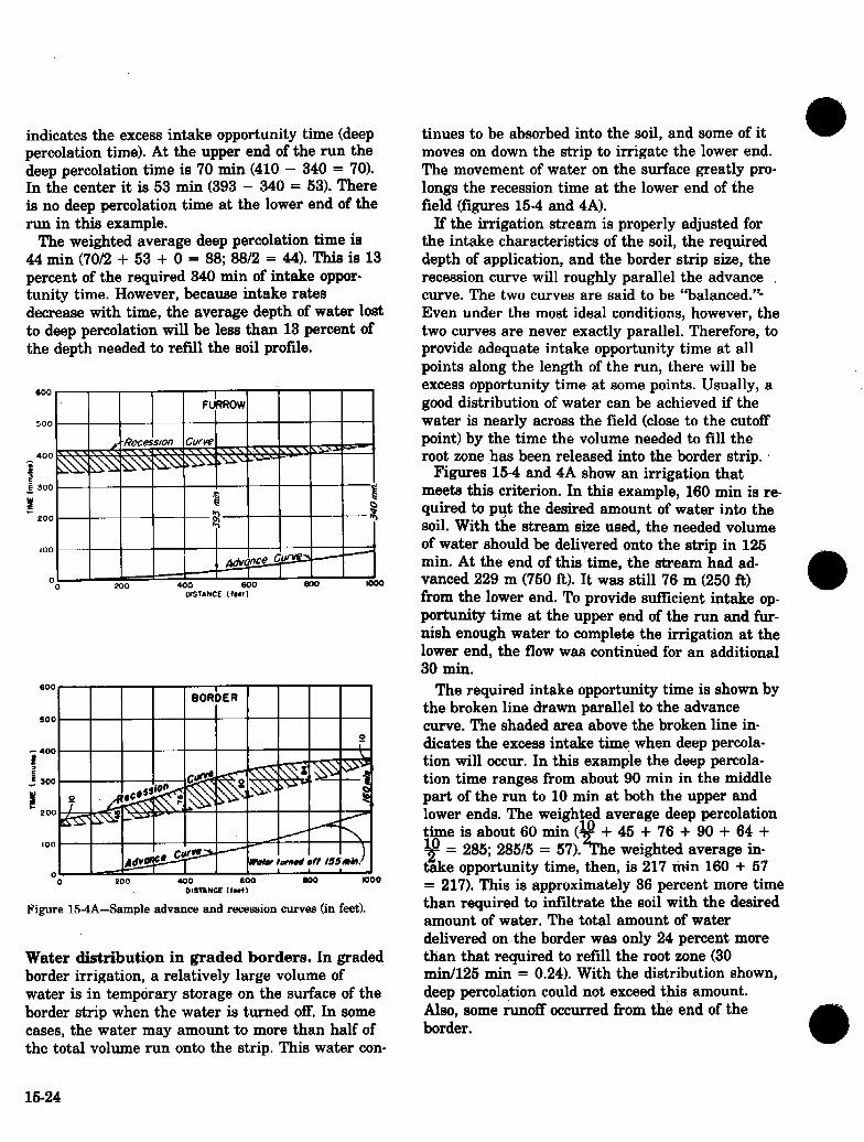
indicates the excess intake opportunity time (deep percolation time). At the upper end of the run the deep percolation time is 70 min (410 - 340 = 70). In the center it is 53 min (393 - 340 = 53). There is tie deep percolation time at the lower end of the run in this example.
The weighted average deep percolation time is 44 min (70/2 + 53 + 0 = 88; 8812 = 44). This is 13 percent of the required 340 min of intake oppor- tunity time. However, because intake rates decrease with time, the average depth of water lost to deep percolation will be less than 13 percent of the depth needed to refill the soil profile.
6DO
5DO
400 < 2 1 300
: I- 200
IO0
0 0
600
500
- A00
! 2 3OD
g I- ZOD
I00
0 0 *oo 4DO 600 600 moo
Figure 15-4A-Sample advance and receseion curven (in feet).
Water diskibution in graded borders. In graded border irrigation, a relatively large volume of water is in temporary storage on the surface of the border strip when the water is turned off, In some cases, the water may amount to more than half of the total volume run onto the strip. This water con-
tinues to be absorbed into the soil, and some of it moves on down the strip to irrigate the lower end+ The movement of water on the surface greatly pro- longs the recession time at the lower end of ihe field (figures 15-4 and 4A).
If the irrigation stream is properly adjusted for the intake characteristics of the soil, the required depth of application, and the border strip size, the recession curve will roughly parallel the advance curve. The two curves are said to be “balanced.“- Even under the most ideal conditions, however, the two curves are never exactly parallel. Therefore, to provide adequate intake opportunity time at all points along the length of the run, there will be excess opportunity time at some points. Usually, a good distribution of water can be achieved if the water is nearly across the field (close to the cutoff point) by the time the volume needed to fill the root zone ,has been released into the border strip.
Figures 15-4 and 4A show an irrigation that meeta this criterion. In this example, 160 min is re- quired to p$ the desired amount of water into the soil. With the stream size used, the needed volume of water should be delivered onto the strip in 125 mine At the end of this time, the stream had ad- vanced 229 m (750 ft). It was still 76 m (250 ft) from the lower end. To provide sticient intake op- portuniw time at the upper end of the run and fur- nish enough water to complete the irrigation at the lower end* the flow was contimied for an additional 30 min.
The required intake opportunity time is shown by the broken line drawn parallel to the advance curve- The shaded area above the broken line in- dicates the excess intake tim!, when deep percola- tion will occur. In this example the deep percola- tion time ranges from about 90 min in the middle part of the run to 10 min at both the upper and lower ends. The weighted average deep percolation time is, about 60 min (’ + 45 + 76 + 90 + 64 +
Y = 285; 28515 = %h 57). e weighted average in- take opportunity time, then, is 217 tin 160 + 67 = 217). This is approximately 36 percent more time than required to intJltrate the soil with the desired amount of water. The total amount of water delivered on,the border was only 24 percent more than that required to refill the root zone (30 min/l26 min = 0.24). With the distribution shown, deep percolation could not exceed this amount. Also, some runoff occurred from the end of the border.
a -
15-24
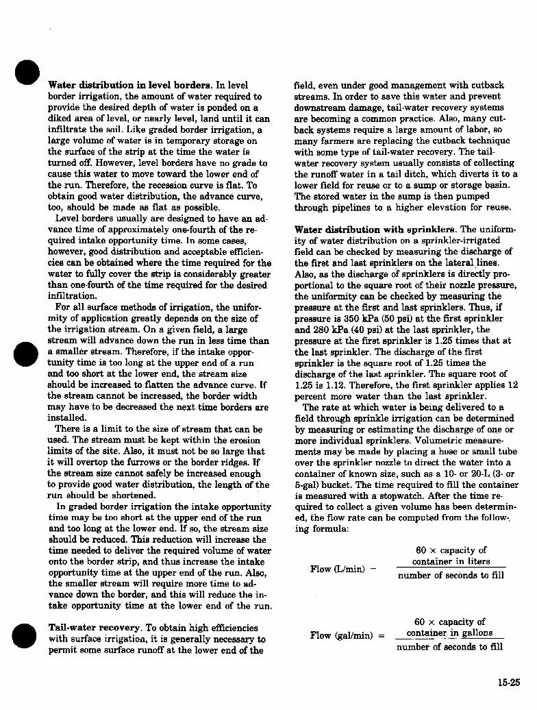
Water distribution in level borders, In level field, even under good management with cutbi border irrigation, the amount of water required to streams. In order to save this water and preve provide the desired depth of water is ponded on a downstream damage, tail-water recovery syste diked area of level, or nearly level, land until it can are becoming a common practice. Also, many f itiltrate the soil. Like graded border irrigation, a back systems require a large amount of labor, large volume of water is in temporary storage on many farmers are replacing the cutback techn the surface of the strip at the time the water is with some type of tail-water recovery. The tail turned OR. However, level borders have no grade to water recovery system usually consists of tolls cause this water to move toward the lower end of the runoff water in a tail ditch, which diverts the run. Therefore, the recession curve is flat, To lower field for reuse or to a sump or storage bj obtain good water distribution, the advance curve, The stored water in the sump is then pumped too, should be made as flat as possible. through pipelines to a higher elevation for rd
Level borders usually are designed to have an ad- vance time of approximately one-fourth of the re- quired intake opportunity time. In some cases, however, good distribution and acceptable efficien- cies can be obtained where the time required for the water te fully cover the strip is considerably greater than one-fourth of the time required for the desired imiltration.
For all surface methods of irrigation, the unifor- mity of application greatly depends on the size of the irrigation stream. On a given field, a large stream will advance down the run in less time than a smaller stream. Therefore, if the intake oppor- tunity time is too long at the upper end of a run and too short at the lower end, the stream size should be increased to flatten the advance curve. If the stream cannot be increased, the border width may have to be decreased the next time borders are installed.
There is a limit to the size of stream that can be used. The stream must be kept within the erosion limits of the site. Also, it must not be so large that it will overtop the furrows or the border ridges. If the stream size cannot safely be increased enough to provide good water distribution, the length of the run should be shortened.
In graded border irrigation the intake oppotiunity time may be too short at the upper end of the run and too long at the lower end. If so, the stream size should be reduced. This reduction will increase the time needed to deliver the required volume of water onto the border strip, and thus increase the intake opportunity time at the upper end of the run. Also, the smaller stream will require more time to ad- vance down the border, and this will reduce the in- take opportunity time at the lower end of the run.
Water distribution with tsprinklem. The un ity of water distribution on a sprinkler-irrigat field can be checked by measuring the dischar the fast and last sprinklers on the lateral,line Also, as the discharge of sprinklers is directly portional to the square root of their nozzle pre the uniformity can be checked by measuring t pressure at the first and last sprinklers. Thus, pressure is 350 kF’a (50 psi) at the first sprink and 280 Wa (40 psi) at the last sprinkler, the pressure at the fast sprinkler is 1.25 times th the last sprinkler. The discharge of the first sprinkler is the square root of 1.26 times the discharge of the last sprinkler. The square roa 1.25 is 1.12. Therefore, the fast sprinkler appl percent more water than the last sprinkler.
The rate at which water is being delivered t tield through sprinkle irrigation can be deters by measuring or estimating the discharge of o more individual sprinklers. Volumetric measu ments may be made by placing a hose or smal over the sprinkler nozzle to direct the water ii container of known size, such as a lo- or 20-L S-gal) bucket. The time required to till the con is measured with a stopwatch. After the time quired to collect a given volume has been dete ed, the flow rate can be computed from the fol ing formula:
Flow (L/mm) =
60 x capacity of container in liters
number of seconds to
Tail-water recovery. To obtain high efficiencies with surface irrigation, it is generally necessary to permit some surface runoff at the lower end of the
60 x capacity of Flow Cgal/min) = container in gallon
number of seconds to !

Thus, if 33 seconds are required to fill a 10-L (3-gal) bucket, the flow rate is 18.2 L/min. (5.4 gal/min).
ho x 10 Q= 33
= 18.2 L/min
60 x 3 Q= T =5.4 gal/min
Since sprinkler-nozzle discharge is relat&l to the pressure head at the nozzle, the flow rate can be reasonably estimated if the pressure is known. Most sprinkler manufacturers’ catalogs contain tables showing the discharge of their sprinklers as related to pressure. For reliable estimates the pressure must be measured at or close to the nozzle.
In some instances it may be feasible to determine the discharge of each sprinkler on a lateral. The values should be averaged to determine the average rate of application. One way of doing this is to measure the discharge of the fmst and last sprinkler on the lateral. The average discharge for all the sprinklers can then be computed as the discharge of the last sprinkler plus one-fourth of the difference between the first and last sprinklers.
Sometimes, because of topographic conditions, the minimum pressure may not be at the last sprinkler. If the sprinkler lateral runs downslope, the minimum pressure may be at the first sprinkler. Where sprinkler laterals are not laid out on a near- ly uniform grade, the pressure or discharge should be measured at the high and low spots as well as at the end sprinklers.
The volumetric measurements will indicate the overall distribution of water across the field, The uniformity of water distribution in the effective area of an individual sprinkler can be best deter- mined by setting out a pattern of catch cans and measuring the depth of water caught. The cans should be set in a symmetrical pattern across the lateral between two sprinklers. The cans should be about 1.5 m (5 ft) apart where’the sprinklers’ spac- ing is less than 9 m (30 ft), Three-meter (lo-ft,) spac- ing is adequate where sprinklers are 9 m (30 .ft,) or more apart. The procedure for making water distribution pattern tests is explained in Agricultural Handbook No. 82, “Methods for Evaluating Irrigation Systems.”
Usually, there is little need for making a distribu- tion patteti test unless soil moisture testi after an irrigation or the appearance of the crop indicate8 uneven water distribution, If sprinkler spacing and nozzle pressures meet the criteria given in Chapter 11, Section 15, of the National Engineering Hand-
book, distribution patterns usually will be satisfactory,
Water distribution in trickle systems. Since trickle systems are normally designed to wet only ,a part of the plant rooting area, it is very imporant. that they be checked periodically for adequate water application and distribution. Performance is evaluated by gathering and analyzing data on such items as (1) duration, frequency, and sequence of ir- rigation cycle; (2) moisture deficits in the wetted area; (3) rate of discharge and pressure at selected emission points; (4) changes in emission discharge rates with time; (5) percentage of soil volume wet- te& (6) location and uniformity of emission points ,with respect to the plants; and (7) losses of pressure at fdters. The procedure for making field evalua- tions of trickle systems is given in Chapter 7, Sec- tion 15, National Engineering Handbook.
Water distribution in center-pivot systems. Center-pivot systems are unique because the speed and the rate of water #application must increase as the distance from the pivot increases. This increase is accomplished by increasing the size of sprinkler nozzles, decreasing the spacing of sprinklers, or both. Therefore, there is no set application rate for these systems. If they are designed, installed, and operated properly, the depth of application will be nearly uniform over the length of the systems.
The operating characteristics of these types of systems can be checked by determining the gross application and application rate at a point toward the outside end of the lateral. The application rate will decrease toward the pivot and, therefore, will be satisfactory if the application rate at the outer end is within the soil intake capabilities.
The water distribution along the length of a center-pivot system can be checked by setting a line of evenly spaced measuring cans (or gages) ahead of the system, allowing the system to move over them, and measuring the depth of water caught in each can. If the depths measured are uniform, the average of all measured depths represents the amount applied to the field per revolution. If the depths of water caught differ widely, especially be- tween the inner and outer parts of the system, the average depth applied will need to be calculated us- ing weighted measurements. This can be done by assigning factors to multiply each measurement by, depending on the distance of the can from the pivot. If the cans are evenly spaced, use a factor of one (1)
a 15-26

for the fust can, two (2) for the second can, three (3) for the third can, and so on. Total the results of these multiplications.and divide by the sum of the can numbers (1 + 2 + 3, etc.) to obtain the average depth applied to the field per revolution of the Bystem.
Irrigation with sprinkle and level border or level furrow methods often produces no runoff. In such cases the average depth of water afiplied onto the tield is also the average depth that itiltrates the soil. When surface runoff does occur, however, it must be measured to determine the depth of water retained on the field.
The average depth of water that intiltrates the soil during irrigation can be best determined by subtracting the volume of water lost through sur- face runoff from the total volume applied t.e the field. This volume divided by the area of the field will be the average depth of water inChrated,
On many fields, surface runoff rates can be measured periodically in existing drainage or waste-water ditches to furnish adequate data for the computation of runoff volume. Where site conditions make it infeasible to collect and measure runoff from an entire field, measurements of runoff ratea from representative individual furrow or border strips may be used in estimating total runoff.
Runoff rates usually increase as intake rates decrease. Therefore, to determine the volume of sur- face runoff, the rate of runoff usually must be measured at intervals throughout the runoff period. Runoff rates are converted to runoff volumes by use of the conversion formula: 28 L/s flowing 1 hr equals 1 ha4m (1 IV/s flowing 1 hr equals 1 acre- in). The procedure is the same as explained previously for computing the amount of water ap- plied to the field. With changing flow rates, however, the comput&,ion must be made in steps. The volumes of runoff ere computed for each time interval between measurementi and summed to determine the total runoff. Table 15-2 shows a sam- ple set of runoff calculations. In this example, the rate of flow onto the field is assumed to be 42 L/s MI i%Vs) tbroughout the 12&r irrigation period+ The total volume run onto the field, therefore, is 18 ha-cm (18 acre-in).
If a field is irrigated by surface flooding, using bordera, basins, or contour ditches, cylinder in- filtrometers can be med to determine the amount of water that intiltrates the soil in a given pried. Figures 15-S and 5A show an intake curve developed from cylinder imiltrometer data.
In order to usecylinder intake curves as a basis for estimating the average depth of water that in- filtrates the soil, the average intake opportunity time must be known. For example, if the sample intake curve shown in figures 15-5 and 5A were developed on a bordered field that has the advance and recession characteristics illustrated by figures 15-4 and 4A, the average intake opportunity time would be 217 min (170/2 + 205 + 236 + 250 + 224 + 17012 + 1085; 108515 = 217). The weighted average depth of water that itiltrated the soil would be 12.5 cm (5 in).
Figures 15-4 and 4A for borders also show a minimum intake opportunity time of 170 min, which, according to the intake curve, is more than sufficient to have 10 cm (4 in) of water itiltrate the soil. Assuming this is the depth of water needed to refill the soil profile, the average.deep percolation loss would be 2.5 cm 0.0 in).
In a field irrigated by furrows or corrugations, the average depth of water that infiltrates the soil can be estimated from a measurement of the instan- taneous furrow intake rate. To use this procedure, the furrow intake rate should be determined by inflow-outflow measurements of individual furrows or of a group of furrows. The measurements should be made near the end of the irrigation period, generally sometime in the last quarter of the period. The difference between the inflow rate and the outflow rate will represent the rate of furrow in- take. The furrow intake rate should be expressed in terms of liters per minute per 100 m of furrow (gallons per minute per 100 ft of furrow). It can then be converted to an equivalent field intake rate, in centimeters per hour (inches per hour), by dividing by the furrow spacing, in meters (feet).
The field intake rate thus determined can be con- sidered the instantaneous rate at the end of the ir- rigation. The rate usually changes very little dur- ing the last part of the irrigation period, so any er- ror resulting from this assumption will be small. The average intake rate for the total irrigation, however, will include an initial period of relatively high intake rate which gradually diminishes to the instantaneous rate measured at the end of the ir- rigation. The difference usually will be greatest on fine-textured soils that characteristically have steep intake rate curves and least on coarse-textured soils that generally have relatively flat intake rate curves. For most soils the average rate can be ap- proximated by multiplying the final rate by the ap- plicable soil factor indicated in table 15-3.
15-27
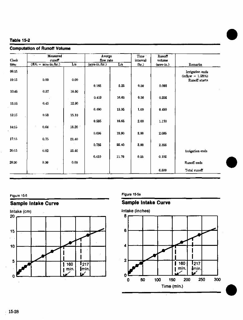
Table 15-2
Computatlon of Runoff Volume
Cklck time
08:15
10:15
IO:45
11:15
12zl5
14zl5
lFl5
2&15
20:30
0.00
0.37
0.46
0.53
0.64
0.75
OS2
0.00
Memured runoff
(ft% = acre-inhr.) L/S
0.00
10.50
12.80
15.10
18.20
21.40
23.40
0.00
J-
Averge
0.135 5.25
0.410 16.66
0.4W 13.96
0.595 16.65
0.696
0.785
0.410
19$0
22.40
11.70
flow rite (acre-in./hr.) Us
Time Runoff intervaI volume
(hr.1 (acre-in.)
0.60
0.50
1.09
2.00
3-00
3.09
0.25
--
0.093
0.205
0.490
1.170
2,085
2.355
0.102
6.500 Total runoff
Remarks
Irrigation ends (inflow = 1.5ft%)
Runoff starts
Irrigation ends
Runoff ends
Fiaure 15-5 Figure 155a
‘Sample Intake Curve Sample Intake Curve
Intake (cm) Intake (inches) 20
15 h
10
5
0
4 I i I A- 217
l&7. I
0 50 100 150 200 250 300 Time (mine)
I 15-28

Table 15.3-Soil factora for estimating average intake rate from final intake rate ’
Soil texture Soil factor
Fine and moderately fine clays and clay loams
Medium and moderately coarse Bilt loams t.& sandy loama
Coarse and very coarse loamy sands and sands
1.60
1.33
1.20
The average intake rate multiplied by the average intake opportunity time will equal the average depth of itiltration
The computations umd to estimate the average depth of infrltration (d) were derived from meuurementa of the instantaneous rate of intake and are illustrated in the following example:
Assume: Estimathqj Rates of Flbw
Moderately coarse- textured soil (factor = 1.33)
Furrow Bpacing = 0.91 m (3.0 ft) Total irrigating time = 8.0 hr Average intake
0pportuniQ time = 6.9 hr
Intake rate measurementa made on three representative furrow sections about 7 houm after start of irrigation.
Measurementa and computations:
(Metric) Furrow number 1 2 3
Inflow rate Sta. 0 + 00 - Unin 77.0 80*5 74.0
Outflow rate Sta. 0 + 61 - L/min 66.0 67.3 63J
Intake rate - L/mm 11.0 13.2 11.7
Average 12.
d (cm) 12 x 6.9 x 6 = x 1.33 = 12 cm 61 x 0.91
(English) Furrow numb 1 2
Inflow rate Sta. 0 + 00 - gal/rain
Outflow rate Sta. 2 + 00 - gal/mm
Intake rate - gal/mm
20.4 21.3 l!
17.4 17.8 11
3.0 3.5 , Average 3.2.
3.2i2.0 = 1.6 gal/r&i per 100 ft final furrow rate,
1.60/3.0 = 0.533 in. per hour final field rate. 0.533 x 1.33 = O-71 in. per hour average tie1
rate 0.71 x 6.9 = 4.9 in. average intake depth.
The d&u&on and examples preBented to illus- trate procedure8 for evaluating irrigation water management practicea have a@sumed that the rat of flow of the tiigation stream was known. In many cases this is true. If water is delivered fron well, the farmer usually knows the approximate discharge. Many irrigation districts and irrigatio: companies measure delivev f’hw~ at the farm headgate. &me farm system8 have weir8 or other water-measuring device5 ti measure the flows to
specific fields. If the rate8 of flow are not known, however, it may be necessary to rely on estimate; Measurements of some kind usually are needed. $ome of the most usable estimating procedures, such as the float method and velocity head rod fo open channel8 and the trajectory method for pipe flow, are discussed in Chapter 3 of thiB manual a Chapter 9,. Section 16, SCS National Engineering Handbook.
Soil Erosion
Erosion is a hazard on most irrigated lands. Ar irrigation method that causes a significant amou of erosion cannot be considered satisfactory.
Serious erosion can occur even when little or n soil iB removed from the field. Where surface irri tion iB used, the irrigation streams are largest where they fnet enter the field. As they progr@Ba toward the lower end of the field, the streams arj reduced by the amount of water infiltrated into t
l!

soil. Often the large streams will erode the soil at the.upper end of the field but have insufficient car- rying capacity at the lower end to remove the material from the field.
Soils irrigated by a surface method usually have the greatest erosion during the initial stages of ir- rigation. The dry surface soil, sometimes loosened by cultivation, is readily moved by the flowing water. After a short period of soaking, however, the soil settles and becomes more diEcult to move. Us- ing sprinkle irrigation, however, the erosion pattern is apt to be reversed. At the start of irrigation, the intake rate may be higher than the application rate so no runoff or erosion will occur. In the later stages of irrigation, however, the intake rate m&y become less than the application rate. If this occurs, the water may begin to move over the surface and cause erosion. Sprinklers should be designed and operated so that the application rate does not ex- ceed the soil intake rate.
With surface irrigation, some soil movement can be expected. However, irrigation streams should not be so large that they cut furrow side slopes, form rills in border strips, or cause other obvious move- ment of soil toward or off the lower, end of the tield. Even though irrigation streams can be controlled to prevent erosion, measures may be needed to control erosion caused by rainfall, as discussed in the sec- tion “Relationship to Erosion Control and Drainage.”
Special Problems
When evaluating irrigation water management practices, it is important that all of the circum- stances, conditions, and objectives involved be carefully examined. Under some conditions the con- servation use of water resources cannot be ap praised adequately in terms of a computed field ap plication efficiency. It may be,necessary to evaluate the whole farm or, in some cases, an entire irriga- tion project or watershed area. Also, there are con- ditions under which a needed irrigation cannot be applied without substantial deep percolation or sur- face runoff. If the water is reused on the same or adjacent field and the water quality is not impaired, the surface runoff may not be undesirable. Some of the more commonly encountered problems are dis- cussed in subsequent sections.
15-30
Irrigation at High Moisture Levela
Sometimes it is necessary to apply irrigation water when only the top few inches of soil are below field capacity. This kind of irrigation may be needed to:
1. Supply moisture for seed germination, 2. Keep the surface moist to prevent crusting on
some soils, or .
3. Wet the surface to reduce damage to emerg- ing plants caused by salt accumulations.
Using surface methods of water application for such light irrigations may be very ineficient. Where only one such irrigation is needed to get a crop established, the low level of efficiency usually can be tolerated. The use of sprinklers should be considered, however, if several of these light irriga- tions are required. Lettuce growers in the Salinas Valley of California, for example, have found that by irrigating with sprinklers until thinning time, they can greatly reduce the amount of water needed and at the same time obtain a more uniform crop stand. After thinning time, the crop is irrigated by the furrow method. In other areas farmers have noticed distinct advantages in using sprinklers to establish grass and legume crops.
Evaluation studies of these early season, special- purpose irrigations are desirable. These studies, however, usually form a poor basis for appraising the farmer’s overall irrigation water management practices since irrigation systems usually are designed for normal irrigation required after the crops have become established.
LAmal Spread of Water
Furrow spacing usually is fixed for cultivated row crops. On these fields, irrigation must be continued until an adequate lateral spread of water has been obtained. On some soils, the extended time needed for adequate wetting between furrows may result in a low application efficiency. The entire ground sur- face need not be wetted (“blacked out”) in most cases. Usually, however, irrigation should be con- tinued until the wetted bulbs from adjacent furrows touch, or nearly touch, at their widest point. Very little lateral spread can be expected after the water is turned OR most of the moisture movement or soil drainage will be vertical.
The problem of obtaining adequate lateral spread usually is greatest with crops planted on high ridges or beds. l% is especially hard to obtain ade- quate lateral spread if there are also steep irriga- tion grades that limit the depth of flow in the fur-
@
-
rows. Improvements often can be made by changing the irrigation layout to irrigate across the slope. The flatter irrigation grade8 will permit the use of furrow streams that have greater depths of flow and greater wetted perimeter8. Sometime8 it is even desirable to use level furrows. The increa5ed wetted area will reduce the distance that the water has to move laterally and upward into the beds, Sometimes the lateral movement can be speeded by rolling or otherwi8e compacting the beds. Loose ridges or beds often have many large pore spaces. When the beds are compacted, pore size distribution is improved and capillary movement is accelerated.
hdillg In 5ome areas, extra water is needed to prevent
the accumulation of exce8sive amount5 of salts in the crop root 5one. The process of removing these 8alts by the action of percolating water is called leaching. Leaching can be effective only if drainage through the root zone is possible.
Water for leaching should be applied according to a plauned program. Usually, extra water for leaching need not be applied at every irrigation. Generally, a satisfactory salt balance can be main- tained by making leaching applications during the nonpeak irrigation period, A need for leaching is never an adequate excuse for poor irrigation water management practices. Ineflicient and poorly distributed irrigation water applications are more apt to intensify salt problems than to alleviate them. After a soil has been drained and initially leached, the amount of’excess irrigation water ap- plied to maintain a favorable salt balance should be based on the quality of the water and the salt tolerance of the crops being irrigated. This deter- mination require8 detailed analysis and 8hould be made only by those thoroughly familiar with the leaching process.
of the irrigation run8 will have nearly a8 much in- take opportunity time as the upper ends, The farmer stop5 irrigating when the water has been ap plied long enough tc refill the crop root zone but makes no effort to minimize 8urfac.e runoff. Runoff i8 collected in waste water ditche8 and returned to the stream. Field application efficiencies may average les8 than 50 percent; however, there i8 no waste of the water re8ources The surface runoff is immediately returned to the stream channel where it is available for diver8ion by downstream users. There is no 5Oil erO8iOn, and Water lo88e8 from deep percolation are minimized.
Situations 8uch as that described should be fully considered in evaluating a farmer’s irrigation water management practices. Always, however, one must be 5ure all of the pertinent factors are taken into account. Water qualiw, for example, is a factor sometimes overlooked. Irrigation water lost through deep percolation often is recovered in the stream a8 return flow. Seldom, however, is this water com- parable in quality tc the original stream supply. Percolating waters usually pick up some salts as they move through the 8oil profile. Return flows from surface runoff may also be lower in quality under some circum8tances. Water management practices that result in low field application efficien- cies, therefore, should be examined thoroughly before they are accepted a8 meeting con8ervation objectives.
Overall Water Resource Use A primaiy objective of the Soil Conservation Ser-
vice i8 to conseive the u8e of water. conservation of water, however, i8 not alway synonymous with high field application efficiency. There are cir- cumstances in which applying irrigation water at very low efficiency is ju8tified.
Suppose, for example, a farmer in the upper part of a watershed has a water supply available for diver8ion that far exceeds the consumptive needs of the crops. Water is spread over the field8 u8ing large but. nonerosive stream8 80 that the lower ends

Moisture Accountihg Method for Scheduling Irrigation
Use
Moisture accounting is a proven useful method for scheduling irrigations in humid areas by pro- viding a running account of available moisture in the effective root zone. It requires a daily recording of rainfall, estimated evapotranspiration, net irriga- tion amounts, and moisture balance methods that depend upon the accuracy with which available moisture-holding capacities of the soil, rainfall, net irrigation amounts, and evapotranspiration values are determined. The same degree.of accuracy should be used in determining each of these factors. Therefore, use of the method is limited to those areas where reliable values can be obtained. In humid areas, occasional rains refill the root zone to field capacity, thereby preventing an accumulation of errors that might tiect the accuracy of the method.
Of all the factors mentioned in the previous paragraph, perhaps the most critical to determine is daily evapotranspiration. Values of this factor must be reliable, yet relatively simple to determine by the average irrigator. A compromise is required be- tween accuracy and the practical limitations im- posed by field conditions.
In the Northeastern United States the relation- ship of evapotranspiration to daily hours of sun- shine and stage of crop growth has been satisfac- torily established. Generalized tables are available that provide daily adjustments to evapotranspira- tion based on observations of sunshine hours. New tables and different adjustment factors, or possibly an entirely new kind of estimating procedure, will be needed in other areas of the United States.
Basic F’rinciples
The moisture accounting method is based on two principles:
1. When an adequate supply of available moisture is present in the effective root zone, the rate of consumptive use by a given crop depends primarily on the stage of growth and climatological conditions.
2. When the moisture content of the effective root zone is known at any given time, the moisture content at any later time can be computed by crediting moisture gained from effective rainfall or
irrigation and subtracting the daily moisture withdriwals during the elapsed time.
Conditions for Use
To apply the basic principles, the following are necessary:
1. Soils with good internal and surface drainage.
2. An adequate irrigation system and water suPPlY*
3. Daily consumptive use values for the crop. 4. Sticient plant population, 5. Accurate total available moisture values. 6. A k,nowledge of the effective root zone of the
crop. 7. Measurement of effective rainfall and irriga-
tion applications at the site. 8. Occasional soil moisture checks to verify the
account, especially during the critical periods of crop growth and for inexperienced users.
Equipment mquired
1. Wedge-shaped plastic rain gage with a SO- by 62.5-mm (2- by 2%in) minimum top opening.
2. Record book. 3. Means of measuring average application rate
of sprinklers or the application amount by surface methods.
Installation and Reading of the Rain Gage
The rain gage should be set on a post lmated in the field or in an open area adjacent to the field be- ing irrigated. The distance of the gage from nearby obstructions that might affect the catch, such as trees or buildings, should be at least twice the height of the obstruction. The gage should be about 1 m (3 ft) above ground level and its top should be at least 8 cm (3 in) above the top of the post.
The amount of rainfall in the gage should be read at the lowest point of the water surface. The reading should be made as accurately as possible. After the rainfall amount has been record&d, the gage should be emptied and reset in ita holder.
15-32

‘Use of the Moisture Balance Sheet for Scheduling Irrigation
A moisture balance sheet for scheduling irrigation is shown in tables 154 and 4A. Although the exam- ple is for a crop of early potatoes, the same pro- cedure applies to other crops and soils. The example is from an account for an entire growing season. The overall procedure for using the balance sheet is as follows:
1. Record all available pertinent information in the heading. (See table 15-4 or 4A.1
2. Determine the total available moisture- holding capacity- of the effective root zone and record it in the heading of the form. Use one of the following sources:
a. Field testing. Field-measured values of moisture percentage at field capacity and wilting point should be used whenever possible. !l’he moisture percentage at wilting point should be taken from soil characteristic reports on represen- tative soils or estimated as described later in the section “Moisture Percentage at Wilting Point.”
b. Irrigation guides. c. Other publications giving characteristics
of local soils. 3. Determine the balance when irrigation is to
begin. The value frequently used is 50 percent of the total available moisture in the effective root zone, but the value should be selected to suit site conditions and the operational plan. Irrigation must begin when the soil moisture is at a level that will permit the completion of the irrigation cycle before the available moisture is seriously depleted. Some farmers may desire a starting balance that provides for the maintenance of moisture above 50 percent. Others may choose a starting balance that permits irrigation applications of a stated amount, that is, about a 2&m (l-in) net irrigation at each application.
Beginning Moisture Balance On a date near the normal planting date or start
of growth for perennial crops and tree fruits, when the field is at field capaci@, enter the total available moisture-holding capacity of the soil in the daily balance column (6) of the Moisture Balance Sheet (see table 154 or 4A).
1. If the moisture percentage at field capacity has been determined previously for the field, measure the current moisture percentige to provide
an accurate value for starting the moisture balance sheet
2. If no field measurement of moisture percent- age at field capacity is available, begin the account with an estimated value. At the first opportunity after adequate rain or irrigation obtain the field capacity moisture percentage and correct the ac- count accordingly.
3. If at the time of plant emergence, a week or more has passed since the soil was at field capacity and tillage and seeding operations have ensued, estimate the moisture balance as being about 1.3 cm (0.5 in) below the field capacity value.
4. Estimate early season moisture losses before plant emergence by using an evaporation rate from the soil surface at 0.08 cm (0.03 in) per day for the fast week after the soil has been wetted to field capaciw. Use an evaporation rate of 0.08 cm (0.03 in) per week for the remaining period. For bare or tilled soil conditions during May or later in the season when the mean daily temperature is above 17T (63’Fl, estimate evaporation from the top 15 cm (6 in) of moist soil as averaging 0.3 cm (0.1 in) per day for the first 5 daya from a depth of 0.15 cm (0.05).
5. Estimate moisture lomes by measuring the depth of the dried surface layer and multiplying this depth by the available water-holding capacity of the soil per centimeter (inch) of depth.
6. When a sod or cover crop is plowed under shortly before the planting date, the moisture balance may be considerably less than lield capac- ity. Unless total rainfall between plowing and planting haa brought the moisture level to field capacity or above, measure the moisture content of the soil at the start of recordkeeping.
Determinhg Enddf-Day Mobture Balance For end-f-day moisture accounting:
1, Record the hours of observed daily sunshine in column 2. The hours of sunshine for any day will vary according to cloud cover and the length of day.
2. Estimate evaporation from the soil surface, or following transplanting or plant emergence by selecting from an appropriate table of estimated values of daily evapotranapiration, such as table 15-5, the daily moisture use value for the obsemed weather condition and the stage of crop growth. Enter this value in column 3. This sample table wm developed for aunual crops, based on climatic, crop, and soil conditions found in North- eastern United States.
1533

Table 15-4-Mqisture balance for scheduling irrigatioi
-
Month March 19 79 soil typ Sassafras sJ
F=T I. M. Manager CmP Early Potatoes Root depth 46 cm Gx4nty Sussex Available Moieture Capscity 6.1 cm Field 2 Irrig8tewhenbalancei8 c
- 90-da
a
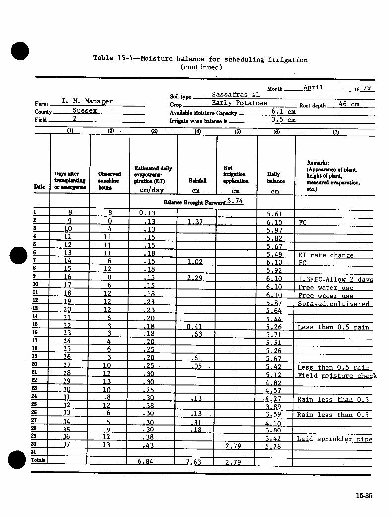
Table 15-4-Moisture balance for scheduling irrigation (continued)
Month April 19 79 Soil tm Sassafras 61
Fm I. M. Manager Early Potatoes 46 cm Caunty Sussex
CmP 6.1 cm
‘Root depth
Availabje Moisture CaPacity Field 2 Irrigate when balance ia 3.5 cm
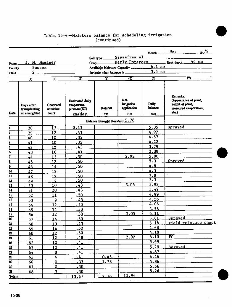
Table 15-4-Moisture balance for scheduling irrigation (continued)
Fm I. M. Manager Caunty -
Field 7
Month %Y 192.L
Roll typ Sassafras sl CmP Earlv%atoes Root depth 46 cm Avahbk Moietutw cepecity 6.1 cm Irrigahwhenbahnoeie 3.5 cm
0
k
68 I 3 I 30 I I I 5.26 I
T0h.h~ 13.67 7-16 I 11.94 I a
15-36

Table 15-4-Moisture balance for scheduling irrigation (continued)
Month June l&E Soil tyIm2 Sassafras sl
FUlll I. M. Manager Cw Early Potatoes Root depth 46 cm
Caunty Sussex AvaiIabje Mo&.ure Capa+ty 6.1 cm Field 2 Irtigak when balmce b 3.5 cm
CEI cm
I I I BaIanceBmugbtF~.~.
1 69 13 0.46 9 70 10 0.3& 8 71 0 0.30 3.23
6 73 8 6 74
75 13 0 36 ! !
7 0:’ 43 I I a 76 8 0. 36 I 0.13 9 I 77 I 8 I 0.G 0.20 10 1 78 10 0.36 11 1 79 j 12 j 0 ’ 38 . . I I .a 1 30 I 3 I 0.25 1 0.25 18 81 12 0.38 14 82 12 0.38 16 83 3 0.2Q 0.25 16 84 0 0.25 1 90 . 17 85 2 0.23 0.36 la 86 10 0.30 19 87 6 0.30 0.84
cm
4.80 4.42
5.31 4.95 4.59 4.23 3.85 3.60 3.22 2.84
FC
ET estimated
Adiusted ET value
Start digging
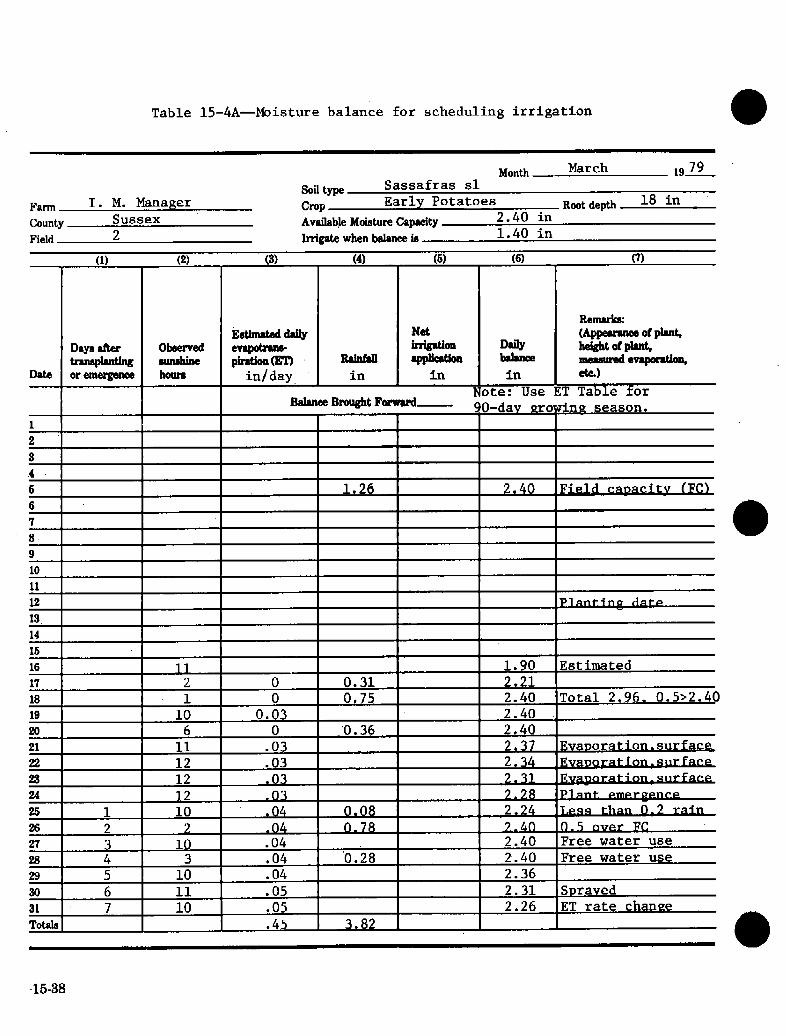
Table 15-4A-Moisture balance for scheduling irrigation
Month March 19 73
Soil typ Sassafras sl Fallll I. M. Manager CmP Early Potatoes Root depth 18 in coullty Sussex Available Moisture Capncity 2.40 in Field 2 1tigat.e when balance b 1.40 in
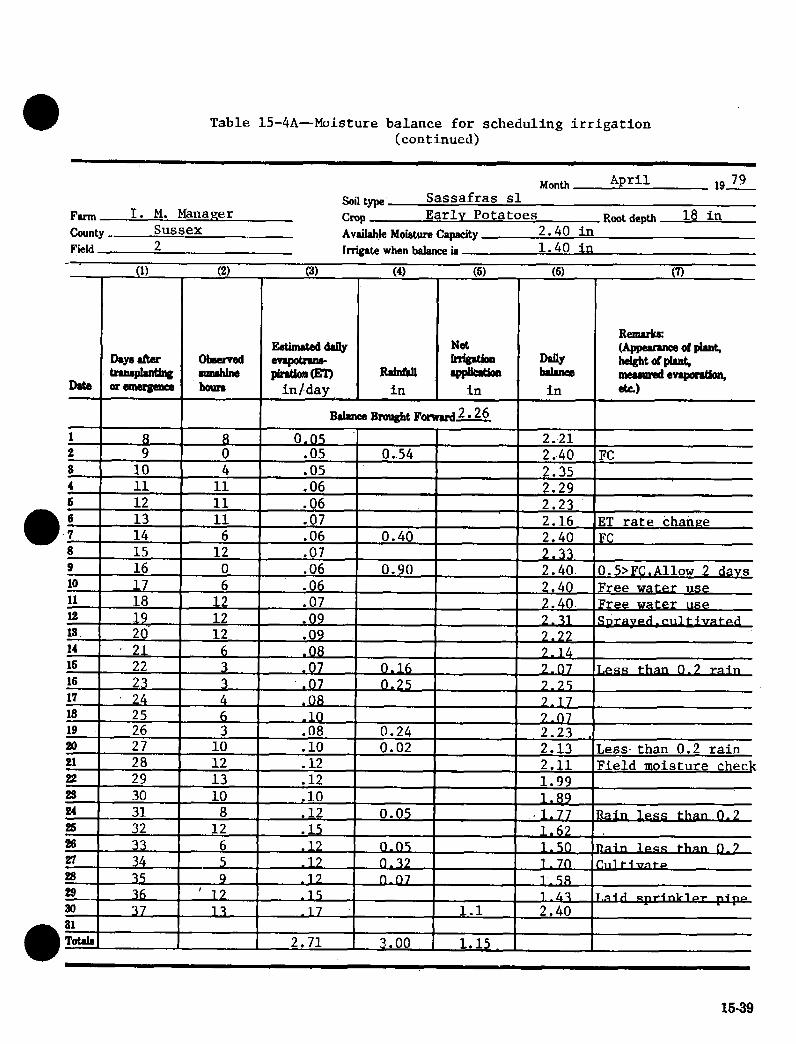
Table 15-4A-Moisture balance for scheduling irrigation (continued)
Month April 192%
%I type Sassafras sl FWltl I. M. Manaper Cw Early Potatoes Root depth 18 in Cmnty Sussex Avnilabje Moisture Capacity 2.40 in Field 2 Imigate when balance in 1.40 in

Table 15-4A-Moisture balance for scheduling irrigation (continued)
Month May 19J.L Sassafras sl
FWnl I. M. Manager Soiltyp CroP Early Potatoes 18 in
Caunty Sussex Availabje Moisture CaPacity 2.40 in Root depth
Field 2 Irrigate when b&me ia 1.40 in

Table 15-4A-Moisture balance for scheduling irrigation (continued)
Month June 19 n Soil typ Sassafras sl
h.t-m~ Cmp Earlv Potatoes Root depth 18 in County SlJ&pX AvailabJeMoi&mCapacity 2.40 in Field 7 Ir+te whenbalanceia 1.40 in
I I I Bdence Bmught Fomdu 1 1 1
1 69 13 0.18 I I
8 I 71 I 0 I -12 1 1.27 I 4 72 15 I
6 74 14 7 75 13 17 8 76 8 14 0.05
1.27 1 1.12 I 1.04 IAdiusted ET value 1s 1 R? I q I I 0.10 I
16 1 RI5 cl 1n 0.75 I 1.69 1.60 1.48
19 R7 6 17 0.23 al RR 17
21 89 z 90
I TOW 1 I I I 7.93 I
1641

Table 16SAample~Estimated values of daily evap tratipiration for obsemed sunshine and crop stage of growth
P?or potatoes during a go-day growing season]
Obsemed weather and hours of sunshine
Cloudy Fair Bright o-3 4-10 11-1s
cmlday in/day cm/day inMay cm/day in/day
O-6 0.10 0.04 lm &g 0.13 0.05 7-12 0.13 0.05 !2a Q&i 0.15 OeO6
13-18 0.15 0.06 Q.l5- 0.18 0.07 19-24 0.18 0.07 !uL QJ& 0.23 0.09 25-30 0.21 0.08 u 0J-Q 0.30 0.12 31-36 0.25 0.10 m m 0.38 0.15 3742 0.28 0.11 Q.35&& 0.43 0.17 4348 0.33 0.13 QQ m 0.50 0.20 49-60 0.33 0.13 Q& QJy 0.50 0.20 61-66 0.33 0.13 Q&-J gJ$ 0.48 0.19 67-72 0.30 0.12 m Q&i& 0.45 0.18 73-78. 0.28 0.11 79.84 0.25 0.10
Qaz 0.43 0.17 QJQ 0.38 0.15
85-90 0.23 0.09 miiii 0.35 0.14
%I cam it is impaeaible to observe weather conditiona over a period of 1 or 2 days, uae the underlined value8 for that period to bring the daily moisture balance up ~JJ date.
3. Should the recordkeeper be away for a day or two, select average values for consumptive use and record them in column 3.
4. Record the amount of rainfall in column 4. Amounts should be recorded to the nearest 0.01 cm (0.01 in).
6. From the preceding day% balance in column 6, subtract the ET use value in column 3. If rainfall exceeds 0.5lcm (0.2 in), column 4, add this value to the daily moisture balance to obtain the new daily balance. If the total exceeds the value for available moisture at field capacity in the root zone, enter in column 6 the available moisture, which has been determined and recorded in the heading of the form. If the total exceeds the available moisture value at field capacity by 1.3 cm (0.6 in) or more, continue the full moisture balance value for 2 succeeding daya as shown in the example (tables 164 and 4A). During this 2day period, the plants will be using the free water in the root zone.
6. Continue the daily accounting process until the balance recorded in column 6 approaches the
1642
value preselected for irrigation to begin. The daily balance shows the amount of remaining available moisture and indicates the amount of irrigation to be scheduled. The net irrigstion to be applied is the difference between the current daily balance prior to the start of irrigation and available moisture- holding capacity plus the estimated evapotransptia- tion for that day. The gross application is the re- quired net application divided by the expected ap- plication efficiency (expressed as a decimal). Add the net irrigation amount to the daily moisture balance to obtain the new daily balance. If some ef- fective rainfall occurs during the irrigation, add this to the Wigation applied. As stated in item 5, irrigation plus rainfall should bring the soil to field capacity, but the balance cannot exceed the moisture-holding capacity of the soil.
Follow the= six steps at the end of each day dur- ing the growing season until the crop hm reached the desired maturity.
Aauetment Facbn
If the daily moisture balance is allowed to drop below 60 percent of the total available moisture value, plants have increuing d.ifiIculty obtaining the moisture they need for vigorous growth. In such cases, daily evapotranspiration will be reduced.
If the crop was not irrigated when the daily moisture balance reached the 60-percent level, ET values from table 15-5 must be reduced. The actual reduction in ET rates varies with the kind of crop. However, the following factors can be used as a guide for estimating probable daily ET rates. For lowered moisture levels, multiply the value ob- tained from table 15-5 by the applicable factor for the existing moisture level.
Moisture level percent Factor 40-50 0.8 30-40 0.6 20.30 0.2
Irrigation Rocedure
If several days are required to irrigate the crop, the application for each succeeding day should be increased by the day’s consumptive use. If more than 3 days are required to complete the irrigation, the following method may be used to adjust the ap plication requirements:

Direct Gas Pressure Method for Scheduling Irrigation
l 1. Divide the number of days required to com- plete the irrigation into 2- or 3lday intervals.
2. Add 0.75 cm (0.3 in) or 1.3 cm (O-5 in), respectively, to the net application amount used for the previous interval. Variations of this procedure may be used to fit in- dividual situations.
Some operators regard keeping a daily moisture accounting record as burdensome. G. W. Eley and He M. Kautz developed an equally or more accurate method that requires only occasional soil moisture checks. The irrigator can refer to the Soil Characteristics Sheet (table 15-6) for the particular area of the field to obtain the percentages of available moisture remaining and the centimeters (inches) of water needed in the effective root zone depth of the crop.
The equipment consists of a soil volume sampler, a sample drier, and a supply of Field Moisture Check Forms and Soil Characteristics Sheets. The Eley volumeter and a carbide moisture tester are used in this procedure. A tube sampler with an ex- tension handle is convenient for sampling soils for moisture content after bulk densities have been determined.
This simplified method of irrigation water management eliminates daily recordkeeping and the need for estimating the effect of climatic factors and the stage of crop growth on daily consumptive use. It requires no accounting for soil moisture changes caused by rainfall or irrigation.
Once the Soil Characteristics Sheets have been developed for specific areas in the field, the ir- rigator needs to make carbide moisture tests of samples from appropriate depths in the field and refer the gage readings to the Soil Characteristics Sheets. The net centimeters (inches) of water to be applied to an area are the sum of the values for the soil layers sampled in the effective root zone depth.
lt is necessary to have a Soil Characteristics Sheet for each typical soil or control area in the field. One Soil Characteristics Sheet will apply to all crops in the same area by using the appropriate effective root zone depths.
The irrigator should be given technical assistance to develop at least the first Soil Characteristics Sheet. In the interest of providing training and reducing the number of samples to be taken, it would be desirable for the technician to assist in developing the Soil Characteristics Sheets and to include the root zone depths for all crops to be grown in a particular field or fields.
Sample Froblcm
The following example outlines the procedure for preparing the Soil Characteristics Sheet. (See table 15-6.)
1543

Table 15-6.
Soil Characteristics Sheet for Irrigation Water Management Field: 3 Crop: potatoes
Farm: Sample Location: Upper end
T Available Moisture Level’
Field Capacity2
18.9%
o- to 8-h)
Wilting Point’ 3.8%
(Applies ta all Wml
(percent)
W Weight
Moisture (Percent)
Speedy Tester Gage
Readin&
100 (F.C.) 18.9 16.4
90 17.4 16.3
80 16.9 14.2
707 14.4 13.1
607 12.9 11.9 507 11.3 10.6
40 9.8 9.3
30 8.3 7.9 20 6.8 6.5
10 5.3 5.2
0 (W.P.) 3.3 3.8
0 to 2&m Soil Layer
Rulk Density4
1.66 g/cma
Net Water
to Apply6 (cm) (in.)
0.48 0.19
0.96 0.38
1.46 0.57 1.93 0.76
2.41 0.95 2.90 1.14
3.38 1.33
3.86 1.62
4.34 1.71
4.s 1.90
l- I
2& to 38-cm Soil Layer
Field Capacity
17.1%
3- to 16in. Wilting
Point 3.4%
Bulk ‘Field Density Capacity
1.50 g/cm3 18.2%
5- to 13-m Wilting
Point 4.6%
W Speedy Net DW Swdy Weight Tester Water Weight Tester
Moisture Gage to APPLY Moisture Gage (Percent) Reading (cm) (in.) (percent) Reading
17.1 15.1
15.7 14.1
14.4 13.1 13.ci ’ 12.0 11.6 10.8 10.3 9.7
8.9 8.5
7.5 7.2
6.1 6.9
4.8 4.8
3.4 3.4
0.36 0.14
0.71 0.28
0.67 0.42
I.42 0.56
I.78 0.70
2.13 0.84
2.49 0.98
2.34 I.12
3.20 1.26
3.56 1.40
18.2 15.9
16.8 14.9
15.5 13.9
14.1 12.8 12.8 11.8 11.4 10.7 10.0 9.5
3.7 8,3
7.3 7.0
6.0 5.3
4.6 4.6
T I
33- to 45-cm Soil Layer
Bulk Density
1.45 g/cm’
Net Water
to APPLY (cm) (in.)
0.15 0.06 0.30 0.12
0.46 0.18
0.61 0.24
0.76 0.30
0.91 0.36 1.07 0.42
1.22 0.48
1.37 0.54
1.52 0.60
1 The ratio of the centimeters (inches) of remaining available moisture to the field capacity in a specific soil layer, expressed as a percent. (One hundred (100) percent equals Field Capacity; zero (0) percent equals Permanent Wilting Point.)
2 A field measurement of the amount of water retained in a well-drained soil, 1 to 4 days after a thorough wetting by rainfall or irrigation, expressed as a percent of the dry weight of the soil.
’ The moisture content, expressed as a percent of the dry weight of the soil, at which plants can no longer extract moisture.
’ The ratio of dry weight of the sample in grams to.its volume in cubic centimeters. s The moisture content of a specific soil sample, expressed as a percent of the wet weight of the soil. * Net centimeters (inches) of water to bring the soil layer to field capacity. When different soil layers are utilized by a crop, the total net
application is the sum of the net amounts required for each soil layer. ’ Desirable time to start irrigation, depending on the crop and number of days required to irrigate the crop.
Given: Soil-sassafras sandy loam,
O-20 cm (O-8 in) Dark-brown sandy loam; weak, fine granular. structure; very friable.
20-38 cm (8-15 in) Yellowish-brown sandy loam; structureless to weak, medium subangular blocky structure; friable.
38-60 cm (1524 in) Yellowish-brown sandy loam; weak, fine to medium subangular blocky structure; some very fine roots; some wormholes, and wormcasts.
Irrigated crops: peas, peppers, potatoes, snap- beans Effective root depth: 30 to 45 cm (12 to 18 in)
0 -
a 15-44

Moisture Percentage at Field Capacity
Determine the percentage of moisture at field capacity in each soil layer, using a carbide moisture tester and Eley volumeter.
1. Dig a hole slightly beyond the effective root depths to be considered.
2. Record in the heading of the Soil Character- istics Sheet the range in depth of the diEerent aoil layers and include effective root zone depths of crops to be irrigated. Use additional sheeta if necessary.
3. Take test samples of the different textural layers as shown in tigure 156.
4. Weigh a 26-g (0.92-0s) sample from the test sample taken from each layer with the volumeter. Record the volume of soil required to equal 26 g (0.92 021. Determine the moisture percentage in each weighed sample by using the carbide moisture tester. The gage reading is the moisture percentage based on wet weight of the sample.
5. Record the gage reading for each soil layer on the line of the Soil Characteristics Sheet op posite 100 (F-C.). Convert these values to percent- age of moisture based on dry weight of the sample by using the carbide moisture tester conversion chart (exhibit 15-6).
Flgure 15-6
Sampling of Textural Layers
15
30
cm
cm
cm
cm
cm
For example: Moisture Percent
tester moisture,
(cm) Soil layer
(in) i3w
reading dry w&g& of sample
O-20 O-8 16.4 18.9 20-38 8-15 15.1 17.1 38-60 1524 15.9 18.2
6. Record the dry weight moisture percentage for each soil layer on the line of the Soil Character- istics Sheet, table 156, opposite 100 (PC.).
Bulk Density Measurement
Compute the bulk density of the soil in each layer, using the formula:
Bulk Density = Weight of Sample
Volume of Sample (1 + Percent Moisture, Dry Weight) 100
Where: Weight of samples equals 26 g (0.92 oz). Volumes of samples equals 14.0, 14.8, and 15.2 cma (0.85, 0.90, and 0.93 ix?), respectively. (Obtained while getting moisture percentage at field capa- city.) Percent moisture, dry weight, equals 18.9, 17.1, and 18.2, respetively.
O- to 2O-cm CO- to 8+inI layer:
Bulk Density = ~14~o~~+ UIQ) = l4.0?189) =
1.56 glcrn
20- to 38-cm (8- to 15-m) layer:
1.50 g/cm’

38- to 60-cm (15- to 24~in) layer:
1.45 g/ems
Record these values for the different layers in the spaces for bulk density in the heading of the Soil Characteristics Sheet.
Moisture Percentage at Wilting Point
From laboratory or other dependable data, obtain the moisture percentage at 15 atmospheres of soil moisture tension for the type of soil to be irrigated. If this information is not available, use the follow- ing fractions to estimate the moisture percentage at wilting point for each soil layer (not applicable to saline soils).
1. For loamy fme sand, use one-sixth of the field capacity percentage.
2: For very fme sandy loam, use one-fifth of the field capacity percentage.
3* For fine sandy loam, use one-fourth of the field capacity percentage.
4. For sand, sandy loam, loamy sand, loam, and silt loam, use one-third of the field capacity percentage.
6. For silty clay and clay, use one-half of the field capacity percentage. Record these values in the spaces for wilting point in the heading of the Soil Characteristics Sheet.
Centimeters (Inches) of Available Moisture
Compute the centimeters (inches) of available moisture for each soil layer to the effective root depth selected. Use the values recorded in the up- per part of the Soil Characteristics Sheet for each soil layer.
Available Moisture=
Field Capacity - Wilting Percentage x Bulk Density x Depth of Soil Layer
100 x 1
O- to 2O-cm layer:
Available Moisture = (18.9 - 3.8~1.66)@0)
100 x 1 4.71 cm, we 4-70 cm
0- to &in layer:
Available MoiFture = (16.9 - 3.3X1.66)(8)
= 1.89 in, use L90 in 100x 1
20- to 38~cm layer:
Available- Moisture - (17.1 - 3.4Xl.EoXlsL 3,6g cm use 3 7. cm 100 x I
8- to 15in layer:
Available Moisture = (17” - 3’4X1’6oX7)= 1.44 in use ~.40 in 100x1
38- to 45-cm layer?
Available Moisture = (18.2 - 4.6X1*45X7)= 1.cJ.a cm u5e 140 cm loo x 1
15 to 18- in layer:
Available Moisture = “‘-’ ~~*~~43x3’= 0.59 in, use 0.60 in
Total Available Moisture to 45-cm (18-in) root depth = 9.8 cm-(3.9 in)
Net Moisture Requirement at Each Moisture level
Beginning with the “available moisture level” of zero at the bottom of the “Equivalent Moisture Table” (exhibits 15-7 and 7A), follow horizontally until a number is found that is equal to the cen- timeters (inches) of available muisture at field capacity for the soil layer. Copy this column of figures onto the Soil Characteristics Sheet in the column headed “Net Water to Apply.” Repeat for each soil layer.
Determining Adjustment Percentages
Calculate for each soil layer the adjustment percentage needed to relate percentage moisture
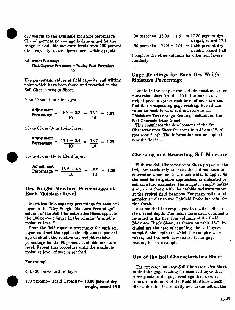
dry weight to the available moisture percentage. The adjustment percentage is determined for the range of available moisture levels from 100 percent (field capacity) to zero (permanent wilting point).
Adjustment Percentage = Field Capaciw Percentage - Wking Point P-II-
10
Use percentage values at field capacity and wilting point which have been found and recorded on the Soil Characteristics Sheet.
0- to 20-cm (O- to $-in) layer:
Adjustment 18.9 - 3.0 = 16.1 = 1.51 Percentage = 1.
Y-ii-
20+ to 38-cm (8- to 15-in) layer:
Adjustment 17.1 - 3.4 = 13.7 = 1.37 Percentage = 1. TiT
38- to 46-cm (15- to 18-in) layer:
Adjustment Percentage = 18.2 - 4.6 = 13.6 = 1.33 1. Tii
Dry Weight Moisture Percentages at Each Moistutie level
Insert the tield capacity percentage for each soil layer in the “Dry Weight Moisture Percentage” column of the Soil Characteristics Sheet opposite the loo-percent figure in the column “available moisture level.”
From the tield capacity percentage for each soil layer, subtract the applicable adjustment percent- age to obtain the relative dry weight moisture percentage for the go-percent available moisture level. Repeat this procedure until the available moisture level of zero is reached.
For example:
O- to 20.cm CO- to 8-m) layer:
l 100 percent= Field Capacity= 18.90 percent dry weight, rec& 18.9
90 percent= 18.90 - Ml = 17.39 percent dry weight, record 17.4
80 percent= 17.39 - 1.51 = 15.86 percent dry weight, record 16.9
Complete the other columns for other soil layers similarly.
Gage Readings for Each Dry Weight Moisture Percentage
Locate in the body of the carbide moisture tester conversion chart (exhibit 15-6) the correct dry weight percentage for each level of moisture and find its corresponding gage reading. Record this value for each level of soil moisture in the “Moisture Tester Gage Reading” column on the Soil Characteristics Sheet.
This completes the development of the Soil Characteristics Sheet for crops to a 45cm (18-m) root zone depth, The information can be applied now for field use.
Checking and Recording Soil Moisture
With the Soil Characteristics Sheet prepared, the irrigator needs only to check the soil moisture to determine when and how much water to apply. As the need for irrigation approaches, as indicated by soil moisture estimatis, the irrigator simply makes a moisture check with the carbide moisture tester at the typical field locations. For many soils, a tube sampler similsr to the Oakfield Probe is useful for this check.
Assume that the crop is potatoes with a 45~cm (18-in) root depth, The field information obtained is recorded in the first four columns of the Field Moisture Check Sheet, as shown on table 15-7. In- cluded are the date of sampling, the soil layers sampled, the depths at which the samples were taken, and the carbide moisture tester gage reading for each sample.
Use of the Sd Characteristics Sheet
The irrigator uses.the Soil Characteristics Sheet ,to find the gage reading for each soil layer that corresponds to the gage readings that were re- corded in column 4 of the Field Moisture Check Sheet. Reading horizontally and to the left on the
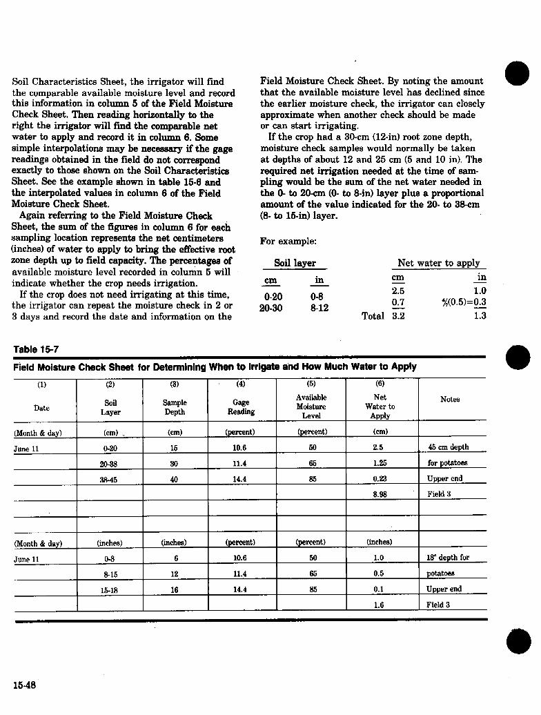
Soil Characteristics Sheet, the irrigator will find the comparable available moisture level and record this information in column 5 of the Field Moisture Check Sheet. Then reading horizontally SKI the right the irrigator will find the comparable net water to apply and record it in column 6. Some simple interpolations may be necessary if the gage readings obtained in the field do not correspond exactly to those shown on the Soil Characteristics Sheet. See the example shown in table X-6 and the interpolated values in column 6 of the Field Moisture Check Sheet.
Again referring to the Field Moisture Check Sheet, the sum of the figures in column 6 for each sampling location represents the net centimeters (inches) of water te apply to bring the effective root zone depth up te field capacity. The percentages of available moisture level recorded in column 5 will indicate whether the crop needs irrigation,
If the crop does not need irrigating at this time, the irrigator can repeat the moisture check in 2 or 3 days and record the date and information on the
Table 15-7
Field Moisture Check Sheet. By noting the amount that the available moisture level has declined since the earlier moisture check, the irrigator can closely approximate when another check should be made or can start irrigating.
If the crop had a 30-cm (124n) root zone depth, moisture check samples would normally be taken at depths of about 12 and 25 cm (5 and 10 in). The required net irrigation needed at the time of sam- pling would be the sum of the net water needed in the 0- to 20~1n (O- to El-in) layer plus a proportional amount of the value indicated for the 20- to 38-cm (8- to 154n) layer.
For example:
Soil layer Net water to apply
cm
O-20 20-30
in
O-8 a-12
cm 2.5 0.7
Total 3.2
in ii
X(0.5)=0.3 iz
Field Moisture Check Sheet for DetermInIng When to lrrlgate ahd How Much Water to Apply
(11 (21 (31 (4) I (5) I (61
Date soil
Layer Sample Depth
@UP Fteadimg
Available Moisture
Level
Net Water to
APPLY
16-18 16 14.4 86 0.1
1.6
Notes
46 cm depth
for potatoes
Upper end
Field 3
13” depth for
potatoes
Upper end
Field 3
1648

EXHIBITS

Exhibit 15-l
lrrlgation Ditch Sections with Required Lateral Beds
Water surfaces
Lateral Bed Before Ditch is Pulled
F n=
s = 0.00: S= 0.062 s = 0.003
n = 0.03 I n = n= 0.03 n = 0.04
Q --I- I’ Q
n=
V
7 Drtcl
No. b -
2L 0.5
W R
-r -F
1.06 8.5
A R V I I V d F
ft ft
1.0 0.5
1.0 0.5
1.0 0.5
1.0 0.5
1.2 0.7
1.2 0.7
1.2 0.7
1.33 0.7
1.33 0.7
1.5 1.0
1.5 LO
1.75 1.1
1.75 1.1
, 1.75 1.1
,2.0 1.3
,2.0 1.3
fWS ft% ftlS ftls ftvs
1.03 2.1
1.10 2.8
1.17 3.5
1.21 4.2
1.22 4.1
1.28 5.1
1.33 6.1
1.36 6.3
L41 7.5
1.50 9.6
1.59 12.5
1.64 13.3
1.73 17.0
1.80 ., 20.9
1.86 22.3
1.93 27.0
612 15 d 2.0
2.5
1.37
1.47
1.50
2.7 x 1.79
#1.91
1.97
1.99
1212
1812
1.0 - 1.5
1.56
2.06
10.0
11.5
3.7
4.7
5.6
5.5
6.3
8.1
8.4
10.0
12.8
16.3
17.7
22.7
27 a L 29.6
36.0
2412 2.0 2.50 13.0
1.25 11.3
1.56 12.3
3.50 0.62 0.81
#
2.8 0.60
3.36 0.63 0.81
* 2.7 0.61
3.96 0.68 0.86 3.4 0.64
2.1
2.0
2.5
3.0
2.9
3.6
4.3
4.5
5.3
6.8 -Y-- 8.8
9.3
12.0
14.7
15.7
19.0
1.61
1.63
1.71
1.78
1.81
1.33
2.00
2,13
2.19
2.30
2.40
2.47
2.57
1.13 4.0 0.86
1.15 ‘3.9 0.87
1.21 4.8 0.91
1.25 5.7 0.94
1.28 6.0 0.96
1.33 7.1 0.99
1.42 9.1 1.06
1.50 11.8 .1.12
1.55 12.6 1.15
1.63 16.1 1.22
1.70 19.7 1.27
1.75 21.0 1.31
1214
la14
1.0 - 1.5 2.09
2.18
2.22
2.30
2.45
2.60
2.67
2.a2
2.94
3.03
3 15 L
8.3 1.57 6.2
9.9 1.63 7.4
10.4 1.06 7.7
12.3 1.72 9.2
15.6 1.83 11.7
20.5 1.95 15.4
21.6 2.00 16.2
27.8 2.11 20.8
34.1 2.21 25.6
36.4 2.27 27.2
44.1 2.36 33.0
2.0 - 1.5 - 2.0
4.56 0.72 0.89
#
4.1 0.67
4.65 0.74 0.90
* 4.2 0.68
5.31 0.78 0.94 4.9 0.71
3.1
3.2
3.3
4.8
6.3
6.6
2414
1816
2416
13.8
13.6
14.6
2.0 - 3.0 - 2.0
15.5
17.5
17.4
6.33 0.86 1.00
#
6.4 0.75
7.3a 0.94 1.06
* 8.4 0.80
8.10 0.98 1.09 8.8 0.82
2418
3618
2421
3.0 - s
3.0 - g
19.9
21.9
21.3
22.8
11.3 0.86
13.9 0.90 3 14.9 0.93
17.9 0.96
8.5
10.4
11.2
3621
4321
3624
4324 13.4 I.32 1 25.5 1 1.36
A = Cross-sectional area in square feet. R = Hydraulic radius in feet. n = Coefficient of roughness.
Use n = 0.03 for, bare ground. Use n = 0.04 for grassed ditch bottom.
s = Slope in feet per foot V = Velocity in feet per second Q = Capacity of ditch in cubic feet per second.
15-50

Exhibik 15.2-Relief classes for surface-irrigat4 land.

Discharge of Aluminum Siphon Tubes at Various Heads
2 5 (L= Length of tube)
10 20 50 loo Discharge (gallons per minute)
200 500 800
Exhlblt 15-4
MultIpIe Outlet Factor for Gated Pip
Number of Multiple Outlet Outlets FaCtJW
5 o-44
10 0.39
15 0.37
20 0.86
SO 035
50 0.34
100 0.34
m 0.33
16-62

Tap: 0 to 33% d slightly crueted. Will
“ball” with pressure but breaks ~~~~r~~ eaGly. &V&Y 34 to 66% available moisture-forms a ball under pies *a, Somewhat
ti3 pressure. iI1 “ribbon out” be” tweexi thumb ottoYn.” 67 to 0% tivailablo moi~~~“ball5” readilv. “Ribbons out” e&Iv.
) tedium Texture. Top; 0 to 33% available to hold together with hand pressure but
crumbles easily. Center: 34 to 66% available moisture-forms a ball unde ressure~ Somewhat plastic. “Slicks” slightly with pressure. ottam: 67 to 100% available moisture-forms a ball easily. Is very pliable. “Slicks” readily.
15-53
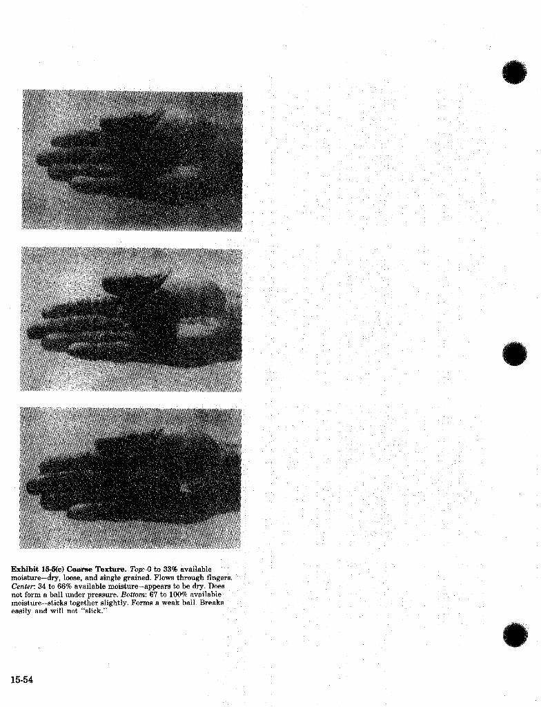
Exhibit l&%(c) Coarse Texture. !Z’OJX~ to 33% available moistur e-dry, loose, and single grained. Flows through fingers. Center: 34 to 66% available moisture-appears to be dry. Does not form a ball under pressure. Bottom: 67 to 100% available moisture-sticks together slightly. Forms a weak hall. easily and will not “slick.”
15-54

CarbIde Molsture Tester ConversIon Chart WP Reading’
2
3
4 5
-r 0.2
2.2 3.2
4.2
5.3
6
7 8
9 10
6.4
7.6 8.6
9.7
10.8
11
12 13
14
15
12.0
13.3
14.6
16.9
17.3
16
. . 17 .-. 18
0 0.1
2.0 2.1 3.0 3.1
4.0 4.1
5.1 6.2
6.2 6.3
7.3 7.4 a.4 8.5
9.6 9.6
10.6 10.7
11.8 11.9
13.0 13.1 14.3 14.4
16.6 a.7
17.0 17.1
18.3 18.4 19.7 19.8
21.1 21.3 22.6 22.8
24.1 24.3
2b.6 26.8 27.1 27.3
28.6 28.a 30.2 30.4
31.7 31.9
33.3 33.6
34.9 35.1 36.5 36.7
38.1 39.3 39.8 40.0
41.6 41.7
43.2 43.4
44.8 45.0
’ Carbide moisture tester-3-minute readings.
19
20
21
22
23 24
25
26 27 28
29 30
18.6
20.0
21.4 22.9
24.4
26.9 27.4
28.9 30.6
32.0
33.6
a.2 36.8
39.4 40.1
31 32
33
41.8
43.5 4s.i
2.3 3.3
4.3
6.4
6.6
7.6 8.7
9.8
11.0
12.2
13.4 14.7
16.0
17.4
18-7
20.i
21.6 23.1
24.6
26.1
27.6
29.1 30.7
32.2
33.8 36.4 37.0
39.6 40.3
42.0 43.7
46.3
2.4 3.4
4.4
6.5
6.6
7.7 8.8
9.9
11.1
12.3
13.5 14.8
16.2
17.5
18.9
20.3.
21.7 23.2
24.7
26-2
27.7
29.2 30.8
32.3
33.9 35.5 37.1
33.a 40.6
42.2 43.8
46.5
- e @scent1
0.5
2.6 3.5
4.6
6.7
6.8
7.9 9.0
10.1
11.2
12.4
13.7 16.0
16.3
17.7
19.0
20.4
21.9 23.4
24.9
z.4 27.9
29-4 31.0
32.5
34.1 36.7 37.3
39.0 40.7
42.4 A.0
45.7
-
0.6
2.6 8.6
4.6
6.8
6.9
8.0 9.1
10.2
11.3
12.5
13.8 15.1
16.4
17.8
19.1
20.6
22.0 !23.5
25.0
26.6
28.0
29.6 31.1
32.7
34.3 35.9 37.5
39.1
40.8
42.5 44.2
45.8
0.7
2.7 3.7
4.7
6.9
7.0
8.1 9.2
10.3
11.4
12.6
13.9 16.2
16.6
17.9
19.3
20.7
22.2 23.7
26.2
26.7
28.2
29.7 31.3
32.8
34.4 36.0 37.6
39.3
41.0
42.7
44.3 46.0
0.8
2.8 3.8
4.8
6.0
7.1
a.2 9.3
10.4
11.6
12.8
14.0 16.3
16.7
18.0
19.4
20.8
22.3 23.8
25.3
26.8
28.3
29.9 31.4
33.0
34.6 36.2 37.8
39.6 41.2
44.9 44.6
46.2
0.9
2.9
3.9
4.9
6.1
7.2 8.3
9.4
10.5
11.7
12.9 14.2
15.5
16.9
18.2
19.6
21.0
22.5 24.0
26.6
27-O
28.5
30.0 31.6
33.1
34.7 36.3 37.9
39.6 41.3
43.0 44.6
46.3
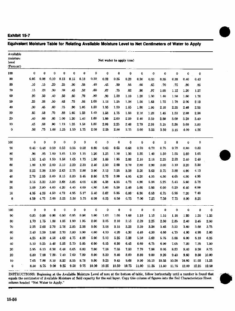
Exhlblt 15-7
Equivalent Molsture Table for Relating Avallable Molsture Level to Net Centimeters of Water to Apply
Available moisture level Net water to apply (cm)
(Percent)
100 0 0 0 0 0 0 0 0 0 0 0 0 0 0 0 0 90 0.05 0.08 0.10 0.13 0.16 0.18 0.20, 0.23 0.25 0.28 0.30 0.33 0.35 0.38 0.40 0.43 80 .lO .lS .20 .2s .30 .35 .40 .4S 30 .ss .60 A5 .70 .75 30 .8S 70 .15 2.3 .30 38 .45 .52 A0 .67 .7s .82 30 .97 1.06 1.12 1.20 1.27 60 .20 .30 .40 .50 .60 .70 30 .90 1.00 1.10 1.20 1.30 1.40 1.50 1.60 1.70 so 25 .38 .50 A3 .75 .88 1.00 1.13 1% 1.38 l*SO 1.63 1.75 1.78 2.00 2.13 40 .30 .45 A0 .75 .90 1.05 1.20 1.35 1.60 1.65 1.80 1.95 2.10 2.25 2.40 2.55 30 .3s .s3 .70 38 1.06 1.23 1.40 1.53 1.75 1.83 2.10 1.23 1.46 1.53 2.80 2.98 20 .40 .60 30 1.00 1.20 1.40 1.60 1.80 2.00 2.20 2.40 2.60 2.80 3.66 3.20 3.40 10 .45 38 20 1.13 1.35 1.53 1.80 2.03 2.26 2.42 2.10 2.93 3.15 3.38 3.60 3.33 0 .50 .75 1.00 1.25 1.50 1.76 2.00 2.2s 2SO 2.75 3.00 3.25 3.50 3.15 4.00 4.26
100 0 0 0 0 0 0 0 0 0 0 0 0 0 0 0 0
90 0.45 0.48 0.60 O.S3 0.65 0.58 0.60 0.63 0.66 0.68 0.70 0.73 0.76 0.78 0.80 0.83
80 .90 .95 1.00 1.05 1.10 1.15 1.20 1.26 1.30 1.30 1.35 1.40 1.50 l.SS 1.60 1.65 70 1.36 1.43 1.50 158 1.65 1.73 1.80 1.38 1.95 2..03 2.10 2.18 2.25 2.33 2.40 2.48
60 1.80 1.90 2.00 2.10 2.20 2.30 2.40 2.50 2.60 2.70 2.30 2.90 3.00 3.10 3.20 3.30
50 2.25 2.38 2.SO 2.63 2.76 2.83 3.00 3.13 3.26 3.38 350 3.63 3.76 3.33 4.09 4.13
40 2.70 2.85 3.00 3.15 3.30 3.45 3.60 3.7S 3.90 4.06 4.20 4.35 4.50 4.65 4.80 4.95 30 3.15 3.33 3.SO 3.63 3.85 4.03 4.20 4.33 4.55 4.73 4.96 6.08 5.25 5.43 5.60 5.78
20 3.60 3.80 4.00 4.20 4.40 4.60 4.80 5.00 5.20 5.40 5.60 5.80 6.00 6.20 6.40 6X0
10 4.05 4.23 4.SO 4.73 4.95 5.17 5.40 5.62 6.85 6.08 6.30 6.63 6.76 6.98 7.20 7.43 0 4.50 4.75 5.00 5.25 5.60 6.76 6.00 6.25 650 6.75 7.00 7.25 7.50 7.7s 8.00 8.2S
100 0 0 0 0 0 0 0 0 0 0 0 0 0 0 0 0 0 90 0.86 0.88 0.90 0.93 0.95 0.98 1.00 1.03 1.05 1.08 1.10 1.13 1.15 1.18 1.20 1.25 1.2S
80 1.70 1.75 1.80 l&i 1.90 1.95 2.00 2.05 2.10 2.15 2.20 2.25’ 2.30 2.36 2.40 245 250 70 2.55 2.63 2.70 2.78 2.85 2.93 3.00 3.03 3.15 3.22 3.30 3.38 3.45 3.53 3.60 3.68 3.7s
60 3.40 3.50 330 3.70 3.30 3.90 4.00 4.10 4.20 4.30 4.40 4.So 4.60 4.70 4.80 4.90 s.Ml so 4.26 4.38 4.60 4.63 4.75 4.38 5.00 5.13 5.25 6.38 6.60 5.63 5.75 5.38 6.00 6.13 6.25 40 5.10 6.26 6.40 5.55 5.70 5.35 6.00 6.15 6.30 6.45 6.66 6.76 6.90 7.05 7.20 7.35 7.50
30 5.95 6.13 6.30 6.48 6.65 6.33 7.00 7.18 7.35 753 7.70 7.38 8.05 8.23 8.40 8.53 8.75
20 6.80 7.00 7.20> 7.40 7.60 7.80 8.00 8.20 8.40 8.60 8.30 9.00 9.20 9.40 9.60 9.80 1o.m 10 7.65 7.88 8.10 8.33 8.55 8.78 9.00 9.23 9.45 9.63 9.90 10.13 10.35 10.53 .10.80 11.03 11.25 0 8.50 8.76 9.00 9.26 9.50 9.75 10.00 10.25 10.56 10.75 11.00 11% 1150 11.75 12.00 12.25 12.50
INSTRUCTIONti Beginning at the Avsilable Moisture Level of zero at the bottom of table, follow horizontaiIy until a number is found that equals the centimeter of Available Moisture at fieId capacity for the soil Iayer. Copy this column of figures into the Soil Characteristics Sheet column hesded “Net Water to Apply.”
16-56

Exhibit 157A
Equivalent Moisture Table for Relating Avaiisbie Moisture Level to Net inches of Water to Apply
Available moisture level (Percent)
Net water to apply (in)
100 0 0 0 0 0 0 0 0 0 0 0 0 0 0 0 0 90 0.02 0.03 0.04 0.05 0.06 0.07 0.08 0.09 0.10 0.11 0.12 0.13 0.14 0.15 0.16 0.17 a@ A4 A6 .08 .lO .12 .14 .16 .18 .20 ‘22 .24 .26 .28 .30 .32 .34 70 46 .09 .12 .lS .18 .21 .24 .27 .30 33 .36 .39 .42 -45 .48 -51 60 .oa .12 .16 .20 .24 .28 .32 .36 .40 .44 .48 .52 .56 .60 .64 A8 so .lO .15 .20 .25 .30 .35 .40 .45 .so .ss .60 .65 .I0 .I6 .a0 .85 40 .12 .18 .24 .30 .36 a42 .48 54 .60 .66 -72 .I8 .a4 .90 36 1.02 30 .14 .21 28 .35 .42 .49 36 A3 -70 .I7 .a4 .91 .98 1.05 1.12 1.19 243 .16 24 .32 .40 .48 .56 A.4 .I2 .&II 28 .96 1.04 l-12 1.20 1.28 1.36 10 .18 .27 .30 .45 34 A3 .72 .81 xl .99 1.08 1.17 1.26 1.35 1.44 1.53 0 .20 .30 .40 .so A0 .I0 .a0 .90 1.00 1.10 1.20 1.30 1.40 1.60 1.60 1.70
100 0 0' 0 0 0 0 0 0 0 0 0 0'0 0 0 0 90 0.18 0.19 0.20 0.21 0.22 0.23 0.24 0.25 0.26 0.27 0.28 0.29 0.30 0.31 0.32 0.38 80 .36 38 .40 .42 .44 .46 A8 .50 .52 .M 56 .58 .60 .62 .64 36 70 34 37 A0 A3 .66 .69 .72 .I5 .I8 .81 .84 .87 30 .93 26 39 60 .72 .76 A0 2.4 38 .92 .96 1.00 1.04 1.08 1.12 1.16 1.20 1.24 1.28 1.32 SO 30 .95 1.00 1.05 1.10 1.16 1.20 1.25 1.30 1.35 1.40 1.45 1.50 1.55 1.60 1.65 40 1.08 1.14 1.20 1.26 1.32 1.38 1.44 1.50 1.56 1.62 1.68 1.74 1.80 1.86 1.92 1.98
30 1.26 1.33 1.40 1.47 1.54 1.61 1.68 1.75 1.82 1.89 1.96 2.03 2.10 2.17 2.24 2.31 20 1.44 1.52 1.60 1.63 1.76 1.84 1.92 2.00 2.08 2.16 2.24 2.32 2.40 2.48 2.56 2.64 10 1.62 1.71 1.80 1.89 1.98 2.07 2.16 2.25 2.34 2.43 2.52 2.61 2.70 2.79 2.83 2.97 0 1.80 1.90 2.00 2.10 2.20 2.30 2.40 2.50 2.60 2.70 2.80 2.90 3.00 3.11~ 3.20 3.30
100 0 0 0 0 .o 0 0 0 0 0 0 0 0 0 0 II I3 90 0.34 0.35 0.36 0.37 0.38 0.39 0.40 0.41 0.42 0.43 0.44 0.45 0.46 0.47 0.48 0.49 0.60 80 .68 .70 .72 .74 .76 .78 .a0 .82 34 26 28 .90 .92 .9i 36 .98 1.00 70 1.02 1.05 1.08 1.11 1.14 1.17 1.20 1.23 1.26 1.29 1.32 1.35 1.38 1.41 1.44 1.47 1.50 60 1.36 1.40 1.44 1.48 1.52 1.56 1.60 1.64 1.68 1.72 1.76 1.80 1.84 1.88 1.92 1.96 2.00 so 1.70 1.75 1.80 1.85 1.90 1.95 3.00 2.05 2.10 2.15 2.20 2.25 2.30 2.35 2.40 2.45 ..2.50 40 2.04 2.10 2.16 2.22 2.28 2.34 2.40 2.46 2.52 2.58 2.64 2.70 2.76 2.82 2.83 2.94 3.00 30 2.38 2.45 2.52 2.59 2.66 2.73 2.80 2.87 2.94 3.01 3.08 3.15 3.22 3.29 3.36 3.43 3.50 243 2.72 2.80 2.88 2.96 3.04 3.12 3.20 3.28 3.36 3.44 3.52 3.60 3.68 3.76 3.84 3.92 4.m 10 3.00 3.15 3.24 3.33 3.42 3.61 3.60 3.69 3.78 3.87 3.M 4.05 4.14 4.23 4.32 4.41 4.50 0 3.40 3.50 3.60 3.70 3.80 3.90 4.00 4.10 4.20 4.30 4.40 4.50 4.60 4.70 4.80 4.90 6.00
INSTRUCTIONk Beginning at the AvaJable Moisture Level of zero at bottom of table, follow horizontahy until a number is found that equais the inches of Available Moisture at Field Capacity for the soil layer. Copy this cohmm of figures into the Soil Characteristics Sheet column headed “Net Water to Apply.”
1547