chapter 14: segmentation by clustering 1. 2 outline introduction human vision & gestalt...
TRANSCRIPT

Chapter 14:SEGMENTATION BY
CLUSTERING
1
2

Outline
• Introduction• Human Vision & Gestalt Properties• Applications
– Background Subtraction– Shot Boundary Detection
• Segmentation by Clustering– Simple Clustering Methods– K-means
• Segmentation by Graph-Theoretic Clustering– The Overall Approach– Affinity Measures– Normalized Cut
3
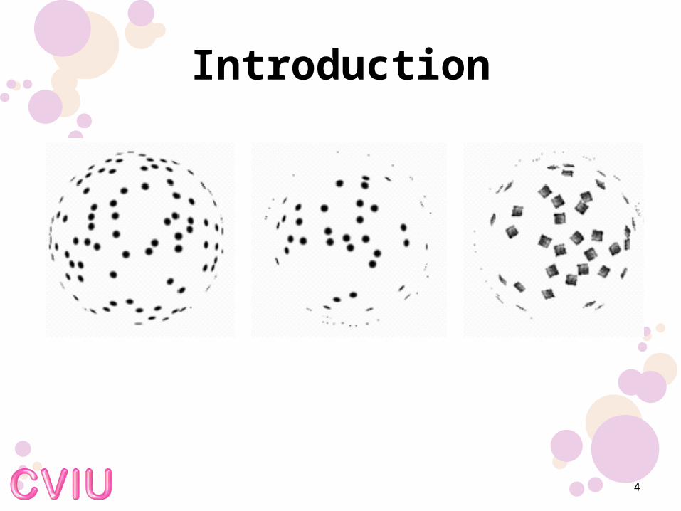
Introduction
4

General Ideas
• Tokens– Whatever we need to group (pixels, points, surface
elements, etc., etc.)
• Top down segmentation– Tokens belong together because they lie on the
same object
• Bottom up segmentation– Tokens belong together because they are locally
coherent
5

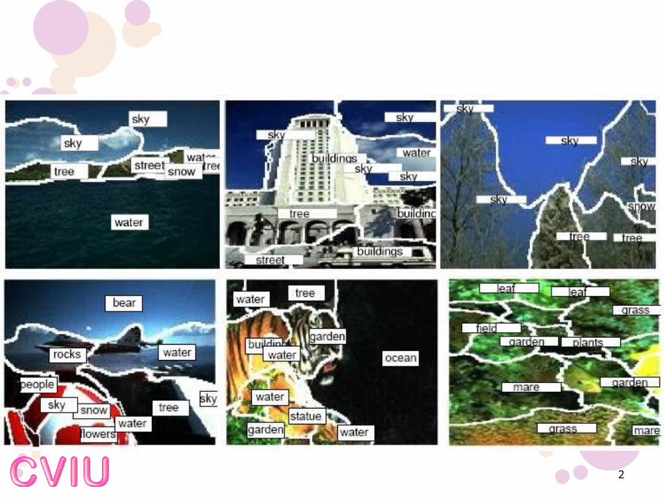
• Why & What is segmentation– Emphasize the property– Make main idea interesting– There are too many pixels in a single image– We need some form of compact, summary
representation
6

• What segmentation can do– Summarizing video– Finding machined parts– Finding people– Finding buildings in satellite
images– Searching a collection of images
7

• Model Problems– Forming image segments
• Roughly coherent color and texture
– Finding body segments• Arms, torso, etc.
– Fitting lines to edge points• To fit a line to a set of points
8

Segmentation as Clustering
• Partitioning– Decompose an image into regions– Decompose an image into extended blobs– Take a video sequence and decompose it into shots
• Grouping
9

Human Vision & Gestalt Properties
10

• Figure-ground discrimination– Grouping can be seen in terms of allocating some
elements to a figure, some to ground– Can be based on local bottom-up cues or high level
recognition
11

• Figure-ground discrimination
12

• A series of factors affect whether elements should be grouped together
13

• A series of factors affect whether elements should be grouped together
14

15

16

• Grouping by occlusions
17

• Grouping by invisible completions
18

Outline
• Introduction• Human Vision & Gestalt Properties• Applications
– Background Subtraction– Shot Boundary Detection
• Segmentation by Clustering– Simple Clustering Methods– K-means
• Segmentation by Graph-Theoretic Clustering– The Overall Approach– Affinity Measures– Normalized Cut
19

ApplicationBackground Subtraction
• Anything that doesn’t look like a known background is interesting
20

• Take a picture?• Not good…• The background changes slowly overtime…
21

• Estimate the value of background pixels using a moving average.
• Ideally, the moving average should track the changes in the background.
22

23

Shot Boundary Detection
• Where substantial changes in a video are interesting.
24

25

• Computing distance– Frame differencing
– Histogram-based
– Block comparison
– Edge differencing
pixel-by-pixel
histogram-by-histogram
box-by-box
edge map-by-edge map
26

Outline
• Introduction• Human Vision & Gestalt Properties• Applications
– Background Subtraction– Shot Boundary Detection
• Segmentation by Clustering– Simple Clustering Methods– K-means
• Segmentation by Graph-Theoretic Clustering– The Overall Approach– Affinity Measures– Normalized Cut
27

Segmentation by Clustering Simple Clustering Methods
• Divisive clustering
28

• Divisive clustering
29
p, q, r, s, t
r, s, t
p, q
qp r
s, t
s t

• Agglomerative clustering
30

• Agglomerative clustering
31
p, q, r, s, t
qp
p, q
r
r, s, t
s t
s, t

• Q: what the distance of A:
32
( , ) ( , )s q q sd C C d C C
( , ) ( ( , ), ( , ), ( , ))q s i s j s i jd C C f d C C d C C d C C

• Single-link clustering
33
( , ) min{ ( , ), ( , )}q s i s j sd C C d C C d C C

• Complete-link clustering
34
( , ) max{ ( , ), ( , )}q s i s j sd C C d C C d C C

• Group average clustering
( , ) { ( , ), ( , )}q s i s j sd C C avg d C C d C C
35

K-means
36

37
37
-2 -1.5 -1 -0.5 0 0.5 1 1.5 2
0
0.5
1
1.5
2
2.5
3
x
y
Iteration 1
-2 -1.5 -1 -0.5 0 0.5 1 1.5 2
0
0.5
1
1.5
2
2.5
3
x
y
Iteration 2
-2 -1.5 -1 -0.5 0 0.5 1 1.5 2
0
0.5
1
1.5
2
2.5
3
x
y
Iteration 3
-2 -1.5 -1 -0.5 0 0.5 1 1.5 2
0
0.5
1
1.5
2
2.5
3
x
y
Iteration 4
-2 -1.5 -1 -0.5 0 0.5 1 1.5 2
0
0.5
1
1.5
2
2.5
3
x
y
Iteration 5
-2 -1.5 -1 -0.5 0 0.5 1 1.5 2
0
0.5
1
1.5
2
2.5
3
x
y
Iteration 6

38

Outline
• Introduction• Human Vision & Gestalt Properties• Applications
– Background Subtraction– Shot Boundary Detection
• Segmentation by Clustering– Simple Clustering Methods– K-means
• Segmentation by Graph-Theoretic Clustering– The Overall Approach– Affinity Measures– Normalized Cut
39

Segmentation by Graph-theoretic Clustering• Terminology for Graph
– Vertices– Edges
• Directed graph
• Undirected graph
• Weighted graph
• Self-loop
• Connected graph– Connected components
40
},{ EVG 4
2
3
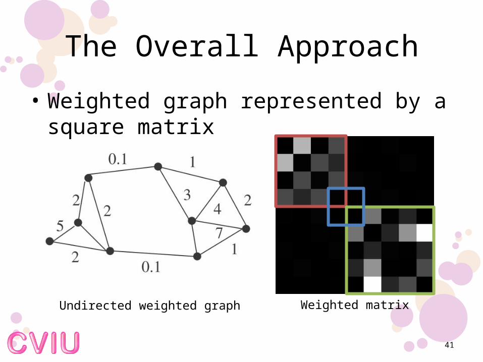
• Weighted graph represented by a square matrix
The Overall Approach
41
Undirected weighted graph Weighted matrix

42
Set of well separated points Affinity matrix

Affinity Measures
• Affinity by Distance
43
22
)()(exp),(
d
t yxyxyxaff
1.0d 2.0d 1d

• Affinity by Intensity
• Affinity by Color
• Affinity by Texture
44
22
))()(())()((exp),(
I
t yIxIyIxIyxaff
2
2
2
))(),((exp),(
c
ycxcdistyxaff
22
))()(())()((exp),(
I
t yfxfyfxfyxaff

Eigenvectors and segmentation
45
• Extracting a Single Good Cluster
{ association of element I with cluster n } ×{ affinity between I and j } ×
{ association of element j with cluster n}
nTn AwwA :Element affinities
nw :The vector of weight linking elements to the th clustern

46
• Scaling by scales• Normalizes the weights by requiring that
• Differentiation and dropping
)1( nTnn
Tn wwAww
nw :eigenvector of A
nn wAw
1nTn ww
nw
Lagrangia
n

47
Small2.0d

• Extracting Weights for a Set of Clusters– quite tight– distinct.
48
The three largest eigenvalues of the affinity matrix for the dataset

49
1.0d 2.0d 1d

Outline
• Introduction• Human Vision & Gestalt Properties• Applications
– Background Subtraction– Shot Boundary Detection
• Segmentation by Clustering– Simple Clustering Methods– K-means
• Segmentation by Graph-Theoretic Clustering– The Overall Approach– Affinity Measures– Normalized Cut
50

Normalized Cut
51
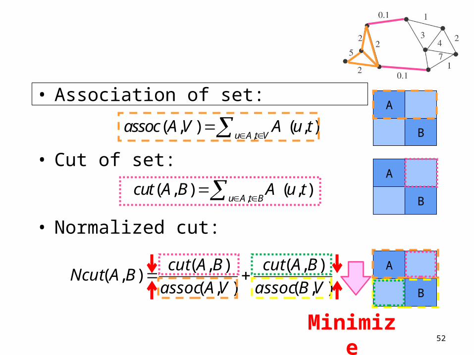
• Association of set:
),(
),(
),(
),(),(
VBassoc
BAcut
VAassoc
BAcutBANcut
,( , ) ( , )
u A t Vassoc A V u t
A
A
B
52
• Normalized cut:
• Cut of set:
,( , ) ( , )
u A t Bcut A B u t
A
A
B
A
B
Minimize

• Minimize Ncut– Transform Ncut equation to a matrical form.
53
Dyy
yADyxNcut
T
T
yx
)(min)(min
: affinity matrix
: , 0( )
: a vector which is giving the association
between each element and a cluster
1 ,node belong to one cluster:
,node belong to the other
j
i
D Dii ij Dij i j
x
iy y
b i
A
A
0 5 2 0 0 0 0 0 05 0 1 2 0 0 0 0 02 1 0 2 0 0 .1 0 00 2 2 0 .1 0 0 0 00 0 0 .1 0 3 0 1 00 0 0 0 3 0 1 4 70 0 .1 0 0 1 0 0 10 0 0 0 1 4 0 0 20 0 0 0 0 7 1 2 0
7 0 0 0 0 0 0 0 00 8 0 0 0 0 0 0 00 0 4. 0 0 0 0 0 00 0 0 4. 0 0 0 0 00 0 0 0 4. 0 0 0 00 0 0 0 0 15 0 0 00 0 0 0 0 0 5. 0 00 0 0 0 0 0 0 7 00 0 0 0 0 0 0 0 10
NP-Hard!
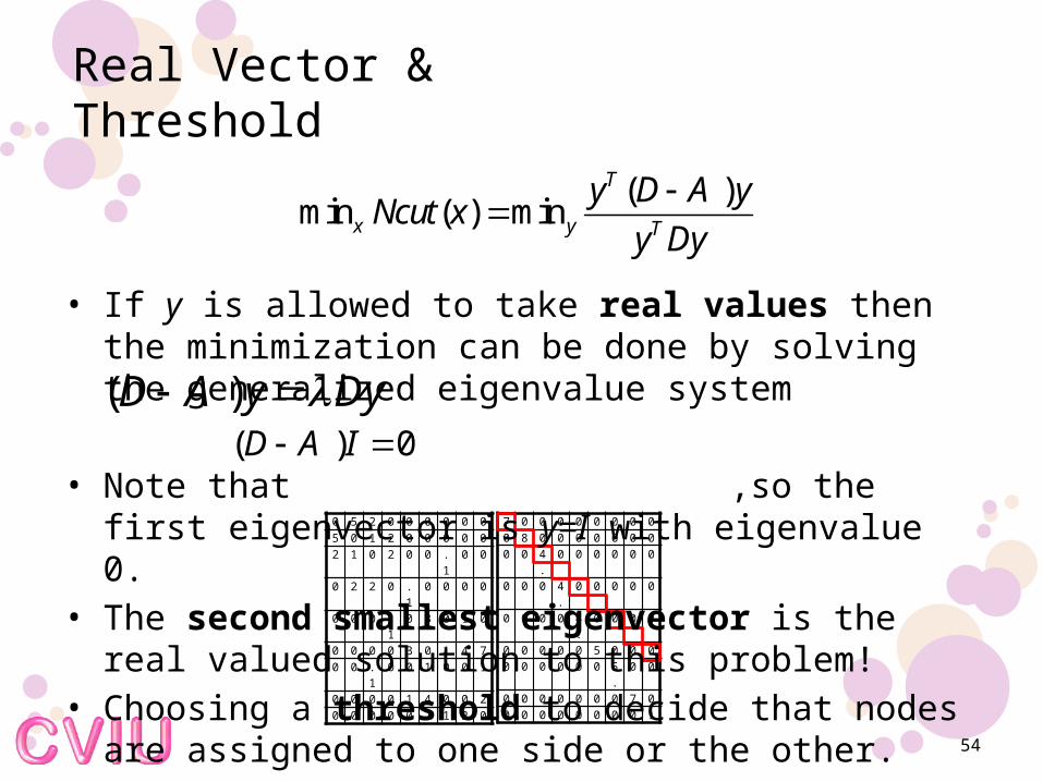
Real Vector & Threshold
54
( )min ( ) min
T
x y T
y D yNcut x
y Dy
A
( )D y Dy A( ) 0D I A
0 5 2 0 0 0 0 0 0
5 0 1 2 0 0 0 0 0
2 1 0 2 0 0 .1 0 0
0 2 2 0 .1 0 0 0 0
0 0 0 .1 0 3 0 1 0
0 0 0 0 3 0 1 4 7
0 0 .1 0 0 1 0 0 1
0 0 0 0 1 4 0 0 2
0 0 0 0 0 7 1 2 0
7 0 0 0 0 0 0 0 0
0 8 0 0 0 0 0 0 0
0 0 4. 0 0 0 0 0 0
0 0 0 4. 0 0 0 0 0
0 0 0 0 4. 0 0 0 0
0 0 0 0 0 5 0 0 0
0 0 0 0 0 0 5. 0 0
0 0 0 0 0 0 0 7 0
0 0 0 0 0 0 0 0 1
• If y is allowed to take real values then the minimization can be done by solving the generalized eigenvalue system
• Note that ,so the first eigenvector is y=I with eigenvalue 0.
• The second smallest eigenvector is the real valued solution to this problem!
• Choosing a threshold to decide that nodes are assigned to one side or the other.

Summarize
1. Define a similarity function between 2 nodes.
2. Compute affinity matrix (A) and degree matrix (D).
3. Solve
4. Use the eigenvector with the second smallest eigenvalue to bipartition the graph.
5. Recursively partition the segmented parts if necessary.
( )D y Dy A
55

Example
56

57

Thank you
58