chapter 11 regression and correlation methods. abdus wahed biost 2041 3 goals to relate (associate)...
TRANSCRIPT
Chapter 11
Regression and correlation methods
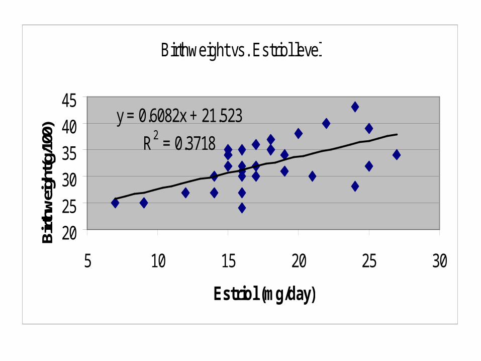
Birthweight vs. Estriol level
y = 0.6082x + 21.523
R2 = 0.3718
20
25
30
35
40
45
5 10 15 20 25 30
Estriol (mg/day)
Birth
wei
ght(g
/100
)
Abdus Wahed BIOST 2041
3
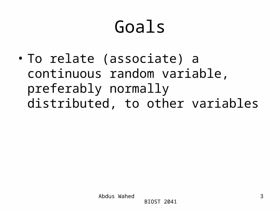
Goals
• To relate (associate) a continuous random variable, preferably normally distributed, to other variables
Abdus Wahed BIOST 2041
4
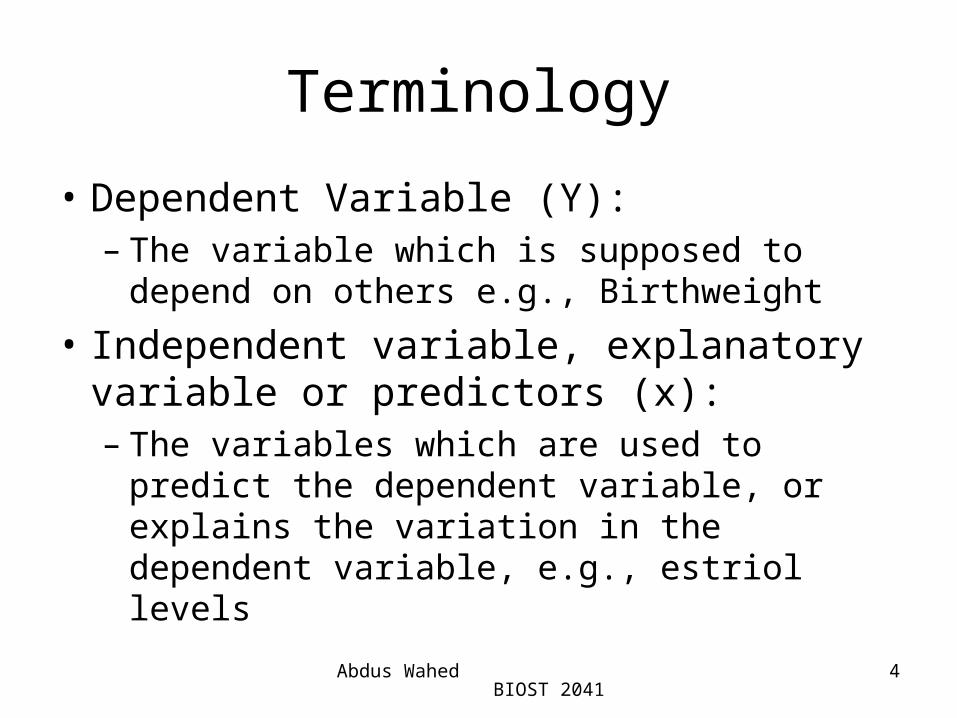
Terminology
• Dependent Variable (Y):– The variable which is supposed to depend on
others e.g., Birthweight
• Independent variable, explanatory variable or predictors (x):– The variables which are used to predict the
dependent variable, or explains the variation in the dependent variable, e.g., estriol levels
Abdus Wahed BIOST 2041
5
Assumptions
• Dependent Variable:– Continuous, preferably normally distributed– Have a linear association with the predictors
• Independent variable:– Fixed (not random)
Abdus Wahed BIOST 2041
6
Simple Linear Regression Model
• Assume Y be the dependent variable and x be the lone covariate. Then a linear regression assumes that the true relationship between Y and x is given by
E(Y|x) = α + βx (1)
Abdus Wahed BIOST 2041
7
Simple Linear Regression Model
• (1) can be written as
Y = α + βx + e, (2)
where
e is an error term with mean 0 and variance σ2.

Birthweight vs. Estriol level
y = 0.6082x + 21.523
R2 = 0.3718
20
25
30
35
40
45
5 10 15 20 25 30
Estriol (mg/day)
Birth
wei
ght(g
/100
)
ee

Abdus Wahed BIOST 2041
9
Implication
• If there was a perfect linear relationship, every subject with the same value of x would have a common value of Y.– Deterministic relationship
• The error term takes into account the inter-patient variability.
• σ2 = Var(Y) = Var(e).
Abdus Wahed BIOST 2041
10
Parameters
α is the intercept of the line.β is the slope of the line, referred to as
regression coefficient o β < 0 indicates a negative linear association (the
higher the x, the smaller the Y)o β = 0, no linear relationship.o β > 0 indicates a positive linear association (the
higher the x, the larger the Y)o β is the amount of change in Y for a unit change in x.
Abdus Wahed BIOST 2041
11
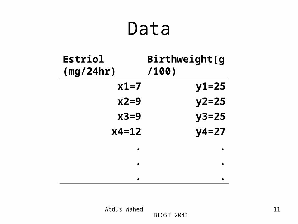
Data
Estriol (mg/24hr)
Birthweight(g/100)
x1=7 y1=25
x2=9 y2=25
x3=9 y3=25
x4=12 y4=27
. .
. .
. .

Abdus Wahed BIOST 2041
12
Goal
• How to estimate α, β, and σ2?– Fitting Regression Lines
• How to draw inference? The relationship we see – is it just due to chance?– Inference about regression parameters
Abdus Wahed BIOST 2041
13
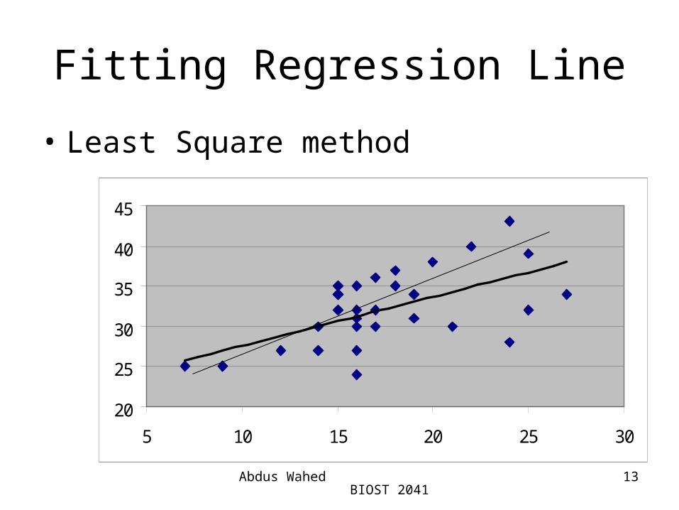
Fitting Regression Line
• Least Square method
20
25
30
35
40
45
5 10 15 20 25 30
Abdus Wahed BIOST 2041
14
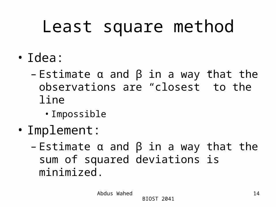
Least square method
• Idea:– Estimate α and β in a way that the
observations are “closest” to the line• Impossible
• Implement:– Estimate α and β in a way that the sum of
squared deviations is minimized.
Abdus Wahed BIOST 2041
15
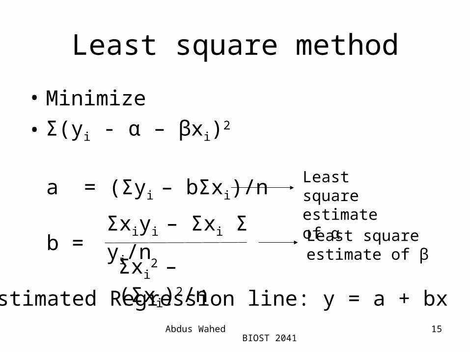
Least square method
• Minimize
• Σ(yi - α – βxi)2
b =Σxiyi – Σxi Σ yi/n
Σxi2
–(Σxi)2/n
a = (Σyi – bΣxi)/n Least square estimate of α
Least square estimate of β
Estimated Regression line: y = a + bx
Abdus Wahed BIOST 2041
16
Example 11.3
• Estimate the regression line for the birthweight data in Table 11.1, i.e.
• Estimate the intercept a and slope b
• We do the following calculations (see the corresponding Excel file)
Abdus Wahed BIOST 2041
17
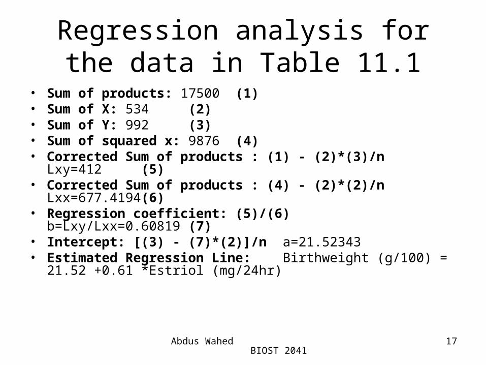
Regression analysis for the data in Table 11.1
• Sum of products: 17500 (1)• Sum of X: 534 (2)• Sum of Y: 992 (3)• Sum of squared x: 9876 (4)• Corrected Sum of products : (1) - (2)*(3)/n
Lxy=412 (5)• Corrected Sum of products : (4) - (2)*(2)/n
Lxx=677.4194 (6)• Regression coefficient: (5)/(6)
b=Lxy/Lxx=0.60819 (7)• Intercept: [(3) - (7)*(2)]/n
a=21.52343• Estimated Regression Line: Birthweight
(g/100) = 21.52 +0.61 *Estriol (mg/24hr)

Abdus Wahed BIOST 2041
18
Regression Analysis: Interpretation
• There is a positive association (statistically significant or not, we will test later) between birthweight and estriol levels.
• For each mg increase in estriol level, the birthweight of the newborn is increased by 61 g.
Abdus Wahed BIOST 2041
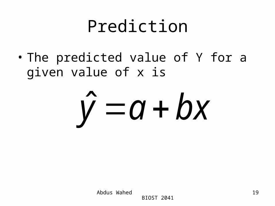
19
• The predicted value of Y for a given value of x is
Prediction
bxay ˆ

Abdus Wahed BIOST 2041
20
Prediction
• What is the estimated (predicted) birthweight if a pregnant women has an estriol level of 15 mg/24hr?
15*608.052.21ˆ y= 30.65 (g/100) = 3065 g

Abdus Wahed BIOST 2041
21
Calibration
• If low birthweight is defined as <= 2500, for what estriol level would the newborn be low birthweight?
• That is to what value of estriol level does the predicted birthweight of 2500 correspond to?
?*25 ba

Abdus Wahed BIOST 2041
22
Calibration
x608.052.2125 72.5608.0/)52.2125( x
Women having estriol level of 5.72 or lower are expected to have low birthweight newborns
Abdus Wahed BIOST 2041
23
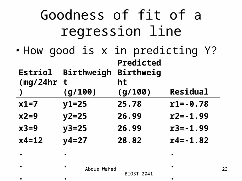
Goodness of fit of a regression line
• How good is x in predicting Y?
Estriol (mg/24hr)
Birthweight(g/100)
PredictedBirthweight(g/100) Residual
x1=7 y1=25 25.78 r1=-0.78
x2=9 y2=25 26.99 r2=-1.99
x3=9 y3=25 26.99 r3=-1.99
x4=12 y4=27 28.82 r4=-1.82
. . .
. . .
. . .

Abdus Wahed BIOST 2041
24
Goodness of fit of a regression line
• Residual sum of squares (Res SS)2)ˆ(.Re ii
i
yySSs Summary Measure of Distance Between the Observed and Predicted
The smaller the Res. SS, the better the regression line is in predicting Y
Abdus Wahed BIOST 2041
25
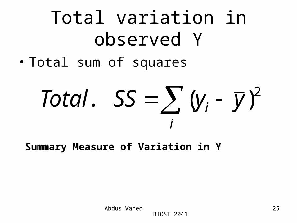
Total variation in observed Y
• Total sum of squares
2)(. yySSTotal ii
Summary Measure of Variation in Y

Abdus Wahed BIOST 2041
26
Total variation in predicted Y
• Total sum of squares
2)ˆ(.Re yySSg ii
Summary Measure of Variation in predicted Y

Abdus Wahed BIOST 2041
27
Goodness of fit of a regression line
yy
yyi
ii
i
ˆ
ˆ
Abdus Wahed BIOST 2041
28
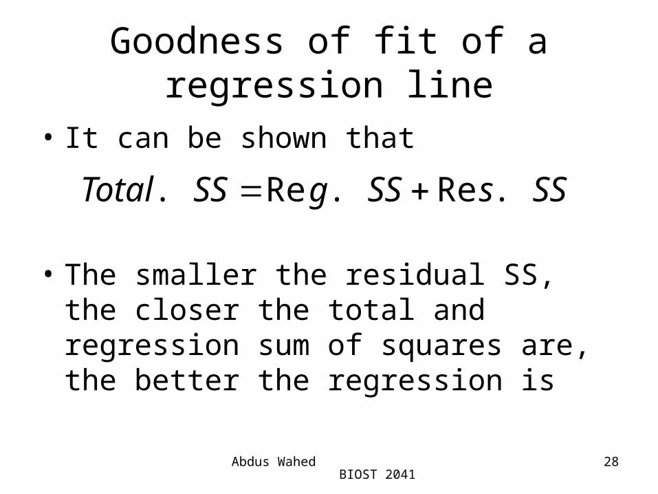
Goodness of fit of a regression line
• It can be shown that
• The smaller the residual SS, the closer the total and regression sum of squares are, the better the regression is
SSsSSgSSTotal .Re.Re.

Abdus Wahed BIOST 2041
29
Coefficient of determination R2
SSTotal
SSgR
.Re2
R2 is the proportion of total variation in Y explained bythe regression on x.
R2 lies between 0 and 1.
R2 = 1 implies a perfect fit (all the points are on the line).
Abdus Wahed BIOST 2041
30
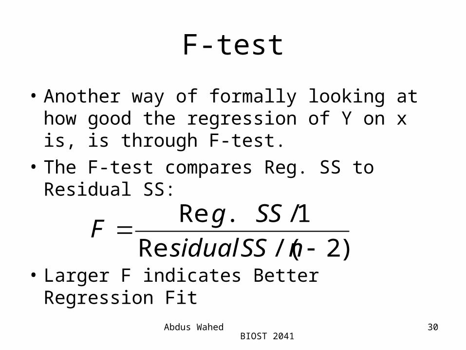
F-test
• Another way of formally looking at how good the regression of Y on x is, is through F-test.
• The F-test compares Reg. SS to Residual SS:
• Larger F indicates Better Regression Fit
)2/(Re
1/.Re
nSSsidual
SSgF

Abdus Wahed BIOST 2041
31
F-test
• Test
• Test statistic
• Reject H0 if F > F1,n-2,1-α
02,1~)2/(Re
1/.ReHunderF
nSSsidual
SSgF n
0:
.0:
1
0
H
vsH

Abdus Wahed BIOST 2041
32
Summary of Goodness of regression fit
• We need to compute three quantities– Total SS– Reg. SS– Res. Ss
• Total SS = Lyy
• Reg. SS = b*Lxy
• Res. SS = Total SS – Reg.SS

Abdus Wahed BIOST 2041
33
Example 11.12
• Total SS : 674• Reg. SS : 250.57• R^2 : 0.37 => 37% of the variation in
birthweight is explained by the regression on estriol level
• F :17.16• p-value : P(F1,29 > 17.16) = 0.0003• H0 is rejected => The slope of the regression
line is significantly different from zero, implying a statistically significant linear relationship between estriol level and birthweight
Abdus Wahed BIOST 2041
34
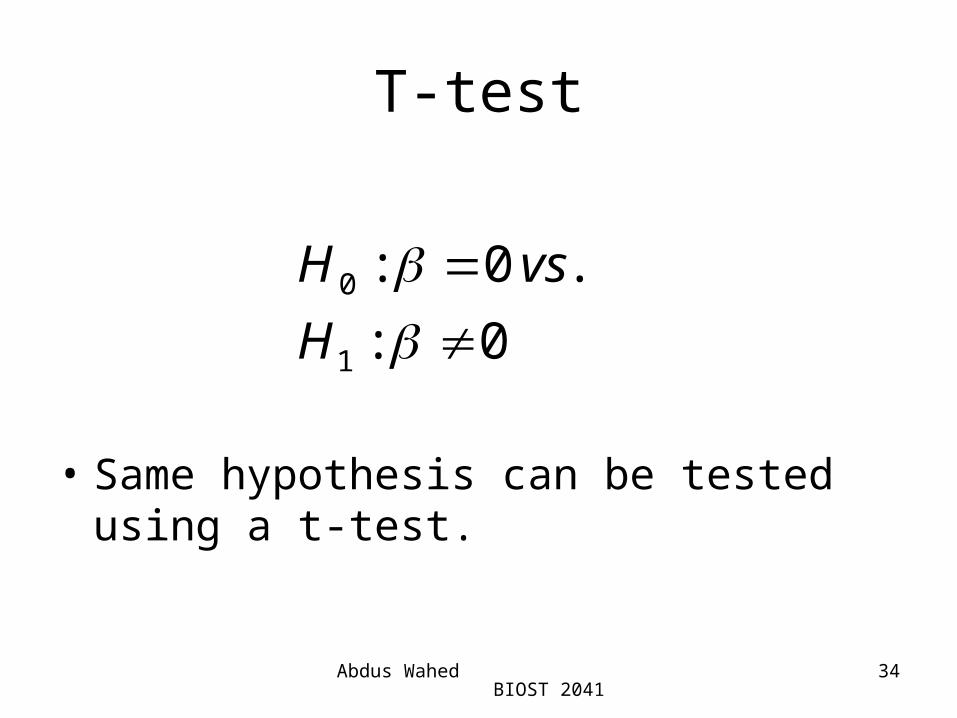
T-test
• Same hypothesis can be tested using a t-test.
0:
.0:
1
0
H
vsH
Abdus Wahed BIOST 2041
35
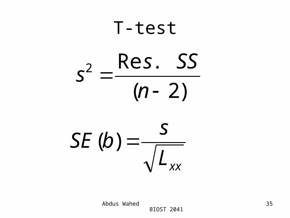
T-test
)2(
.Re2
n
SSss
xxL
sbSE )(
Abdus Wahed BIOST 2041
36
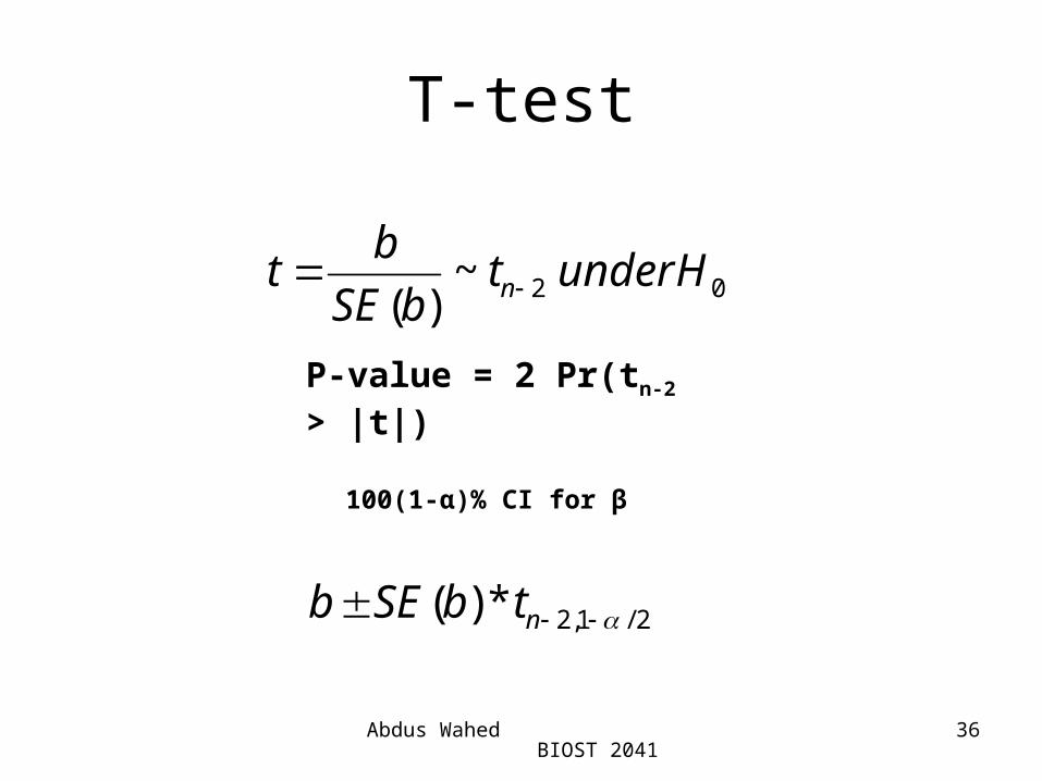
T-test
02~)(
HundertbSE
bt n
P-value = 2 Pr(tn-2 > |t|)
2/1,2*)( ntbSEb
100(1-α)% CI for β

Abdus Wahed BIOST 2041
37
Example 11.12
• Is the regression coefficient (slope) for the estriol level significantly different from zero?
• S^2= 14.6 s= 3.82• SE(b)= 0.15 t= 4.14• p= 0.00027123• 95% CI for reg coeff (0.31, 0.91)• H0: β = 0 is rejected => The slope of the regression line
is significantly different from zero, implying a statistically significant linear relationship between estriol level and birthweight
Abdus Wahed BIOST 2041
38
Correlation
• Correlation refers to a quantitative measure of the strength of linear relationship between two variables
• Regression, on the other hand is used for prediction
• No distinction between dependent and independent variable is made when assessing the correlation
Abdus Wahed BIOST 2041
39
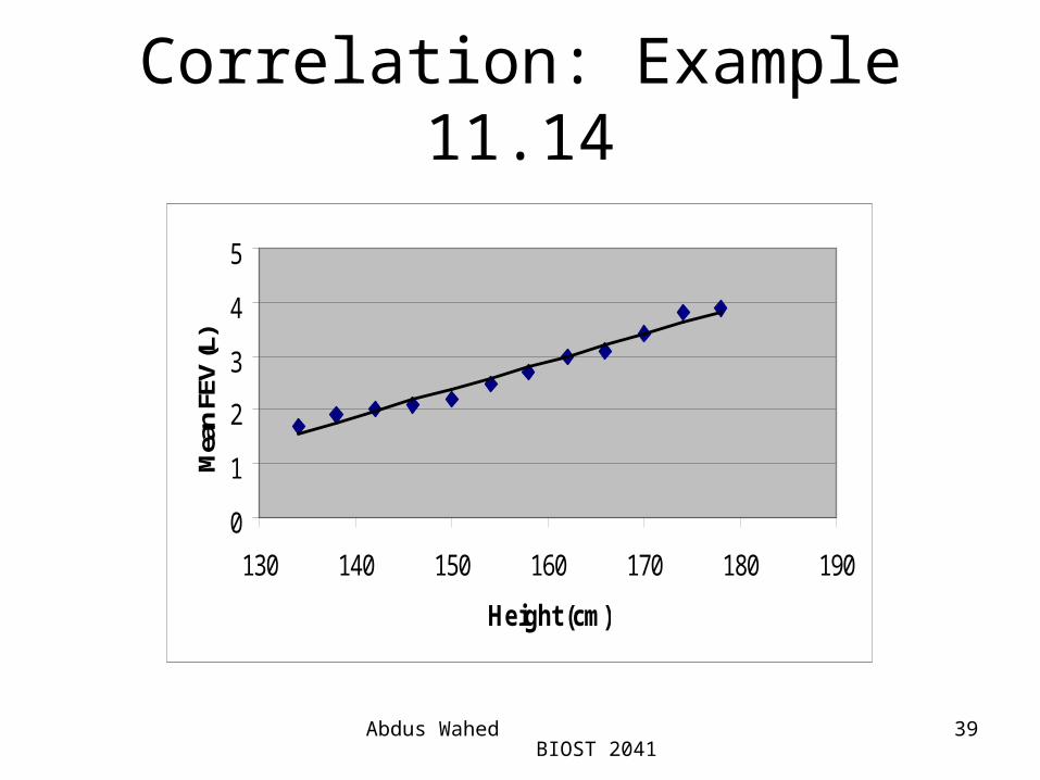
Correlation: Example 11.14
0
1
2
3
4
5
130 140 150 160 170 180 190
Height (cm)
Mea
n FE
V (L
)

Abdus Wahed BIOST 2041
40
Correlation
130
140
150
160
170
180
190
0 2 4 6 8 10 12 14
Mean FEV (L)
Hei
gh
t
Abdus Wahed BIOST 2041
41
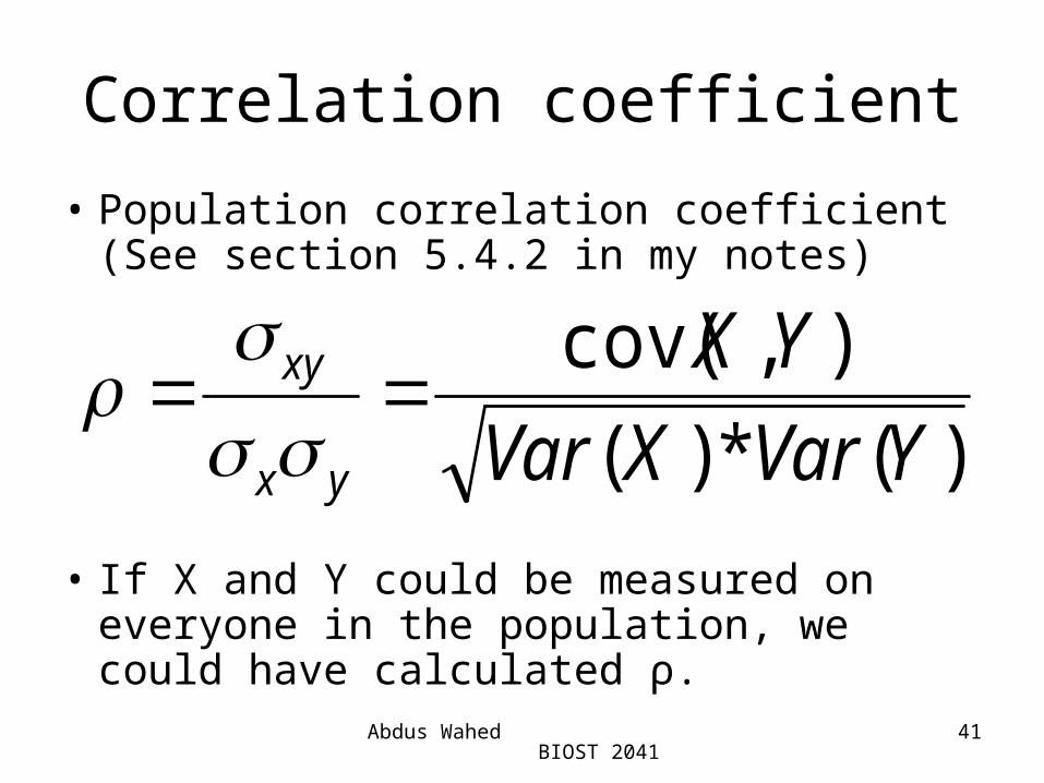
Correlation coefficient
• Population correlation coefficient (See section 5.4.2 in my notes)
• If X and Y could be measured on everyone in the population, we could have calculated ρ.
)(*)(
),cov(
YVarXVar
YX
yx
xy
Abdus Wahed BIOST 2041
42
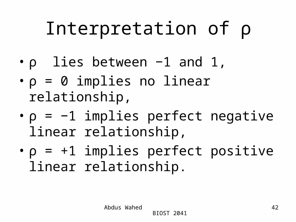
Interpretation of ρ
• ρ lies between −1 and 1,
• ρ = 0 implies no linear relationship,
• ρ = −1 implies perfect negative linear relationship,
• ρ = +1 implies perfect positive linear relationship.
Abdus Wahed BIOST 2041
43
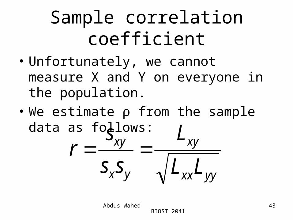
Sample correlation coefficient
• Unfortunately, we cannot measure X and Y on everyone in the population.
• We estimate ρ from the sample data as follows:
yyxx
xy
yx
xy
LL
L
ss
sr

Abdus Wahed BIOST 2041
44
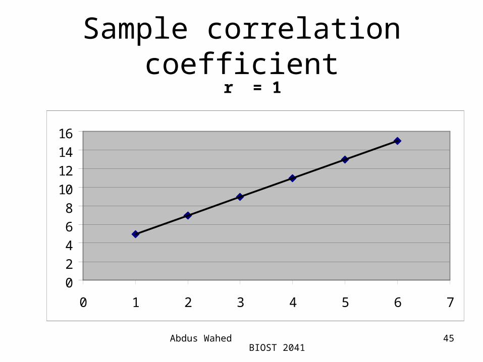
Interpretation of r
• r lies between −1 and 1,
• r = 0 implies no linear relationship,
• r = −1 implies perfect negative linear relationship,
• r = +1 implies perfect positive linear relationship,
• The closer |r| is to 1, the stronger the relationship is.
Abdus Wahed BIOST 2041
45
Sample correlation coefficient
0
2
4
6
8
10
12
14
16
0 1 2 3 4 5 6 7
r = 1

Abdus Wahed BIOST 2041
46
Sample correlation coefficientr = -1
0
2
4
6
8
10
12
14
0 1 2 3 4 5 6 7

Abdus Wahed BIOST 2041
47
Sample correlation coefficient
0
1
2
3
4
5
6
0 1 2 3 4 5 6 7
r=0

Abdus Wahed BIOST 2041
48
Sample correlation coefficient
00.5
11.5
22.5
33.5
44.5
130 140 150 160 170 180 190
r=0.988
Abdus Wahed BIOST 2041
49
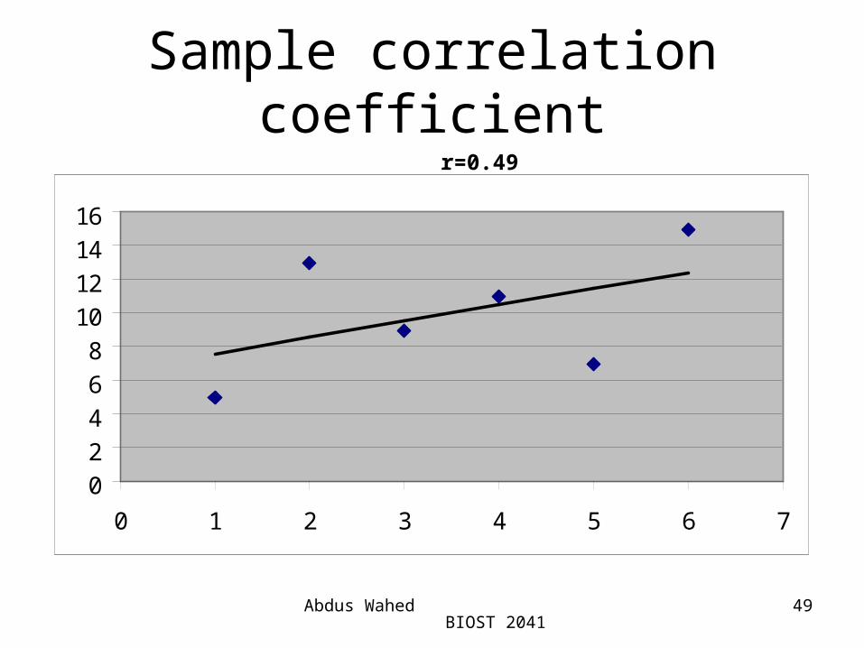
Sample correlation coefficient
0
2
4
6
8
10
12
14
16
0 1 2 3 4 5 6 7
r=0.49

Abdus Wahed BIOST 2041
50
Sample correlation coefficientr=-0.37
0
2
4
6
8
10
12
14
0 1 2 3 4 5 6 7

Abdus Wahed BIOST 2041
51
Correlation: Example 11.14
• Sum of products: 5156.2 (1)• Sum of X: 1872 (2)• Sum of Y: 32.3 (3)• Sum of squared X: 294320 (4)• Sum of squared Y: 93.11 (5)• Corrected Sum of products : (1) - (2)*(3)/n
Lxy = 117.4 (6)• Corrected Sum of squares of X : (4) - (2)*(2)/n
Lxx = 2288 (7)• Corrected Sum of squares of Y : (5) - (3)*(3)/n
Lyy = 6.17 (8)• Sample Correlation Coefficient (6)/sqrt[(7)*(8)]
r = 0.988
Abdus Wahed BIOST 2041
52
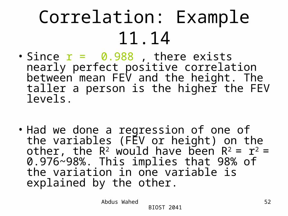
Correlation: Example 11.14
• Since r = 0.988 , there exists nearly perfect positive correlation between mean FEV and the height. The taller a person is the higher the FEV levels.
• Had we done a regression of one of the variables (FEV or height) on the other, the R2 would have been R2 = r2 = 0.976~98%. This implies that 98% of the variation in one variable is explained by the other.

Abdus Wahed BIOST 2041
53
Correlation: Example 11.24
• The sample correlation coefficient between estriol levels and the birth weights is calculated as r = 0.61, implying moderately strong positive linear relationship. The higher the estriol levels, the higher the birth weights.
• Remember, R2 = 0.37 (slide # 33) which is equal to r2 = (0.61)2.
Abdus Wahed BIOST 2041
54
Statistical Significance of Correlation
• If |r| is close to 1, such as 0.988, one would believe that there is a strong linear relationship between the two variables. That means, there is no reason to believe that this strong association just happened by chance (sampling/observation).
Abdus Wahed BIOST 2041
55
Statistical Significance of Correlation
• But If |r| = 0.23, what conclusion would you draw about the relationship? Is it possible that in truth there was no correlation (ρ = 0), but the sample by chance only shows that there is some sort of correlation between the two variables?
Abdus Wahed BIOST 2041
56
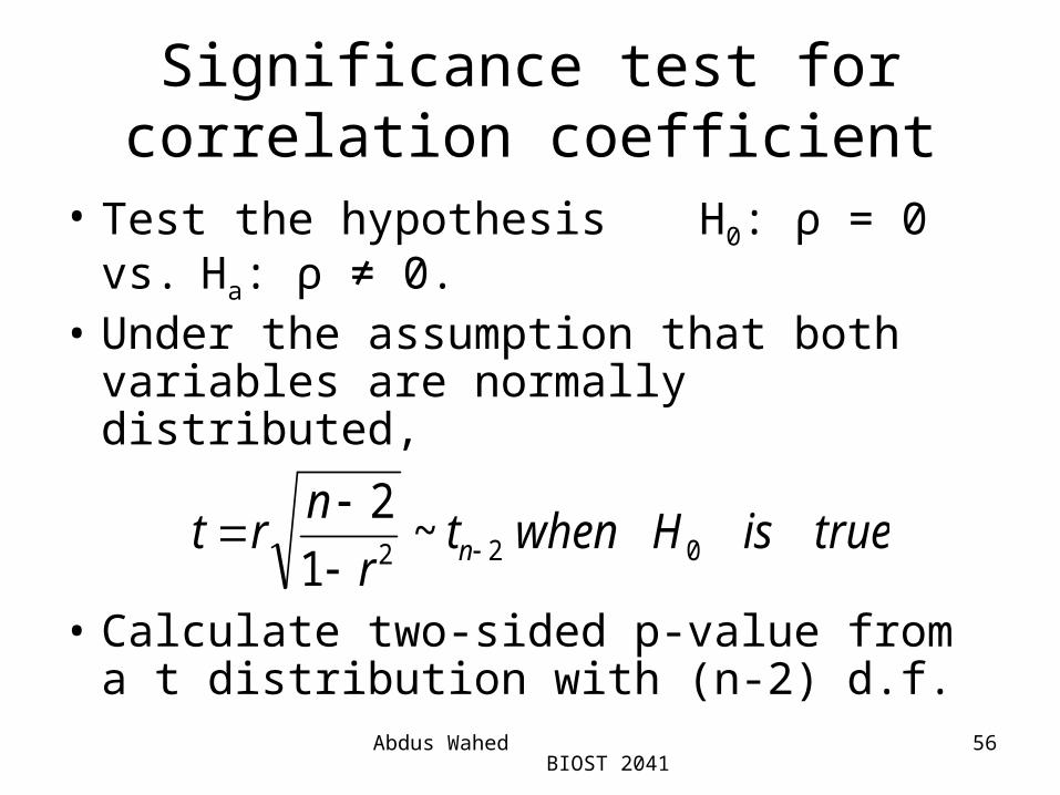
Significance test for correlation coefficient
• Test the hypothesisH0: ρ = 0 vs.Ha: ρ ≠ 0.
• Under the assumption that both variables are normally distributed,
• Calculate two-sided p-value from a t distribution with (n-2) d.f.
trueisHwhentr
nrt n 022
~1
2
Abdus Wahed BIOST 2041
57
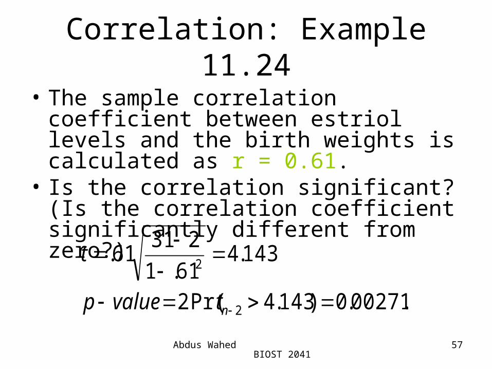
Correlation: Example 11.24
• The sample correlation coefficient between estriol levels and the birth weights is calculated as r = 0.61.
• Is the correlation significant? (Is the correlation coefficient significantly different from zero?)
.00271.0)143.4Pr(2
143.461.1
23161.
2
2
ntvaluep
t
Abdus Wahed BIOST 2041
58
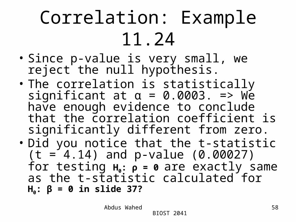
Correlation: Example 11.24
• Since p-value is very small, we reject the null hypothesis.
• The correlation is statistically significant at α = 0.0003. => We have enough evidence to conclude that the correlation coefficient is significantly different from zero.
• Did you notice that the t-statistic (t = 4.14) and p-value (0.00027) for testing H0: ρ = 0 are exactly same as the t-statistic calculated for H0: β = 0 in slide 37?
Abdus Wahed BIOST 2041
59
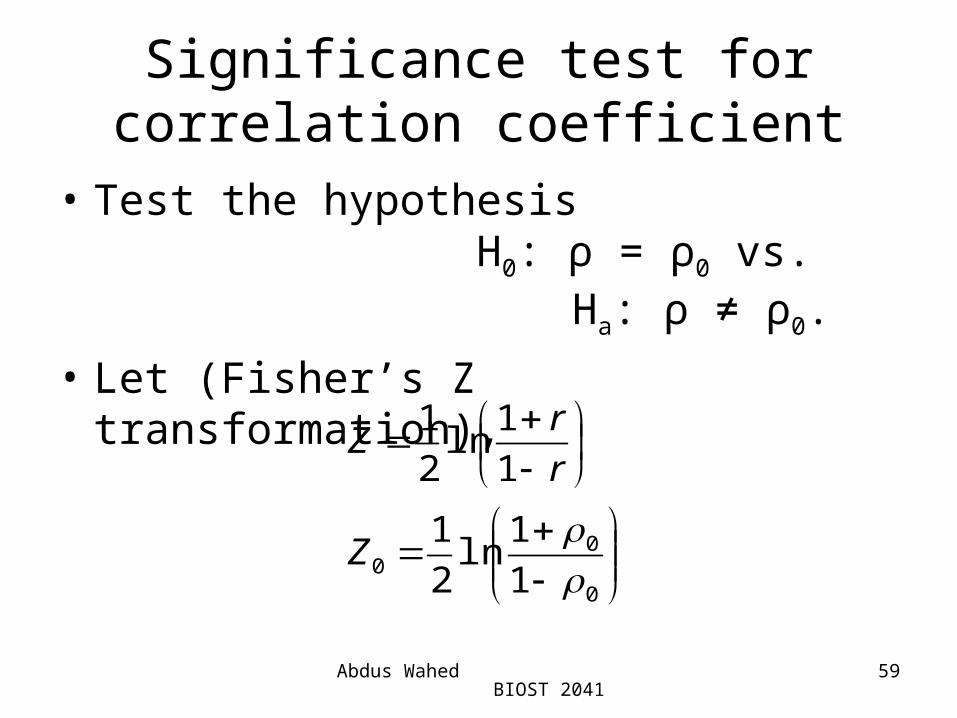
Significance test for correlation coefficient
• Test the hypothesisH0: ρ = ρ0 vs.Ha: ρ ≠ ρ0.
• Let (Fisher’s Z transformation),
0
00 1
1ln2
1
1
1ln2
1
Z
r
rZ
Abdus Wahed BIOST 2041
60
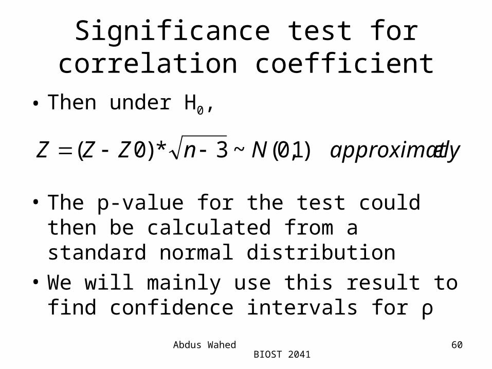
Significance test for correlation coefficient
• Then under H0,
• The p-value for the test could then be calculated from a standard normal distribution
• We will mainly use this result to find confidence intervals for ρ
elyapproximatNnZZZ )1,0(~3*)0(
Abdus Wahed BIOST 2041
61
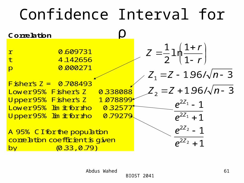
Confidence Interval for ρCorrelation
r 0.609731t 4.142656p 0.000271
Fisher's Z = 0.708493Lower 95% Fisher's Z 0.338088Upper 95% Fisher's Z 1.078899Lower 95% limit for rho 0.32577Upper 95% limit for rho 0.79279
A 95% CI for the population correlation coefficient is givenby (0.33, 0.79)
r
rZ
1
1ln2
1
3/96.1
3/96.1
2
1
nZZ
nZZ
1
1
1
1
2
2
1
1
2
2
2
2
Z
Z
Z
Z
e
e
e
e