chapter 11 car-following models based on driving...
TRANSCRIPT
Chapter 11Car-Following Models based on DrivingStrategies
Ideas are like children: you always love your own the most.Lothar Schmidt
Abstract The models introduced in this chapter are derived from assumptions aboutreal driving behavior such as keeping a “safe distance” fromthe leading vehicle,driving at a desired speed, or preferring accelerations to be within a comfortablerange. Additionally, kinematical aspects are taken into account, such as the quadraticrelation between braking distance and speed. We introduce two examples: The sim-plified Gipps model, and the Intelligent Driver Model. Both models use the sameinput variables as the sensors ofadaptive cruise control(ACC) systems, and pro-duce a similar driving behavior. Characteristics that are specific to the human nature,like erroneous judgement, reaction time, and multi-anticipation, are discussed in thenext chapter.
11.1 Model Criteria
The models introduced in this chapter are formally identical to the minimal modelspresented in the previous chapter. They are defined by an acceleration functionamic
(see Eq. (10.3)) or a speed functionvmic (see Eq. (10.7)). In contrast to the minimalmodels, the acceleration or speed functions encoding the driving behavior should atleast model the following aspects:
1. The acceleration is a strictly decreasing function of thespeed. Moreover, thevehicle accelerates towards adesired speed v0 if not constrained by other vehiclesor obstacles:
∂amic(s,v,vl )
∂v< 0, lim
s→∞amic(s,v0,vl ) = 0 for all vl . (11.1)
2. The acceleration is an increasing function of the distances to the leading vehicle:
∂amic(s,v,vl )
∂s≥ 0, lim
s→∞
∂amic(s,v,vl )
∂s= 0 for all vl . (11.2)
181
Sample Chapter from "Traffic Flow Dynamics" written by M.Treiber and A.KestingMore information: http://www.traffic-flow-dynamics.orgBy courtesy of Springer publisher, http://www.springer.com

182 11 Car-Following Models based on Driving Strategies
The inequality becomes an equality if other vehicles or obstacles (including “vir-tual” obstacles such as the stopping line at a red traffic light) are outside the in-teraction range and therefore do not influence the driving behavior. This definesthefree-flow acceleration
afree(v) = lims→∞
amic(s,v,vl ) =≥ amic(s,v,vl ). (11.3)
3. The acceleration is an increasing function of the speed ofthe leading vehicle.Together with requirement (1), this also means that the acceleration decreases(the deceleration increases) with the speed of approach to the lead vehicle (orobstacle):
∂ amic(s,v,∆v)∂∆v
≤ 0 or∂amic(s,v,vl )
∂vl≥ 0, lim
s→∞
∂amic(s,v,vl )
∂vl= 0. (11.4)
Again, the equality holds if other vehicles (or obstacles) are outside the interac-tion range.
4. A minimum gap (bumper-to-bumper distance)s0 to the leading vehicle is main-tained (also during a standstill). However, there is no backwards movement if thegap has become smaller thans0 by past events:
amic(s,0,vl ) = 0 for all vl ≥ 0, s≤ s0. (11.5)
By virtue of relation (10.11), these requirements (orplausibility conditions) for theacceleration function naturally imply conditions for the speed functionvmic of mod-els formulated in terms of coupled maps.
A car-following model meeting these requirements iscompletein the sense thatit can consistently describe all situations that may arise in single-lane traffic. Par-ticularly, it follows that (i) all vehicle interactions areof finite reach, (ii) followingvehicles are not “dragged along”,
amic(s,v,vl )≤ amic(∞,v,v′l ) = afree(v) for all s,v,vl , andv′l , (11.6)
and (iii) an equilibrium speedve(s) exists, which has the properties already postu-lated for the optimal-speed function (10.20):
v′e(s)≥ 0, ve(0) = 0, lims→∞
ve(s) = v0. (11.7)
This means that the model possesses a unique steady-state flow-density relation, i.e.,a fundamental diagram.1
These conditions are necessary but not sufficient. For example, when in the car-following regime (steady-state congested traffic), the time gap to the leader has toremain within reasonable bounds (say, between 0.5 s and 3 s).Furthermore, the ac-
1 If one were to weaken condition (11.1) to∂amic/∂v≤ 0, it is possible to formulate models thatdonot have a fundamental diagram. Such models are proposed in the context of B. Kerner’sthree-phase theory.

11.2 Gipps’ Model 183
celeration has to be constrained to a “comfortable” range (e.g.,±2m/s2), or at least,to physically possible values. Particularly, when approaching the leading vehicle,the quadratic relation between braking distance and speed has to be taken into ac-count. Finally, any car-following model should allow instabilities and thus the emer-gence of “stop-and-go” traffic waves, but should not produceaccidents, i.e., negativebumper-to-bumper gapss< 0.2
Which of the car-following models introduced in Chapter 10 satisfy the con-ditions (11.1) – (11.5)?
11.2 Gipps’ Model
Gipps’ model presented here is a modified version of the one described in his orig-inal publication. It is simplified, but conceptually unchanged. Although it producesan unrealistic acceleration profile, this model is probablythe simplest complete andaccident-free model that leads to accelerations within a realistic range.
11.2.1 Safe Speed
Accidents are prevented in the model by introducing a “safe speed” vsafe(s,vl ),which depends on the distance to and speed of the leading vehicle. It is based onthe following assumptions:
1. Braking maneuvers are always executed with constant decelerationb. There isno distinction between comfortable and (physically possible) maximum deceler-ation.
2. There is a constant “reaction time”∆ t.3. Even if the leading vehicle suddenly decelerates to a complete stop (worst case
scenario), the distance gap to the leading vehicle should not become smaller thana minimum gaps0.3
Condition 1 implies that thebraking distancethat the leading vehicle needs to cometo a complete stop is given by
∆xl =v2
l
2b.
2 Traffic-flow models are meant to describenormalconditions, while accidents are almost alwayscaused byexceptionaldriving mistakes that are not part of normal driving behavior and thus notpart of the intended scope of the model.3 This condition is not present in the original paper, but is necessary to ensure an accident-freemodel in the presence of numerical errors arising from discretization.

184 11 Car-Following Models based on Driving Strategies
From condition 2 it follows that, in order to come to a complete stop, the driver ofthe considered vehicle needs not only his or her braking distancev2/(2b), but also anadditionalreaction distance v∆ t travelled during the reaction time.4 Consequently,thestopping distanceis given by
∆x= v∆ t +v2
2b. (11.8)
Finally, condition 3 is satisfied if the gaps exceeds the required minimum finalvalues0 by the difference∆x−∆xl between the stopping distance of the consideredvehicle and the breaking distance of the leader:
s≥ s0+v∆ t +v2
2b− v2
l
2b. (11.9)
The speedv for which the equal sign holds (the highest possible speed) defines the“safe speed”
vsafe(s,vl ) =−b∆ t +√
b2∆ t2+v2l +2b(s−s0). (11.10)
11.2.2 Model Equation
The simplified Gipps’ model is defined as an iterated map with the “safe speed” (11.10)as its main component:
v(t +∆ t) = min[v+a∆ t,v0,vsafe(s,vl )] Gipps’ model. (11.11)
This model equation reflects the following properties:
• The simulation update time step is equal to the reaction time∆ t.• If the current speed is greater thanvsafe−a ∆ t or v0−a ∆ t, the vehicle will reach
the minimum ofv0 andvsafeduring the next time step.5
• Otherwise the vehicle accelerates with constant acceleration a until either thesafe speed or the desired speed is reached.
11.2.3 Steady-State Equilibrium
The homogeneous steady state impliesv(t +∆ t) = vl = v, thus
4 In contrast to the original publication, we assume the speed to be constant within the reactiontime.5 Strictly speaking, this means that deceleration(v− vsafe)/∆ t is not restricted tob. In multi-lanesimulations, it can be greater if another vehicle “cuts in” in front of the considered vehicle.

11.2 Gipps’ Model 185
v= min(v0,vsafe) = min
(
v0,−b∆ t +√
b2∆ t2+v2+2b(s−s0)
)
,
which yields the steady-state speed-gap relation
ve(s) = max
[
0,min
(
v0,s−s0
∆ t
)]
(11.12)
and, assuming constant vehicle lengthsl , the familiar “triangular” fundamental dia-gram
Qe(ρ) = min
(
v0ρ ,1−ρ leff
∆ t
)
, (11.13)
whereleff = (l + s0). As in the Newell model, the parameter∆ t can be interpretedin four different ways: (i) As the reaction time introduced in the derivation ofvsafe,(ii) as the numerical update time step of the actual model equation (11.11), (iii) as aspeed adaption time in Eq. (11.11) (at least, ifv(t +∆ t) is restricted byvsafeor v0),or (iv) as the “safety time gap”(s−s0)/ve in congested traffic as deduced from thefundamental diagram (11.12).
Table 11.1 Parameters of the simplified Gipps’ model and typical values in different scenarios.
Parameter Typical Value Typical ValueHighway City Traffic
Desired speedv0 120 km/h 54 km/hAdaption/reaction time∆ t 1.1 s 1.1 sAccelerationa 1.5m/s2 1.5m/s2
Decelerationb 1.0m/s2 1.0m/s2
Minimum distances0 3 m 2 m
11.2.4 Model Characteristics
Unlike the minimal models described in the previous chapter, the Gipps’ modelis transparently derived from a few basic assumptions and uses parameters that areeasy to interpret and assign realistic values (Table 11.1).Furthermore, Gipps’ modelis – again, in contrast to the minimal models –robust in the sense that meaningfulresults can be produced from a comparatively wide range of parameter values.
Highway traffic. The simulation of the highway scenario (Fig. 11.1, left) producesmore realistic results than the OVM or the Newell model: The speed field in panel (a)exhibits small perturbations which are caused by vehicles merging from the on-ramp and grow into stop-and-go waves while propagating upstream. The propaga-tion velocity ccong= −leff/∆ t is constant and of the order of the empirical value

186 11 Car-Following Models based on Driving Strategies
V (km/h)
0 30 60 90
Time (min)
-8
-6
-4
-2
0
2
Dis
tanc
e fr
om o
nram
p (k
m)
0
20
40
60
80
100
120
140
0
500
1000
1500
2000
2500
0 20 40 60
Flo
w Q
(1/
h)
Density ρ (1/km)
-7 km-5 km-3 km-1 km
0
10
20
30
0 30 60 90 120 150
Gap
(m
)
Time (s)
Car 1Car 5
Car 10Car 15Car 20
(b)
(c)
(a)
0 10 20 30 40 50
0 30 60 90 120 150
Spe
ed (
km/h
)
Time (s)
Car 1Car 5
Car 10Car 15Car 20
(d)
-1
0
1
2
0 30 60 90 120 150
Acc
el. (
m/s
2 )
Time (s)
Car 1Car 5
Car 10Car 15Car 20
(e)
Fig. 11.1 Fact sheet of Gipps’ model (11.11),(11.10). Simulation of the two standard scenarios“highway” (left) and “city traffic” (right) with the parameter values listed in Table 11.1. See Chap-ter 10.5 for a detailed description of the scenarios.
(≈−15km/h). Furthermore, the wave length (of the order of 1−1.5km) is not toofar away from the empirical values (1.5−3km).
The flow-density diagram in Fig. 11.1(b), obtained from virtual detectors, showsa strongly scattered cloud of data points in the region of congested traffic, i.e., every-where to the right of the straight line indicating free traffic. Such a wide scatteringis in agreement with empirical data (cf. Figs. 4.11 and 4.12). By looking at scatterplots of individual detectors, one observes that detectorsthat are closer to the bot-tleneck produce data points that are shifted towards greater densities and closer tothe fundamental diagram of steady-state traffic. Moreover,the data points of virtualdetectors positioned inside the region of stationary traffic immediately upstream ofthe bottleneck (solid black squares) lie on the fundamentaldiagram itself. This ap-parent density increase near the outflow region of a congestion, also known aspincheffect, can be observed empirically. However, the systematic density underestima-tion, which conspicuously increases with the degree of the scattering of the datapoints, suggests that thereal density increase is smaller, or even nonexistent. Thismeans that the pinch effect is essentially a result of data misinterpretation, or, morespecifically, by estimating the density with the time mean speed instead of the spacemean speed (cf. Section 3.3.1). This interpretation is confirmed by simulation aswill be shown in Fig. 11.5(b) below. We draw an important conclusion that is notrestricted to Gipps’ model (and not even to traffic flow models):

11.3 Intelligent Driver Model 187
When using empirical data to assert the accuracy and predictive power ofmodels, one has to simulate both the actual traffic dynamicsand the processof data capture and analysis.
City traffic. Compared to the simple models of the previous chapter, the city-trafficscenario (Fig. 11.1, right column) is closer to reality as well. However, the accel-eration time-series is unrealistic. By definition, there are only three values for theacceleration: Zero,a, and−b (cf. Panel (e)). The resulting driving behavior is ex-cessively “robotic” and the abrupt transitions are unrealistic.
Moreover, Gipps’ model does not differentiate between comfortable and max-imum deceleration: Assuming thatb in Eq. (11.10) denotes the maximum decel-eration, the model is accident-free but every braking maneuver is performedveryuncomfortably with full brakes. On the other hand, when interpretingb as the com-fortable deceleration and allowing for heterogeneous and/or multi-lane traffic themodel possibly produces accidents if leading vehicles (which might be simulatedusing different parameters or even different models) brakeharder thanb.
In summary, Gipps’ model produces good results in view of itssimplicity. Mod-ified versions of this model are used in several commercial traffic simulators. Oneexample of such a modification isKrauss’ modelwhich essentially is a stochasticversion of the Gipps model.
11.3 Intelligent Driver Model
The time-continuousIntelligent Driver Model(IDM) is probably the simplest com-plete and accident-free model producing realistic acceleration profiles and a plausi-ble behavior in essentially all single-lane traffic situations.
11.3.1 Required Model Properties
As Gipps’ model, the IDM is derived from a list of basic assumptions (first-principles model). It is characterized by the following requirements:
1. The acceleration fulfills the general conditions (11.1) –(11.5) for a completemodel.
2. The equilibrium bumper-to-bumper distance to the leading vehicle is not lessthan a “safe distance”s0+vT wheres0 is a minimum (bumper-to-bumper) gap,andT the (bumper-to-bumper) time gap to the leading vehicle.
3. An braking strategy!intelligentcontrols how slower vehicles (or obstacles or redtraffic lights) are approached:

188 11 Car-Following Models based on Driving Strategies
• Under normal conditions, the braking maneuver is “soft”, i.e., the decelerationincreases gradually to a comfortable valueb, and decreases smoothly to zerojust before arriving at a steady-state car-following situation or coming to acomplete stop.
• In a critical situation, the deceleration exceeds the comfortable value untilthe danger is averted. The remaining braking maneuver (if applicable) will becontinued with the regular comfortable decelerationb.
4. Transitions between different driving modes (e.g., fromthe acceleration to thecar-following mode) are smooth. In other words, the time derivative of the ac-celeration function, i.e., thejerk J, is finite at all times.6 This is equivalent topostulating that the acceleration functionamic(s,v,vl ) (or amic(s,v,∆v)) is con-tinuously differentiable in all three variables. Notice that this postulate is in con-trast to the action-point models such as theWiedemann Modelwhere accelerationchanges are modeled as a series of discrete jumps.
5. The model should be as parsimonious as possible. Each model parameter shoulddescribe only one aspect of the driving behavior (which is favorable for modelcalibration). Furthermore, the parameters should correspond to an intuitive inter-pretation and assume plausible values.
11.3.2 Mathematical Description
The required properties are realized by the following acceleration equation:
v= a
[
1−(
vv0
)δ−(
s∗(v,∆v)s
)2]
IDM. (11.14)
The acceleration of the Intelligent Driver Model is given inthe formamic(s,v,∆v)and consists of two parts, one comparing the current speedv to the desired speedv0, and one comparing the current distances to the desired distances∗. The desireddistance
s∗(v,∆v) = s0+max
(
0,vT+v∆v
2√
ab
)
(11.15)
has an equilibrium terms0+vT and adynamical term v∆v/(2√
ab) that implementsthe “intelligent” braking strategy (see Section 11.3.4).7
6 Typical values of a “comfortable” jerk are|J| ≤ 1.5m/s3.7 The maximum condition in Eq. (11.15) ensures that the conditions (11.1) – (11.5) for modelcompleteness hold for all situations. Strictly speaking, this condition violates the postulate of asmooth acceleration function. However, it comes into effect only in two situations: (i) For finitespeeds if the leading car is much faster, (ii) for stopped queued vehicles when the queue starts tomove. The first situation may arise after a cut-in maneuver of a fastervehicle. Sinces≫ s0 for thiscase, the resulting discontinuity is small. In the second case, the maximum condition prevents anoverly sluggish start and the associated discontinuous acceleration profile may even be realistic.

11.3 Intelligent Driver Model 189
T=3 s
v =230 km/h
T=0.8 s
v =120 km/h
2a=4.0 m/s
a=4 m/s 2
a=1 m/s 2
v0
=80 km/h
a=0.5 m/s2
v0
=210 km/h
0
0
Fig. 11.2 By using intuitive model parameters like those of Gipps’ model or the Intelligent DriverModel (IDM) we can easily model different aspects of the drivingbehavior (or physical limitationsof the vehicle) with corresponding parameter values.
11.3.3 Parameters
We can easily interpret the model parameters by consideringthe following threestandard situations:
• Whenaccelerating on a free road from a standstill, the vehicle starts with themaximum accelerationa. The acceleration decreases with increasing speed andgoes to zero as the speed approaches the desired speedv0. The exponentδ con-trols this reduction: The greater its value, the later the reduction of the acceler-ation when approaching the desired speed. The limitδ → ∞ corresponds to theacceleration profile of Gipps’ model whileδ = 1 reproduces the overly smoothacceleration behavior of the Optimal Velocity Model (10.19).
• Whenfollowing a leading vehicle, the distance gap is approximatively given bythesafety distance s0+vT already introduced in Section 11.3.1. The safety dis-tance is determined by the time gapT plus the minimum distance gaps0.
• Whenapproaching slower or stopped vehicles, the deceleration usually does notexceed the comfortable decelerationb. The acceleration function is smooth dur-ing transitions between these situations.
Each parameter describes a well-defined property (Fig. 11.2). For example, tran-sitions between highway and city traffic, can be modeled by solely changing thedesired speed (Table 11.2). All other parameters can be keptconstant, modelingthat somebody who drives aggressively (or defensively) on ahighway presumablydoes so in city traffic as well.
Since the IDM has no explicit reaction time and its driving behavior is givenin term of a continuously differentiable acceleration function, the IDM describesmore closely the characteristics of semi-automated driving by adaptive cruise con-

190 11 Car-Following Models based on Driving Strategies
Table 11.2 Model parameters of the Intelligent Driver Model (IDM) and typical values in differentscenarios (vehicle length 5 m unless stated otherwise).
Parameter Typical Value Typical ValueHighway City Traffic
Desired speedv0 120 km/h 54 km/hTime gapT 1.0 s 1.0 sMinimum gaps0 2 m 2 mAcceleration exponentδ 4 4Accelerationa 1.0m/s2 1.0m/s2
Comfortable decelerationb 1.5m/s2 1.5m/s2
trol (ACC) than that of a human driver. However, it can easilybe extended to cap-ture human aspects like estimation errors, reaction times,or looking several vehiclesahead (see Chapter 12).
In contrast to the models discussed previously, the IDM explicitly distinguishesbetween the safe time gapT, the speed adaptation timeτ = v0/a, and the reactiontime Tr (zero in the IDM, nonzero in the extension described in Chapter 12). Thisallows us not only to reflect the conceptual difference between ACCs and humandrivers in the model, but also to differentiate between morenuanced driving stylessuch as “sluggish, yet tailgating” (high value ofτ = v0/a, low value forT) or “agile,yet safe driving” (low value ofτ = v0/a, normal value forT, low value forb).8
Furthermore, all these driving styles can be adopted independently by ACC systems(reaction timeTr ≈ 0, original IDM), by attentive drivers (Tr comparatively small,extended IDM), and by sleepy drivers (Tr comparatively large, extended IDM).
11.3.4 Intelligent Braking Strategy
The termv∆v/(2√
ab) in the desired distances∗ (11.15) of the IDM models thedynamical behavior when approaching the leading vehicle. The equilibrium termss0+ vT always affects∗ due to the required continuous transitions from and to theequilibrium state. Nevertheless, to study the braking strategy itself, we will set theseterms to zero, together with the free acceleration terma[1− (v/v0)
δ ] of the IDMacceleration equation. When approaching a standing vehicleor a red traffic light(∆v= v), we then find
v=−a
(
s∗
s
)2
=−av2(∆v)2
4abs2=−
(
v2
2s
)21b. (11.16)
With thekinematic decelerationdefined as
8 Obviously, the first behavior promotes instabilities which willbe confirmed by the stability anal-ysis in Chapter 15.

11.3 Intelligent Driver Model 191
bkin =v2
2s, (11.17)
this part of the acceleration can be written as
v=−b2kin
b. (11.18)
When braking with decelerationbkin, the braking distance is exactly the distance tothe leading vehicle, thusbkin is the minimum deceleration required for preventing acollision. With Eq. (11.18), we now understand the self-regulating braking strategyof the IDM:
• A “critical situation” is defined bybkin being greater than the comfortable de-celerationb. In such a situation, the actual deceleration iseven strongerthannecessary,|v| = b2
kin/b > bkin. This overcompensation decreasesbkin and thushelps to “regain control” over the situation.
• In a non-critical situation (bkin < b), the actual deceleration is less than the kine-matic deceleration,b2
kin/b< bkin. Thus,bkin increases in the course of time andapproaches the comfortable deceleration.
Hence, the braking strategy isdynamically self-regulatingtowards a situation inwhich the kinematic deceleration equals the comfortable deceleration. One can show(see Problem 11.4) that this self-regulation is explicitlygiven by the differentialequation
dbkin
dt=
vbkin
sb
(
b−bkin)
. (11.19)
Thus, the kinematic deceleration drifts towards the comfortable deceleration inanysituation.
In the above considerations, we have ignored parts of the IDMaccelerationfunction. To estimate their effects, the time series of Fig.11.4(e) display the com-plete IDM dynamics when approaching an initially very distant, standing obstacle(bkin ≪ b): First, the deceleration increases towards the comfortable deceleration ac-cording to Eq. (11.19). However, due to the defensive natureof the neglected terms,the comfortable value is never realized, at least for the first vehicle. Eventually, thedeceleration smoothly reduces until the vehicle stops withexactly the minimum gaps0 left between itself and the obstacle. The following vehicles experience slightlylarger decelerations than the comfortable ones, but without having to perform anyemergency braking or being in danger of a collision.
Figure 11.3 shows the effects of the self-regulatory braking strategy in a situ-ation where the vehicle is suddenly forced to stop. Drivers with b = 1m/s2 willperceive this situation as “critical” (bkin = v2/(2s) = 1.9m/s2) and overcompensatewith even stronger deceleration. In contrast, if the comfortable deceleration is givenby b = 4m/s2, the comfortable deceleration is initially well above the kinematicdeceleration and the simulated driver will brake only weakly, so thatbkin increases.Again, due to the other terms in the acceleration function, the actual decelerationwill not reach the value of comfortable deceleration.

192 11 Car-Following Models based on Driving Strategies
-5
-4
-3
-2
-1
0
0 2 4 6 8 10 12
Acc
el. (
m/s
2 )
Time (s)
IDMb=1 m/s2
b=2 m/s2
b=4 m/s2
Fig. 11.3 Acceleration time-series of approaching the stop line of a red traffic light for differentvalues of the comfortable deceleration. The initial speed isv= 54km/h. The traffic light switchesto red (at timet = 0) when the vehicle is 60 m away.
Why do “IDM drivers” act in a more anticipatory manner for smaller values ofb? Yet why are very small values ofb (less than about 1m/s2) not meaningful?
Consider the situation of approaching a standing obstacle as described aboveand convince yourself that the effect of the dynamical part of s∗ on the ac-celeration prevails against all other terms. Furthermore,show that these otherterms are negative in nearly all situations, thus making thedriving behaviormore defensive.
11.3.5 Dynamical Properties
The fact sheetof the IDM, Fig. 11.4, shows IDM simulations of the two standardscenarios “traffic breakdown at a highway on-ramp” and “acceleration and stoppingof a vehicle platoon in city traffic”.
Highway traffic. The speed field in the highway scenario (Fig. 11.4(a)) exhibitsdynamics similar to the one found in Gipps’ model (cf. Fig. 11.1): Stationary con-gested traffic is found close to the bottleneck, while, further upstream, stop-and-gowaves emerge and travel upstream with a velocity of approximately−15km/h. Thewavelength tends to be smaller than in real stop-and-go traffic, but the empiricalspatiotemporal dynamics are otherwise reproduced very well. The growing stop-and-go waves in the simulations are caused by a collective instability calledstringinstability which will be discussed in more detail in Chapter 15. As we will see inthis chapter, the IDM is either unstable with respect to stop-and-go waves (string-unstable) or absolutely stable, depending on the parameters and traffic density. Themodel is free of accidents, however, except for very unrealistic parameters underspecific circumstances.

11.3 Intelligent Driver Model 193
V (km/h)
0 30 60 90
Time (min)
-8
-6
-4
-2
0
2
Dis
tanc
e fr
om o
nram
p (k
m)
0
20
40
60
80
100
120
140
0
500
1000
1500
2000
2500
0 20 40 60
Flo
w Q
(1/
h)
Density ρ (1/km)
-7 km-5 km-3 km-1 km
0
10
20
30
0 30 60 90 120 150
Gap
(m
)
Time (s)
Car 1Car 5
Car 10Car 15Car 20
(b)
(c)
(a)
0 10 20 30 40 50
0 30 60 90 120 150
Spe
ed (
km/h
)
Time (s)
Car 1Car 5
Car 10Car 15Car 20
(d)
-3
-2
-1
0
1
0 30 60 90 120 150
Acc
el. (
m/s
2 )
Time (s)
Car 1Car 5
Car 10Car 15Car 20
(e)
Fig. 11.4 Fact sheet of the Intelligent Driver Model (11.14). The two standard scenarios “high-way” (left) and “city traffic” (right) are simulated with parameters as listed in Table 11.2. SeeSection 10.5 for a detailed description of the scenarios.
The flow-density diagram of virtual loop detectors in Fig. 11.4(b) reproducestypical aspects of empirical flow-density data:
• Data points representing free traffic fall on a line, while data points from con-gested traffic are widely scattered.
• The free-traffic branch is not a perfectly straight line but is slightly curved, espe-cially towards the maximum flow.
• Near the maximum flow, the points are arranged in a pattern that looks like amirror image of the Greek letterλ (inverse-λ form), meaning that for a rangeof densities (here≈ 18− 25veh/h), both free and congested traffic states arepossible. Thus, the IDM reproduces the empirically observed bistability and theresulting hysteresis effects like thecapacity drop(about 300veh/h or 15 % in thepresent example).
Comparing the virtual detector data with the real data in Fig. 11.5(a), (c), and (d),we find almost quantitative agreement of the flow-density, speed-density, and speed-flow diagrams. Contrary to Gipps’ model, the IDM also reproduces the curvature ofthe free-traffic branch correctly. This agreement with the data allows us to scrutinizethe nature of the observed strong scattering of flow-densitydata points correspond-ing to congested traffic. First, we compare theestimateddensity using the virtualstationary detector data with thereal spatial density which, of course, is availablein the simulation. The result displayed in Fig. 11.5(b) reminds us that one has tobe very careful when interpreting flow-density data. Moreover, even the scatteringof the data points itself is a matter of the way the data is plotted: While the con-gested traffic data is much more scattered than the free-flow data in the flow-density

194 11 Car-Following Models based on Driving Strategies
data in Fig. 11.5(a), both branches show similar scatteringin the speed-flow dia-gram 11.5(d) – in spite of the fact that both diagrams show thesamedata.
0
50
100
150
0 10 20 30 40 50 60 70
V (
km/h
)
ρ (1/km)
DataIDM
0
500
1000
1500
2000
2500
0 10 20 30 40 50 60 70
Q (
1/h)
ρ (1/km)
DataIDM
0
50
100
150
0 500 1000 1500 2000 2500
V (
km/h
)
Q (1/h)
DataIDM
0
500
1000
1500
2000
2500
0 30 60 90 120
Q (
1/h)
ρ (1/km)
DataIDM, Ground Truth
(c) (d)
(a) (b)
Fig. 11.5 (a) Fundamental diagram, (c) speed-density diagram, and (d) speed-flow diagram show-ing data from a virtual detector in the highway simulation shownin Fig. 11.4 (positioned 1 kmupstream of the ramp). For comparison, empirical data from a real detector on the Autobahn A5near Frankfurt, Germany, is shown. Velocities have been calculated using arithmetic means in boththe real data and the simulation data. (b) Flow-density diagramwith the same empirical data butusing the real (local) density for the IDM simulation rather thanthe density derived from the virtualdetectors.
City traffic. In the city traffic simulation (Fig. 11.4(c)-(e)) we see a smooth, realis-tic acceleration/deceleration profile, except in vehicle platoons with speed close tov0 where followers do not accelerate up to the desired speed andthus the distancebetween the vehicles does not reach a constant value before the braking maneu-ver begins. This happens because, when approaching the desired speed, the freeacceleration function decreases continuously to zero while the interaction (braking)terms∗/s remains finite (reaching zero only in the limits→∞). Thus, forv. v0, theactual steady-state equilibrium distance (where the free acceleration and the interac-tion terms cancel each other) is significantly larger thans∗(v,0). In the next section,we will investigate this more closely and propose a solutionin Section 11.3.7.
11.3.6 Steady-State Equilibrium
By postulating ˙v= ∆v= 0 we obtain the condition for the steady-state equilibriumof the IDM from the acceleration function (11.14):

11.3 Intelligent Driver Model 195
1−(
vv0
)δ−(
s0+vTs
)2
= 0. (11.20)
For arbitrary values ofδ we can solve this equation in closed form only fors (cf.Fig. 11.6),
s= se(v) =s0+vT
√
1−(
vv0
)δ. (11.21)
This yields the equilibrium gapse(v) with the speed being the independent variable
0
20
40
60
80
100
120
0 10 20 30 40 50 60 70
v e (
km/h
)
Gap s (m)
Freeway trafficCity traffic
0
500
1000
1500
2000
2500
0 20 40 60 80 100 120 140
Flo
w Q
(ve
h/h)
Density ρ (veh/km)
Freeway trafficCity traffic
Fig. 11.6 Microscopic (left) and macroscopic (right) fundamental diagram of the IDM using theparameters shown in Table 11.2.
(instead of the equilibrium speedve(s) as a function of the gap). Using the micro-macro relation (10.16),se =
1ρe
− 1, v = V, andQe = ρeV, we obtain the speed-density and the fundamental diagrams shown in Fig. 11.6.
Note that due to the continuous transition between free and congested traffic,the equilibrium gapse(v) is not given bys∗(v,0) = s0+ vT. Instead, forv . v0 itis much larger which can be seen by looking at the denominatorof Eq. (11.21).Therefore the fundamental diagram is not a perfect trianglebut rounded close tothe maximum flow. This causes the curvature in the macroscopic speed-density andflow-density diagrams (Fig. 11.5), but also produces the mentioned unrealistic car-following behavior in platoons with identical driver-vehicle units.
11.3.7 Improved Acceleration Function
Using the IDM as example, this section shows the scientific modeling process, aim-ing at eliminating some deficiencies of a model while retaining the good and well-tested features and keeping the model parsimonious, i.e., adding as few model pa-rameters as possible.9 The IDM is unrealistic in following aspects:
9 Ideally, no parameters are added as in this example.

196 11 Car-Following Models based on Driving Strategies
• If the actual speed exceeds the desired speed (e.g., after entering a zone witha reduced speed limit), the deceleration is unrealistically large, particularly forlarge values of the acceleration exponentδ .
• Near the desired speedv0, the steady-state gap (11.21) becomes much greaterthans∗(v,0) = s0+ vT so that the model parameterT loses its meaning as thedesired time gap. This means that a platoon of identical drivers and vehiclesdisperses much more than observed. Moreover, not all cars will reach the desiredspeed (Fig. 11.4(c,d)).
• If the actual gap is considerably smaller than desired (which may happen if an-other vehicle cuts too close when changing lanes) the braking reaction to regainthe desired gap is exaggerated as illustrated in Problem 11.3.
We will treat the first two aspects here while the third aspect(which is only relevantin multi-lane situations) will be deferred to Section 11.3.8.
To improve the behavior forv > v0, we require that the maximum decelerationmust not exceed the comfortable decelerationb if there are no interactions withother vehicles or obstacles. The parameterδ should retain its meaning also in thenew regime, i.e., leading to smooth decelerations to the newdesired speed for lowvalues and decelerating more “robotically” for high values. Furthermore, the freeacceleration functionafree(v) should be continuously differentiable, and remain un-changed forv ≤ v0, i.e., afree(v) = lims→∞ aIDM (s,v,∆v) for v ≤ v0. Probably thesimplest free-acceleration function meeting these conditions is given by
afree(v) =
a
[
1−(
vv0
)δ]
if v≤ v0,
−b[
1−( v0
v
)aδ/b]
if v> v0.
(11.22)
To improve the behavior near the desired speed, we tighten the second conditionin Section 11.3.1 by requiring that the equilibrium gapse(v) = s∗(v,0) should bestrictly equalto s0+vT for v< v0. However, we would like to implement any mod-ification as conservatively as possible in order to preserveall the other meaningfulproperties of the IDM (especially the “intelligent” braking strategy). Thus, changesshould only have an effect
• near the steady-state equilibrium, i.e., ifz(s,v,∆v) = s∗(v,∆v)/s≈ 1,10
• and when driving withv≈ v0 andv> v0.
We can accomplish this by distinguishing between the casesz= s∗(v,∆v)/s< 1(the actual gap is greater than the desired gap) andz≥ 1. The new condition requiresamic = 0 for all input values that satisfyz(s,v,∆v) = 1 andv< v0. The other condi-tions in Section 11.3.1 and the conditions (11.1) – (11.5) are automatically satisfiedif ∂ amic/∂z< 0, and ifamic(z) is continuously differentiable at the transition pointz= 1. Probably the simplest acceleration function that fulfills all these conditionsfor v≤ v0 is given by
10 In fact, this condition is more general since it also includes continuations of the steady state tononstationary situations.

11.3 Intelligent Driver Model 197
dvdt
∣
∣
∣
∣
v≤v0
=
{
a(1−z2) z= s∗(v,∆v)s ≥ 1,
afree
(
1−z(2a)/afree
)
otherwise.(11.23)
For v> v0, there is no steady-state following distance, and we simplycombine thefree accelerationafree and the interaction accelerationa(1− z2) such that the in-teraction vanishes forz≤ 1 and the resulting acceleration function is continuouslydifferentiable:11
dvdt
∣
∣
∣
∣
v>v0
=
{
afree+a(1−z2) z(v,∆v)≥ 1,afree otherwise.
(11.24)
This Improved Intelligent Driver Model(IIDM) uses the same set of model param-eters as the IDM and produces essentially the same behavior except when vehiclesfollow each other near the desired speed or when the vehicle is faster than the de-sired speed. Simulating the standard city traffic scenario with the IIDM shows thatall vehicles in the platoon now accelerate up to the desired speed (Fig. 11.7, left)while the self-stabilizing braking strategy and the observance of a comfortable de-celeration are still in effect (Fig. 11.7, right).
0
10
20
30
40
50
0 30 60 90 120 150
Spe
ed (
km/h
)
Time (s)
IIDM
veh 1veh 5
veh 10veh 15veh 20
-4
-3
-2
-1
0
0 2 4 6 8 10 12
Acc
el. (
m/s
2 )
Time (s)
IIDMb=1 m/s2
b=2 m/s2
b=4 m/s2
Fig. 11.7 Simulation of the city traffic scenario (left) and the situationshown in Fig. 11.3 (right)using the Improved Intelligent Driver Model (IIDM) with the parameters listed in Table 11.2.
However, the fundamental diagram is an exact triangle now. Thus, simulatinghighway traffic will no longer produce curved free-traffic branches in the flow-density, speed-flow, and speed-density diagrams (contraryto the unmodified IDM,cf. Fig. 11.5). Problem 11.6 discusses an alternative causeof this curvature.
11.3.8 Model for Adaptive Cruise Control
While ACC systems only automate the longitudinal driving task, they must also re-act reasonably if the sensor input variables – the gaps and approaching rate∆v –change discontinuously as a consequence of “passive” lane changes (another lane-
11 At v= v0 andz> 1, the full acceleration function (11.23), (11.24) is only continuous, but notdifferentiable with respect tov. It would require a disproportionate amount of complication toresolve this special case of little relevance.

198 11 Car-Following Models based on Driving Strategies
changing vehicle becomes the new leader), and also “active”lane changes (the ACCdriver changes lanes manually). This means, the third of theIDM deficiencies men-tioned in the previous Section 11.3.7 – overreactions when the gap decreases dis-continuously by external actions – must be taken care of.
The reason for the overreactions is the intention of the IDM (and IIDM) devel-opment to be accident-free even in theworst case, in which the driver of the leadingvehicle suddenly brakes to a complete standstill. However,there are situations char-acterized by low speed differences and small gaps where human drivers rely on thefact that the drivers of preceding vehicles willnot suddenly initiate full-stop emer-gency brakings. In fact, they consider such situations onlyas mildly critical. As aconsequence, a more plausible and realistic driving behavior will result when driversact according to theconstant-acceleration heuristic(CAH) rather than consideringthe worst-case scenario. The CAH is based on the following assumptions:
• The accelerations of the considered and leading vehicle will not change in thenear future (generally a few seconds).
• No safe time gap or minimum distance is required at any given moment.• Drivers (or ACC systems) react without delay, i.e., with zero reaction time.
For actual values of the gaps, speedv, speedvl of the leading vehicle, and con-stant accelerations ˙v and vl of both vehicles, the maximum acceleration max(v) =aCAH that does not lead to an accident under the CAH assumption is given by
aCAH(s,v,vl , vl ) =
v2alv2l −2sal
if vl (v−vl )≤−2sal ,
al − (v−vl )2Θ(v−vl )2s otherwise.
(11.25)
The effective acceleration ˜al (vl ) = min(vl ,a) (with the maximum acceleration pa-rametera) has been used to avoid the situation where leading vehicleswith higheracceleration capabilities may cause “drag-along effects”of the form (11.6), or otherartefacts violating the general plausibility conditions (11.1) – (11.5). The conditionvl (v− vl ) = vl ∆v≤ −2svl is true if the vehicles have stopped at the time the min-imum gaps= 0 is reached. The Heaviside step functionΘ(x) (with Θ(x) = 1 ifx ≥ 0, and zero, otherwise) eliminates negative approaching rates∆v for the casethat both vehicles are moving at the timet∗ of least distance. Otherwise,t∗ wouldlie in the past.
In order to retain all the “good” properties of the IDM, we will use the CAHacceleration (11.25) only as anindicator to determine whether the IDM will lead tounrealistically high decelerations, and modify the acceleration function of a modelfor ACC vehicles only in this case. Specifically, the proposed ACC model is basedon following assumptions:
• The ACC acceleration is never lower than that of the IIDM. This is motivated bythe circumstance that the IDM and the IIDM are accident-free, i.e., sufficientlydefensive.
• If both, the IIDM and the CAH, produce the same acceleration,the ACC accel-eration is the same as well.

11.3 Intelligent Driver Model 199
• If the IIDM produces extreme decelerations, while the CAH yields accelera-tions in the comfortable range (greater than−b), the situation is considered tobe mildly critical, and the resulting acceleration should be betweenaCAH−b andaCAH. Only for verysmall gaps, the decelerations should be somewhat higher toavoid an overly reckless driving style.
• If both, the IIDM and the CAH, result in accelerations significantly below−b, thesituation is seriously critical and the ACC acceleration isgiven by the maximumof the IIDM and CAH accelerations.
• The ACC acceleration should be a continuous and differentiable function of theIIDM and CAH accelerations. Furthermore, it should meet theconsistency re-quirements (11.1) – (11.5).
Probably the most simple functional form satisfying these criteria is given by
aACC =
{
aIIDM aIIDM ≥ aCAH,
(1−c)aIIDM +c[
aCAH +btanh(aIIDM −aCAH
b
)]
otherwise.(11.26)
ThisACC modelhas only one additional parameter compared to the IDM/IIDM,the “coolness factor”c. Forc= 0 one recovers the IIDM whilec= 1 corresponds tothe “pure” ACC model. Since the pure ACC model would produce areckless drivingbehavior for very small gaps, a small fraction 1− c of the IIDM is added. It turnsout that a contribution of 1 % (corresponding toc= 0.99) gives a good compromisebetween reckless and overly timid behavior in this situation while it is essentiallyirrelevant, otherwise.
In contrast to the other models of this section, the ACC modelhas theacceler-ation vl of the leading vehicle as additional exogenous factor (besides the speed,the speed difference, and the gap). This models a behavior similar to the humanreactions to brake lights, but in a continuous rather than inan off-on way.12
The Figs. 11.8 and 11.9 show the effect of this model improvement: In the mildlycritical situation of Fig. 11.8, a lane-changing car driving at the same speed as theconsidered car cuts in front leaving a gap of only 10 m which isless than one thirdof the “safe” gaps0+vT = 35.3m. While the IIDM (and IDM) will initiate a shortemergency braking maneuver in this situation, the ACC reflects a relaxed reactionby braking at about the comfortable deceleration. In contrast, if the situation be-comes really critical (Fig. 11.9), both the (I)IDM and the ACC model will initiatean emergency braking.
When implementing all these modifications, one needs to bear in mind that, inmost situations, the ACC model should behave very similarlyto the IDM so as toretain its well-tested good properties. To verify this, Fig. 11.10 shows the familiarfact sheetfor the two standard situations. As expected, there is little difference com-pared to the IDM (and the IIDM) since the modified behavior kicks in only in thehighway scenario, and only at the merging region of the on-ramp.
12 Since the acceleration ˙vl cannot be measured directly, it is obtained by numerical differentiationof the approaching rate and the speed-changing rate. Care hasto be taken to control the resultingdiscretization errors.

200 11 Car-Following Models based on Driving Strategies
0
10
20
30
0 5 10 15
Gap
(m
)
ACC vehicle 0
10
20
30
0 5 10 15
Gap
(m
)
IIDM vehicle
105
110
115
120
0 5 10 15
Spe
ed (
km/h
)
lane-changing vehicleACC vehicle
105
110
115
120
0 5 10 15
Spe
ed (
km/h
)
lane-changing vehicleIIDM vehicle
-8
-6
-4
-2
0
0 5 10 15
Acc
el. (
m/s
2 )
Time (s)
lane-changing vehicleACC vehicle
-8
-6
-4
-2
0
0 5 10 15
Acc
el. (
m/s
2 )
Time (s)
lane-changing vehicleIIDM vehicle
Fig. 11.8 Response of an ACC and an IIDM vehicle (parameters of Table 11.2 and coolness factorc= 0.99) to the lane-changing maneuver of another vehicle immediately in front of the consideredvehicle. The initial speed of both vehicles is 120 km/h (equal to the desired speed), and the initialgap is 10 m which is about 30 % of the desired gap. This can be considered as a “mildly critical”situation.
0
10
20
30
0 5 10 15
Gap
(m
)
ACC vehicle
0
10
20
30
0 5 10 15
Gap
(m
)
IIDM vehicle
80 90
100 110 120
0 5 10 15
Spe
ed (
km/h
) lane-changing vehicleACC vehicle
80 90
100 110 120
0 5 10 15
Spe
ed (
km/h
) lane-changing vehicleIIDM vehicle
-8
-6
-4
-2
0
0 5 10 15
Acc
el. (
m/s
2 )
Time (s)
lane-changing vehicleACC vehicle
-8
-6
-4
-2
0
0 5 10 15
Acc
el. (
m/s
2 )
Time (s)
lane-changing vehicleIIDM vehicle
Fig. 11.9 Response of an ACC and an IIDM vehicle to a dangerous lane-changing maneuver ofa slower vehicle (speed 90 km/h) immediately in front of the considered vehicle driving initiallyat v0 = 120km/h. The decelerations are restricted to 8m/s2. The parameters are according toTable 11.2 and a coolness factor ofc= 0.99 for the ACC vehicles. The desired speed of the lane-changing vehicle is reduced to 90 km/h.

11.3 Intelligent Driver Model 201
In summary, the ACC model can be considered as a minimal fullyoperativecontrol model for ACC systems. With minor modifications, it has been implementedin real cars and tested on test tracks as well as on public roads and highways.
V (km/h)
0 30 60 90
Time (min)
-8
-6
-4
-2
0
2
Dis
tanc
e fr
om o
nram
p (k
m)
0
20
40
60
80
100
120
140
0
500
1000
1500
2000
2500
0 20 40 60
Flo
w Q
(1/
h)
Density ρ (1/km)
-7 km-5 km-3 km-1 km
0
10
20
30
0 30 60 90 120 150
Gap
(m
)
Time (s)
Car 1Car 5
Car 10Car 15Car 20
(b)
(c)
(a)
0 10 20 30 40 50
0 30 60 90 120 150S
peed
(km
/h)
Time (s)
Car 1Car 5
Car 10Car 15Car 20
(d)
-2-1.5
-1-0.5
0 0.5
1 1.5
0 30 60 90 120 150
Acc
el. (
m/s
2 )
Time (s)
Car 1Car 5
Car 10Car 15Car 20
(e)
Fig. 11.10 Fact sheet of the ACC-model. The two standard scenarios “highway” (left) and “citytraffic” (right) are simulated with the parameter values listed in Table 11.2 and the “coolness factor”c= 0.99. See Section 10.5 for a detailed description of the simulation scenarios.
Problems
11.1. Conditions for the microscopic fundamental diagramUse the consistency conditions (11.1) – (11.5) to derive theconditions (11.7) thathave to be fulfilled by the steady-state speed-distance relation ve(s) (microscopicfundamental diagram).
11.2. Rules of thumb for the safe gap and braking distance
1. A common US rule for the safe gap is the following: “Leave one car length forevery ten miles per hour of speed”. Another rule says “Leave atime gap of twoseconds”. Compare these two rules assuming a typical car length of 15 ft. Forwhich car length are both rules equivalent?
2. In Continental European countries, one learns in drivingschools the followingrule: “The safe gap should be at least half the reading of the speedometer”.Translate this rule into a safe time gap rule and compare it with the US rulestated above. Take into account that, in Continental Europe, speed is commonlyexpressed in terms of km per hour.

202 11 Car-Following Models based on Driving Strategies
3. A rule of thumb for the braking distance says “Speed squared and divided by100”. If speed is measured in km/h, what braking deceleration is assumed by thisrule?
11.3. Reaction to vehicles merging into the laneA vehicle enters the lane of the considered car causing the gap s to fall short ofthe equilibrium gapse by 50 %. Both vehicles drive at the same speed. Find theresulting (negative) accelerations produced by the simplified Gipps’ model and theIDM, assuming the parameter values∆ t = 1s,b= 2m/s2, a= 1m/s2, δ = 4, andv= v0/2= 72km/h for all vehicles. (No other parameter values are needed forthisproblem.)
11.4. The IDM braking strategyDerive Eq. (11.19) for the explicit description of the self-regulating braking strategywhen approaching a standing obstacle (∆v= v). Assume that the IDM accelerationcan be reduced to the braking term ˙v = −b2
kin/b for this case.Hint: Keep in mindthat s=−∆v.
11.5. Analysis of a microscopic modelAssume a car-following model that is given by the following acceleration equation:
dvdt
=
a if v< min(v0,vsafe),0 if v= min(v0,vsafe),−a otherwise,
vsafe=−aT+√
a2T2+v2l +2a(s−s0).
As usual,vl is the speed of the leading vehicle, ands the corresponding bumper-to-bumper gap.
1. Explain the meaning of the parametersa, s0, v0, andT by examining (i) the accel-eration on a free road segment, (ii) the driving behavior when following anothervehicle with constant speed and gap, and (iii) the braking maneuver performedwhen approaching a standing vehicle.
2. Find the steady-state speedve(s) as a function of the distance assumingv0 =20m/s, a = 1m/s2, T = 1.6s, ands0 = 3m. Also, sketch the fundamental dia-gram for vehicles of length 5 m.
3. Assume that a vehicle standing at positionx = 0 for t ≤ 0 accelerates fort > 0and then stops at a red traffic light atx= 603m. Derive the speed functionv(t)for this scenario, assuming the parameter valuesv0 = 20m/s,a= 1m/s2, T = 0,ands0 = 3m. (Hints: The traffic light is modeled by a standing “virtual” vehicle;the vehicle will reach its desired speed in this scenario.)
11.6. Heterogeneous trafficFor identical vehicles and drivers, the modified IDM with itsstrictly triangular fun-damental diagram (IIDM) does not produce the pre-breakdownspeed drop observedin Fig. 11.5. Is it possible to produce the speed drop by introducing a combinationof different desired speeds or the possibility of passing maneuvers?
11.3 Intelligent Driver Model 203
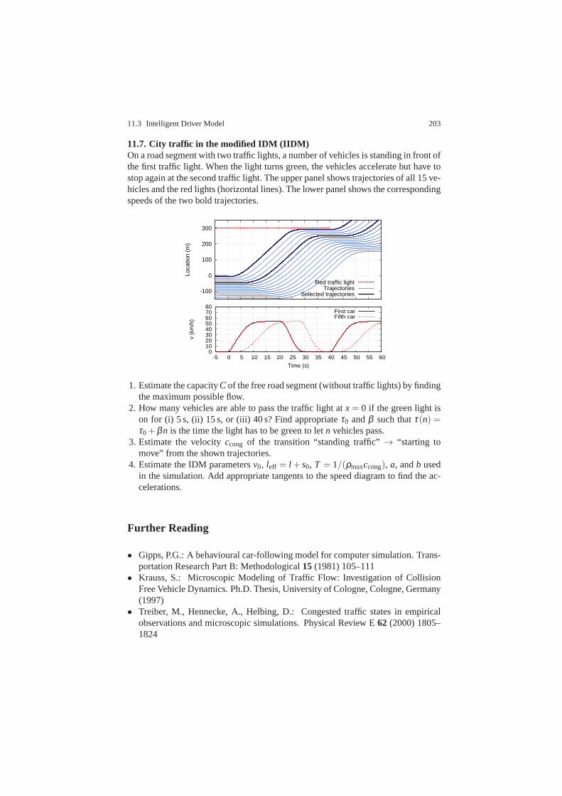
11.7. City traffic in the modified IDM (IIDM)On a road segment with two traffic lights, a number of vehiclesis standing in front ofthe first traffic light. When the light turns green, the vehicles accelerate but have tostop again at the second traffic light. The upper panel shows trajectories of all 15 ve-hicles and the red lights (horizontal lines). The lower panel shows the correspondingspeeds of the two bold trajectories.
-100
0
100
200
300
-5 0 5 10 15 20 25 30 35 40 45 50 55 60
Loca
tion
(m)
Time (s)
Red traffic lightTrajectories
Selected trajectories
0 10 20 30 40 50 60 70 80
-5 0 5 10 15 20 25 30 35 40 45 50 55 60
v (k
m/h
)
Time (s)
First carFifth car
1. Estimate the capacityC of the free road segment (without traffic lights) by findingthe maximum possible flow.
2. How many vehicles are able to pass the traffic light atx= 0 if the green light ison for (i) 5 s, (ii) 15 s, or (iii) 40 s? Find appropriateτ0 andβ such thatτ(n) =τ0+βn is the time the light has to be green to letn vehicles pass.
3. Estimate the velocityccong of the transition “standing traffic”→ “starting tomove” from the shown trajectories.
4. Estimate the IDM parametersv0, leff = l +s0, T = 1/(ρmaxccong), a, andb usedin the simulation. Add appropriate tangents to the speed diagram to find the ac-celerations.
Further Reading
• Gipps, P.G.: A behavioural car-following model for computer simulation. Trans-portation Research Part B: Methodological15 (1981) 105–111
• Krauss, S.: Microscopic Modeling of Traffic Flow: Investigation of CollisionFree Vehicle Dynamics. Ph.D. Thesis, University of Cologne, Cologne, Germany(1997)
• Treiber, M., Hennecke, A., Helbing, D.: Congested traffic states in empiricalobservations and microscopic simulations. Physical Review E 62 (2000) 1805–1824

204 11 Car-Following Models based on Driving Strategies
• Kesting, A., Treiber, M., Helbing, D.: Enhanced Intelligent Driver Model to ac-cess the impact of driving strategies on traffic capacity simulations. PhilosophicalTransactions of the Royal Society A368(2010) 4585–4605
Solutions to the Problems 459
Subproblem 3 (emergency braking).At first, we determine the initial distance suchthat a driver driving atv1 = 50km/h just manages to stop before hitting the child:
s(0) = sstop(v1) = 25.95m.
Now we consider a speedv2 = 70km/h but the same initial distances(0) = 25.95mas calculated above. At the end of the reaction time, the child is just
s(Tr) = s(0)−v2Tr = 6.50m
away from the front bumper. Now, the driver would need the additional brakingdistancesB(v2) = 23.6m for a complete stop. However, only 6.50 m are availableresulting in a difference∆s= 17.13m. With this information, the speed at collisioncan be calculated by solving∆s= (∆s)B(v) = v2/(2bmax) for v, i.e.,
vcoll =√
2bmax∆s= 16.56m/s= 59.6km/h.
Remark:This problem stems from a multiple-choice question of the theoreticalexam for a German driver’s licence. The official answer is 60 km/h.
Problems of Chapter 11
11.1 Conditions for the microscopic fundamental diagram. The plausibilitycondition (11.5) is valid for any speedvl of the leading vehicle. This also includesstanding vehicles where Eq. (11.5) becomesamic(s,0,0) = 0 for s≤ s0. This corre-sponds to the steady-state conditionve(s) = 0 for s≤ s0.
Conditions (11.1) and (11.2) are valid for any speedvl of the leader as well,including the steady-state situationvl = v or ∆v= 0. For the alternative accelerationfunctiona(s,v,∆v), this means
∂ a(s,v,0)∂s
≥ 0,∂ a(s,v,0)
∂v< 0.
Along the one-dimensional manifold of steady-state solutions{ve(s)} for s∈ [0,∞[,we have ˜a(s,ve(s),0) = 0, so the differential change d ˜a along the equilibrium curveve(s) must vanish as well:
da=∂ a(s,ve(s),0)
∂sds+
∂ a(s,ve(s),0)∂v
v′e(s)ds= 0,
hence
v′e(s) =−∂ a(s,v,0)/∂s∂ a(s,v,0)/∂v
≥ 0.

460 Solutions to the Problems
If the leading vehicle is outside the interaction range, we havev′e(s) = 0 (secondcondition of Eq. (11.2)). Finally, the condition lim
s→∞ve(s) = v0 follows directly from
the second part of condition (11.1).
11.2 Rules of thumb for the safe gap and braking distance
Subproblem 1.One mile corresponds to 1.609 km. However, the US rule does notgive explicit values for a vehicle length. Here, we assume 15ft = 4.572m. In anycase, the gaps increases linearly with the speedv, so the time gapT = s/v is inde-pendent of speed. Implementing this rule, we obtain
T =sv=
15ft10mph
=4.572m
16.09km/h=
4.572m4.469m/s
= 1.0s.
Notice that, in the final result, we rounded off generously. After all, this is a rule ofthumb and more significant digits would feign a non-existentprecision.7 Notice thatthis rule is consistent with typically observed gaps (cf. Fig. 4.8).
Subproblem 2.Here, the speedometer reading is in units of km/h, and the space gapis in units of meters. Again, the quotient, i.e., the time gapT is constant and givenby (watch out for the units)
T =sv=
12m
(
vkm/h
)
v=
12m
km/h=
0.5h1000
=1800s1000
= 1.8s.
Subproblem 3.The kinematicbraking distanceis s(v) = v2/(2b), so the cited ruleof thumb implies that the braking deceleration does not depend on speed. By solvingthe kinematic braking distance forb and inserting the rule, we obtain (again, watchout for the units)
b=v2
2s=
v2
0.02m
(
kmhv
)2
=50
3.62 m/s2 = 3.86m/s2.
For reference, comfortable decelerations are below 2m/s2 while emergency brakingdecelerations on dry roads with good grip conditions can be up to 10m/s2, about6m/s2 for wet conditions, and less than 2m/s2 for icy conditions. This means, theabove rule could lead to accidents for icy conditions but is okay, otherwise.
11.3 Reaction to vehicles merging into the lane
Reaction for the IDM.For v= v0/2, the IDM steady-state space gap reads
se(v) =s0+vT
√
1−(
vv0
)δ=
s0+v0T2
√
1−(
12
)δ.
7 There is also a more conservative variant of this rule where one should leave one car length everyfive mph corresponding to the “two-second rule”T = 2.0s.

Solutions to the Problems 461
The prevailing contribution comes from the prescribed timeheadway (fors0 = 2mand δ = 4, the other contributions only make up about 10 %). This problem as-sumes that the merging vehicle reduces the gap to the considered follower to halfthe steady-state gap,s= se/2= v0T/4, while the speed difference remain zero. Thenew IDM acceleration of the follower (witha= 1m/s2 andδ = 4) is therefore
vIDM = a
[
1−(
vv0
)δ−(
s0+vTs
)2]
(v=v0/2,s=se/2)= a
[
1−(
12
)δ−(
s0+v0T/2se/2
)2]
se(v)=se(v0/2)= −3a
[
1−(
12
)δ]
=−4516
m/s2 =−2.81m/s2.
Reaction for the simplified Gipps’ model.For this model, the steady-state gap in thecar-following regime readsse(v) = v∆ t. Again, at the time of merging, the mergingvehicle has the same speedv0/2 as the follower, and the gap is half the steady-stategap,s= (v∆ t)/2= v0∆ t/4. The new speed of the follower is restricted by the safespeedvsafe:
v(t +∆ t) = vsafe=−b∆ t +
√
b2(∆ t)2+(v0
2
)2+
bv0∆ t2
= 19.07m/s.
This results in an effective acceleration(
dvdt
)
Gipps=
v(t +∆ t)−v(t)∆ t
≈−0.93m/s2.
We conclude that the Gipps’ model describes a more relaxed driver reaction com-pared to the IDM. Notice that both the IDM and Gipps’ model would generate sig-nificantly higher decelerations for the case of slower leading vehicles (dangeroussituation).
11.4 The IDM braking strategy. A braking strategy is self-regulating if, dur-ing the braking process, thekinematically necessary deceleration bkin = v2/(2s)approaches the comfortable decelerationb. In order to show this, we calculate therate of change of the kinematic deceleration (applying the quotient and chain rulesof differentiation when necessary) and set ˙s= −v andv= −b2
kin/b= −v4/(4bs2),afterwards. This eventually gives Eq. (11.19) of the main text:
dbkin
dt=
ddt
(
v2
2s
)
=4vsv−2v2s
4s2
=v3
2s2
(
1− v2
2sb
)
=vbkin
sb
(
b−bkin)
,

462 Solutions to the Problems
11.5 Analysis of a microscopic model
Subproblem 1 (parameters).For interaction-free accelerations,vsafe> v0, sovsafe
is not relevant. Hencev0 denotes the desired speed, anda the absolute value ofthe acceleration and deceleration for the casesv< v0 andv> v0, respectively. Thesteady-state conditionss= const. andv= vl = ve = const. give
ve = min(v0,vsafe).
Without interaction,vsafe> v0, sove= v0. With interactions, the safe speed becomesrelevant and the above condition yields
ve = vsafe=−aT+√
a2T2+v2e+2a(s−s0)
which can be simplified tos= s0+veT.
Thus,s0 is the minimum gap forv = 0, andT the desired time gap. The modelproduces a deceleration−a not only if v > v0 (driving too fast in free traffic) butalso if v > vsafe (driving too fast in congested situations). Furthermore, the modelis symmetrical with respect to accelerations and decelerations. Obviously, it is notaccident free.
Subproblem 2 (steady-state speed).We have already derived the steady-state con-dition
ve(s) = min
(
v0,s−s0
T
)
.
Macroscopically, this corresponds to the triangular fundamental diagram
Qe(ρ) = min
(
v0ρ ,1−ρ leff
T
)
where leff = 1/ρmax = l + s0. The capacity per lane is given byQmax = (T +leff/v0)
−1 = 1800vehicles/h at a densityρC = 1/(leff + v0T) = 25/km. For fur-ther properties of the triangular fundamental diagram, seeSection 8.5.
Subproblem 3.The acceleration and braking distances to accelerate from 0to20m/s or to brake from 20m/s to 0, respectively, are the same:
sa = sb =v2
0
2a= 200m.
At a minimum gap of 3 m and the locationxstop= 603m of the stopping line ofthe traffic light, the acceleration takes place fromx = 0 to x1 = 200m, and thedeceleration fromx2 = 400m tox3 = 600m. The duration of the acceleration anddeceleration phases isv0/a = 20s while the time to cruise the remaining stretchof 200 m atv0 amounts to 10 s. This completes the information to mathematicallydescribe the trajectory:

Solutions to the Problems 463
x(t) =
12at2 t ≤ t1 = 20s,x1+v0(t − t1) t1 < t ≤ t2 = 30s,x2+v0(t − t2)− 1
2a(t − t2)2 t2 < t ≤ t3 = 50s,
wheret1 = 20s,t2 = 30s andt3 = 50s.
11.6 Heterogeneous traffic.The simultaneous effects of heterogeneous traffic andseveral lanes with lane-changing and overtaking possibilities results in a curved freepart of the fundamental diagram even for models that would display a triangularfundamental diagram for identical vehicles and drivers (asthe Improved IntelligentDriver Model, IIDM). This can be seen as follows: For heterogeneous traffic, eachvehicle-driver class has a different fundamental diagram.Particularly, the densityρC
at capacity is different for each class, so a simple weightedaverage of the individualfundamental diagrams would result in a curved free part and arounded peak. How-ever, without lane-changing and overtaking possibilities, all vehicles would queueup behind the vehicles of the slowest class resulting in a straight free part of the fun-damental diagram with the gradient representing the lowestfree speed.8 So, bothheterogeneity and overtaking possibilities are necessaryto produce a curved freepart of the fundamental diagram.
11.7 City traffic in the improved IDM
-100
0
100
200
300
-5 0 5 10 15 20 25 30 35 40 45 50 55 60
Loca
tion
(m)
Time (s)
Red traffic lightTrajectories
Selected trajectories
0 10 20 30 40 50 60 70 80
-5 0 5 10 15 20 25 30 35 40 45 50 55 60
v (k
m/h
)
Time (s)
First carFifth car
72 km/h=20 m/s
1. For realistic circumstances, the maximum possible flow isgiven by thedynamiccapacity, i.e., the outflow from moving downstream congestion fronts. In ourcase, the “congestion” is formed by the queue of standing vehicles behind a trafficlight. Counting the trajectories (horizontal double-arrow in the upper diagram)yields
C= Qmax≈9vehicles
20s= 1620vehicles/h.
8 Even when obstructed, drivers can choose their preferred gap (in contrast to the desired speed), sothe congested branch of the fundamental diagram is curved evenwithout overtaking possibilities.
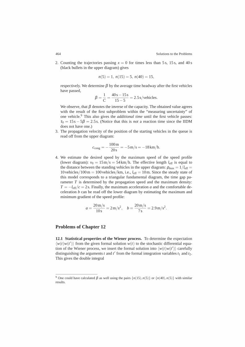
464 Solutions to the Problems
2. Counting the trajectories passingx = 0 for times less than 5 s, 15 s, and 40 s(black bullets in the upper diagram) gives
n(5) = 1, n(15) = 5, n(40) = 15,
respectively. We determineβ by the average time headway after the first vehicleshave passed,
β =1C
=40s−15s
15−5= 2.5s/vehicles.
We observe, thatβ denotes the inverse of the capacity. The obtained value agreeswith the result of the first subproblem within the “measuringuncertainty” ofone vehicle.9 This also gives theadditional timeuntil the first vehicle passes:τ0 = 15s− 5β = 2.5s. (Notice that this isnot a reaction time since the IIDMdoes not have one.)
3. The propagation velocity of the position of the starting vehicles in the queue isread off from the upper diagram:
ccong=−100m20s
=−5m/s=−18km/h.
4. We estimate the desired speed by the maximum speed of the speed profile(lower diagram):v0 = 15m/s= 54km/h. The effective lengthleff is equal tothe distance between the standing vehicles in the upper diagram:ρmax= 1/leff =10vehicles/100m= 100vehicles/km, i.e.,leff = 10m. Since the steady state ofthis model corresponds to a triangular fundamental diagram, the time gap pa-rameterT is determined by the propagation speed and the maximum density:T =−leff/c= 2s. Finally, the maximum accelerationa and the comfortable de-celerationb can be read off the lower diagram by estimating the maximum andminimum gradient of the speed profile:
a=20m/s
10s= 2m/s2, b=
20m/s7s
= 2.9m/s2.
Problems of Chapter 12
12.1 Statistical properties of the Wiener process.To determine the expectation〈w(t)w(t ′)〉 from the given formal solutionw(t) to the stochastic differential equa-tion of the Wiener process, we insert the formal solution into 〈w(t)w(t ′)〉 carefullydistinguishing the argumentst andt ′ from the formal integration variablest1 andt2.This gives the double integral
9 One could have calculatedβ as well using the pairs{n(15),n(5)} or {n(40),n(5)} with similarresults.