chapter 1 petrophysical rock propertiesof the petrophysical properties porosity, permeability,...

Chapter 1 Petrophysical Rock Properties

1.1 Introduction

The principal goal of reservoir characterization is to construct three-dimensional images of petrophysical properties. The purpose of this chapter is to review basic definitions and laboratory measurements of the petrophysical properties porosity, permeability, relative per-meability, capillarity, and saturation. Pore-size distribution is pre-sented as the common link between these properties.

1.2 Porosity

Porosity is an important rock property because it is a measure of the potential storage volume for hydrocarbons. Porosity in carbonate reservoirs ranges from 1 to 35% and, in the United States, averages 10% in dolomite reservoirs and 12% in limestone reservoirs (Schmoker et al. 1985).

Porosity is defined as pore volume divided by bulk volume.

eBulk volum volumeMineral-eBulk volum

eBulk volum volumePore

==Porosity (1)

Fractional porosity is used in engineering calculations. Geologists,

however, most commonly refer to porosity as a percentage (porosity x 100). The term “effective porosity” or “connected” pore space is com-monly used to denote porosity that is most available for fluid flow. How-ever, at some scale all pore space is connected. The basic question is how the pore space is connected, which will be the principal focus of this book.

2 Chapter 1 Petrophysical Rock Properties

Porosity is a scalar quantity because it is a function of the bulk volume used to define the sample size. Therefore, whereas the porosity of Carls-bad Caverns is 100% if the caverns are taken as the bulk volume, the po-rosity of the formation including Carlsbad Caverns is much less and de-pends upon how much of the surrounding formation is included as bulk volume. Calculating the porosity of caves using a “boundary volume” for bulk volume results in porosity values for the caves in the 0.5% range (Sasowsky, personal communication). Thus, porosity is always a number, and the value is a function of the bulk volume chosen. The term “poros-ity” is often misused in place of “pore space,” which is the proper term for describing voids in a rock. Porosity is a measurement and cannot be seen, whereas what is observed is pore space, or pores. The misuse of these terms often leads to confusion, especially when discussing the “origin of porosity,” which is the origin of the pore space or the history of changes in porosity.

Porosity is determined by visual methods and laboratory measurements. Visual methods of measuring total porosity are estimates at best because the amount of porosity visible depends on the method of observation: the higher the magnification, the more pore space is visible. Porosity is commonly estimated by visual inspection of core slabs using a low-power microscope. The Archie classification (Archie 1952) provides a method of combining textural criteria and visible porosity to determine total porosity. Visible porosity in thin section can be measured by point counting the visible pores or by using image analysis software to calculate pore space. The thin section is taken as the bulk volume. Visual estimates can be very inaccurate unless calibrated against point-counted values. Commonly, visual estimates of porosity are twice as high as point-counted values. Laboratory porosity values are normally higher than visual estimates because very small pore space cannot be seen with visual observational techniques. When all the pore space is large, such as in grainstones, however, point-counted values are comparable with measured values.

Measurement of porosity of rock samples in the laboratory requires knowing the bulk volume of the rock and either its pore volume or the volume of the matrix material (mineral volume). Bulk volume is usually measured by volumetric displacement of a strongly nonwetting fluid, such as mercury, or by direct measurement of a regularly shaped sample. Pore volume can be obtained in a number of ways. If the mineralogy is known, mineral volume can be calculated from grain density and the sample weight; pore volume is bulk volume minus mineral volume. The most accurate method of measuring porosity is the helium expansion method. A dried sample is placed in a chamber of known volume and the pressure is measured with and without the sample, keeping the volume of gas constant. The

1.2 Porosity 3

difference in pressure indicates the pore volume. A grain density is reported for each sample, and the accuracy of the porosity value can be judged by how close the density is to a known mineral density. If the density values reported are less than 2.8 for dolostone samples, for example, the porosity values are probably too low. The injection of mercury under very high pressure (the porosimeter) is also used to measure porosity. However, this is a destructive method and is normally used only under special circumstances. Summations-of-fluids is an old technique that attempts to use the fluids removed from the core to measure pore volume. It is very inaccurate and no longer in use. However, old porosity measurements may have been made using this inaccurate technique.

The complete removal of all fluids is critical for accurate measurements of porosity. Any fluid that is not removed will be included as part of the mineral volume, resulting in porosity values being too low. An example of incomplete removal of all fluids is taken from the Seminole San Andres field (Lucia et al. 1995). The whole-core analysis porosity values were suspected of being too low, and 11 whole-core samples were reanalyzed by drilling three 1-in plugs from each sample and cleaning the plugs in an industry laboratory in which special care was taken to remove all water and oil. The average porosity of all but one of the samples was higher than the whole-core porosity by an average of 2 porosity units (Fig. 1).

Fig. 1.1. Plot of whole-core porosity values versus porosity values of plug samples taken from the whole-core samples and recleaned. Whole-core porosity is too small by 0 – 4 porosity percent

Subjecting samples that contain gypsum to high temperatures in laboratory procedures results in dehydrating gypsum to the hemihydrate form Bassanite (see Eq. 2) and creating pore space and free water, both of which produce large errors in the porosity measurements (Table 1). Pore space is created because Bassanite (density 2.70) has a smaller molar volume than


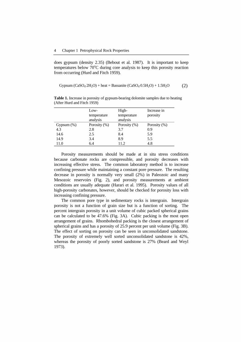
does gypsum (density 2.35) (Bebout et al. 1987). It is important to keep temperatures below 70oC during core analysis to keep this porosity reaction from occurring (Hurd and Fitch 1959).

Gypsum (CaSO4⋅2H2O) + heat = Bassanite (CaSO4⋅0.5H2O) + 1.5H2O (2)

Table 1. Increase in porosity of gypsum-bearing dolomite samples due to heating (After Hurd and Fitch 1959)

Low-temperature analysis

High-temperature analysis

Increase in porosity

Gypsum (%) Porosity (%) Porosity (%) Porosity (%) 4.3 2.8 3.7 0.9 14.6 2.5 8.4 5.9 14.9 3.4 8.9 5.5 11.0 6.4 11.2 4.8

Porosity measurements should be made at in situ stress conditions

because carbonate rocks are compressible, and porosity decreases with increasing effective stress. The common laboratory method is to increase confining pressure while maintaining a constant pore pressure. The resulting decrease in porosity is normally very small (2%) in Paleozoic and many Mesozoic reservoirs (Fig. 2), and porosity measurements at ambient conditions are usually adequate (Harari et al. 1995). Porosity values of all high-porosity carbonates, however, should be checked for porosity loss with increasing confining pressure.

The common pore type in sedimentary rocks is intergrain. Intergrain porosity is not a function of grain size but is a function of sorting. The percent intergrain porosity in a unit volume of cubic packed spherical grains can be calculated to be 47.6% (Fig. 3A). Cubic packing is the most open arrangement of grains. Rhombohedral packing is the closest arrangement of spherical grains and has a porosity of 25.9 percent per unit volume (Fig. 3B). The effect of sorting on porosity can be seen in unconsolidated sandstone. The porosity of extremely well sorted unconsolidated sandstone is 42%, whereas the porosity of poorly sorted sandstone is 27% (Beard and Weyl 1973).

1.2 Porosity 5

Fig. 1.2. Effect of confining pressure on porosity in Paleozoic and Jurassic carbonate reservoirs. Porosity loss is defined as confined porosity/unconfined porosity

Fig. 1.3. Comparison of porosity in (A) cubic packed spheres and (B) rhombohedral-packed spheres. The porosity is a function of packing, and pore size is controlled by the size and packing of spheres

In carbonate sediment the shape of the grains and the presence of intragrain porosity as well as sorting have a large effect on porosity. The presence of pore space within shells and peloids that make up the grains of carbonate sediments increases the porosity over what would be expected from intergrain porosity alone (Dunham 1962). The effect of sorting on porosity is opposite from that found in siliciclastics. The porosity of modern


ooid grainstones averages 45% but porosity increases to 70 percent as sorting decreases (Enos and Sawatski 1981). This increase is largely related to the needle shape of the mud-sized aragonite crystal. As a result, there is no simple relationship among porosity, grain size, and sorting in carbonate rocks.

Although there is no simple relation between porosity and fabric, it is apparent by inspection that intergrain pore size decreases with smaller grain size and with closer grain packing. Porosity also decreases with closer packing, resulting in intergain pore size being related to grain size, sorting, and intergrain porosity. The size and volume of intragrain pore space are related to the type of sediment and its post-depositional history.

1.3 Permeability

Permeability is important because it is a rock property that relates to the rate at which hydrocarbons can be recovered. Values range considerably from less than 0.01 millidarcy (md) to well over 1 darcy. A permeability of 0.1 md is generally considered minimum for oil production. Highly productive reservoirs commonly have permeability values in the Darcy range.

Permeability is expressed by Darcy’s Law:

Darcy’s Law: ⎟⎠⎞

⎜⎝⎛ Δ⎟⎟⎠

⎞⎜⎜⎝

⎛=

LPkAQ

μ,

(3)

where Q is rate of flow, k is permeability, μ is fluid viscosity, (ΔP)/L is the potential drop across a horizontal sample, and A is the cross-sectional area of the sample. Permeability is a rock property, viscosity is a fluid property, and ΔP/L is a measure of flow potential.

Permeability is measured in the laboratory by encasing a sample of known length and diameter in an air-tight sleeve (the Hasseler Sleeve) in a horizontal position. A fluid of known viscosity is injected into a sample of known length and diameter while mounted in a horizontal position. The samples are either lengths of whole core, typically 6 inches long, or 1-in plugs drilled from the cores. The pressure drop across the sample and the flow rate are measured and permeability is calculated using the Darcy equation (Fig. 4). Normally, either air or brine is used as a fluid and, when high rates of flow can be maintained, the results are comparable. At low rates, air permeability will be higher than brine permeability. This is because gas does not adhere to the pore walls as liquid does, and the slippage of gases along the pore walls gives rise to an apparent dependence of permeability on

1.3 Permeability 7

pressure. This is called the Klinkenberg effect, and it is especially important in low-permeability rocks.

Fig. 1.4. Method of measuring permeability of a core plug in the laboratory. Sam-ples are oriented horizontally to eliminate gravity effects; see text for explanation

Permeability can also be measured using a device called the miniairpermeameter (Hurst and Goggin 1995). This device is designed for use on flow surfaces such as outcrops or core slabs, and numerous permeability values can be obtained quickly and economically. This method, however, is not as accurate as the Hasseler Sleeve method. The equipment consists of a pressure tank, a pressure gauge, and a length of plastic hose with a special nozzle or probe designed to fit snugly against the rock sample. The gas pressure and the flow rate into the rock sample are used to calculate permeability.

Measurements should be made when the samples are under some confining pressure, preferably a confining pressure equivalent to in situ reservoir conditions. This is particularly important when the samples contain small fractures and stylolites because in unconfined conditions these features tend to be flow channels that result in unreasonably high permeability values.

Permeability is a vector and scalar quantity. Horizontal permeability varies in different directions, and vertical permeability is commonly less than horizontal permeability. Therefore, permeability is often represented as a vector in the x, y, and z directions. Core analysis reports give three permeability values when whole-core samples are used, two horizontal and one vertical, and a single horizontal value when core plugs are used. The two horizontal measurements are taken at 90 degrees from each other and are


commonly represented as maximum permeability and permeability 90 degrees from maximum.

Permeability depends upon the volume of the sample as well as the orientation. Darcy’s Law shows permeability as a function of the cross-sectional area of the sample and pressure drop along a fixed length. In carbonate reservoirs permeability varies depending upon the size of the sample. An extreme example of the sampling problem is illustrated by a core sample with a large vug from a Silurian carbonate buildup (Fig. 5). The permeability of this sample is most likely very large because of the large touching vug, but the core analysis reports permeability at <0.1 md. This value is based on a 1-in plug, which was used because it would be very difficult to measure the permeability of the whole-core sample. Therefore, it is important to know how the formation was sampled before using the laboratory results. As a rule, never use core data from a carbonate reservoir unless you have seen the core and observed how the core was sampled.

Fig. 1.5. Core sample of a large vug from a Silurian reef, Michigan. The measured permeability from a core plug taken from this sample is <0.1md, which is an obvious understatement of the permeability of this sample

A measure of permeability can be obtained from production tests using pressure buildup analyses. The pressure in the well is drawn down by production, the well is shut in, and the rate of pressure increase is measured.

1.3 Permeability 9

The rate of pressure increase is a function of the effective permeability of the reservoir. The effective, average permeability of the interval tested is calculated using the following equation:

Slope (psi/log cycle) = 162.6(qμBBo/kh), (4)

where q is the flow rate in stock-tank-barrels/day, μ = viscosity in centipoises, Bo is reservoir-barrels/stock-tank-barrels, k is permeability in millidarcys, and h is the net reservoir interval in feet.

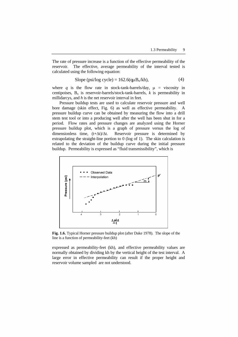
Pressure buildup tests are used to calculate reservoir pressure and well bore damage (skin effect, Fig. 6) as well as effective permeability. A pressure buildup curve can be obtained by measuring the flow into a drill stem test tool or into a producing well after the well has been shut in for a period. Flow rates and pressure changes are analyzed using the Horner pressure buildup plot, which is a graph of pressure versus the log of dimensionless time, (t+Δt)/Δt. Reservoir pressure is determined by extrapolating the straight-line portion to 0 (log of 1). The skin calculation is related to the deviation of the buildup curve during the initial pressure buildup. Permeability is expressed as “fluid transmissibility”, which is

Fig. 1.6. Typical Horner pressure buildup plot (after Dake 1978). The slope of the line is a function of permeability-feet (kh)

expressed as permeability-feet (kh), and effective permeability values are normally obtained by dividing kh by the vertical height of the test interval. A large error in effective permeability can result if the proper height and reservoir volume sampled are not understood.


1.4 Pore Size and Fluid Saturation

Pore-size is the common factor between permeability and hydrocarbon saturation. Permeability models have historically described pore space in terms of the radius of a series of capillary tubes. The number of capillary tubes has been equated to porosity so that permeability is a function of po-rosity and pore-radius squared (Eq. 5 from Amyx et al. 1960, p. 97). Koz-eny (1927) substituted surface area of the pore space for pore radius and developed the well-known Kozeny equation relating permeability to poros-ity, surface-area squared, and the Kozeny constant (Eq. 6).

k = πr2/32, or k = φr2/8 (5)

k = φ/kzSp2 (6)

It is common practice to estimate permeability using simple porosity-permeability transforms developed from core data. However, porosity-permeability cross plots for carbonate reservoirs commonly show large variability (Fig. 7), demonstrating that factors other than porosity are important in modeling permeability. These equations illustrate that the size and distribution of pore space, or pore-size distribution, is important along with porosity in estimating permeability. In general it can be concluded that there is no relationship between porosity and permeability in carbonate rocks unless pore-size distribution is included.

A measure of pore-size can be obtained from mercury capillary pressure curves, which are acquired by injecting mercury (nonwetting phase) into a sample containing air (wetting phase). Mercury is injected at increments of increasing pressure and a plot of injection pressure against the volume of mercury injected (Hg saturation) is made (Fig. 8). The Hg saturation can be plotted as a percent of pore volume or bulk volume. This curve is referred to as the drainage curve. As the injection pressure is reduced, wetting fluid (air or water) will flow into the pore space and the nonwetting fluid will be expelled. This process is called imbibition, and a plot of pressure and saturation during the reduction of injection pressure is referred to as the imbibition curve (Fig. 8).

The pore size obtained by this method is referred to as the pore-throat size. Pore-throat size is defined as the pore size that connects the larger pores. It is based on the concept that interparticle pore space can be visualized as rooms with connecting doors. The doors are the pore-throats that connect the larger pores, or rooms.

Hg saturation is dependent on (1) the interfacial tension between mercury and water, (2) the adhesive forces between the fluids and the minerals that

1.4 Pore Size and Fluid Saturation 11

Fig. 1.7. Plot of porosity and permeability for carbonate rocks, illustrating that there is no relationship between porosity and permeability in carbonate rocks without in-cluding pore-size distribution

Fig. 1.8. Typical capillary pressure curves showing drainage and imbibition curves. Data for the drainage curve are obtained by increasing pressure, whereas data for the imbibition curve are obtained by reducing pressure


make up the pore walls, (3) the pressure differential between the mercury and water phases (capillary pressure), and (4) pore-throat size. Pore-throat size is calculated using the following equation:

rc = 0.145(2σcosθ/Pc), (7)

where rc is the radius of the pore throat in microns, σ is the interfacial tension in dynes/cm, Pc is the capillary pressure in psia (not dynes/cm2), and 0.145 is a conversion factor to microns Interfacial tension results from the attraction of molecules in a liquid to

each other. It can be defined in terms of the pressure across the fluid boundary and the radius of curvature of that boundary, as shown in Eq. (8).

2σ = (P1-P2) rl , (8)

where P1-P2 is the pressure differential across the meniscus (capillary pressure), σ is surface tension, and rl is the radius of curvature of the liquid.

Equation (8) can be derived by considering the hemispherical bottom part of a drip of water coming out of a small faucet just before it drops. The molecules within the drip attract each other equally, but the molecules on the surface are attracted toward the center of the drip and to the other molecules on the surface, creating a net inward force (Fig. 9).

If F↓ = total downward force pulling on drip, then:

F↓ = πrl2 (P1-P2), (9)

where πrl

2 = cross-sectional area of drip and (P1-P2) = difference between the pressure inside the drip (water pressure) and pressure outside the drip (atmospheric pressure).

If F↑ = upward cohesive forces holding drip together, then F↑ = 2π rl σ ,

F↑ = 2π rl σ, (10)

where rl = radius of curvature of liquid, 2π rl = circumference of drip and σ = surface tension.


At equilibrium, F↑ = F↓ 2π rl σ = πrl

2 (P1-P2) or:

2σ/ rl = (P1-P2). (11)

Fig. 1.9. Cohesive forces and the definition of surface tension

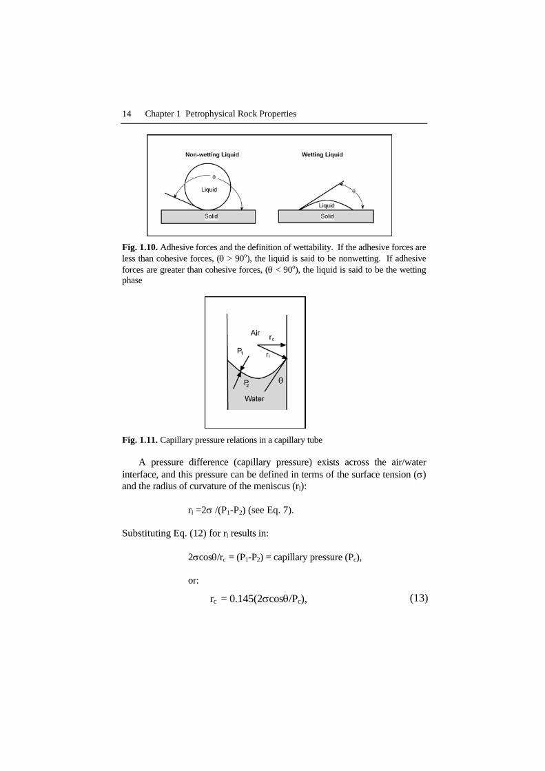
Whereas cohesive forces hold the liquid together, adhesive forces between solid and liquid tend to spread the liquid out. When a fluid encounters a solid surface, it tends either to spread over that surface or to form a ball on the surface, and the angle between the solid and liquid meniscus is a measure of the adhesive force. The contact angle between the fluid and the surface will be less than 90o for fluids that spread over the surface and greater than 90o for fluids that tend to form a ball. If the contact angle is less than 90o, the fluid is said to be wetting and if the angle is greater than 90o, nonwetting (Fig. 10).

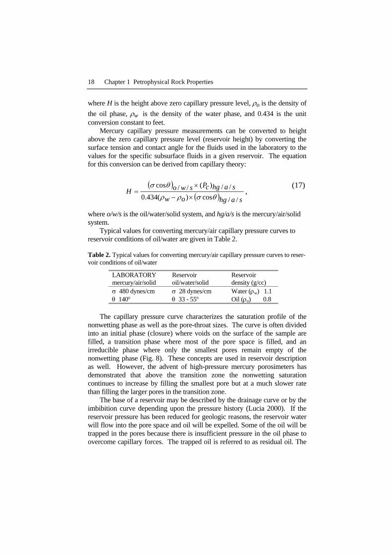
The adhesive forces between a solid and water are greater than those between a solid and air in a water/air/solid capillary system and cause water to rise in a capillary tube (Fig. 11). The adhesive force is equal to cos θ, and is equal to the radius of the capillary tube divided by the radius-of-curvature of the liquid meniscus (Eq 12):

cos θ = rc/rl , or rl = rc/cos θ, (12)

where rl is the radius of the liquid meniscus, rc is the radius of the capillary tube, and cos θ is the adhesive force (solid/liquid).


Fig. 1.10. Adhesive forces and the definition of wettability. If the adhesive forces are less than cohesive forces, (θ > 90o), the liquid is said to be nonwetting. If adhesive forces are greater than cohesive forces, (θ < 90o), the liquid is said to be the wetting phase

Fig. 1.11. Capillary pressure relations in a capillary tube

A pressure difference (capillary pressure) exists across the air/water interface, and this pressure can be defined in terms of the surface tension (σ) and the radius of curvature of the meniscus (rl):

rl =2σ /(P1-P2) (see Eq. 7).

Substituting Eq. (12) for rl results in: 2σcosθ/rc = (P1-P2) = capillary pressure (Pc), or:

rc = 0.145(2σcosθ/Pc), (13)


where rc is the radius of the pore throat in microns, σ is the interfacial tension in dynes/cm, Pc is the capillary pressure in psia (not dynes/cm2), and 0.145 is a conversion factor to microns Pore-throat sizes are calculated for each point on the capillary pressure

curve and presented a frequency or cumulative frequency plot as shown in Fig. 12. These plots characterize the statistical distribution of pore-throat sizes in the sample but do not characterize their spatial distribution. Also, these curves do not characterize all the pore sizes that are in the sample, only the pore-throat size. However, techniques have been developed to obtain a measure of larger pore sizes as well as pore-throat sizes from mercury injection. Pore-size distribution as used in this book is defined as the spatial distribution of all the pore sizes in the rock, which includes pore-throat sizes.

In order to relate pore-throat size, determined from mercury capillary pressure data, to permeability and porosity as discussed above, a normalizing pore size must be chosen (Swanson 1981). The pore-throat size at a mercury saturation of 35% has been determined to be most useful (Kolodizie 1980; Pittman 1992). Generic equations relating porosity, permeability, and pore-throat size at various mercury saturations for siliciclastics have been published by Pittman (1992). A plot using 35% mercury saturation to calculate pore-throat size (Fig. 13) demonstrates that pore-throat size has a larger effect on permeability than does porosity. Because these equations are derived for siliciclastic rocks, the porosity is restricted to intergrain porosity and not necessarily to total porosity.

Fig. 1.12. A frequency diagram of pore-throat sizes (A) is calculated from the mer-cury capillary pressure curve (B)


Fig. 1.13. Plot of porosity, permeability, and pore-throat size for siliciclastic rocks using 35% mercury saturation to calculate pore-throat size from mercury capillary pressure curves (Pittman 1992)

Log(r35) = 0.255 + 0.565Log(k) - 0.523Log(φ)

where r35 = pore-throat radius at 35% mercury saturation in microns,

k = permeability in millidarcys, and φ = interparticle porosity as a fraction. A similar equation has been published by Kolodizie (1980) and is

presented here. It is referred to as the Winland equation and is used more commonly in the petroleum industry than is Pittman’s equation.

701.1

35470.15.49 rk φ=

Hydrocarbon saturation in a reservoir is related to pore size as well as

capillary pressure and capillary forces. For oil to accumulate in a hydrocarbon trap and form a reservoir, the surface tension between water and oil must be exceeded. This means that the pressure in the oil phase must be higher than the pressure in the water phase. If the pressure in the oil is only slightly greater than that in the water phase, the radius of curvature will be large and the oil will be able to enter only large pores. As the pressure in the oil phase increases, the radius of curvature decreases and oil can enter smaller pores (Fig. 14).


Fig. 1.14. Diagram showing smaller pores being filled with a non-wetting fluid (oil) displacing a wetting fluid (water) as capillary pressure increases linearly with reser-voir height. Pore size is determined by grain size and sorting. (A) Only the largest pores contain oil at the base of the reservoir. (B) Smaller pores are filled with oil as capillary pressure and reservoir height increase. (C) Smallest pores are filled with oil toward the top of the reservoir

In nature, the pressure differential (capillary pressure) is produced by the difference in density between water and oil; the buoyancy effect. At the zero capillary pressure level (zcp), the reservoir pressure is equal to pressure in the water phase (depth times water density). Above the zcp level the pressure in the water phase will be reduced by the height above the zcp times water density, and the pressure in the oil phase will be reduced by the height above the zcp times oil density.

Pressure in water phase wHzcpPwP ρ−= (14)

Pressure in oil phase ozcpo HPP ρ−= (15)

At any height in an oil column, the pressure difference between the oil phase and the water phase (capillary pressure) is the difference between the specific gravity of the two fluids multiplied by the height of the oil column:

( )owHwPoP ρρ −=− 434.0 , (16)


where H is the height above zero capillary pressure level, ρo is the density of the oil phase, ρw is the density of the water phase, and 0.434 is the unit conversion constant to feet.

Mercury capillary pressure measurements can be converted to height above the zero capillary pressure level (reservoir height) by converting the surface tension and contact angle for the fluids used in the laboratory to the values for the specific subsurface fluids in a given reservoir. The equation for this conversion can be derived from capillary theory:

( )( ) sahgow

sahgcPswoH//cos)(434.0

//)(//cos

θσρρ

θσ

×−

×= ,

(17)

where o/w/s is the oil/water/solid system, and hg/a/s is the mercury/air/solid system.

Typical values for converting mercury/air capillary pressure curves to reservoir conditions of oil/water are given in Table 2.

Table 2. Typical values for converting mercury/air capillary pressure curves to reser-voir conditions of oil/water

LABORATORY mercury/air/solid

Reservoir oil/water/solid

Reservoir density (g/cc)

σ 480 dynes/cm σ 28 dynes/cm Water (ρw) 1.1 θ 140° θ 33 - 55° Oil (ρo) 0.8

The capillary pressure curve characterizes the saturation profile of the

nonwetting phase as well as the pore-throat sizes. The curve is often divided into an initial phase (closure) where voids on the surface of the sample are filled, a transition phase where most of the pore space is filled, and an irreducible phase where only the smallest pores remain empty of the nonwetting phase (Fig. 8). These concepts are used in reservoir description as well. However, the advent of high-pressure mercury porosimeters has demonstrated that above the transition zone the nonwetting saturation continues to increase by filling the smallest pore but at a much slower rate than filling the larger pores in the transition zone.

The base of a reservoir may be described by the drainage curve or by the imbibition curve depending upon the pressure history (Lucia 2000). If the reservoir pressure has been reduced for geologic reasons, the reservoir water will flow into the pore space and oil will be expelled. Some of the oil will be trapped in the pores because there is insufficient pressure in the oil phase to overcome capillary forces. The trapped oil is referred to as residual oil. The


reservoir will be in imbibition mode, and the imbibition curve must be used to describe the fluid distribution at the bottom of the reservoir. The drainage transition zone is replaced by a thinner imbibition transition zone and a residual oil zone.

The difference in density between water and hydrocarbons, the buoyancy force, produces pressures in hydrocarbon columns that exceed pressures in the water column. The pressure gradient in reservoirs can be used to determine the distance above the zcp level. Multiple reservoir pressures can be obtained from the repeat formation tester, a wireline formation tester capable of multiple settings downhole (Smolen and Litsey 1977). It can retrieve several fluid samples per trip, but its primary advantage is its multiple-level pressure-measuring capability. This tool allows a number of pressures to be taken from selected intervals, thus providing data to determine reservoir gradients. This data can be used to define zcp levels and define reservoir compartments (Fig. 15).

Fig. 1.15. Diagram illustrating the use of pressure gradients to define reservoir com-partments and water levels. (A) Depth plot of pressure from wells 1 and 2 shown in (B). Intersections of depth plots with the regional fluid-pressure gradient are at depths d1 and d2, suggesting separate reservoirs with different water-oil contacts. (B) Cross section showing well locations, sampling depths, and sealing fault dividing the hydrocarbon accumulation into two reservoirs

The pressure in the water phase depends upon the degree to which the fluid column is connected to the Earth’s surface. In an open system, the fluid pressure is equal to depth times the density of the fluid and is called hydrostatic (Fig. 16). The hydrostatic pressure gradient is about 0.434 psi/ft; overburden pressure equals the weight of the overburden sediment and has a gradient of about 1 psi/ft. Deviations from hydrostatic pressure, abnormal pressures, occur when the formation fluid is confined and cannot equilibrate with surface pressure. Overpressuring is the most common abnormal pressure and is produced by (1) compaction during rapid burial, (2) tectonic


compression, and (3) hydrocarbon generation and migration (Osborne and Swarbrick 1997). In extreme cases, fluid pressures can equal and even exceed overburden pressures. Uncommonly, pressures can be lower than hydrostatic. Underpressure is often related to erosional unloading that results in an increase in pore volume due to the elastic rebound of the sediment as the overburden is reduced (Bachu and Underschultz 1995).

Fig. 1.16. Diagram illustrating overburden, normal hydrostatic, and abnormal over- and underpressure regimes. (After Dake 1978)

1.5 Relative Permeability

Oil, water, and gas are found in hydrocarbon reservoirs in varying propor-tions. Permeability measurements, however, are typically done using a single fluid, commonly air or water, and the permeability values must be corrected for the varying saturations of water, oil, and gas that occur in the reservoir. The correction is necessary because when a non-wetting fluid, such as oil, enters a water-wet pore system, the oil fills the centers of the largest, well connected pores whereas the water is found lining the pore walls and filling the smallest pores. This fluid distribution reduces the pore space available for flow of either water or oil. When water is injected or imbibed into the water-wet pore system, oil is trapped in pores with the

1.5 Relative Permeability 21

smallest portals due to capillary forces. This oil is referred to as residual oil to water flooding (Fig. 17).

Fig. 1.17. Diagram of oil and water distribution in a water-wet rock under three con-ditions: (A) 100% water saturation, (B) injection of a nonwetting fluid (oil), and (C) injection of a wetting fluid (water)

Relative permeability is simply the permeability measured at a specific fluid saturation expressed as a fraction of the total or absolute permeability. Absolute permeability is the permeability of a rock that is 100% saturated with a single fluid. In a water-wet rock only water can totally saturate the pore system, and brine permeability is normally taken as the absolute permeability. However, hydrocarbon permeability at residual water saturation is often used as absolute permeability in reservoir engineering studies. Effective permeability is the permeability of one fluid in the presence of another fluid measured at a specific saturation state. Effective permeability is always lower than the absolute permeability and will change as the saturation changes. Thus, if a rock 100% saturated with brine has a permeability of 50 md whereas the brine permeability in the presence of 50% oil saturation is 10 md, the relative permeability of brine at 50% oil saturation is said to be 0.2. Graphs of relative permeability versus saturation (Fig. 18) are very important because they can be used to predict changes in production rates with changes in water saturation. They are fundamental in fluid flow


simulation, and changing the relative permeability characteristics has a major effect on the resulting performance prediction.

Fig. 1.18. Typical relative permeability plot where absolute permeability is taken as oil permeability at lowest water saturation. Kro is the relative permeability to oil and Krw is the relative permeability to water

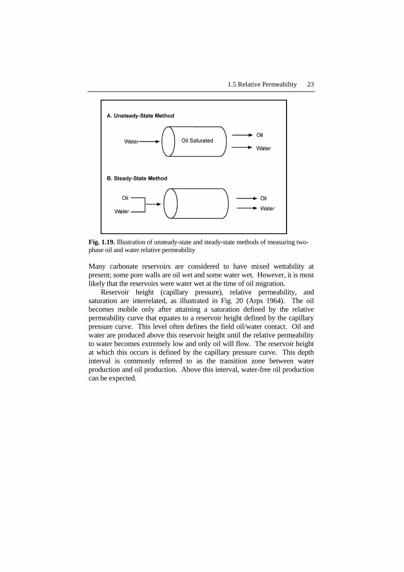
There are two methods for measuring permeability at various saturation states to obtain relative permeability, steady state and unsteady state (Fig. 19). The steady-state method is the most accurate method, but it is time consuming and expensive because it involves injecting both oil and water simultaneously until the output rates match the input rates. The unsteady-state method is less accurate but faster because it involves saturating the core with oil and flooding with water. The relationships between relative permeability and saturation obtained by these two methods are commonly very different. A third method that is rapid and less expensive is to measure effective permeabilities at irreducible water and residual oil. This is called the end point method, and it assumes that a reasonable estimate of the curvature can be made.

A significant problem in measuring relative permeability in the laboratory is restoring samples to reservoir conditions. Pore surfaces, especially in carbonate rocks, are reactive to changes in fluids, and these reactions can alter the wettability state. Elaborate methods have been devised to preserve the original wettability state of core material, and the accuracy of any relative permeability data is dependent on the success of these methods.

1.5 Relative Permeability 23

Fig. 1.19. Illustration of unsteady-state and steady-state methods of measuring two-phase oil and water relative permeability

Many carbonate reservoirs are considered to have mixed wettability at present; some pore walls are oil wet and some water wet. However, it is most likely that the reservoirs were water wet at the time of oil migration.

Reservoir height (capillary pressure), relative permeability, and saturation are interrelated, as illustrated in Fig. 20 (Arps 1964). The oil becomes mobile only after attaining a saturation defined by the relative permeability curve that equates to a reservoir height defined by the capillary pressure curve. This level often defines the field oil/water contact. Oil and water are produced above this reservoir height until the relative permeability to water becomes extremely low and only oil will flow. The reservoir height at which this occurs is defined by the capillary pressure curve. This depth interval is commonly referred to as the transition zone between water production and oil production. Above this interval, water-free oil production can be expected.


Fig. 1.20. Simplified illustration showing the relationship between relative perme-ability to oil and water, capillary pressure converted to reservoir height, water satura-tion, and pore size. The effect of pore size is illustrated by considering two capillary pressure curves (rock-fabric A, rock-fabric B) from carbonate rocks with different pore-size distributions. The change in pore size results in the possibility of intervals where (1) clean oil is produced from rock-fabric A and oil and water from rock-fabric B , and (2) oil and water is produced from rock-fabric A and water from B

1.6 Summary 25

1.6 Summary

The petrophysical properties of porosity, permeability, relative permeabil-ity, and fluid saturations are linked through pore-size. Porosity is a fun-damental property of reservoir rocks. It is a number calculated by bulk volume divided by pore volume. Visible pores are referred to as pore space and not porosity because porosity is a number and is not visible. Pore-size is related to the size and sorting of the particles that make up the fabric of the rock, as well as to the porosity. Fluid saturations, such as wa-ter and oil saturations, are a function of pore size, porosity, and capillary pressure. Capillary pressure is directly linked to reservoir height through the density difference of the fluids involved. Permeability is a function of porosity and pore-size. Relative permeability is a function of absolute permeability and fluid saturation, which are both linked to pore-size.

Pore-size can be measured in a number of different ways. Although some pore-sizes and shapes can be measured visually, the most reliably method is injecting the sample with mercury at varying pressures. The ra-dius-of-curvature of the connecting pores (pore throats) is a function of the injection pressure, the interfacial tension of the liquid, and the adhesive forces between the fluid and the pore wall. The relationship is given in equation 13 and repeated here.

rc = 0.145(2σcosθ/Pc), (13)

Capillary pressure in a hydrocarbon reservoir is a function of the dif-

ference between the pressure in the water and hydrocarbon phases, which is a function of the height above the zero capillary pressure level. Using the densities of water and hydrocarbon together with the above equation a capillary pressure curve can be converted into reservoir height. The result-ing curve will express the changing water saturation with increasing reser-voir height.

A critical activity in reservoir characterization is distributing petrophysical properties in 3D space. Laboratory measurements of petrophysical properties have no spatial information at the reservoir scale. Measuring permeability in different directions provides spatial information at the core scale, but not at the reservoir scale. One-dimensional information can be obtained by the detailed sampling along the length of the core but that data does not provide spatial information at the reservoir scale. Petrophysical properties must be tied to geological descriptions and geophysical data in order to display these properties in 3D space. The link is through pore-size,


which is a function of porosity and rock fabric. Porosity is measured using various visual and laboratory methods and can be obtained indirectly from wireline logs and seismic surveys. Rock fabric descriptions are key to distributing properties in 3D because rock fabric can be tied directly to 3D geologic models. Methods of obtaining this information are discussed in Chapter 2.

References

Amyx JW, Bass DM Jr, Whiting RL 1960 Petroleum reservoir engineering. McGraw-Hill, New York, 610 pp

Archie GE 1952 Classification of carbonate reservoir rocks and petrophysical considerations. AAPG Bull 36, 2: 278-298

Arps JJ 1964 Engineering concepts useful in oil finding. AAPG Bull 43, 2: 157-165 Bachu S, Underschultz JR 1995 Large-scale underpressuring in the Mississippian-

Cretaceous succession, Southwestern Alberta Basin. AAPG Bull 79, 7: 989-1004

Beard DC, Weyl PK 1973 Influence of texture on porosity and permeability in unconsolidated sand. AAPG Bull 57: 349-369

Dake LP 1978 Fundamentals of reservoir engineering: developments in petroleum science, 8. Elsevier, Amsterdam, 443 pp

Dunham RJ 1962 Classification of carbonate rocks according to depositional texture. In: Ham WE (ed) Classifications of carbonate rocks – a Symposium. AAPG Mem 1:108–121

Enos P, Sawatsky LH 1981 Pore networks in Holocene carbonate sediments. J Sediment Petrol 51, 3: 961-985

Harari Z, Sang Shu-Tek, Saner S 1995 Pore-compressibility study of Arabian carbonate reservoir rocks. SPE Format Eval 10, 4: 207-214

Hurd BG, Fitch JL 1959 The effect of gypsum on core analysis results. J Pet Technol 216: 221-224

Hurst A, Goggin D 1995 Probe permeametry: an overview and bibliography. AAPG Bull 79, 3: 463-471

Kolodizie S Jr 1980 Analysis of pore throat size and use of the Waxman-Smits equation to determine OOIP in Spindle Field, Colorado. SPE paper 9382 presented at the 1980 SPE Annual Technical Conference and Exhibition, Dallas, Texas

Kozeny JS 1927 (no title available). Ber Wiener Akad Abt Iia, 136: p 271 Lucia FJ 1995 Rock fabric/petrophysical classification of carbonate pore space for

reservoir characterization. AAPG Bull 79, 9: 1275-1300 Lucia FJ 2000 San Andres and Grayburg imbibition reservoirs. SPE paper SPE

59691, 7 p. Osborne MJ, Swarbrick RE 1997 Mechanisms for generating overpressure in

sedimentary basins: a reevaluation. AAPG Bull 81, 6: 1023-1041

References 27

Schmoker JW, Krystinic KB, Halley RB 1985 Selected characteristics of limestone and dolomite reservoirs in the United States. AAPG Bull 69, 5: 733-741

Smolen JJ, Litsey LR 1977 Formation evaluation using wireline formation tester pressure data. SPE paper 6822, presented at SPE-AIME 1977 Fall Meeting, Oct 6-12, Denver, Colorado

Swanson BJ 1981 A simple correlation between permeability and mercury capillary pressures. J Pet Technol Dec: 2488-2504

chapter 1 petrophysical rock propertiesof the petrophysical properties porosity, permeability,...

Documents