chapter 1 asset returns - princeton universityorfe.princeton.edu/~jqfan/fan/finecon/chap1.pdf ·...

Chapter 1

Asset Returns

The primary goal of investing in a financial market is to make profits withouttaking excessive risks. Most common investments involve purchasing financial assetssuch as stocks, bonds or bank deposits, and holding them for certain periods. Posi-tive revenue is generated if the price of a holding asset at the end of holding periodis higher than that at the time of purchase (for the time being we ignore transactioncharges). Obviously the size of the revenue depends on three factors: (i) the initialcapital (i.e. the number of assets purchased), (ii) the length of holding period, and(iii) the changes of the asset price over the holding period. A successful investmentpursues the maximum revenue with a given initial capital, which may be measuredexplicitly in terms of the so-called return . A return is a percentage defined as thechange of price expressed as a fraction of the initial price. It turns out that assetreturns exhibit more attractive statistical properties than asset prices themselves.Therefore it also makes more statistical sense to analyze return data rather thanprice series.

1.1 Returns

Let Pt denote the price of an asset at time t. First we introduce various definitionsfor the returns for the asset.

1.1.1 One-period simple returns and gross returns

Holding an asset from time t− 1 to t, the value of the asset changes from Pt−1to Pt. Assuming that no dividends paid are over the period. Then the one-period

simple return is defined as

Rt = (Pt − Pt−1)/Pt−1. (1.1)

It is the profit rate of holding the asset from time t − 1 to t. Often we writeRt = 100Rt%, as 100Rt is the percentage of the gain with respect to the initialcapital Pt−1. This is particularly useful when the time unit is small (such as a dayor an hour); in such cases Rt typically takes very small values. The returns for less

2 Chapter 1 Asset Returns

risky assets such as bonds can be even smaller in a short period and are often quotedin basis points , which is 10, 000Rt.

The one period gross return is defined as Pt/Pt−1 = Rt+1. It is the ratio of thenew market value at the end of the holding period over the initial market value.

1.1.2 Multiperiod returns

The holding period for an investment may be more than one time unit. For anyinteger k � 1, the returns for over k periods may be defined in a similar manner.For example, the k-period simple return from time t− k to t is

Rt(k) = (Pt − Pt−k)/Pt−k,

and the k-period gross return is Pt/Pt−k = Rt(k) + 1. It is easy to see that themultiperiod returns may be expressed in terms of one-period returns as follows:

PtPt−k

=PtPt−1

Pt−1Pt−2

· · · Pt−k+1

Pt−k, (1.2)

Rt(k) =PtPt−k

− 1 = (Rt + 1)(Rt−1 + 1) · · · (Rt−k+1 + 1)− 1. (1.3)

If all one-period returns Rt, · · · , Rt−k+1 are small, (1.3) implies an approximation

Rt(k) ≈ Rt +Rt−1 + · · ·+Rt−k+1. (1.4)

This is a useful approximation when the time unit is small (such as a day, an houror a minute).

1.1.3 Log returns and continuously compounding

In addition to the simple return Rt, the commonly used one period log return isdefined as

rt = logPt − logPt−1 = log(Pt/Pt−1) = log(1 +Rt). (1.5)

Note that a log return is the logarithm (with the natural base) of a gross returnand logPt is called the log price. One immediate convenience in using log returns isthat the additivity in multiperiod log returns, i.e. the k period log return rt(k) ≡log(Pt/Pt−k) is the sum of the k one-period log returns:

rt(k) = rt + rt−1 + · · ·+ rt−k+1. (1.6)

An investment at time t− k with initial capital A yields at time t the capital

A exp{rt(k)} = A exp(rt + rt−1 + · · ·+ rt−k+1) = Aekr̄,

1.1 Returns 3

where r̄ = (rt + rt−1 + · · ·+ rt−k+1)/k is the average one-period log returns. In thisbook returns refer to log returns unless specified otherwise.

Note that the identity (1.6) is in contrast with the approximation (1.4) which isonly valid when the time unit is small. Indeed when the values are small, the tworeturns are approximately the same:

rt = log(1 +Rt) ≈ Rt.

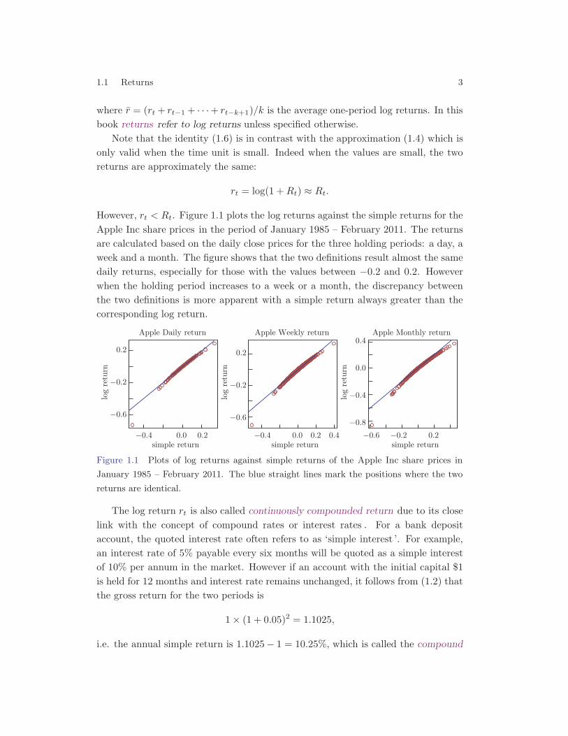
However, rt < Rt. Figure 1.1 plots the log returns against the simple returns for theApple Inc share prices in the period of January 1985 – February 2011. The returnsare calculated based on the daily close prices for the three holding periods: a day, aweek and a month. The figure shows that the two definitions result almost the samedaily returns, especially for those with the values between −0.2 and 0.2. Howeverwhen the holding period increases to a week or a month, the discrepancy betweenthe two definitions is more apparent with a simple return always greater than thecorresponding log return.

Figure 1.1 Plots of log returns against simple returns of the Apple Inc share prices in

January 1985 – February 2011. The blue straight lines mark the positions where the two

returns are identical.

The log return rt is also called continuously compounded return due to its closelink with the concept of compound rates or interest rates . For a bank depositaccount, the quoted interest rate often refers to as ‘simple interest ’. For example,an interest rate of 5% payable every six months will be quoted as a simple interestof 10% per annum in the market. However if an account with the initial capital $1is held for 12 months and interest rate remains unchanged, it follows from (1.2) thatthe gross return for the two periods is

1× (1 + 0.05)2 = 1.1025,

i.e. the annual simple return is 1.1025− 1 = 10.25%, which is called the compound


return and is greater than the quoted annual rate of 10%. This is due to the earningfrom ‘interest-on-interest’ in the second six-month period.

Now suppose that the quoted simple interest rate per annum is r and is un-changed, and the earnings are paid more frequently, say, m times per annum (atthe rate r/m each time of course). For example, the account holder is paid everyquarter when m = 4, every month when m = 12, and every day when m = 365.Suppose m continues to increase, and the earnings are paid continuously eventually.Then the gross return at the end of one year is

limm→∞(1 + r/m)m = er.

More generally, if the initial capital is C, invested in a bond that compounds con-tinuously the interest at annual rate r, then the value of the investment at time tis

C exp(rt).

Hence the log return per annum is r, which is the logarithm of the gross return.This indicates that the simple annual interest rate r quoted in the market is in factthe annual log return if the interest is compounded continuously. Note that if theinterest is only paid once at the end of the year, the simple return will be r, and thelog return will be log(1 + r) which is always smaller than r.

In summary, a simple annual interest rate quoted in the market has two interpre-tations: it is the simple annual return if the interest is only paid once at the end ofthe year, and it is the annual log return if the interest is compounded continuously.

1.1.4 Adjustment for dividends

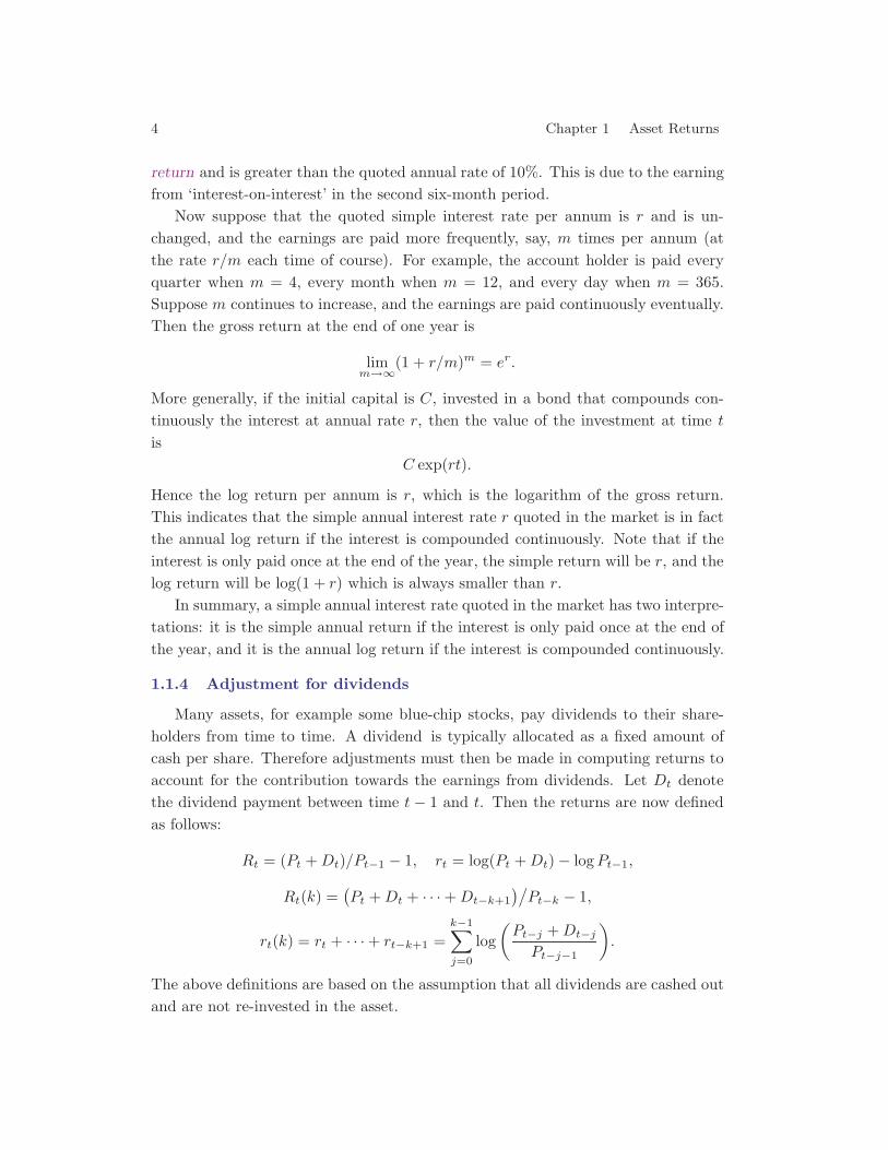
Many assets, for example some blue-chip stocks, pay dividends to their share-holders from time to time. A dividend is typically allocated as a fixed amount ofcash per share. Therefore adjustments must then be made in computing returns toaccount for the contribution towards the earnings from dividends. Let Dt denotethe dividend payment between time t − 1 and t. Then the returns are now definedas follows:

Rt = (Pt +Dt)/Pt−1 − 1, rt = log(Pt +Dt)− logPt−1,

Rt(k) =(Pt +Dt + · · ·+Dt−k+1

)/Pt−k − 1,

rt(k) = rt + · · ·+ rt−k+1 =k−1∑j=0

log(Pt−j +Dt−jPt−j−1

).

The above definitions are based on the assumption that all dividends are cashed outand are not re-invested in the asset.

1.1 Returns 5

1.1.5 Bond yields and prices

Bonds are quoted in annualized yields. A so-called zero-coupon bond is a bondbought at a price lower than its face value (also called par value or principal), withthe face value repaid at the time of maturity. It does not make periodic interestpayments (i.e. coupons), hence the term ‘zero-coupon’. Now we consider a zero-coupon bond with the face value $1. If the current yield is rt and the remainingduration is D units of time, with continuous compounding, its current price Bt

should satisfy the condition

Bt exp(Drt) = $1,

i.e. the price is Bt = exp(−Drt) dollars. Thus, the annualized log-return of thebond is

log(Bt+1/Bt) = D(rt − rt+1). (1.7)

Here, we ignore the fact that Bt+1 has one unit of time shorter maturity than Bt.

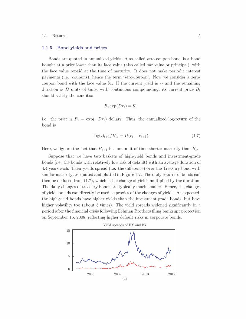
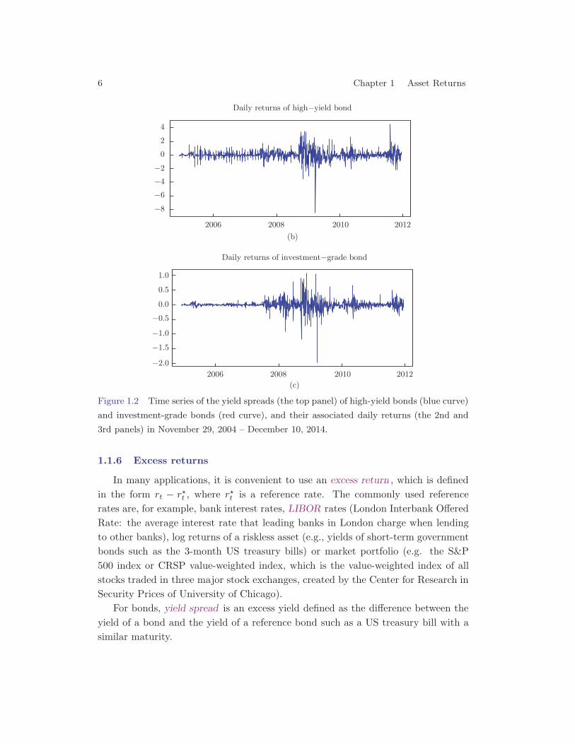
Suppose that we have two baskets of high-yield bonds and investment-gradebonds (i.e. the bonds with relatively low risk of default) with an average duration of4.4 years each. Their yields spread (i.e. the difference) over the Treasury bond withsimilar maturity are quoted and plotted in Figure 1.2. The daily returns of bonds canthen be deduced from (1.7), which is the change of yields multiplied by the duration.The daily changes of treasury bonds are typically much smaller. Hence, the changesof yield spreads can directly be used as proxies of the changes of yields. As expected,the high-yield bonds have higher yields than the investment grade bonds, but havehigher volatility too (about 3 times). The yield spreads widened significantly in aperiod after the financial crisis following Lehman Brothers filing bankrupt protectionon September 15, 2008, reflecting higher default risks in corporate bonds.


Figure 1.2 Time series of the yield spreads (the top panel) of high-yield bonds (blue curve)

and investment-grade bonds (red curve), and their associated daily returns (the 2nd and

3rd panels) in November 29, 2004 – December 10, 2014.

1.1.6 Excess returns

In many applications, it is convenient to use an excess return , which is definedin the form rt − r�t , where r

�t is a reference rate. The commonly used reference

rates are, for example, bank interest rates, LIBOR rates (London Interbank OfferedRate: the average interest rate that leading banks in London charge when lendingto other banks), log returns of a riskless asset (e.g., yields of short-term governmentbonds such as the 3-month US treasury bills) or market portfolio (e.g. the S&P500 index or CRSP value-weighted index, which is the value-weighted index of allstocks traded in three major stock exchanges, created by the Center for Research inSecurity Prices of University of Chicago).

For bonds, yield spread is an excess yield defined as the difference between theyield of a bond and the yield of a reference bond such as a US treasury bill with asimilar maturity.

1.2 Behavior of financial return data 7

1.2 Behavior of financial return data

In order to build useful statistical models for financial returns, we collect someempirical evidence first. To this end, we look into the daily closing indices of theS&P 500 and the daily closing share prices (in US dollars) of the Apple Inc in theperiod of January 1985 – February 2011. The data were adjusted for all splits anddividends, and were downloaded from Yahoo!Finance.

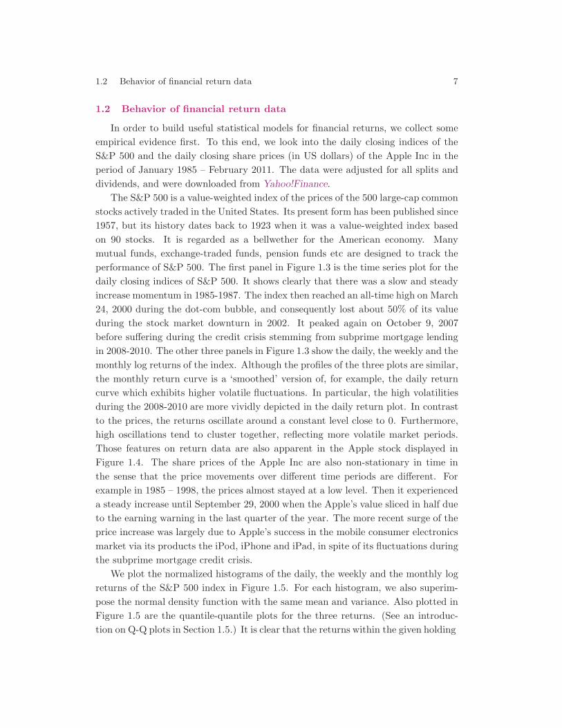
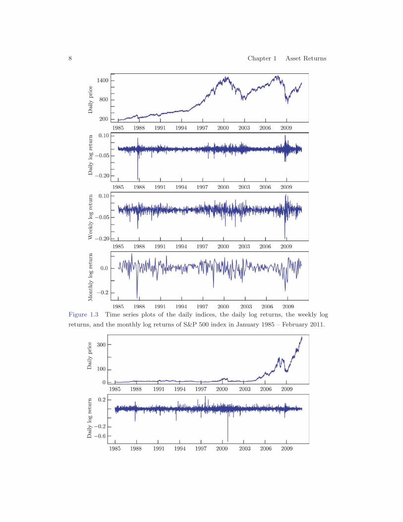
The S&P 500 is a value-weighted index of the prices of the 500 large-cap commonstocks actively traded in the United States. Its present form has been published since1957, but its history dates back to 1923 when it was a value-weighted index basedon 90 stocks. It is regarded as a bellwether for the American economy. Manymutual funds, exchange-traded funds, pension funds etc are designed to track theperformance of S&P 500. The first panel in Figure 1.3 is the time series plot for thedaily closing indices of S&P 500. It shows clearly that there was a slow and steadyincrease momentum in 1985-1987. The index then reached an all-time high on March24, 2000 during the dot-com bubble, and consequently lost about 50% of its valueduring the stock market downturn in 2002. It peaked again on October 9, 2007before suffering during the credit crisis stemming from subprime mortgage lendingin 2008-2010. The other three panels in Figure 1.3 show the daily, the weekly and themonthly log returns of the index. Although the profiles of the three plots are similar,the monthly return curve is a ‘smoothed’ version of, for example, the daily returncurve which exhibits higher volatile fluctuations. In particular, the high volatilitiesduring the 2008-2010 are more vividly depicted in the daily return plot. In contrastto the prices, the returns oscillate around a constant level close to 0. Furthermore,high oscillations tend to cluster together, reflecting more volatile market periods.Those features on return data are also apparent in the Apple stock displayed inFigure 1.4. The share prices of the Apple Inc are also non-stationary in time inthe sense that the price movements over different time periods are different. Forexample in 1985 – 1998, the prices almost stayed at a low level. Then it experienceda steady increase until September 29, 2000 when the Apple’s value sliced in half dueto the earning warning in the last quarter of the year. The more recent surge of theprice increase was largely due to Apple’s success in the mobile consumer electronicsmarket via its products the iPod, iPhone and iPad, in spite of its fluctuations duringthe subprime mortgage credit crisis.

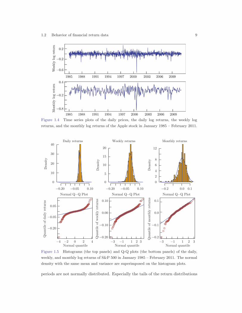
We plot the normalized histograms of the daily, the weekly and the monthly logreturns of the S&P 500 index in Figure 1.5. For each histogram, we also superim-pose the normal density function with the same mean and variance. Also plotted inFigure 1.5 are the quantile-quantile plots for the three returns. (See an introduc-tion on Q-Q plots in Section 1.5.) It is clear that the returns within the given holding


Figure 1.3 Time series plots of the daily indices, the daily log returns, the weekly log

returns, and the monthly log returns of S&P 500 index in January 1985 – February 2011.


Figure 1.4 Time series plots of the daily prices, the daily log returns, the weekly log

returns, and the monthly log returns of the Apple stock in January 1985 – February 2011.

Figure 1.5 Histograms (the top panels) and Q-Q plots (the bottom panels) of the daily,

weekly, and monthly log returns of S&P 500 in January 1985 – February 2011. The normal

density with the same mean and variance are superimposed on the histogram plots.

periods are not normally distributed. Especially the tails of the return distributions


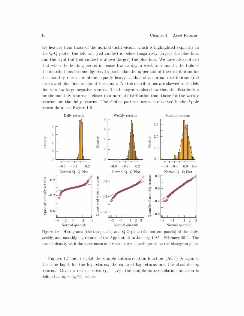
are heavier than those of the normal distribution, which is highlighted explicitly inthe Q-Q plots: the left tail (red circles) is below (negatively larger) the blue line,and the right tail (red circles) is above (larger) the blue line. We have also noticedthat when the holding period increases from a day, a week to a month, the tails ofthe distributions become lighter. In particular the upper tail of the distribution forthe monthly returns is about equally heavy as that of a normal distribution (redcircles and blue line are about the same). All the distributions are skewed to the leftdue to a few large negative returns. The histograms also show that the distributionfor the monthly returns is closer to a normal distribution than those for the weeklyreturns and the daily returns. The similar patterns are also observed in the Applereturn data; see Figure 1.6.

Figure 1.6 Histograms (the top panels) and Q-Q plots (the bottom panels) of the daily,

weekly, and monthly log returns of the Apple stock in January 1985 – February 2011. The

normal density with the same mean and variance are superimposed on the histogram plots.

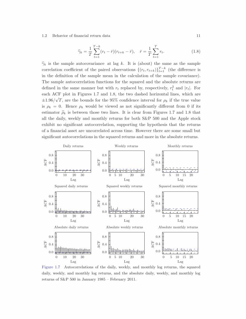
Figures 1.7 and 1.8 plot the sample autocorrelation function (ACF) ρ̂k againstthe time lag k for the log returns, the squared log returns and the absolute logreturns. Given a return series r1, · · · , rT , the sample autocorrelation function isdefined as ρ̂k = γ̂k/γ̂0, where


γ̂k =1T

T−k∑t=1

(rt − r̄)(rt+k − r̄), r̄ =1T

T∑t=1

rt. (1.8)

γ̂k is the sample autocovariance at lag k. It is (about) the same as the samplecorrelation coefficient of the paired observations {(rt, rt+k)}T−kt=1 (the difference isin the definition of the sample mean in the calculation of the sample covariance).The sample autocorrelation functions for the squared and the absolute returns aredefined in the same manner but with rt replaced by, respectively, r2t and |rt|. Foreach ACF plot in Figures 1.7 and 1.8, the two dashed horizontal lines, which are±1.96/√T , are the bounds for the 95% confidence interval for ρk if the true valueis ρk = 0. Hence ρk would be viewed as not significantly different from 0 if itsestimator ρ̂k is between those two lines. It is clear from Figures 1.7 and 1.8 thatall the daily, weekly and monthly returns for both S&P 500 and the Apple stockexhibit no significant autocorrelation, supporting the hypothesis that the returnsof a financial asset are uncorrelated across time. However there are some small butsignificant autocorrelations in the squared returns and more in the absolute returns.

Figure 1.7 Autocorrelations of the daily, weekly, and monthly log returns, the squared

daily, weekly, and monthly log returns, and the absolute daily, weekly, and monthly log

returns of S&P 500 in January 1985 – February 2011.


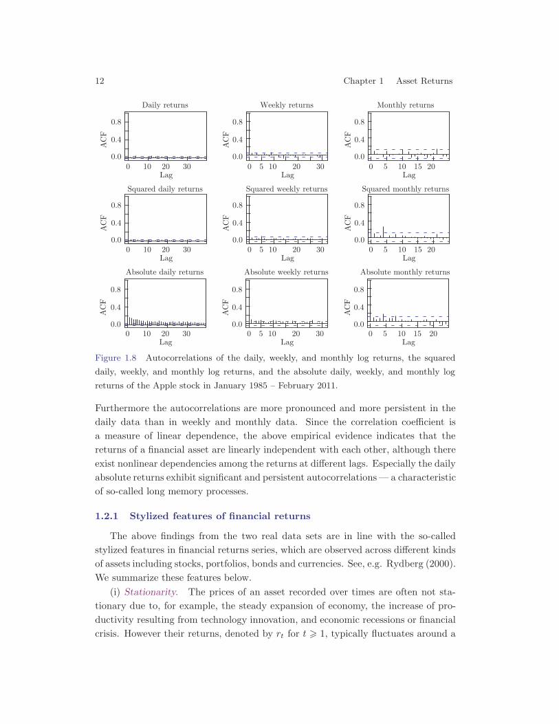
Figure 1.8 Autocorrelations of the daily, weekly, and monthly log returns, the squared

daily, weekly, and monthly log returns, and the absolute daily, weekly, and monthly log

returns of the Apple stock in January 1985 – February 2011.

Furthermore the autocorrelations are more pronounced and more persistent in thedaily data than in weekly and monthly data. Since the correlation coefficient isa measure of linear dependence, the above empirical evidence indicates that thereturns of a financial asset are linearly independent with each other, although thereexist nonlinear dependencies among the returns at different lags. Especially the dailyabsolute returns exhibit significant and persistent autocorrelations— a characteristicof so-called long memory processes.

1.2.1 Stylized features of financial returns

The above findings from the two real data sets are in line with the so-calledstylized features in financial returns series, which are observed across different kindsof assets including stocks, portfolios, bonds and currencies. See, e.g. Rydberg (2000).We summarize these features below.

(i) Stationarity. The prices of an asset recorded over times are often not sta-tionary due to, for example, the steady expansion of economy, the increase of pro-ductivity resulting from technology innovation, and economic recessions or financialcrisis. However their returns, denoted by rt for t � 1, typically fluctuates around a


constant level, suggesting a constant mean over time. See Figures 1.3 and 1.4. Infact most return sequences can be modeled as a stochastic processes with at leasttime-invariant first two moments (i.e. the weak stationarity; see 2.1). A simple(and perhaps over-simplistic) approach is to assume that all the finite dimensionaldistributions of a return sequence are time-invariant.

(ii) Heavy tails. The probability distribution of return rt often exhibits heaviertails than those of a normal distribution. Figures 1.5 and 1.6 provide the quantile-

quantile plot or Q-Q plot for graphical checking of normality. See Section 1.5 for de-tail. A frequently used statistic for checking the normality (including tail-heaviness)is the Jarque-Bera test presented in Section 1.5. Nevertheless rt is assumed typicallyto have at least two finite moments (i.e. E(r2t ) <∞), although it is debatable howmany moments actually exist for a given asset.

The density of t-distribution with degree of freedom ν is given by

fν(x) = d−1ν

(1 +

x2

ν

)−(ν+1)/2

, (1.9)

where dν = B(0.5, 0.5ν)√ν is the normalization constant and B is a beta function.

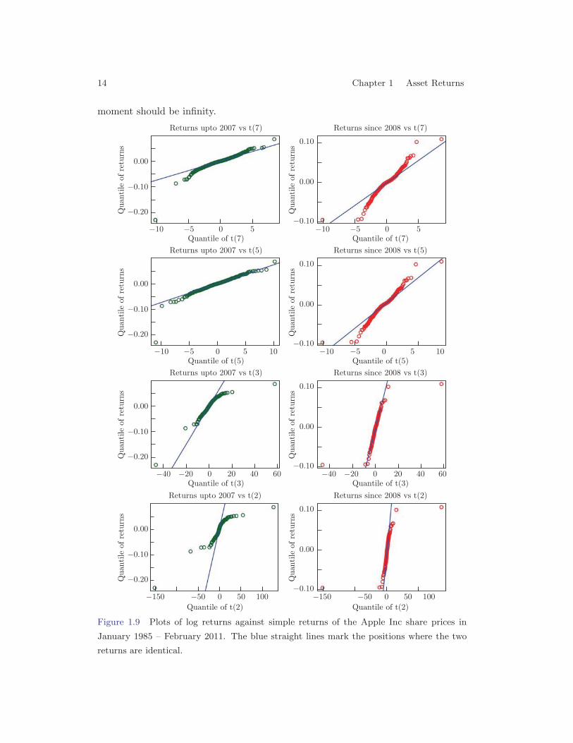
This distribution is often denoted as t(ν) or tν . Its tails are of polynomial orderfν(x) � |x|−(ν+1) (as |x| → ∞), which are heavier than the normal density. Notethat for any random variable X ∼ t(ν), E{|X |ν} =∞ and E{|X |ν−δ} <∞ for anyδ ∈ (0, ν].When ν is large, t(v) is close to a normal distribution. In fact, based on a sam-ple of size 2500 (approximately 10-year daily data), one can not differentiate t(10)from a normal distribution based on, for example, the Kolmogorov-Smirnov test(the function KS.test in R). However their tail behaviors are very different: A5-standard-deviation (SD) event occurs once in every 14000 years under a normaldistribution, once in every 15 years under t10, and once in every 1.5 years undert4.5. The calculation goes as follows. The probability of getting a −5 SD daily shockor worse under the normal distribution is 2.8665 × 10−7 (which is P (Z < −5) forZ ∼ N(0, 1)), or 1 in 3488575 days. Dividing this by approximately 252 tradingdays per year yields the result of 13844 years. A similar calculation can be donewith different kinds of t-distributions. If the tails of stock returns behave like t4.5,the left tail of typical daily S&P 500 returns, the occurrence of −5 SD event is moreoften than what we would conceive.Figure 1.9 plots the quantiles of the S&P 500 returns in the period January 1985– February 2011 against the quantiles of t(ν) distributions with ν = 2, 3, · · · , 7. Itis clear that the tails of the S&P 500 return are heavier than the tails of t(5), andare thinner than the tails of t(2) (and perhaps also t(3)). Hence it is reasonable toassume that the second moment of the return of the S&P 500 is finite while the 5th


moment should be infinity.

Figure 1.9 Plots of log returns against simple returns of the Apple Inc share prices in

January 1985 – February 2011. The blue straight lines mark the positions where the two

returns are identical.


(iii) Asymmetry. The distribution of return rt is often negatively skewed (Figures1.5 and 1.6), reflecting the fact that the downturns of financial markets are oftenmuch steeper than the recoveries. Investors tend to react more strongly to negativenews than to positive news.

(iv) Volatility clustering. This term refers to the fact that large price changes(i.e. returns with large absolute values) occur in clusters. See Figures 1.3 and 1.4.Indeed, large price changes tend to be followed by large price changes, and periodsof tranquility alternate with periods of high volatility. The time varying volatilitycan easily be see in Figures 1.3. The standard deviation of S&P 500 returns fromNovember 29, 2004 to December 31, 2007 (3 months before JP Morgan Chase offeredto acquire Bear Stearns at a price of $2 per share on March 17, 2008) is 0.78%, andthe standard deviation of the returns since 2008 is 1.83%. The volatility of S&P 500in 2005 and 2006 is merely 0.64%, whereas the volatility at the height of the 2008financial crisis (September 15, 2008 to March 16, 2009, i.e. from a month before to6 months after Lehmann Brother’s fall) is 3.44%.

(v) Aggregational Gaussianity. Note that a return over k days is simply theaggregation of k daily returns; see (1.6). When the time horizon increases, thecentral limit law sets in and the distribution of the returns over a long time-horizon(such as a month) tends toward a normal distribution. See Figures 1.5 and 1.6.

(vi) Long range dependence. The returns themselves hardly show any serialcorrelation, which, however, does not mean that they are independent. In fact, bothdaily squared and absolute returns often exhibit small and significant autocorrela-tions. Those autocorrelations are persistent for absolute returns, indicating possiblelong-memory properties. It is also noticeable that those autocorrelations becomeweaker and less persistent when the sampling interval is increased from a day, to aweek to a month. See Figure 1.7.

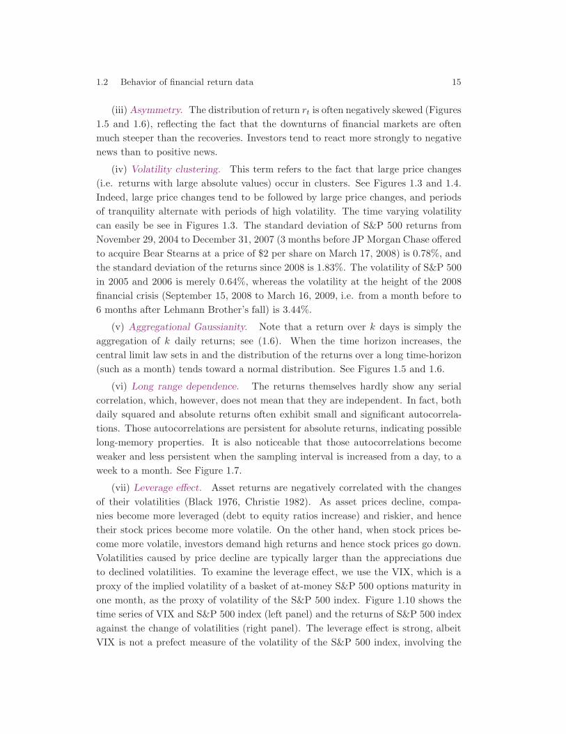
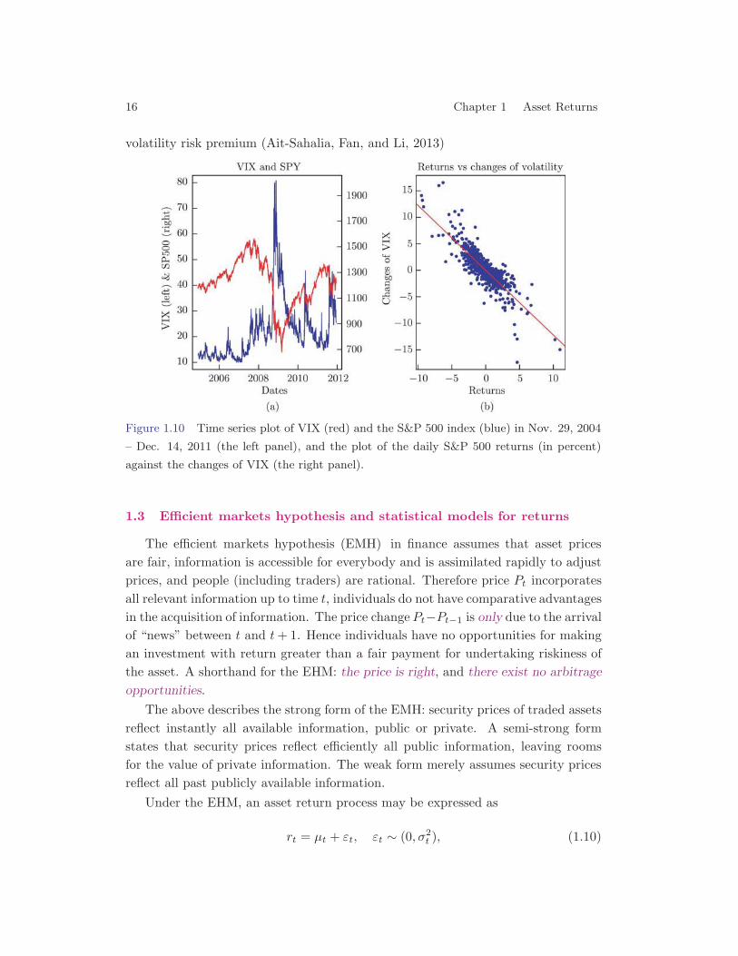
(vii) Leverage effect. Asset returns are negatively correlated with the changesof their volatilities (Black 1976, Christie 1982). As asset prices decline, compa-nies become more leveraged (debt to equity ratios increase) and riskier, and hencetheir stock prices become more volatile. On the other hand, when stock prices be-come more volatile, investors demand high returns and hence stock prices go down.Volatilities caused by price decline are typically larger than the appreciations dueto declined volatilities. To examine the leverage effect, we use the VIX, which is aproxy of the implied volatility of a basket of at-money S&P 500 options maturity inone month, as the proxy of volatility of the S&P 500 index. Figure 1.10 shows thetime series of VIX and S&P 500 index (left panel) and the returns of S&P 500 indexagainst the change of volatilities (right panel). The leverage effect is strong, albeitVIX is not a prefect measure of the volatility of the S&P 500 index, involving the


volatility risk premium (Ait-Sahalia, Fan, and Li, 2013)

Figure 1.10 Time series plot of VIX (red) and the S&P 500 index (blue) in Nov. 29, 2004

– Dec. 14, 2011 (the left panel), and the plot of the daily S&P 500 returns (in percent)

against the changes of VIX (the right panel).

1.3 Efficient markets hypothesis and statistical models for returns

The efficient markets hypothesis (EMH) in finance assumes that asset pricesare fair, information is accessible for everybody and is assimilated rapidly to adjustprices, and people (including traders) are rational. Therefore price Pt incorporatesall relevant information up to time t, individuals do not have comparative advantagesin the acquisition of information. The price change Pt−Pt−1 is only due to the arrivalof “news” between t and t+ 1. Hence individuals have no opportunities for makingan investment with return greater than a fair payment for undertaking riskiness ofthe asset. A shorthand for the EHM: the price is right, and there exist no arbitrage

opportunities.The above describes the strong form of the EMH: security prices of traded assets

reflect instantly all available information, public or private. A semi-strong formstates that security prices reflect efficiently all public information, leaving roomsfor the value of private information. The weak form merely assumes security pricesreflect all past publicly available information.

Under the EHM, an asset return process may be expressed as

rt = μt + εt, εt ∼ (0, σ2t ), (1.10)

1.3 Efficient markets hypothesis and statistical models for returns 17

where μt is the rational expectation of rt at time t− 1, and εt represents the returndue to unpredictable “news” which arrives between time t − 1 and t. In this sense,εt is an innovation – a term used very often in time series literature. We use thenotation X ∼ (μ, ν) to denote that a random variable X has mean μ and varianceν, respectively. The assumption that Eεt = 0 reflects the belief that on average theactual change of log price equals the expectation μt.

By combining the EHM model (1.10) with some stylized features outlined inSection 1.2, most frequently used statistical models for financial returns admit theform

rt = μ+ εt, εt ∼WN(0, σ2), (1.11)

where μ = Ert is the expected return, which is assumed to be a constant. Thenotation εt ∼ WN(0, σ2) denotes that ε1, ε2, · · · form a white noise process withEεt = 0 and var(εt) = σ2; see (i) below. Here we assume that var(εt) = var(rt) = σ2

is a finite positive constant, noting that most varying volatilities in the return plotsin Figures 1.3 & 1.4 can be represented by conditional heteroscadasticity under themartingale difference assumption (ii) below. The assumption (1.11) is reasonable,supported by the empirical analysis in section 1.2.

There are three different types of assumptions about the innovations {εt} in(1.11), from the weakest to the strongest.

(i) White noise innovations : {εt} are white noise, denoted as εt ∼ WN(0, σ2).Under this assumption, Corr(εt, εs) = 0 for all t = s.

(ii) Martingale difference innovations : εt form a martingale difference sequencein the sense that for any t

E(εt|rt−1, rt−2, · · · ) = E(εt|εt−1, εt−2, · · · ) = 0. (1.12)

One of the most frequently used format for martingale difference innovations is ofthe form

εt = σtηt, (1.13)

where ηt ∼ IID(0, 1) (see (iii) below), and σt is a predictable volatility process,known at time t− 1, satisfying the condition

E(σt|rt−1, rt−2, · · · ) = σt.

Note that ARCH and GARCH processes are special cases of (1.13).(iii) IID innovations : εt are independent and identically distributed, denoted as

εt ∼ IID(0, σ2).The assumption of IID innovations is the strongest. It implies that the innovationsare martingale differences. On the other hand, if {εt} satisfies (1.12), it holds that


for any t > s,

cov(εt, εs) = E(εtεs) = E{E(εtεs|εt−1, εt−2, · · · )}= E{εsE(εt|εt−1, εt−2, · · · )} = 0.

Hence, {εt} is a white noise series. Therefore the relationship among the three typesof innovations is as follows:

IID ⇒ Martingale differences ⇒ White noise.

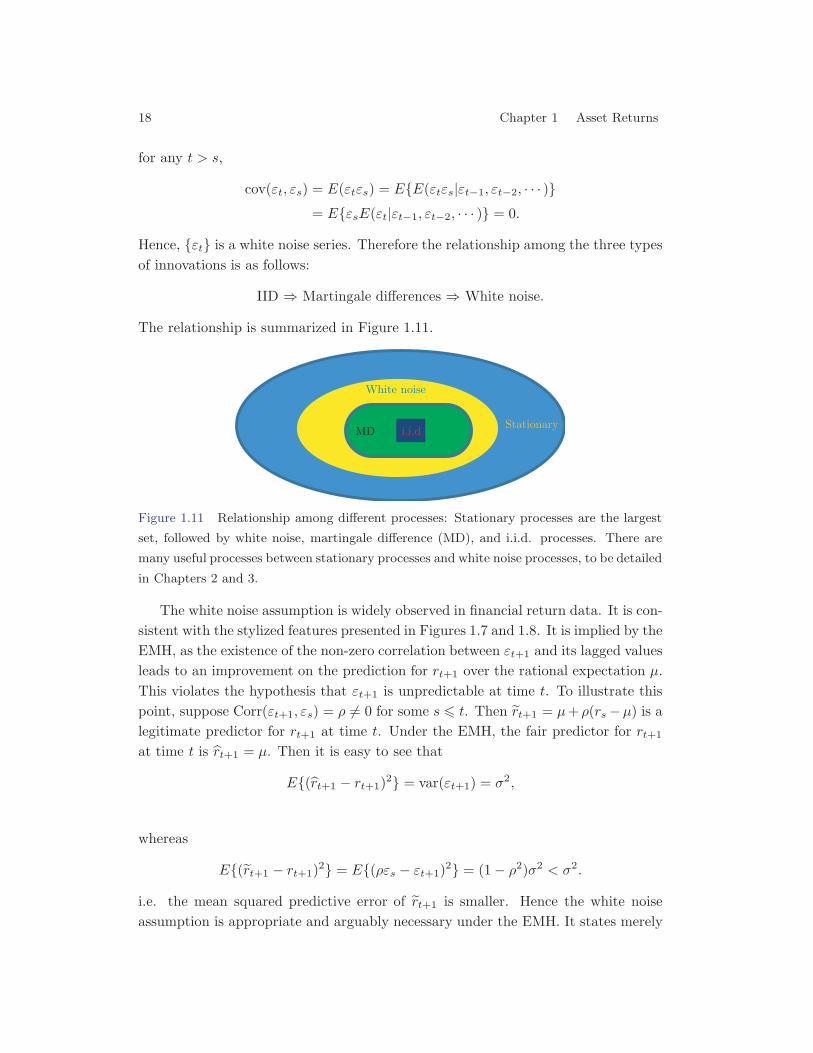
The relationship is summarized in Figure 1.11.

Figure 1.11 Relationship among different processes: Stationary processes are the largest

set, followed by white noise, martingale difference (MD), and i.i.d. processes. There are

many useful processes between stationary processes and white noise processes, to be detailed

in Chapters 2 and 3.

The white noise assumption is widely observed in financial return data. It is con-sistent with the stylized features presented in Figures 1.7 and 1.8. It is implied by theEMH, as the existence of the non-zero correlation between εt+1 and its lagged valuesleads to an improvement on the prediction for rt+1 over the rational expectation μ.This violates the hypothesis that εt+1 is unpredictable at time t. To illustrate thispoint, suppose Corr(εt+1, εs) = ρ = 0 for some s � t. Then r̃t+1 = μ+ ρ(rs−μ) is alegitimate predictor for rt+1 at time t. Under the EMH, the fair predictor for rt+1

at time t is r̂t+1 = μ. Then it is easy to see that

E{(r̂t+1 − rt+1)2} = var(εt+1) = σ2,

whereas

E{(r̃t+1 − rt+1)2} = E{(ρεs − εt+1)2} = (1− ρ2)σ2 < σ2.

i.e. the mean squared predictive error of r̃t+1 is smaller. Hence the white noiseassumption is appropriate and arguably necessary under the EMH. It states merely

1.3 Efficient markets hypothesis and statistical models for returns 19

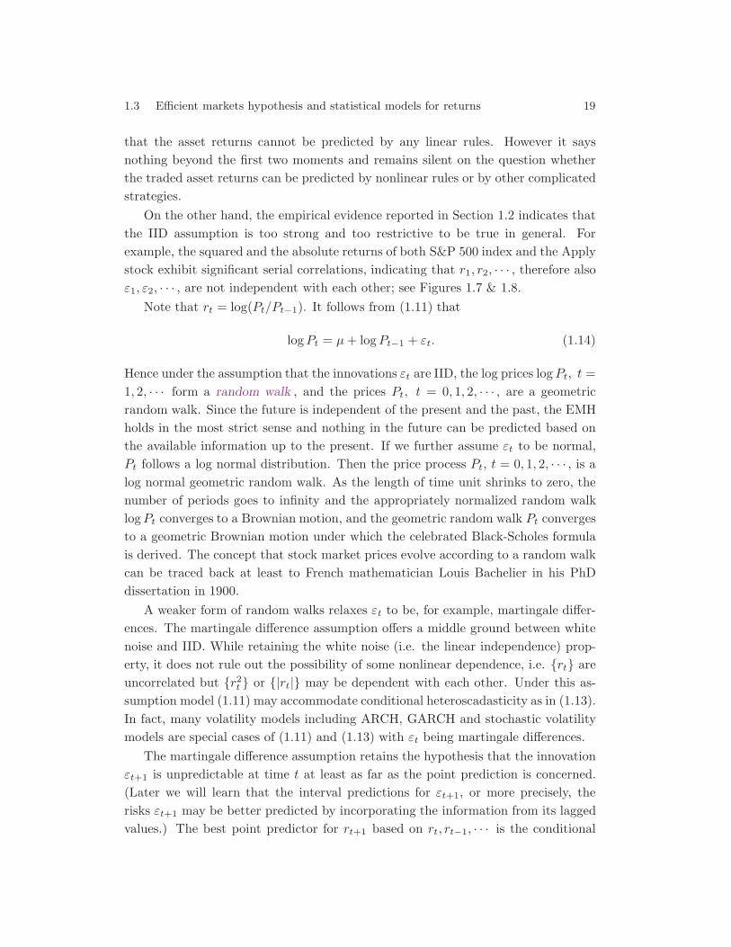
that the asset returns cannot be predicted by any linear rules. However it saysnothing beyond the first two moments and remains silent on the question whetherthe traded asset returns can be predicted by nonlinear rules or by other complicatedstrategies.

On the other hand, the empirical evidence reported in Section 1.2 indicates thatthe IID assumption is too strong and too restrictive to be true in general. Forexample, the squared and the absolute returns of both S&P 500 index and the Applystock exhibit significant serial correlations, indicating that r1, r2, · · · , therefore alsoε1, ε2, · · · , are not independent with each other; see Figures 1.7 & 1.8.

Note that rt = log(Pt/Pt−1). It follows from (1.11) that

logPt = μ+ logPt−1 + εt. (1.14)

Hence under the assumption that the innovations εt are IID, the log prices logPt, t =1, 2, · · · form a random walk , and the prices Pt, t = 0, 1, 2, · · · , are a geometricrandom walk. Since the future is independent of the present and the past, the EMHholds in the most strict sense and nothing in the future can be predicted based onthe available information up to the present. If we further assume εt to be normal,Pt follows a log normal distribution. Then the price process Pt, t = 0, 1, 2, · · · , is alog normal geometric random walk. As the length of time unit shrinks to zero, thenumber of periods goes to infinity and the appropriately normalized random walklogPt converges to a Brownian motion, and the geometric random walk Pt convergesto a geometric Brownian motion under which the celebrated Black-Scholes formulais derived. The concept that stock market prices evolve according to a random walkcan be traced back at least to French mathematician Louis Bachelier in his PhDdissertation in 1900.

A weaker form of random walks relaxes εt to be, for example, martingale differ-ences. The martingale difference assumption offers a middle ground between whitenoise and IID. While retaining the white noise (i.e. the linear independence) prop-erty, it does not rule out the possibility of some nonlinear dependence, i.e. {rt} areuncorrelated but {r2t } or {|rt|} may be dependent with each other. Under this as-sumption model (1.11) may accommodate conditional heteroscadasticity as in (1.13).In fact, many volatility models including ARCH, GARCH and stochastic volatilitymodels are special cases of (1.11) and (1.13) with εt being martingale differences.

The martingale difference assumption retains the hypothesis that the innovationεt+1 is unpredictable at time t at least as far as the point prediction is concerned.(Later we will learn that the interval predictions for εt+1, or more precisely, therisks εt+1 may be better predicted by incorporating the information from its laggedvalues.) The best point predictor for rt+1 based on rt, rt−1, · · · is the conditional


expectation

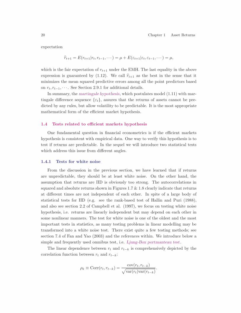
r̂t+1 = E(rt+1|rt, rt−1, · · · ) = μ+ E(εt+1|εt, εt−1, · · · ) = μ,

which is the fair expectation of rt+1 under the EMH. The last equality in the aboveexpression is guaranteed by (1.12). We call r̂t+1 as the best in the sense that itminimizes the mean squared predictive errors among all the point predictors basedon rt, rt−1, · · · . See Section 2.9.1 for additional details.

In summary, the martingale hypothesis, which postulates model (1.11) with mar-tingale difference sequence {εt}, assures that the returns of assets cannot be pre-dicted by any rules, but allow volatility to be predictable. It is the most appropriatemathematical form of the efficient market hypothesis.

1.4 Tests related to efficient markets hypothesis

One fundamental question in financial econometrics is if the efficient marketshypothesis is consistent with empirical data. One way to verify this hypothesis is totest if returns are predictable. In the sequel we will introduce two statistical testswhich address this issue from different angles.

1.4.1 Tests for white noise

From the discussion in the previous section, we have learned that if returnsare unpredictable, they should be at least white noise. On the other hand, theassumption that returns are IID is obviously too strong. The autocorrelations insquared and absolute returns shown in Figures 1.7 & 1.8 clearly indicate that returnsat different times are not independent of each other. In spite of a large body ofstatistical tests for IID (e.g. see the rank-based test of Hallin and Puri (1988),and also see section 2.2 of Campbell et al. (1997), we focus on testing white noisehypothesis, i.e. returns are linearly independent but may depend on each other insome nonlinear manners. The test for white noise is one of the oldest and the mostimportant tests in statistics, as many testing problems in linear modelling may betransformed into a white noise test. There exist quite a few testing methods; seesection 7.4 of Fan and Yao (2003) and the references within. We introduce below asimple and frequently used omnibus test, i.e. Ljung-Box portmanteau test .

The linear dependence between rt and rt−k is comprehensively depicted by thecorrelation function between rt and rt−k:

ρk ≡ Corr(rt, rt−k) = cov(rt, rt−k)√var(rt)var(rt−k)

.

1.4 Tests related to efficient markets hypothesis 21

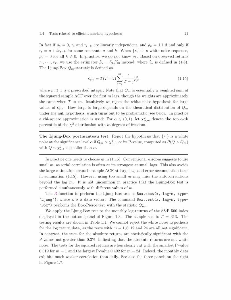
In fact if ρk = 0, rt and rt−k are linearly independent, and ρk = ±1 if and only ifrt = a + brt−k for some constants a and b. When {rt} is a white noise sequence,ρk = 0 for all k = 0. In practice, we do not know ρk. Based on observed returnsr1, · · · , rT , we use the estimator ρ̂k = γ̂k/γ̂0 instead, where γ̂k is defined in (1.8).The Ljung-Box Qm-statistic is defined as

Qm = T (T + 2)m∑j=1

1T − j

ρ̂2j , (1.15)

where m � 1 is a prescribed integer. Note that Qm is essentially a weighted sum ofthe squared sample ACF over the first m lags, though the weights are approximatelythe same when T � m. Intuitively we reject the white noise hypothesis for largevalues of Qm. How large is large depends on the theoretical distribution of Qm

under the null hypothesis, which turns out to be problematic; see below. In practicea chi-square approximation is used: For α ∈ (0, 1), let χ2α,m denote the top α-thpercentile of the χ2-distribution with m degrees of freedom.

The Ljung-Box portmanteau test: Reject the hypothesis that {rt} is a whitenoise at the significance level α ifQm > χ2α,m or its P-value, computed as P (Q > Qm)with Q ∼ χ2m, is smaller than α.

In practice one needs to choosem in (1.15). Conventional wisdom suggests to usesmall m, as serial correlation is often at its strongest at small lags. This also avoidsthe large estimation errors in sample ACF at large lags and error accumulation issuein summation (1.15). However using too small m may miss the autocorrelationsbeyond the lag m. It is not uncommon in practice that the Ljung-Box test isperformed simultaneously with different values of m.

The R-function to perform the Ljung-Box test is Box.test(x, lag=m, type=

"Ljung"), where x is a data vector. The command Box.test(x, lag=m, type=

"Box") performs the Box-Pierce test with the statistic Q∗m.We apply the Ljung-Box test to the monthly log returns of the S&P 500 index

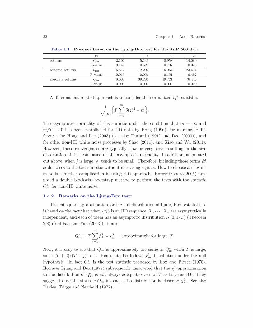
displayed in the bottom panel of Figure 1.3. The sample size is T = 313. Thetesting results are shown in Table 1.1. We cannot reject the white noise hypothesisfor the log return data, as the tests with m = 1, 6, 12 and 24 are all not significant.In contrast, the tests for the absolute returns are statistically significant with theP-values not greater than 0.3%, indicating that the absolute returns are not whitenoise. The tests for the squared returns are less clearly cut with the smallest P-value0.019 for m = 1 and the largest P-value 0.492 for m = 24. Indeed, the monthly dataexhibits much weaker correlation than daily. See also the three panels on the rightin Figure 1.7.


Table 1.1 P-values based on the Ljung-Box test for the S&P 500 data

m 1 6 12 24

returns Qm 2.101 5.149 8.958 14.080

P-value 0.147 0.525 0.707 0.945

squared returns Qm 5.517 12.292 16.964 23.474

P-value 0.019 0.056 0.151 0.492

absolute returns Qm 8.687 39.283 49.721 76.446

P-value 0.003 0.000 0.000 0.000

A different but related approach is to consider the normalized Q∗m-statistic:

1√2m

{T

m∑j=1

ρ̂(j)2 −m}.

The asymptotic normality of this statistic under the condition that m → ∞ andm/T → 0 has been established for IID data by Hong (1996), for martingale dif-ferences by Hong and Lee (2003) (see also Durlauf (1991) and Deo (2000)), andfor other non-IID white noise processes by Shao (2011), and Xiao and Wu (2011).However, those convergences are typically slow or very slow, resulting in the sizedistortation of the tests based on the asymptotic normality. In addition, as pointedout above, when j is large, ρj tends to be small. Therefore, including those terms ρ̂2jadds noises to the test statistic without increasing signals. How to choose a relevantm adds a further complication in using this approach. Horowitz et al.(2006) pro-posed a double blockwise bootstrap method to perform the tests with the statisticQ∗m for non-IID white noise.

1.4.2 Remarks on the Ljung-Box test∗

The chi-square approximation for the null distribution of Ljung-Box test statisticis based on the fact that when {rt} is an IID sequence, ρ̂1, · · · , ρ̂m are asymptoticallyindependent, and each of them has an asymptotic distribution N(0, 1/T ) (Theorem2.8(iii) of Fan and Yao (2003)). Hence

Q∗m ≡ T

m∑j=1

ρ̂2j ∼ χ2m approximately for large T.

Now, it is easy to see that Qm is approximately the same as Q∗m when T is large,since (T + 2)/(T − j) ≈ 1. Hence, it also follows χ2m-distribution under the nullhypothesis. In fact Q∗m is the test statistic proposed by Box and Pierce (1970).However Ljung and Box (1978) subsequently discovered that the χ2-approximationto the distribution of Q∗m is not always adequate even for T as large as 100. Theysuggest to use the statistic Qm instead as its distribution is closer to χ2m. See alsoDavies, Triggs and Newbold (1977).


A more fundamental problem in applying the Ljung-Box test is that the statisticitself is defined to detecting the departure from white noise, but the asymptoticχ2-distribution can only be justified under the IID assumption. Therefore, as for-mulated above, it should not be used to test the hypothesis that the returns arewhite noise but not IID, as then the asymptotic null distributions of ρ̂(k) depend onthe high moments of the underlying distribution of rt. These asymptotic null dis-tributions may typically be too complicated to be directly useful in the sense thatthe asymptotic null distributions of Qm or Q∗m may then not be of the known formsfor fixed m; see, e.g. Romano and Thombs (1996). Unfortunately this problem alsoapplies to most (if not all) other omnibus white noise tests.

One alternative is to impose an explicit assumption on the structure of whitenoise process (such as a GARCH structure), then some resampling methods may beemployed to simulate the null distribution of Qm. Furthermore if one is also willingto impose some assumptions on the parametric form of a possible departure fromwhite noise, a likelihood ratio test can be employed, which is often more powerfulthan a omnibus nonparametric test, as the latter tries to detect the departure (fromwhite noise) to all different possibilities. The analogy is that an all-purpose tool istypically less powerful on a particular task than a customized tool. An example ofthe customized tool is the Dicky-Fuller test in the next section. However it itselfis a challenge to find relevant assumptions. This is why omnibus tests such as theLjung-Box test are often used in practice, in spite of their potential problems inmispecifying significance levels.

1.4.3 Tests for random walks

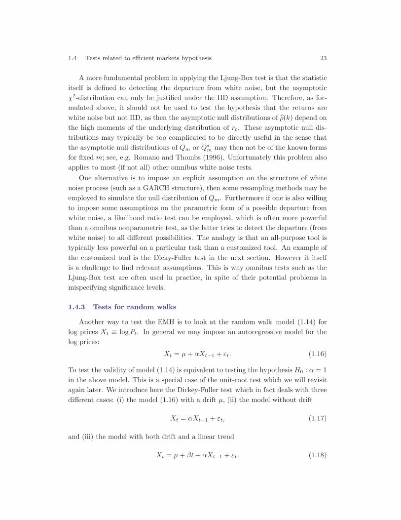
Another way to test the EMH is to look at the random walk model (1.14) forlog prices Xt ≡ logPt. In general we may impose an autoregressive model for thelog prices:

Xt = μ+ αXt−1 + εt. (1.16)

To test the validity of model (1.14) is equivalent to testing the hypothesis H0 : α = 1in the above model. This is a special case of the unit-root test which we will revisitagain later. We introduce here the Dickey-Fuller test which in fact deals with threedifferent cases: (i) the model (1.16) with a drift μ, (ii) the model without drift

Xt = αXt−1 + εt, (1.17)

and (iii) the model with both drift and a linear trend

Xt = μ+ βt+ αXt−1 + εt. (1.18)


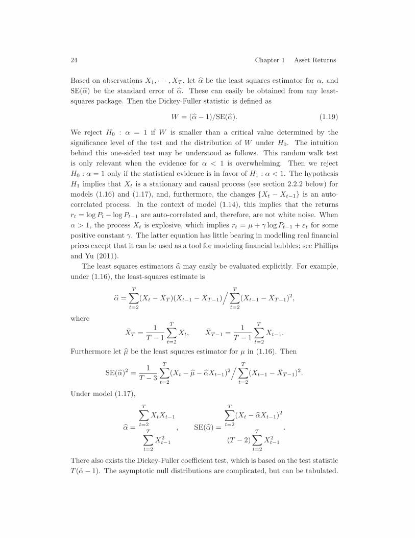
Based on observations X1, · · · , XT , let α̂ be the least squares estimator for α, andSE(α̂) be the standard error of α̂. These can easily be obtained from any least-squares package. Then the Dickey-Fuller statistic is defined as

W = (α̂− 1)/SE(α̂). (1.19)

We reject H0 : α = 1 if W is smaller than a critical value determined by thesignificance level of the test and the distribution of W under H0. The intuitionbehind this one-sided test may be understood as follows. This random walk testis only relevant when the evidence for α < 1 is overwhelming. Then we rejectH0 : α = 1 only if the statistical evidence is in favor of H1 : α < 1. The hypothesisH1 implies that Xt is a stationary and causal process (see section 2.2.2 below) formodels (1.16) and (1.17), and, furthermore, the changes {Xt − Xt−1} is an auto-correlated process. In the context of model (1.14), this implies that the returnsrt = logPt − logPt−1 are auto-correlated and, therefore, are not white noise. Whenα > 1, the process Xt is explosive, which implies rt = μ + γ logPt−1 + εt for somepositive constant γ. The latter equation has little bearing in modelling real financialprices except that it can be used as a tool for modeling financial bubbles; see Phillipsand Yu (2011).

The least squares estimators α̂ may easily be evaluated explicitly. For example,under (1.16), the least-squares estimate is

α̂ =T∑t=2

(Xt − X̄T )(Xt−1 − X̄T−1)/ T∑

t=2

(Xt−1 − X̄T−1)2,

where

X̄T =1

T − 1T∑t=2

Xt, X̄T−1 =1

T − 1T∑t=2

Xt−1.

Furthermore let μ̂ be the least squares estimator for μ in (1.16). Then

SE(α̂)2 =1

T − 3T∑t=2

(Xt − μ̂− α̂Xt−1)2/ T∑

t=2

(Xt−1 − X̄T−1)2.

Under model (1.17),

α̂ =

T∑t=2

XtXt−1

T∑t=2

X2t−1

, SE(α̂) =

T∑t=2

(Xt − α̂Xt−1)2

(T − 2)T∑t=2

X2t−1

.

There also exists the Dickey-Fuller coefficient test, which is based on the test statisticT (α̂− 1). The asymptotic null distributions are complicated, but can be tabulated.


At significant level α = 0.05, the critical values are −8.347 and −13.96 respectivelyfor testing model (1.17) (without drift) and model (1.16) (with drift).

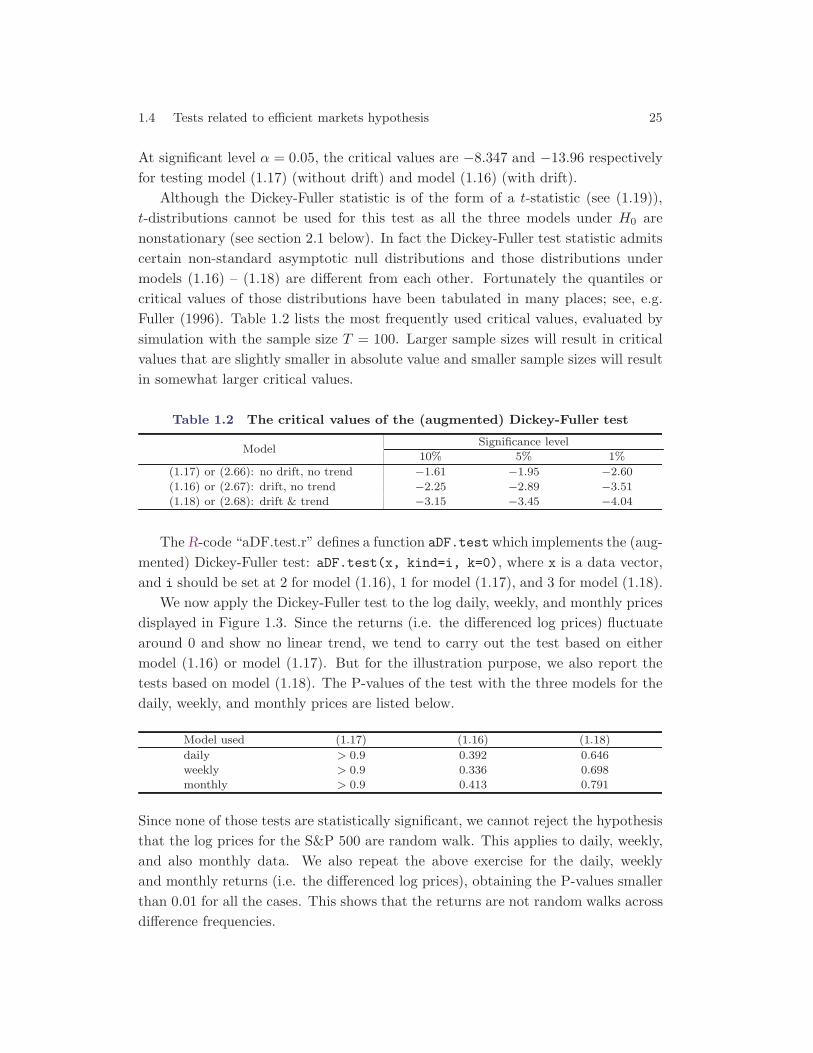
Although the Dickey-Fuller statistic is of the form of a t-statistic (see (1.19)),t-distributions cannot be used for this test as all the three models under H0 arenonstationary (see section 2.1 below). In fact the Dickey-Fuller test statistic admitscertain non-standard asymptotic null distributions and those distributions undermodels (1.16) – (1.18) are different from each other. Fortunately the quantiles orcritical values of those distributions have been tabulated in many places; see, e.g.Fuller (1996). Table 1.2 lists the most frequently used critical values, evaluated bysimulation with the sample size T = 100. Larger sample sizes will result in criticalvalues that are slightly smaller in absolute value and smaller sample sizes will resultin somewhat larger critical values.

Table 1.2 The critical values of the (augmented) Dickey-Fuller test

ModelSignificance level

10% 5% 1%

(1.17) or (2.66): no drift, no trend −1.61 −1.95 −2.60

(1.16) or (2.67): drift, no trend −2.25 −2.89 −3.51

(1.18) or (2.68): drift & trend −3.15 −3.45 −4.04

TheR-code “aDF.test.r” defines a function aDF.testwhich implements the (aug-mented) Dickey-Fuller test: aDF.test(x, kind=i, k=0), where x is a data vector,and i should be set at 2 for model (1.16), 1 for model (1.17), and 3 for model (1.18).

We now apply the Dickey-Fuller test to the log daily, weekly, and monthly pricesdisplayed in Figure 1.3. Since the returns (i.e. the differenced log prices) fluctuatearound 0 and show no linear trend, we tend to carry out the test based on eithermodel (1.16) or model (1.17). But for the illustration purpose, we also report thetests based on model (1.18). The P-values of the test with the three models for thedaily, weekly, and monthly prices are listed below.

Model used (1.17) (1.16) (1.18)

daily > 0.9 0.392 0.646

weekly > 0.9 0.336 0.698

monthly > 0.9 0.413 0.791

Since none of those tests are statistically significant, we cannot reject the hypothesisthat the log prices for the S&P 500 are random walk. This applies to daily, weekly,and also monthly data. We also repeat the above exercise for the daily, weeklyand monthly returns (i.e. the differenced log prices), obtaining the P-values smallerthan 0.01 for all the cases. This shows that the returns are not random walks acrossdifference frequencies.


The Dickey-Fuller test was originally proposed in Dickey and Fuller (1979). It hasbeen further adapted in handling the situations when there are some autoregressiveterms in models(1.16) – (1.18); see section 2.8.2 below.

1.4.4 Ljung-Box test and Dickey-Fuller test

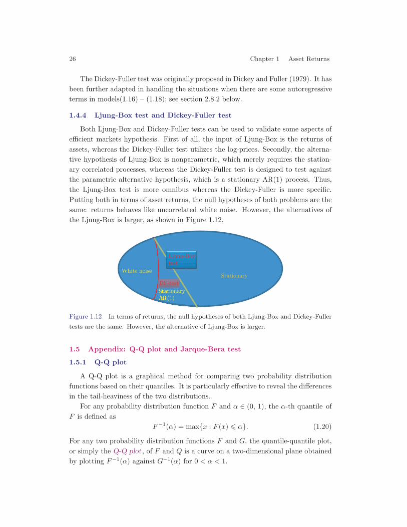
Both Ljung-Box and Dickey-Fuller tests can be used to validate some aspects ofefficient markets hypothesis. First of all, the input of Ljung-Box is the returns ofassets, whereas the Dickey-Fuller test utilizes the log-prices. Secondly, the alterna-tive hypothesis of Ljung-Box is nonparametric, which merely requires the station-ary correlated processes, whereas the Dickey-Fuller test is designed to test againstthe parametric alternative hypothesis, which is a stationary AR(1) process. Thus,the Ljung-Box test is more omnibus whereas the Dickey-Fuller is more specific.Putting both in terms of asset returns, the null hypotheses of both problems are thesame: returns behaves like uncorrelated white noise. However, the alternatives ofthe Ljung-Box is larger, as shown in Figure 1.12.

Figure 1.12 In terms of returns, the null hypotheses of both Ljung-Box and Dickey-Fuller

tests are the same. However, the alternative of Ljung-Box is larger.

1.5 Appendix: Q-Q plot and Jarque-Bera test

1.5.1 Q-Q plot

A Q-Q plot is a graphical method for comparing two probability distributionfunctions based on their quantiles. It is particularly effective to reveal the differencesin the tail-heaviness of the two distributions.

For any probability distribution function F and α ∈ (0, 1), the α-th quantile ofF is defined as

F−1(α) = max{x : F (x) � α}. (1.20)

For any two probability distribution functions F and G, the quantile-quantile plot,or simply the Q-Q plot , of F and Q is a curve on a two-dimensional plane obtainedby plotting F−1(α) against G−1(α) for 0 < α < 1.

1.5 Appendix: Q-Q plot and Jarque-Bera test 27

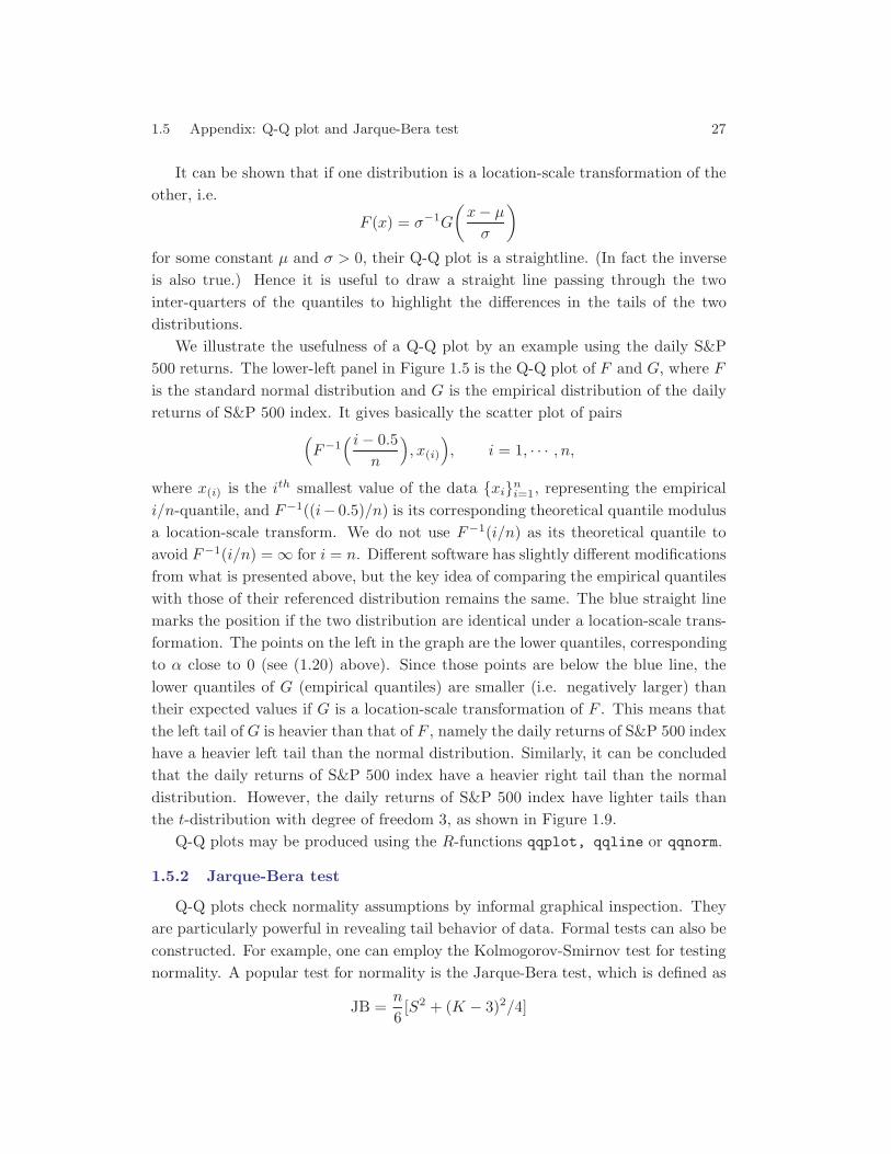
It can be shown that if one distribution is a location-scale transformation of theother, i.e.

F (x) = σ−1G(x− μ

σ

)for some constant μ and σ > 0, their Q-Q plot is a straightline. (In fact the inverseis also true.) Hence it is useful to draw a straight line passing through the twointer-quarters of the quantiles to highlight the differences in the tails of the twodistributions.

We illustrate the usefulness of a Q-Q plot by an example using the daily S&P500 returns. The lower-left panel in Figure 1.5 is the Q-Q plot of F and G, where Fis the standard normal distribution and G is the empirical distribution of the dailyreturns of S&P 500 index. It gives basically the scatter plot of pairs(

F−1( i− 0.5

n

), x(i)

), i = 1, · · · , n,

where x(i) is the ith smallest value of the data {xi}ni=1, representing the empiricali/n-quantile, and F−1((i− 0.5)/n) is its corresponding theoretical quantile modulusa location-scale transform. We do not use F−1(i/n) as its theoretical quantile toavoid F−1(i/n) =∞ for i = n. Different software has slightly different modificationsfrom what is presented above, but the key idea of comparing the empirical quantileswith those of their referenced distribution remains the same. The blue straight linemarks the position if the two distribution are identical under a location-scale trans-formation. The points on the left in the graph are the lower quantiles, correspondingto α close to 0 (see (1.20) above). Since those points are below the blue line, thelower quantiles of G (empirical quantiles) are smaller (i.e. negatively larger) thantheir expected values if G is a location-scale transformation of F . This means thatthe left tail of G is heavier than that of F , namely the daily returns of S&P 500 indexhave a heavier left tail than the normal distribution. Similarly, it can be concludedthat the daily returns of S&P 500 index have a heavier right tail than the normaldistribution. However, the daily returns of S&P 500 index have lighter tails thanthe t-distribution with degree of freedom 3, as shown in Figure 1.9.

Q-Q plots may be produced using the R-functions qqplot, qqline or qqnorm.

1.5.2 Jarque-Bera test

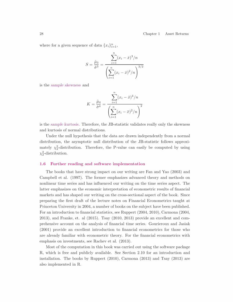
Q-Q plots check normality assumptions by informal graphical inspection. Theyare particularly powerful in revealing tail behavior of data. Formal tests can also beconstructed. For example, one can employ the Kolmogorov-Smirnov test for testingnormality. A popular test for normality is the Jarque-Bera test, which is defined as

JB =n

6[S2 + (K − 3)2/4]


where for a given sequence of data {xi}ni=1,

S =μ̂3σ̂3

=

n∑i=1

(xi − x̄)3/n

(n∑i=1

(xi − x̄)2/n

)3/2

is the sample skewness and

K =μ̂4σ̂4

=

n∑i=1

(xi − x̄)4/n(n∑i=1

(xi − x̄)2/n

)2

is the sample kurtosis. Therefore, the JB-statistic validates really only the skewnessand kurtosis of normal distributions.

Under the null hypothesis that the data are drawn independently from a normaldistribution, the asymptotic null distribution of the JB-statistic follows approxi-mately χ22-distribution. Therefore, the P-value can easily be computed by usingχ22-distribution.

1.6 Further reading and software implementation

The books that have strong impact on our writing are Fan and Yao (2003) andCampbell et al. (1997). The former emphasizes advanced theory and methods onnonlinear time series and has influenced our writing on the time series aspect. Thelatter emphasizes on the economic interpretation of econometric results of financialmarkets and has shaped our writing on the cross-sectional aspect of the book. Sincepreparing the first draft of the lecture notes on Financial Econometrics taught atPrinceton University in 2004, a number of books on the subject have been published.For an introduction to financial statistics, see Ruppert (2004, 2010), Carmona (2004,2013), and Franke, et. al (2015). Tsay (2010, 2013) provide an excellent and com-prehensive account on the analysis of financial time series. Gourieroux and Jasiak(2001) provide an excellent introduction to financial econometrics for those whoare already familiar with econometric theory. For the financial econometrics withemphasis on investments, see Rachev et al. (2013).

Most of the computation in this book was carried out using the software packageR, which is free and publicly available. See Section 2.10 for an introduction andinstallation. The books by Ruppert (2010), Carmona (2013) and Tsay (2013) arealso implemented in R.

1.7 Exercises 29

It is our hope that readers will be stimulated to use the methods described inthis book for their own applications and research. Our aim is to provide informationin sufficient detail so that readers can produce their own implementations. This willbe a valuable exercise for students and readers who are new to the area. To assistthis endeavor, we have placed all of the data sets and codes used in this book on thefollowing web site:

http://orfe.princeton.edu/~jqfan/fan/FinEcon.html

1.7 Exercises

1.1 Download the daily, weekly and monthly prices for the Nasdaq index and the IBM

stock from Yahoo!Finance. Reproduce Figures 1.3 – 1.8 using the Nasdaq index and

the IBM stock data instead.

1.2 Consider a path dependent payoff function Yt = a1rt+1 + · · · + akrt+k where {ai}ki=1

are given weights. If the return time series is weak stationary in the sense that

cov(rt, rt+j) = γ(j). Show that

var(Yt) =

k∑i=1

k∑j=1

aiajγi−j .

A natural estimate of this variance is the following substitution estimator:

v̂ar(Yt) =k∑

i=1

k∑j=1

aiaj γ̂i−j ,

where γ̂i−j is defined by (1.8). Show that v̂ar(Yt) � 0.

1.3 Consider the following quote from Eugene Fama who was Myron Scholes’ thesis adviser:

If the population of prices changes is strictly normal, on the average for any stock · · ·an observation more than five standard deviations from the mean should be observed

about once every 7000 years. In fact such observations seem to occur about once every

three or four years.

(See Lowenstein, 2001, page 71.) For X ∼ N(μ, σ2), P (|X − μ| > 5σ) = 5.733 × 10−7,

deduce how many observations per year Fama was implicitly assuming to be made. If

a year is defined as 252 trading days and daily returns are normal, how many years is

it expected to take to get a 5 standard deviation event? How does the answer to the

last question change when the daily returns follow the t-distribution with 4 degrees of

freedom.

1.4 Is the (marginal) distribution of log-returns over a long time horizon (e.g. monthly or

quarterly) close to normal? Explain briefly.

1.5 Generate a random sample of size 1000 from the t-distribution with ν degrees of freedom

and another random sample of size 1000 from the standard normal distribution. Apply

the Kolmogorov-Smirnov test to check if they come from the same distribution. Report

the results for ν = 5, 10, 15 and 20.


1.6 Report the P-values for appying the Jarque-Bera test to the data given in Exercise 1.1.

What can you conclude based on these P-values?

1.7 Generate a random sample of size 100 from the t-distribution with ν degrees of freedom

for ν = 5, 15 and ∞ (i.e. normal distribution). Apply the Jarque-Bera test to check

the normality and report the P-values.

1.8 According to the efficient market hypothesis, is the return of a portfolio predictable?

Is the volatility of a portfolio predictable? State the most appropriate mathematical

form of the efficient market hypothesis.

1.9 If the Ljung-Box test is employed to test the efficient market hypothesis, what null

hypothesis is to be tested? If the autocorrelation for the first 4 lags of the monthly

log-returns of the S&P 500 is

ρ̂(1) = 0.2, ρ̂(2) = −0.15, ρ̂(3) = 0.25, ρ̂(4) = 0.12

based on past 5 years data, is the efficient market hypothesis reasonable?

1.10 Generate 400 time series from the independent Gaussian white noise {rt}Tt=1 with

T = 100. Compute

Z =√T ρ̂(1), Qm, Q∗

m

for m = 3, 6, and 12. Plot the histograms of Z, Q3, Q∗3 and Q6 and compare it

with their asymptotic distributions. Report the first, fifth and tenth percentiles of the

statistic |Z1|, Q3, Q∗3, Q6, Q

∗6, Q12 and Q∗

12, among 400 simulations and compare them

with their theoretical (asymptotic) percentiles.

1.11 Repeat the experiment in Exercise 1.10 when T = 400 and rt is generated from the

t-distribution with degree of freedom 5.

1.12 What is the alternative hypothesis of the Dickey-Fuller test for the random walk?

Suppose that based on last 120 quarterly data on the US GDP, it was computed that

α̂ = 0.95. Does the US GDP follow a random walk with a drift? Answer the question

at 5% significance level (the critical value is -13.96) using the Dickey-Fuller coefficient

test for the model with drift.

1.13 (Implication of martingale hypothesis). Let St be the price of an asset at time t. One

version of the EMH assumes that the prices of any asset form a martingale process in

the sense that

E(St+1|St, St−1, · · · ) = St, for all t.

To understand the implication of this assumption, we consider the following simple

investment strategy. With initial capital C0 dollars, at the time t we hold αt dollars

in cash and βt shares of an asset at the price St. Hence the value of our investment

at time t is Ct = αt + βtSt. Suppose that our investment is self-financing in the sense

that

Ct+1 = αt + βtSt+1 = αt+1 + βt+1St+1,

and our investment strategy (αt+1, βt+1) is entirely determined by the asset prices up

to the time t. Show that if {St} is a martingale process, there exist no strategies such

that Ct+1 > Ct with probability 1.

Chapter 2

Linear Time Series Models

Data obtained from observations collected sequentially over time are common inthis information age. For example, we have collections on daily stock prices, weeklyinterest rates, monthly sales figures, quarterly consumer price indices (CPI) andannual gross domestic product (GDP) figures. Those data collected over time arecalled time series. The purpose of analyzing time series data is in general two-fold:to understand the stochastic mechanism that generates the data, and to predictor forecast the future values of a time series. This chapter introduces a class oflinear time series models, or more precisely, a class of models which depict thelinear features (including linear dependence) of time series. Those linear modelsand associated inference techniques provide the basic framework for the study of thelinear dynamic structure of financial time series and for forecasting future valuesbased on linear dependence structures.

2.1 Stationarity

One of the important aspects of time series analysis is to use the data collectedin the past to forecast the future. How can historical data be useful for forecastinga future event? This is through the assumption of stationarity which refers to sometime-invariance properties of the underlying process. For example, we may assumethat the correlation between the returns of tomorrow and today is the same asthose between any two successive days in the past. This enables us to aggregate theinformation from the data in the past to learn about the correlation. This correlationinvariance over time is a typical characteristic of the so called weak stationarity orcovariance stationarity . It facilitates linear prediction which is essentially basedon the correlation between a predicated variable and its predictor (such as in linearregression). A stronger time-invariant assumption is that the joint distribution of thereturns in a week in the future is the same as that in any weeks in the past. In otherwords, prediction is always based on some invariance properties over time, althoughthe invariance may refer to some characteristics of the probability distribution ofthe process, or to the law governing the change of the distribution. We introducethe concept of stationarity more formally below.

32 Chapter 2 Linear Time Series Models

A sequence of random variables {Xt, t = 0,±1,±2, · · · } is called a stochastic pro-cess and is served as a model for a set of observed time series data. It is convenientto refer to {Xt} itself as a time series. It is known that the complete probabilitystructure of {Xt} is determined by the set of all the finite-dimensional distributionsof {Xt}. Fortunately most linear features concerned depend on the first two mo-ments of {Xt}, which are the main objects depicted in linear time series models.Of course if {Xt} is a Gaussian process in the sense that all its finite-dimensionaldistributions are normal, the first two moments then determine the the probabilitystructure of {Xt} completely and {Xt} is a linear process.

A time series {Xt} is said to be weakly stationary (or second order stationary orcovariance stationary ) if E(X2

t ) < ∞ and both EXt and cov(Xt, Xt+k), for anyinteger k, do not depend on t.

For weakly stationary time series {Xt}, let μ = EXt denote its common mean.We define the autocovariance function (ACVF) as

γ(k) = cov(Xt, Xt+k) = E{(Xt − μ)(Xt+k − μ)}, (2.1)

and the autocorrelation function (ACF) as

ρ(k) = Corr(Xt, Xt+k) = γ(k)/γ(0) (2.2)

for k = 0,±1,±2, · · · . Note that γ(0) = var(Xt) is independent of t. For simplicity,we drop the adverb “weakly” and call {Xt} stationary if it is weakly stationary, i.e.{Xt} has finite and time-invariant first two moments. It is easy to see that ρ(0) = 1and ρ(k) = ρ(−k) for any stationary processes, and that the variance-covariancematrix of the vector (Xt, · · · , Xt+k) is

var(Xt, · · · , Xt+k) =

⎛⎜⎜⎜⎜⎝γ(0) γ(1) γ(2) · · · γ(k − 1)γ(1) γ(0) γ(1) · · · γ(k − 2)...

......

...γ(k − 2) γ(k − 3) γ(k − 4) · · · γ(1)γ(k − 1) γ(k − 2) γ(k − 3) · · · γ(0)

⎞⎟⎟⎟⎟⎠ .

Therefore, for any linear combinations,

var(k∑

i=1

aiXt+i)=k∑

i=1

k∑j=1

aiajcov(Xt+i, Xt+k)

=k∑

i=1

k∑j=1

aiajγ(i− j) � 0. (2.3)

2.2 Stationary ARMA models 33

As such, the function γ(·) is referred to as the semi-positive definite function.

A very specific class of processes that plays a similar role to zero in the numbertheory is the white noise. When ρ(k) = 0 for any k = 0, {Xt} is called a white noise,and is denoted by Xt ∼ WN(μ, σ2), where σ2 = γ(0) = var(Xt). In other words,a white noise is a sequence of uncorrelated random variables with the same meanand the same variance. White noise processes are building blocks for constructinggeneral stationary processes.

In practice we use an observed sample X1, · · · , XT to estimate ACVF and ACFby the sample ACVF and sample ACF . They are basically the sample covarianceand sample correlation of the lagged pairs {(Xt−k, Xk)}Tt=k+1. Formally, they aredefined as follows

γ̂(k) =1T

T∑t=k+1

(Xt − X̄)(Xt−k − X̄), ρ̂(k) = γ̂(k)/γ̂(0), (2.4)

where X̄ = T−1∑

1�t�T Xt. In the estimator γ̂(k), we use the divisor T insteadof T − k. This is a common practice adopted by almost all statistical packages.It ensures that the function γ̂(·) is semi-positive definite (Exercise 2.2), a propertygiven by (2.3). See Fan and Yao (2003) pp.42 for further discussion on this choice.

Weak stationarity is indeed a very weak notion of stationarity. For example, if{Xt} is weakly stationary, it does not imply that {X2

t } is weakly stationary. Yet, thelatter time series has very strong connections with the volatility of financial returns.Therefore, we need a stronger version of stationarity as follows.

A time series {Xt, t = 0,±1,±2, · · · } is said to be strongly stationary or strictly

stationary if the k-dimensional distribution of (X1, · · · , Xk) is the same as that of(Xt+1, · · · , Xt+k) for any k � 1 and t.

This assumption is needed in the context of nonlinear prediction. Obviously thestrict stationarity implies the (weak) stationarity provided E(X2

t ) <∞. In addition,the strong stationarity of {Xt, t = 0,±1,±2, · · · } implies that of the time series{g(Xt), t = 0,±1,±2, · · · } is also strongly stationary for any function g.

2.2 Stationary ARMA models

One of the most frequently used time series models is the stationary autoregres-

sive moving average (ARMA) model. It is frequently used in modeling the dynamicson returns of financial assets and other time series.

34 Chapter 2 Linear Time Series Models

2.2.1 Moving average processes

Perhaps the simplest stationary time series are moving average (MA) processes.They also facilitate the computation of the autocovariance function easily. A simpleexample of this is the k-period return (1.6).

Let εt ∼ WN(0, σ2). For a fixed integer q � 1, we write Xt ∼ MA(q) if Xt isdefined as a moving average of q successive εt as follows:

Xt = μ+ εt + a1εt−1 + · · ·+ aqεt−q, (2.5)

where μ, a1, · · · , aq are constant coefficients. In the above definition, εt stands forthe innovation at time t, and the innovations εt, εt−1, · · · are unobservable. Theintuition behind the moving average equation (2.5) may be understood as follows:innovation εt stands for the shock to the market at time t and Xt is the impact onthe return from the innovations up to time t. The coefficient ak is regarded as a“discount” factor on the k-lagged innovation εt−k. For example, for ak = bk and|b| < 1, the impact of εt fades away exponentially over time.

In fact Xt defined by (2.5) is always stationary with EXt = μ, as the coefficientsa1, · · · , aq do not vary over time. We first use a simple example to illustrate how tocalculate ACVF and ACF for MA processes.

Example 2.1 For MA(1) model Xt = μ+ εt + aεt−1, it holds

γ(0) = var(Xt) = var(εt) + var(aεt−1) + 2cov(εt, aεt−1) = (1 + a2)σ2.

Similarly,

γ(1) = cov(Xt, Xt−1) = cov(εt + aεt−1, εt−1 + aεt−2) = aσ2,

since there is only one common term, εt−1 in both Xt and Xt−1. Now for the ACVFof lag two, we have

Xt = μ+ εt + aεt−1,

which does not share the same set of innovations {εt} as

Xt−2 = μ+ εt−2 + aεt−3.

Therefore γ(2) = 0. Similarly, γ(k) = 0 for any k � 2. Consequently,

ρ(1) = a/(1 + a2), ρ(k) = 0 for any |k| > 1. (2.6)

Since 2|a| < 1 + a2, |ρ(1)| � 0.5 for any MA(1) process.

chapter 1 asset returns - princeton universityorfe.princeton.edu/~jqfan/fan/finecon/chap1.pdf ·...

Documents