chap5 basic association analysis - university of minnesota
TRANSCRIPT

3/8/2021 Introduction to Data Mining, 2nd Edition 1
Data Mining
Chapter 5
Association Analysis: Basic Concepts
Introduction to Data Mining, 2nd Edition
by
Tan, Steinbach, Karpatne, Kumar
3/8/2021 Introduction to Data Mining, 2nd Edition 2
Association Rule Mining
Given a set of transactions, find rules that will predict the occurrence of an item based on the occurrences of other items in the transaction
Market-Basket transactions
TID Items
1 Bread, Milk
2 Bread, Diaper, Beer, Eggs
3 Milk, Diaper, Beer, Coke
4 Bread, Milk, Diaper, Beer
5 Bread, Milk, Diaper, Coke
Example of Association Rules
{Diaper} {Beer},{Milk, Bread} {Eggs,Coke},{Beer, Bread} {Milk},
Implication means co-occurrence, not causality!
1
2

3/8/2021 Introduction to Data Mining, 2nd Edition 3
Definition: Frequent Itemset
Itemset
– A collection of one or more items
Example: {Milk, Bread, Diaper}
– k-itemset
An itemset that contains k items
Support count ()
– Frequency of occurrence of an itemset
– E.g. ({Milk, Bread,Diaper}) = 2
Support
– Fraction of transactions that contain an itemset
– E.g. s({Milk, Bread, Diaper}) = 2/5
Frequent Itemset
– An itemset whose support is greater than or equal to a minsup threshold
TID Items
1 Bread, Milk
2 Bread, Diaper, Beer, Eggs
3 Milk, Diaper, Beer, Coke
4 Bread, Milk, Diaper, Beer
5 Bread, Milk, Diaper, Coke
3/8/2021 Introduction to Data Mining, 2nd Edition 4
Definition: Association Rule
Example:Beer}{}Diaper,Milk{
4.052
|T|)BeerDiaper,,Milk(
s
67.032
)Diaper,Milk()BeerDiaper,Milk,(
c
Association Rule
– An implication expression of the form X Y, where X and Y are itemsets
– Example:{Milk, Diaper} {Beer}
Rule Evaluation Metrics
– Support (s)
Fraction of transactions that contain both X and Y
– Confidence (c)
Measures how often items in Y appear in transactions thatcontain X
TID Items
1 Bread, Milk
2 Bread, Diaper, Beer, Eggs
3 Milk, Diaper, Beer, Coke
4 Bread, Milk, Diaper, Beer
5 Bread, Milk, Diaper, Coke
3
4

3/8/2021 Introduction to Data Mining, 2nd Edition 5
Association Rule Mining Task
Given a set of transactions T, the goal of association rule mining is to find all rules having – support ≥ minsup threshold
– confidence ≥ minconf threshold
Brute-force approach:– List all possible association rules
– Compute the support and confidence for each rule
– Prune rules that fail the minsup and minconfthresholds
Computationally prohibitive!
3/8/2021 Introduction to Data Mining, 2nd Edition 6
Computational Complexity
Given d unique items:– Total number of itemsets = 2d
– Total number of possible association rules:
123 1
1
1 1
dd
d
k
kd
j j
kd
k
dR
If d=6, R = 602 rules
5
6

3/8/2021 Introduction to Data Mining, 2nd Edition 7
Mining Association Rules
Example of Rules:
{Milk,Diaper} {Beer} (s=0.4, c=0.67){Milk,Beer} {Diaper} (s=0.4, c=1.0){Diaper,Beer} {Milk} (s=0.4, c=0.67){Beer} {Milk,Diaper} (s=0.4, c=0.67) {Diaper} {Milk,Beer} (s=0.4, c=0.5) {Milk} {Diaper,Beer} (s=0.4, c=0.5)
TID Items
1 Bread, Milk
2 Bread, Diaper, Beer, Eggs
3 Milk, Diaper, Beer, Coke
4 Bread, Milk, Diaper, Beer
5 Bread, Milk, Diaper, Coke
Observations:
• All the above rules are binary partitions of the same itemset: {Milk, Diaper, Beer}
• Rules originating from the same itemset have identical support butcan have different confidence
• Thus, we may decouple the support and confidence requirements
3/8/2021 Introduction to Data Mining, 2nd Edition 8
Mining Association Rules
Two-step approach: 1. Frequent Itemset Generation
– Generate all itemsets whose support minsup
2. Rule Generation– Generate high confidence rules from each frequent itemset,
where each rule is a binary partitioning of a frequent itemset
Frequent itemset generation is still computationally expensive
7
8
3/8/2021 Introduction to Data Mining, 2nd Edition 9
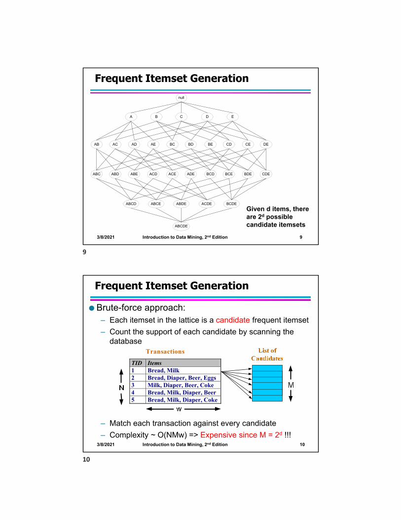
Frequent Itemset Generationnull
AB AC AD AE BC BD BE CD CE DE
A B C D E
ABC ABD ABE ACD ACE ADE BCD BCE BDE CDE
ABCD ABCE ABDE ACDE BCDE
ABCDE
Given d items, there are 2d possible candidate itemsets
3/8/2021 Introduction to Data Mining, 2nd Edition 10
Frequent Itemset Generation
Brute-force approach: – Each itemset in the lattice is a candidate frequent itemset
– Count the support of each candidate by scanning the database
– Match each transaction against every candidate
– Complexity ~ O(NMw) => Expensive since M = 2d !!!
TID Items 1 Bread, Milk 2 Bread, Diaper, Beer, Eggs 3 Milk, Diaper, Beer, Coke 4 Bread, Milk, Diaper, Beer 5 Bread, Milk, Diaper, Coke
Transactions
9
10
3/8/2021 Introduction to Data Mining, 2nd Edition 11
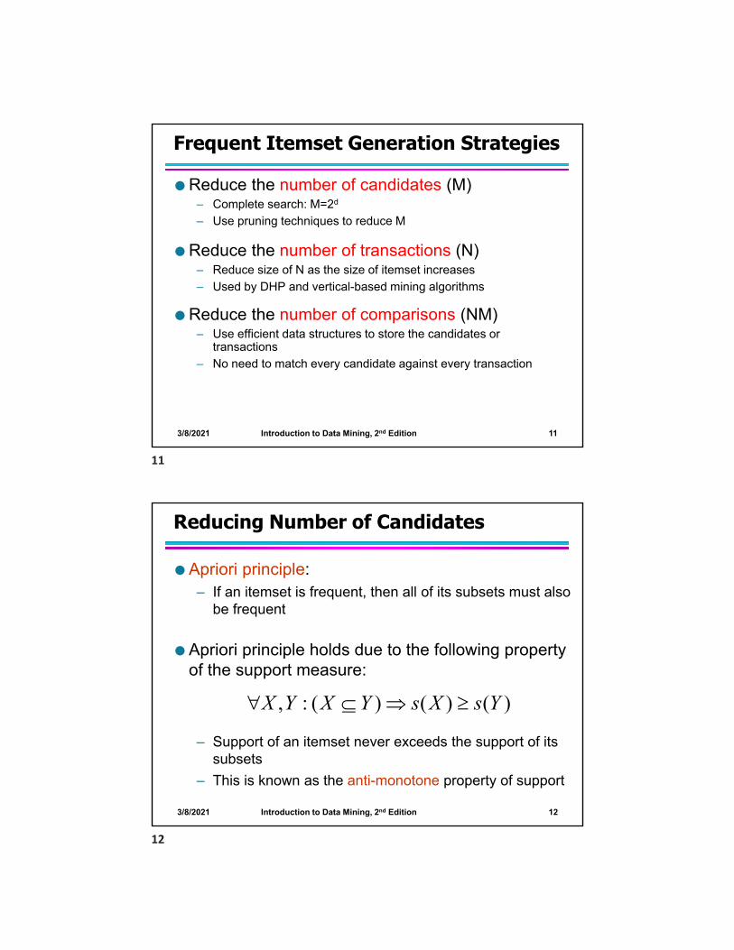
Frequent Itemset Generation Strategies
Reduce the number of candidates (M)– Complete search: M=2d
– Use pruning techniques to reduce M
Reduce the number of transactions (N)– Reduce size of N as the size of itemset increases
– Used by DHP and vertical-based mining algorithms
Reduce the number of comparisons (NM)– Use efficient data structures to store the candidates or
transactions
– No need to match every candidate against every transaction
3/8/2021 Introduction to Data Mining, 2nd Edition 12
Reducing Number of Candidates
Apriori principle:– If an itemset is frequent, then all of its subsets must also
be frequent
Apriori principle holds due to the following property of the support measure:
– Support of an itemset never exceeds the support of its subsets
– This is known as the anti-monotone property of support
)()()(:, YsXsYXYX
11
12

3/8/2021 Introduction to Data Mining, 2nd Edition 13
Found to be Infrequent
Illustrating Apriori Principle
Pruned supersets
3/8/2021 Introduction to Data Mining, 2nd Edition 14
Illustrating Apriori Principle
Minimum Support = 3
TID Items
1 Bread, Milk
2 Beer, Bread, Diaper, Eggs
3 Beer, Coke, Diaper, Milk
4 Beer, Bread, Diaper, Milk
5 Bread, Coke, Diaper, Milk
Items (1-itemsets)
If every subset is considered, 6C1 + 6C2 + 6C36 + 15 + 20 = 41
With support-based pruning,6 + 6 + 4 = 16
Item Count Bread 4 Coke 2 Milk 4 Beer 3 Diaper 4 Eggs 1
TID Items
1 Bread, Milk
2 Beer, Bread, Diaper, Eggs
3 Beer, Coke, Diaper, Milk
4 Beer, Bread, Diaper, Milk
5 Bread, Coke, Diaper, Milk
13
14

3/8/2021 Introduction to Data Mining, 2nd Edition 15
Illustrating Apriori Principle
Minimum Support = 3
If every subset is considered, 6C1 + 6C2 + 6C36 + 15 + 20 = 41
With support-based pruning,6 + 6 + 4 = 16
TID Items
1 Bread, Milk
2 Beer, Bread, Diaper, Eggs
3 Beer, Coke, Diaper, Milk
4 Beer, Bread, Diaper, Milk
5 Bread, Coke, Diaper, Milk
Items (1-itemsets)
Item Count Bread 4 Coke 2 Milk 4 Beer 3 Diaper 4 Eggs 1
3/8/2021 Introduction to Data Mining, 2nd Edition 16
Illustrating Apriori Principle
Item Count Bread 4 Coke 2 Milk 4 Beer 3 Diaper 4 Eggs 1
Itemset {Bread,Milk} {Bread, Beer } {Bread,Diaper} {Beer, Milk} {Diaper, Milk} {Beer,Diaper}
Items (1-itemsets)
Pairs (2-itemsets)
(No need to generatecandidates involving Cokeor Eggs)
Minimum Support = 3
If every subset is considered, 6C1 + 6C2 + 6C36 + 15 + 20 = 41
With support-based pruning,6 + 6 + 4 = 16
TID Items
1 Bread, Milk
2 Beer, Bread, Diaper, Eggs
3 Beer, Coke, Diaper, Milk
4 Beer, Bread, Diaper, Milk
5 Bread, Coke, Diaper, Milk
15
16

3/8/2021 Introduction to Data Mining, 2nd Edition 17
Illustrating Apriori Principle
Item Count Bread 4 Coke 2 Milk 4 Beer 3 Diaper 4 Eggs 1
Itemset Count {Bread,Milk} 3 {Beer, Bread} 2 {Bread,Diaper} 3 {Beer,Milk} 2 {Diaper,Milk} 3 {Beer,Diaper} 3
Items (1-itemsets)
Pairs (2-itemsets)
(No need to generatecandidates involving Cokeor Eggs)
Minimum Support = 3
If every subset is considered, 6C1 + 6C2 + 6C36 + 15 + 20 = 41
With support-based pruning,6 + 6 + 4 = 16
TID Items
1 Bread, Milk
2 Beer, Bread, Diaper, Eggs
3 Beer, Coke, Diaper, Milk
4 Beer, Bread, Diaper, Milk
5 Bread, Coke, Diaper, Milk
3/8/2021 Introduction to Data Mining, 2nd Edition 18
Illustrating Apriori Principle
Item Count Bread 4 Coke 2 Milk 4 Beer 3 Diaper 4 Eggs 1
Itemset Count {Bread,Milk} 3 {Bread,Beer} 2 {Bread,Diaper} 3 {Milk,Beer} 2 {Milk,Diaper} 3 {Beer,Diaper} 3
Itemset { Beer, Diaper, Milk} { Beer,Bread,Diaper} {Bread,Diaper,Milk} { Beer, Bread, Milk}
Items (1-itemsets)
Pairs (2-itemsets)
(No need to generatecandidates involving Cokeor Eggs)
Triplets (3-itemsets)Minimum Support = 3
If every subset is considered, 6C1 + 6C2 + 6C36 + 15 + 20 = 41
With support-based pruning,6 + 6 + 4 = 16
If every subset is considered, 6C1 + 6C2 + 6C36 + 15 + 20 = 41
With support-based pruning,6 + 6 + 4 = 16
TID Items
1 Bread, Milk
2 Beer, Bread, Diaper, Eggs
3 Beer, Coke, Diaper, Milk
4 Beer, Bread, Diaper, Milk
5 Bread, Coke, Diaper, Milk
17
18

3/8/2021 Introduction to Data Mining, 2nd Edition 19
Illustrating Apriori Principle
Item Count Bread 4 Coke 2 Milk 4 Beer 3 Diaper 4 Eggs 1
Itemset Count {Bread,Milk} 3 {Bread,Beer} 2 {Bread,Diaper} 3 {Milk,Beer} 2 {Milk,Diaper} 3 {Beer,Diaper} 3
Itemset Count { Beer, Diaper, Milk} { Beer,Bread, Diaper} {Bread, Diaper, Milk} {Beer, Bread, Milk}
2 2 2 1
Items (1-itemsets)
Pairs (2-itemsets)
(No need to generatecandidates involving Cokeor Eggs)
Triplets (3-itemsets)Minimum Support = 3
If every subset is considered, 6C1 + 6C2 + 6C36 + 15 + 20 = 41
With support-based pruning,6 + 6 + 4 = 16
TID Items
1 Bread, Milk
2 Beer, Bread, Diaper, Eggs
3 Beer, Coke, Diaper, Milk
4 Beer, Bread, Diaper, Milk
5 Bread, Coke, Diaper, Milk
3/8/2021 Introduction to Data Mining, 2nd Edition 20
Illustrating Apriori Principle
Item Count Bread 4 Coke 2 Milk 4 Beer 3 Diaper 4 Eggs 1
Itemset Count {Bread,Milk} 3 {Bread,Beer} 2 {Bread,Diaper} 3 {Milk,Beer} 2 {Milk,Diaper} 3 {Beer,Diaper} 3
Itemset Count { Beer, Diaper, Milk} { Beer,Bread, Diaper} {Bread, Diaper, Milk} {Beer, Bread, Milk}
2 2 2 1
Items (1-itemsets)
Pairs (2-itemsets)
(No need to generatecandidates involving Cokeor Eggs)
Triplets (3-itemsets)Minimum Support = 3
If every subset is considered, 6C1 + 6C2 + 6C36 + 15 + 20 = 41
With support-based pruning,6 + 6 + 4 = 166 + 6 + 1 = 13
TID Items
1 Bread, Milk
2 Beer, Bread, Diaper, Eggs
3 Beer, Coke, Diaper, Milk
4 Beer, Bread, Diaper, Milk
5 Bread, Coke, Diaper, Milk
19
20

3/8/2021 Introduction to Data Mining, 2nd Edition 21
Apriori Algorithm
– Fk: frequent k-itemsets– Lk: candidate k-itemsets
Algorithm– Let k=1– Generate F1 = {frequent 1-itemsets}– Repeat until Fk is empty
Candidate Generation: Generate Lk+1 from Fk
Candidate Pruning: Prune candidate itemsets in Lk+1 containing subsets of length k that are infrequent
Support Counting: Count the support of each candidate in Lk+1 by scanning the DB
Candidate Elimination: Eliminate candidates in Lk+1 that are infrequent, leaving only those that are frequent => Fk+1
3/8/2021 Introduction to Data Mining, 2nd Edition 22
Candidate Generation: Brute-force method
TID Items
1 Bread, Milk
2 Beer, Bread, Diaper, Eggs
3 Beer, Coke, Diaper, Milk
4 Beer, Bread, Diaper, Milk
5 Bread, Coke, Diaper, Milk
21
22

3/8/2021 Introduction to Data Mining, 2nd Edition 23
Candidate Generation: Merge Fk-1 and F1 itemsets
3/8/2021 Introduction to Data Mining, 2nd Edition 24
Candidate Generation: Fk-1 x Fk-1 Method
Merge two frequent (k-1)-itemsets if their first (k-2) items are identical
F3 = {ABC,ABD,ABE,ACD,BCD,BDE,CDE}– Merge(ABC, ABD) = ABCD
– Merge(ABC, ABE) = ABCE
– Merge(ABD, ABE) = ABDE
– Do not merge(ABD,ACD) because they share only prefix of length 1 instead of length 2
23
24

3/8/2021 Introduction to Data Mining, 2nd Edition 25
Candidate Pruning
Let F3 = {ABC,ABD,ABE,ACD,BCD,BDE,CDE} be the set of frequent 3-itemsets
L4 = {ABCD,ABCE,ABDE} is the set of candidate 4-itemsets generated (from previous slide)
Candidate pruning– Prune ABCE because ACE and BCE are infrequent
– Prune ABDE because ADE is infrequent
After candidate pruning: L4 = {ABCD}
3/8/2021 Introduction to Data Mining, 2nd Edition 26
Candidate Generation: Fk-1 x Fk-1 Method
25
26

3/8/2021 Introduction to Data Mining, 2nd Edition 27
Illustrating Apriori Principle
Item Count Bread 4 Coke 2 Milk 4 Beer 3 Diaper 4 Eggs 1
Itemset Count {Bread,Milk} 3 {Bread,Beer} 2 {Bread,Diaper} 3 {Milk,Beer} 2 {Milk,Diaper} 3 {Beer,Diaper} 3
Itemset Count {Bread, Diaper, Milk}
2
Items (1-itemsets)
Pairs (2-itemsets)
(No need to generatecandidates involving Cokeor Eggs)
Triplets (3-itemsets)Minimum Support = 3
If every subset is considered, 6C1 + 6C2 + 6C36 + 15 + 20 = 41
With support-based pruning,6 + 6 + 1 = 13 Use of Fk-1xFk-1 method for candidate generation results in
only one 3-itemset. This is eliminated after the support counting step.
3/8/2021 Introduction to Data Mining, 2nd Edition 28
Alternate Fk-1 x Fk-1 Method
Merge two frequent (k-1)-itemsets if the last (k-2) items of the first one is identical to the first (k-2) items of the second.
F3 = {ABC,ABD,ABE,ACD,BCD,BDE,CDE}– Merge(ABC, BCD) = ABCD
– Merge(ABD, BDE) = ABDE
– Merge(ACD, CDE) = ACDE
– Merge(BCD, CDE) = BCDE
27
28

3/8/2021 Introduction to Data Mining, 2nd Edition 29
Candidate Pruning for Alternate Fk-1 x Fk-1 Method
Let F3 = {ABC,ABD,ABE,ACD,BCD,BDE,CDE} be the set of frequent 3-itemsets
L4 = {ABCD,ABDE,ACDE,BCDE} is the set of candidate 4-itemsets generated (from previous slide)
Candidate pruning– Prune ABDE because ADE is infrequent
– Prune ACDE because ACE and ADE are infrequent
– Prune BCDE because BCE
After candidate pruning: L4 = {ABCD}
3/8/2021 Introduction to Data Mining, 2nd Edition 30
Support Counting of Candidate Itemsets
Scan the database of transactions to determine the support of each candidate itemset
– Must match every candidate itemset against every transaction, which is an expensive operation
TID Items
1 Bread, Milk
2 Beer, Bread, Diaper, Eggs
3 Beer, Coke, Diaper, Milk
4 Beer, Bread, Diaper, Milk
5 Bread, Coke, Diaper, Milk
Itemset { Beer, Diaper, Milk} { Beer,Bread,Diaper} {Bread, Diaper, Milk} { Beer, Bread, Milk}
29
30

3/8/2021 Introduction to Data Mining, 2nd Edition 31
Support Counting of Candidate Itemsets
To reduce number of comparisons, store the candidate itemsets in a hash structure
– Instead of matching each transaction against every candidate, match it against candidates contained in the hashed buckets
TID Items 1 Bread, Milk 2 Bread, Diaper, Beer, Eggs 3 Milk, Diaper, Beer, Coke 4 Bread, Milk, Diaper, Beer 5 Bread, Milk, Diaper, Coke
Transactions
3/8/2021 Introduction to Data Mining, 2nd Edition 32
Support Counting: An Example
Suppose you have 15 candidate itemsets of length 3:
{1 4 5}, {1 2 4}, {4 5 7}, {1 2 5}, {4 5 8}, {1 5 9}, {1 3 6}, {2 3 4}, {5 6 7}, {3 4 5}, {3 5 6}, {3 5 7}, {6 8 9}, {3 6 7}, {3 6 8}
How many of these itemsets are supported by transaction (1,2,3,5,6)?
31
32

3/8/2021 Introduction to Data Mining, 2nd Edition 33
Support Counting Using a Hash Tree
2 3 45 6 7
1 4 51 3 6
1 2 44 5 7 1 2 5
4 5 81 5 9
3 4 5 3 5 63 5 76 8 9
3 6 73 6 8
1,4,7
2,5,8
3,6,9Hash function
Suppose you have 15 candidate itemsets of length 3:
{1 4 5}, {1 2 4}, {4 5 7}, {1 2 5}, {4 5 8}, {1 5 9}, {1 3 6}, {2 3 4}, {5 6 7}, {3 4 5}, {3 5 6}, {3 5 7}, {6 8 9}, {3 6 7}, {3 6 8}
You need:
• Hash function
• Max leaf size: max number of itemsets stored in a leaf node (if number of candidate itemsets exceeds max leaf size, split the node)
3/8/2021 Introduction to Data Mining, 2nd Edition 34
Support Counting Using a Hash Tree
1 5 9
1 4 5 1 3 63 4 5 3 6 7
3 6 8
3 5 6
3 5 7
6 8 9
2 3 4
5 6 7
1 2 4
4 5 71 2 5
4 5 8
1,4,7
2,5,8
3,6,9
Hash Function Candidate Hash Tree
Hash on 1, 4 or 7
33
34

3/8/2021 Introduction to Data Mining, 2nd Edition 35
Support Counting Using a Hash Tree
1 5 9
1 4 5 1 3 63 4 5 3 6 7
3 6 8
3 5 6
3 5 7
6 8 9
2 3 4
5 6 7
1 2 4
4 5 71 2 5
4 5 8
1,4,7
2,5,8
3,6,9
Hash Function Candidate Hash Tree
Hash on 2, 5 or 8
3/8/2021 Introduction to Data Mining, 2nd Edition 36
Support Counting Using a Hash Tree
1 5 9
1 4 5 1 3 63 4 5 3 6 7
3 6 8
3 5 6
3 5 7
6 8 9
2 3 4
5 6 7
1 2 4
4 5 71 2 5
4 5 8
1,4,7
2,5,8
3,6,9
Hash Function Candidate Hash Tree
Hash on 3, 6 or 9
35
36

3/8/2021 Introduction to Data Mining, 2nd Edition 37
Support Counting Using a Hash Tree
1 5 9
1 4 5 1 3 63 4 5 3 6 7
3 6 8
3 5 6
3 5 7
6 8 9
2 3 4
5 6 7
1 2 4
4 5 71 2 5
4 5 8
1 2 3 5 6
1 + 2 3 5 63 5 62 +
5 63 +
1,4,7
2,5,8
3,6,9
Hash Functiontransaction
3/8/2021 Introduction to Data Mining, 2nd Edition 38
Support Counting Using a Hash Tree
1 5 9
1 4 5 1 3 63 4 5 3 6 7
3 6 8
3 5 6
3 5 7
6 8 9
2 3 4
5 6 7
1 2 4
4 5 71 2 5
4 5 8
1,4,7
2,5,8
3,6,9
Hash Function1 2 3 5 6
3 5 61 2 +
5 61 3 +
61 5 +
3 5 62 +
5 63 +
1 + 2 3 5 6
transaction
37
38

3/8/2021 Introduction to Data Mining, 2nd Edition 39
Support Counting Using a Hash Tree
1 5 9
1 4 5 1 3 63 4 5 3 6 7
3 6 8
3 5 6
3 5 7
6 8 9
2 3 4
5 6 7
1 2 4
4 5 71 2 5
4 5 8
1,4,7
2,5,8
3,6,9
Hash Function1 2 3 5 6
3 5 61 2 +
5 61 3 +
61 5 +
3 5 62 +
5 63 +
1 + 2 3 5 6
transaction
Match transaction against 11 out of 15 candidates
3/8/2021 Introduction to Data Mining, 2nd Edition 40
Rule Generation
Given a frequent itemset L, find all non-empty subsets f L such that f L – f satisfies the minimum confidence requirement– If {A,B,C,D} is a frequent itemset, candidate rules:
ABC D, ABD C, ACD B, BCD A, A BCD, B ACD, C ABD, D ABCAB CD, AC BD, AD BC, BC AD, BD AC, CD AB,
If |L| = k, then there are 2k – 2 candidate association rules (ignoring L and L)
39
40

3/8/2021 Introduction to Data Mining, 2nd Edition 41
Rule Generation
In general, confidence does not have an anti-monotone property
c(ABC D) can be larger or smaller than c(AB D)
But confidence of rules generated from the same itemset has an anti-monotone property– E.g., Suppose {A,B,C,D} is a frequent 4-itemset:
c(ABC D) c(AB CD) c(A BCD)
– Confidence is anti-monotone w.r.t. number of items on the RHS of the rule
3/8/2021 Introduction to Data Mining, 2nd Edition 42
Rule Generation for Apriori Algorithm
Lattice of rules
Pruned Rules
Low Confidence Rule
41
42

3/8/2021 Introduction to Data Mining, 2nd Edition 43
Algorithms and Complexity
Association Analysis: Basic Concepts and Algorithms
3/8/2021 Introduction to Data Mining, 2nd Edition 44
Factors Affecting Complexity of Apriori
Choice of minimum support threshold
Dimensionality (number of items) of the data set
Size of database
Average transaction width–
43
44

3/8/2021 Introduction to Data Mining, 2nd Edition 45
Factors Affecting Complexity of Apriori
Choice of minimum support threshold– lowering support threshold results in more frequent itemsets– this may increase number of candidates and max length of
frequent itemsets
Dimensionality (number of items) of the data set–
Size of database–
Average transaction width–
TID Items
1 Bread, Milk
2 Beer, Bread, Diaper, Eggs
3 Beer, Coke, Diaper, Milk
4 Beer, Bread, Diaper, Milk
5 Bread, Coke, Diaper, Milk
3/8/2021 Introduction to Data Mining, 2nd Edition 46
Impact of Support Based Pruning
Minimum Support = 3
TID Items
1 Bread, Milk
2 Beer, Bread, Diaper, Eggs
3 Beer, Coke, Diaper, Milk
4 Beer, Bread, Diaper, Milk
5 Bread, Coke, Diaper, Milk
Items (1-itemsets)
If every subset is considered, 6C1 + 6C2 + 6C36 + 15 + 20 = 41
With support-based pruning,6 + 6 + 4 = 16
Item Count Bread 4 Coke 2 Milk 4 Beer 3 Diaper 4 Eggs 1
Minimum Support = 2
If every subset is considered, 6C1 + 6C2 + 6C3 + 6C46 + 15 + 20 +15 = 56
45
46

3/8/2021 Introduction to Data Mining, 2nd Edition 47
Factors Affecting Complexity of Apriori
Choice of minimum support threshold– lowering support threshold results in more frequent itemsets– this may increase number of candidates and max length of
frequent itemsets
Dimensionality (number of items) of the data set– More space is needed to store support count of itemsets– if number of frequent itemsets also increases, both computation
and I/O costs may also increase
Size of database
Average transaction width–
TID Items
1 Bread, Milk
2 Beer, Bread, Diaper, Eggs
3 Beer, Coke, Diaper, Milk
4 Beer, Bread, Diaper, Milk
5 Bread, Coke, Diaper, Milk
3/8/2021 Introduction to Data Mining, 2nd Edition 48
Factors Affecting Complexity of Apriori
Choice of minimum support threshold– lowering support threshold results in more frequent itemsets– this may increase number of candidates and max length of
frequent itemsets
Dimensionality (number of items) of the data set– More space is needed to store support count of itemsets– if number of frequent itemsets also increases, both computation
and I/O costs may also increase
Size of database– run time of algorithm increases with number of transactions
Average transaction widthTID Items
1 Bread, Milk
2 Beer, Bread, Diaper, Eggs
3 Beer, Coke, Diaper, Milk
4 Beer, Bread, Diaper, Milk
5 Bread, Coke, Diaper, Milk
47
48

3/8/2021 Introduction to Data Mining, 2nd Edition 49
Factors Affecting Complexity of Apriori
Choice of minimum support threshold– lowering support threshold results in more frequent itemsets– this may increase number of candidates and max length of
frequent itemsets
Dimensionality (number of items) of the data set– More space is needed to store support count of itemsets– if number of frequent itemsets also increases, both computation
and I/O costs may also increase
Size of database– run time of algorithm increases with number of transactions
Average transaction width– transaction width increases the max length of frequent itemsets– number of subsets in a transaction increases with its width,
increasing computation time for support counting
3/8/2021 Introduction to Data Mining, 2nd Edition 50
Factors Affecting Complexity of Apriori
49
50

3/8/2021 Introduction to Data Mining, 2nd Edition 51
Compact Representation of Frequent Itemsets
Some frequent itemsets are redundant because their supersets are also frequent
Consider the following data set. Assume support threshold =5
Number of frequent itemsets
Need a compact representation
TID A1 A2 A3 A4 A5 A6 A7 A8 A9 A10 B1 B2 B3 B4 B5 B6 B7 B8 B9 B10 C1 C2 C3 C4 C5 C6 C7 C8 C9 C101 1 1 1 1 1 1 1 1 1 1 0 0 0 0 0 0 0 0 0 0 0 0 0 0 0 0 0 0 0 02 1 1 1 1 1 1 1 1 1 1 0 0 0 0 0 0 0 0 0 0 0 0 0 0 0 0 0 0 0 03 1 1 1 1 1 1 1 1 1 1 0 0 0 0 0 0 0 0 0 0 0 0 0 0 0 0 0 0 0 04 1 1 1 1 1 1 1 1 1 1 0 0 0 0 0 0 0 0 0 0 0 0 0 0 0 0 0 0 0 05 1 1 1 1 1 1 1 1 1 1 0 0 0 0 0 0 0 0 0 0 0 0 0 0 0 0 0 0 0 06 0 0 0 0 0 0 0 0 0 0 1 1 1 1 1 1 1 1 1 1 0 0 0 0 0 0 0 0 0 07 0 0 0 0 0 0 0 0 0 0 1 1 1 1 1 1 1 1 1 1 0 0 0 0 0 0 0 0 0 08 0 0 0 0 0 0 0 0 0 0 1 1 1 1 1 1 1 1 1 1 0 0 0 0 0 0 0 0 0 09 0 0 0 0 0 0 0 0 0 0 1 1 1 1 1 1 1 1 1 1 0 0 0 0 0 0 0 0 0 010 0 0 0 0 0 0 0 0 0 0 1 1 1 1 1 1 1 1 1 1 0 0 0 0 0 0 0 0 0 011 0 0 0 0 0 0 0 0 0 0 0 0 0 0 0 0 0 0 0 0 1 1 1 1 1 1 1 1 1 112 0 0 0 0 0 0 0 0 0 0 0 0 0 0 0 0 0 0 0 0 1 1 1 1 1 1 1 1 1 113 0 0 0 0 0 0 0 0 0 0 0 0 0 0 0 0 0 0 0 0 1 1 1 1 1 1 1 1 1 114 0 0 0 0 0 0 0 0 0 0 0 0 0 0 0 0 0 0 0 0 1 1 1 1 1 1 1 1 1 115 0 0 0 0 0 0 0 0 0 0 0 0 0 0 0 0 0 0 0 0 1 1 1 1 1 1 1 1 1 1
10
1
103
k k
3/8/2021 Introduction to Data Mining, 2nd Edition 52
Maximal Frequent Itemset
Border
Infrequent Itemsets
Maximal Itemsets
An itemset is maximal frequent if it is frequent and none of its immediate supersets is frequent
51
52

3/8/2021 Introduction to Data Mining, 2nd Edition 53
What are the Maximal Frequent Itemsets in this Data?
TID A1 A2 A3 A4 A5 A6 A7 A8 A9 A10 B1 B2 B3 B4 B5 B6 B7 B8 B9 B10 C1 C2 C3 C4 C5 C6 C7 C8 C9 C101 1 1 1 1 1 1 1 1 1 1 0 0 0 0 0 0 0 0 0 0 0 0 0 0 0 0 0 0 0 02 1 1 1 1 1 1 1 1 1 1 0 0 0 0 0 0 0 0 0 0 0 0 0 0 0 0 0 0 0 03 1 1 1 1 1 1 1 1 1 1 0 0 0 0 0 0 0 0 0 0 0 0 0 0 0 0 0 0 0 04 1 1 1 1 1 1 1 1 1 1 0 0 0 0 0 0 0 0 0 0 0 0 0 0 0 0 0 0 0 05 1 1 1 1 1 1 1 1 1 1 0 0 0 0 0 0 0 0 0 0 0 0 0 0 0 0 0 0 0 06 0 0 0 0 0 0 0 0 0 0 1 1 1 1 1 1 1 1 1 1 0 0 0 0 0 0 0 0 0 07 0 0 0 0 0 0 0 0 0 0 1 1 1 1 1 1 1 1 1 1 0 0 0 0 0 0 0 0 0 08 0 0 0 0 0 0 0 0 0 0 1 1 1 1 1 1 1 1 1 1 0 0 0 0 0 0 0 0 0 09 0 0 0 0 0 0 0 0 0 0 1 1 1 1 1 1 1 1 1 1 0 0 0 0 0 0 0 0 0 010 0 0 0 0 0 0 0 0 0 0 1 1 1 1 1 1 1 1 1 1 0 0 0 0 0 0 0 0 0 011 0 0 0 0 0 0 0 0 0 0 0 0 0 0 0 0 0 0 0 0 1 1 1 1 1 1 1 1 1 112 0 0 0 0 0 0 0 0 0 0 0 0 0 0 0 0 0 0 0 0 1 1 1 1 1 1 1 1 1 113 0 0 0 0 0 0 0 0 0 0 0 0 0 0 0 0 0 0 0 0 1 1 1 1 1 1 1 1 1 114 0 0 0 0 0 0 0 0 0 0 0 0 0 0 0 0 0 0 0 0 1 1 1 1 1 1 1 1 1 115 0 0 0 0 0 0 0 0 0 0 0 0 0 0 0 0 0 0 0 0 1 1 1 1 1 1 1 1 1 1
Minimum support threshold = 5
(A1-A10)(B1-B10)(C1-C10)
3/8/2021 Introduction to Data Mining, 2nd Edition 54
An illustrative example
Support threshold (by count) : 5Frequent itemsets: ?Maximal itemsets: ?
A B C D E F G H I J
1
2
3
4
5
6
7
8
9
10
Items
Tran
sact
ion
s
53
54

3/8/2021 Introduction to Data Mining, 2nd Edition 55
An illustrative example
Support threshold (by count) : 5Frequent itemsets: {F}Maximal itemsets: {F}
Support threshold (by count): 4Frequent itemsets: ?Maximal itemsets: ?
A B C D E F G H I J
1
2
3
4
5
6
7
8
9
10
Items
Tran
sact
ion
s
3/8/2021 Introduction to Data Mining, 2nd Edition 56
An illustrative example
Support threshold (by count) : 5Frequent itemsets: {F}Maximal itemsets: {F}
Support threshold (by count): 4Frequent itemsets: {E}, {F}, {E,F}, {J}Maximal itemsets: {E,F}, {J}
Support threshold (by count): 3Frequent itemsets: ?Maximal itemsets: ?
A B C D E F G H I J
1
2
3
4
5
6
7
8
9
10
Items
Tran
sact
ion
s
55
56
3/8/2021 Introduction to Data Mining, 2nd Edition 57
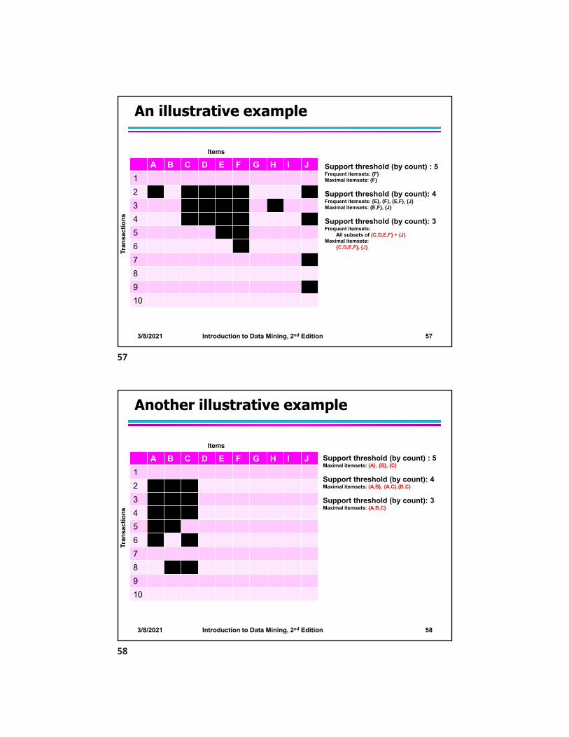
An illustrative example
Support threshold (by count) : 5Frequent itemsets: {F}Maximal itemsets: {F}
Support threshold (by count): 4Frequent itemsets: {E}, {F}, {E,F}, {J}Maximal itemsets: {E,F}, {J}
Support threshold (by count): 3Frequent itemsets:
All subsets of {C,D,E,F} + {J}Maximal itemsets:
{C,D,E,F}, {J}
A B C D E F G H I J
1
2
3
4
5
6
7
8
9
10
Items
Tran
sact
ion
s
3/8/2021 Introduction to Data Mining, 2nd Edition 58
Another illustrative example
Support threshold (by count) : 5Maximal itemsets: {A}, {B}, {C}
Support threshold (by count): 4Maximal itemsets: {A,B}, {A,C},{B,C}
Support threshold (by count): 3Maximal itemsets: {A,B,C}
A B C D E F G H I J
1
2
3
4
5
6
7
8
9
10
Tran
sact
ion
s
Items
57
58

3/8/2021 Introduction to Data Mining, 2nd Edition 59
Closed Itemset
An itemset X is closed if none of its immediate supersets has the same support as the itemset X.
X is not closed if at least one of its immediate supersets has support count as X.
3/8/2021 Introduction to Data Mining, 2nd Edition 60
Closed Itemset
An itemset X is closed if none of its immediate supersets has the same support as the itemset X.
X is not closed if at least one of its immediate supersets has support count as X.
TID Items1 {A,B}2 {B,C,D}3 {A,B,C,D}4 {A,B,D}5 {A,B,C,D}
Itemset Support{A} 4{B} 5{C} 3{D} 4
{A,B} 4{A,C} 2{A,D} 3{B,C} 3{B,D} 4{C,D} 3
Itemset Support{A,B,C} 2{A,B,D} 3{A,C,D} 2{B,C,D} 2
{A,B,C,D} 2
59
60
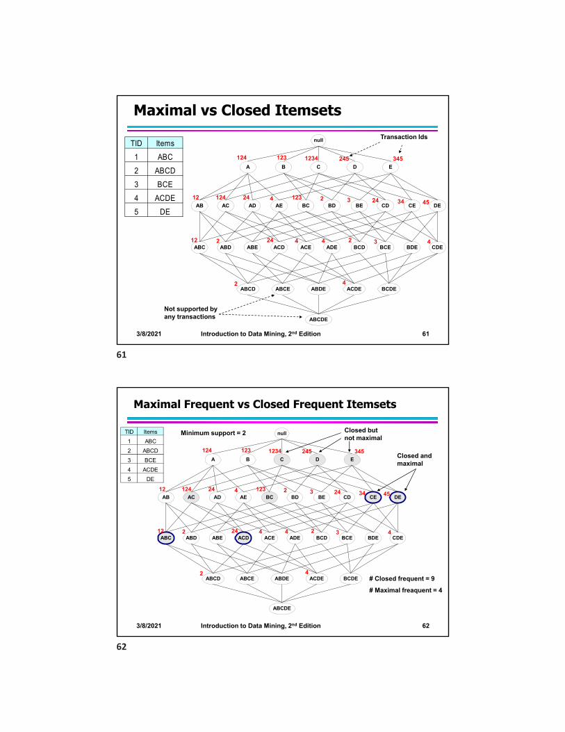
3/8/2021 Introduction to Data Mining, 2nd Edition 61
Maximal vs Closed Itemsets
TID Items
1 ABC
2 ABCD
3 BCE
4 ACDE
5 DE
null
AB AC AD AE BC BD BE CD CE DE
A B C D E
ABC ABD ABE ACD ACE ADE BCD BCE BDE CDE
ABCD ABCE ABDE ACDE BCDE
ABCDE
124 123 1234 245 345
12 124 24 4 123 2 3 24 34 45
12 2 24 4 4 2 3 4
2 4
Transaction Ids
Not supported by any transactions
3/8/2021 Introduction to Data Mining, 2nd Edition 62
null
AB AC AD AE BC BD BE CD CE DE
A B C D E
ABC ABD ABE ACD ACE ADE BCD BCE BDE CDE
ABCD ABCE ABDE ACDE BCDE
ABCDE
124 123 1234 245 345
12 124 24 4 123 2 3 24 34 45
12 2 24 4 4 2 3 4
2 4
Maximal Frequent vs Closed Frequent Itemsets
Minimum support = 2
# Closed frequent = 9
# Maximal freaquent = 4
Closed and maximal
Closed but not maximal
TID Items
1 ABC
2 ABCD
3 BCE
4 ACDE
5 DE
61
62

3/8/2021 Introduction to Data Mining, 2nd Edition 63
What are the Closed Itemsets in this Data?
TID A1 A2 A3 A4 A5 A6 A7 A8 A9 A10 B1 B2 B3 B4 B5 B6 B7 B8 B9 B10 C1 C2 C3 C4 C5 C6 C7 C8 C9 C101 1 1 1 1 1 1 1 1 1 1 0 0 0 0 0 0 0 0 0 0 0 0 0 0 0 0 0 0 0 02 1 1 1 1 1 1 1 1 1 1 0 0 0 0 0 0 0 0 0 0 0 0 0 0 0 0 0 0 0 03 1 1 1 1 1 1 1 1 1 1 0 0 0 0 0 0 0 0 0 0 0 0 0 0 0 0 0 0 0 04 1 1 1 1 1 1 1 1 1 1 0 0 0 0 0 0 0 0 0 0 0 0 0 0 0 0 0 0 0 05 1 1 1 1 1 1 1 1 1 1 0 0 0 0 0 0 0 0 0 0 0 0 0 0 0 0 0 0 0 06 0 0 0 0 0 0 0 0 0 0 1 1 1 1 1 1 1 1 1 1 0 0 0 0 0 0 0 0 0 07 0 0 0 0 0 0 0 0 0 0 1 1 1 1 1 1 1 1 1 1 0 0 0 0 0 0 0 0 0 08 0 0 0 0 0 0 0 0 0 0 1 1 1 1 1 1 1 1 1 1 0 0 0 0 0 0 0 0 0 09 0 0 0 0 0 0 0 0 0 0 1 1 1 1 1 1 1 1 1 1 0 0 0 0 0 0 0 0 0 010 0 0 0 0 0 0 0 0 0 0 1 1 1 1 1 1 1 1 1 1 0 0 0 0 0 0 0 0 0 011 0 0 0 0 0 0 0 0 0 0 0 0 0 0 0 0 0 0 0 0 1 1 1 1 1 1 1 1 1 112 0 0 0 0 0 0 0 0 0 0 0 0 0 0 0 0 0 0 0 0 1 1 1 1 1 1 1 1 1 113 0 0 0 0 0 0 0 0 0 0 0 0 0 0 0 0 0 0 0 0 1 1 1 1 1 1 1 1 1 114 0 0 0 0 0 0 0 0 0 0 0 0 0 0 0 0 0 0 0 0 1 1 1 1 1 1 1 1 1 115 0 0 0 0 0 0 0 0 0 0 0 0 0 0 0 0 0 0 0 0 1 1 1 1 1 1 1 1 1 1
(A1-A10)(B1-B10)(C1-C10)
3/8/2021 Introduction to Data Mining, 2nd Edition 64
Example 1
A B C D E F G H I J
1
2
3
4
5
6
7
8
9
10
Items
Tran
sact
ion
s
Itemsets Support(counts)
Closed itemsets
{C} 3
{D} 2
{C,D} 2
63
64

3/8/2021 Introduction to Data Mining, 2nd Edition 65
Example 1
A B C D E F G H I J
1
2
3
4
5
6
7
8
9
10
Items
Tran
sact
ion
s
Itemsets Support(counts)
Closed itemsets
{C} 3
{D} 2
{C,D} 2
3/8/2021 Introduction to Data Mining, 2nd Edition 66
Example 2
A B C D E F G H I J
1
2
3
4
5
6
7
8
9
10
Items
Tran
sact
ion
s
Itemsets Support(counts)
Closed itemsets
{C} 3
{D} 2
{E} 2
{C,D} 2
{C,E} 2
{D,E} 2
{C,D,E} 2
65
66

3/8/2021 Introduction to Data Mining, 2nd Edition 67
Example 2
A B C D E F G H I J
1
2
3
4
5
6
7
8
9
10
Items
Tran
sact
ion
s
Itemsets Support(counts)
Closed itemsets
{C} 3
{D} 2
{E} 2
{C,D} 2
{C,E} 2
{D,E} 2
{C,D,E} 2
3/8/2021 Introduction to Data Mining, 2nd Edition 68
Example 3
A B C D E F G H I J
1
2
3
4
5
6
7
8
9
10
Items
Tran
sact
ion
s
Closed itemsets: {C,D,E,F}, {C,F}
67
68

3/8/2021 Introduction to Data Mining, 2nd Edition 69
Example 4
A B C D E F G H I J
1
2
3
4
5
6
7
8
9
10
Items
Tran
sact
ion
s
Closed itemsets: {C,D,E,F}, {C}, {F}
3/8/2021 Introduction to Data Mining, 2nd Edition 70
Maximal vs Closed Itemsets
69
70

3/8/2021 Introduction to Data Mining, 2nd Edition 71
Example question
Given the following transaction data sets (dark cells indicate presence of an item in a transaction) and a support threshold of 20%, answer the following questions
a. What is the number of frequent itemsets for each dataset? Which dataset will produce the most number of frequent itemsets?
b. Which dataset will produce the longest frequent itemset?c. Which dataset will produce frequent itemsets with highest maximum support?d. Which dataset will produce frequent itemsets containing items with widely varying support
levels (i.e., itemsets containing items with mixed support, ranging from 20% to more than 70%)?
e. What is the number of maximal frequent itemsets for each dataset? Which dataset will produce the most number of maximal frequent itemsets?
f. What is the number of closed frequent itemsets for each dataset? Which dataset will produce the most number of closed frequent itemsets?
DataSet: A Data Set: B Data Set: C
3/8/2021 Introduction to Data Mining, 2nd Edition 72
Pattern Evaluation
Association rule algorithms can produce large number of rules
Interestingness measures can be used to prune/rank the patterns – In the original formulation, support & confidence are
the only measures used
71
72

3/8/2021 Introduction to Data Mining, 2nd Edition 73
Computing Interestingness Measure
Given X Y or {X,Y}, information needed to compute interestingness can be obtained from a contingency table
Y Y
X f11 f10 f1+
X f01 f00 fo+
f+1 f+0 N
Contingency table
f11: support of X and Yf10: support of X and Yf01: support of X and Yf00: support of X and Y
Used to define various measures
support, confidence, Gini,entropy, etc.
3/8/2021 Introduction to Data Mining, 2nd Edition 74
Drawback of Confidence
Association Rule: Tea Coffee
Confidence P(Coffee|Tea) = 150/200 = 0.75Confidence > 50%, meaning people who drink tea are more likely to drink coffee than not drink coffeeSo rule seems reasonable
Customers
Tea Coffee …
C1 0 1 …
C2 1 0 …
C3 1 1 …
C4 1 0 …
…
73
74

3/8/2021 Introduction to Data Mining, 2nd Edition 75
Drawback of Confidence
Coffee Coffee
Tea 150 50 200
Tea 650 150 800
800 200 1000
Association Rule: Tea Coffee
Confidence= P(Coffee|Tea) = 150/200 = 0.75
but P(Coffee) = 0.8, which means knowing that a person drinks tea reduces the probability that the person drinks coffee! Note that P(Coffee|Tea) = 650/800 = 0.8125
3/8/2021 Introduction to Data Mining, 2nd Edition 76
Drawback of Confidence
Association Rule: Tea HoneyConfidence P(Honey|Tea) = 100/200 = 0.50Confidence = 50%, which may mean that drinking tea has little influence whether honey is used or notSo rule seems uninterestingBut P(Honey) = 120/1000 = .12 (hence tea drinkers are far more likely to have honey
Customers
Tea Honey …
C1 0 1 …
C2 1 0 …
C3 1 1 …
C4 1 0 …
…
75
76

3/8/2021 Introduction to Data Mining, 2nd Edition 77
Measure for Association Rules
So, what kind of rules do we really want?– Confidence(X Y) should be sufficiently high
To ensure that people who buy X will more likely buy Y than not buy Y
– Confidence(X Y) > support(Y) Otherwise, rule will be misleading because having item X actually reduces the chance of having item Y in the same transaction
Is there any measure that capture this constraint?
– Answer: Yes. There are many of them.
3/8/2021 Introduction to Data Mining, 2nd Edition 78
Statistical Relationship between X and Y
The criterion confidence(X Y) = support(Y)
is equivalent to:– P(Y|X) = P(Y)
– P(X,Y) = P(X) P(Y) (X and Y are independent)
If P(X,Y) > P(X) P(Y) : X & Y are positively correlated
If P(X,Y) < P(X) P(Y) : X & Y are negatively correlated
77
78

3/8/2021 Introduction to Data Mining, 2nd Edition 79
Measures that take into account statistical dependence
)](1)[()](1)[(
)()(),(
)()(),(
)()(
),(
)(
)|(
YPYPXPXP
YPXPYXPtcoefficien
YPXPYXPPS
YPXP
YXPInterest
YP
XYPLift
lift is used for rules while interest is used for itemsets
3/8/2021 Introduction to Data Mining, 2nd Edition 80
Example: Lift/Interest
Coffee Coffee
Tea 150 50 200
Tea 650 150 800
800 200 1000
Association Rule: Tea Coffee
Confidence= P(Coffee|Tea) = 0.75but P(Coffee) = 0.8 Interest = 0.15 / (0.2×0.8) = 0.9375 (< 1, therefore is negatively associated)So, is it enough to use confidence/Interest for pruning?
79
80
3/8/2021 Introduction to Data Mining, 2nd Edition 81
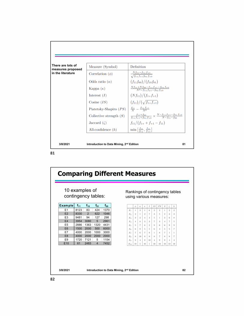
There are lots of measures proposed in the literature
3/8/2021 Introduction to Data Mining, 2nd Edition 82
Comparing Different Measures
Example f11 f10 f01 f00
E1 8123 83 424 1370E2 8330 2 622 1046E3 9481 94 127 298E4 3954 3080 5 2961E5 2886 1363 1320 4431E6 1500 2000 500 6000E7 4000 2000 1000 3000E8 4000 2000 2000 2000E9 1720 7121 5 1154
E10 61 2483 4 7452
10 examples of contingency tables:
Rankings of contingency tables using various measures:
81
82

3/8/2021 Introduction to Data Mining, 2nd Edition 83
Property under Inversion Operation
Transaction 1
Transaction N
.
.
.
.
.
3/8/2021 Introduction to Data Mining, 2nd Edition 84
Property under Inversion Operation
Transaction 1
Transaction N
.
.
.
.
.
Correlation: -0.1667 -0.1667IS/cosine 0.0 0.825
83
84

3/8/2021 Introduction to Data Mining, 2nd Edition 85
Invariant measures:
cosine, Jaccard, All-confidence, confidence
Non-invariant measures:
correlation, Interest/Lift, odds ratio, etc
Property under Null Addition
3/8/2021 Introduction to Data Mining, 2nd Edition 86
Property under Row/Column Scaling
Male Female
High 30 20 50
Low 40 10 50
70 30 100
Male Female
High 60 60 120
Low 80 30 110
140 90 230
Grade-Gender Example (Mosteller, 1968):
Mosteller: Underlying association should be independent ofthe relative number of male and female studentsin the samples
Odds-Ratio ((f11+f00 )/(f10+f10)) has this property
2x 3x
85
86

3/8/2021 Introduction to Data Mining, 2nd Edition 87
Property under Row/Column Scaling
Covid-Positive
Covid-Free
Mask 20 30 50
No-Mask
40 10 50
60 40 100
Relationship between Mask use and susceptibility to Covid:
Mosteller: Underlying association should be independent ofthe relative number of Covid-positive and Covid-free subjects
Odds-Ratio ((f11+f00 )/(f10+f10)) has this property
2x 10x
Covid-Positive
Covid-Free
Mask 40 300 340
No-Mask
80 100 180
120 400 520
3/8/2021 Introduction to Data Mining, 2nd Edition 88
Different Measures have Different Properties
87
88

3/8/2021 Introduction to Data Mining, 2nd Edition 89
Simpson’s Paradox
Observed relationship in data may be influenced by the presence of other confounding factors (hidden variables)– Hidden variables may cause the observed relationship
to disappear or reverse its direction!
Proper stratification is needed to avoid generating spurious patterns
3/8/2021 Introduction to Data Mining, 2nd Edition 90
Simpson’s Paradox
Recovery rate from Covid– Hospital A: 80%
– Hospital B: 90%
Which hospital is better?
89
90

3/8/2021 Introduction to Data Mining, 2nd Edition 91
Simpson’s Paradox
Recovery rate from Covid– Hospital A: 80%
– Hospital B: 90%
Which hospital is better?
Covid recovery rate on older population– Hospital A: 50%
– Hospital B: 30%
Covid recovery rate on younger population– Hospital A: 99%
– Hospital B: 98%
3/8/2021 Introduction to Data Mining, 2nd Edition 92
Simpson’s Paradox
Covid-19 death: (per 100,000 of population)– County A: 15
– County B: 10
Which state is managing the pandemic better?
91
92

3/8/2021 Introduction to Data Mining, 2nd Edition 93
Simpson’s Paradox
Covid-19 death: (per 100,000 of population)– County A: 15
– County B: 10
Which state is managing the pandemic better?
Covid death rate on older population– County A: 20
– County B: 40
Covid death rate on younger population– County A: 2
– County B: 5
3/8/2021 Introduction to Data Mining, 2nd Edition 94
Effect of Support Distribution on Association Mining
Many real data sets have skewed support distribution
Support distribution of a retail data set
Rank of item (in log scale)
Few items with high support
Many items with low support
93
94

3/8/2021 Introduction to Data Mining, 2nd Edition 95
Effect of Support Distribution
Difficult to set the appropriate minsup threshold– If minsup is too high, we could miss itemsets involving
interesting rare items (e.g., {caviar, vodka})
– If minsup is too low, it is computationally expensive and the number of itemsets is very large
3/8/2021 Introduction to Data Mining, 2nd Edition 96
Cross-Support Patterns
0
20
40
60
80
100
0 500 1000 1500 2000
Sup
port
(%
)
Sorted Items
The Support Distribution of Pumsb Dataset
milkcaviar
A cross-support pattern involves items with varying degree of support• Example: {caviar,milk}
How to avoid such patterns?
95
96
3/8/2021 Introduction to Data Mining, 2nd Edition 97
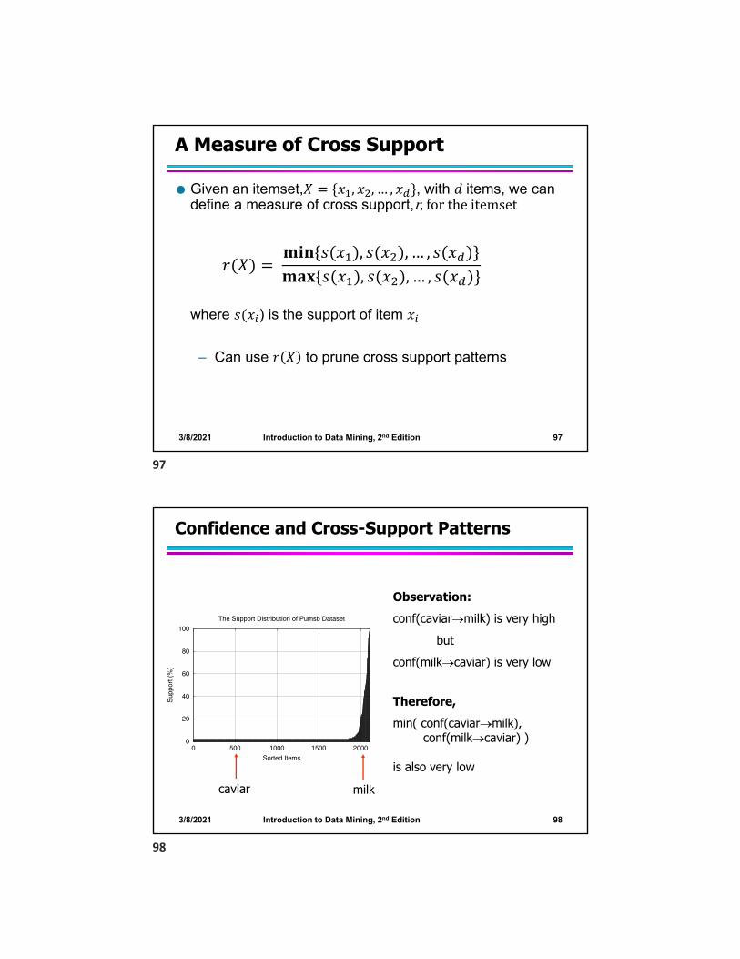
A Measure of Cross Support
Given an itemset,𝑋 𝑥 , 𝑥 , … , 𝑥 , with 𝑑 items, we can define a measure of cross support,r, for the itemset
where 𝑠 𝑥 ) is the support of item 𝑥
– Can use 𝑟 𝑋 to prune cross support patterns
𝑟 𝑋 𝐦𝐢𝐧 𝑠 𝑥 , 𝑠 𝑥 , … , 𝑠 𝑥𝐦𝐚𝐱 𝑠 𝑥 , 𝑠 𝑥 , … , 𝑠 𝑥
3/8/2021 Introduction to Data Mining, 2nd Edition 98
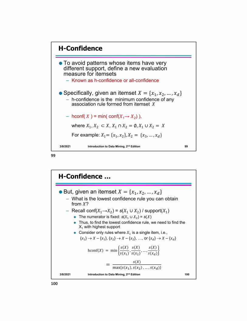
Confidence and Cross-Support Patterns
0
20
40
60
80
100
0 500 1000 1500 2000
Sup
port
(%
)
Sorted Items
The Support Distribution of Pumsb Dataset
milkcaviar
Observation:conf(caviarmilk) is very high
butconf(milkcaviar) is very low
Therefore,min( conf(caviarmilk),
conf(milkcaviar) )
is also very low
97
98
3/8/2021 Introduction to Data Mining, 2nd Edition 99
H-Confidence
To avoid patterns whose items have very different support, define a new evaluation measure for itemsets– Known as h-confidence or all-confidence
Specifically, given an itemset 𝑋 𝑥 , 𝑥 , … , 𝑥– h-confidence is the minimum confidence of any
association rule formed from itemset 𝑋
– hconf( 𝑋 ) = min( conf(𝑋1→ 𝑋2) ),
where 𝑋 ,𝑋 ⊂ 𝑋, 𝑋 ∩𝑋 ∅,𝑋 ∪ 𝑋 𝑋
For example: 𝑋 𝑥 , 𝑥 ,𝑋 𝑥 , … , 𝑥
3/8/2021 Introduction to Data Mining, 2nd Edition 100
H-Confidence …
But, given an itemset 𝑋 𝑥 , 𝑥 , … , 𝑥– What is the lowest confidence rule you can obtain
from 𝑋?– Recall conf(𝑋 →𝑋 ) = s(𝑋 ∪ 𝑋 ) / support(𝑋 )
The numerator is fixed: s(𝑋 ∪ 𝑋 ) = s(X ) Thus, to find the lowest confidence rule, we need to find the
X1 with highest support
Consider only rules where 𝑋 is a single item, i.e.,
{𝑥 } 𝑋 – {𝑥 }, {𝑥 } 𝑋 – {𝑥 }, …, or {𝑥 } 𝑋 – {𝑥 }
hconf 𝑋 min𝑠 𝑋𝑠 𝑥
,𝑠 𝑋𝑠 𝑥
, … ,𝑠 𝑋𝑠 𝑥
, , … ,
99
100

3/8/2021 Introduction to Data Mining, 2nd Edition 101
Cross Support and H-confidence
By the anti-montone property of support
𝑠 𝑋 min 𝑠 𝑥 , 𝑠 𝑥 , … , 𝑠 𝑥 Therefore, we can derive a relationship between
the h-confidence and cross support of an itemsethconf 𝑋
𝑠 𝑋max 𝑠 𝑥 , 𝑠 𝑥 , … , 𝑠 𝑥
, , …,
, , … ,
𝑟 𝑋
Thus, hconf 𝑋 𝑟 𝑋
3/8/2021 Introduction to Data Mining, 2nd Edition 102
Cross Support and H-confidence …
Since, hconf 𝑋 𝑟 𝑋 , we can eliminate cross support patterns by finding patterns with h-confidence < hc, a user set threshold
Notice that
0 hconf 𝑋 𝑟 𝑋 1
Any itemset satisfying a given h-confidence threshold, hc, is called a hyperclique
H-confidence can be used instead of or in conjunction with support
101
102

3/8/2021 Introduction to Data Mining, 2nd Edition 103
Properties of Hypercliques
Hypercliques are itemsets, but not necessarily frequent itemsets– Good for finding low support patterns
H-confidence is anti-monotone
Can define closed and maximal hypercliques in terms of h-confidence– A hyperclique X is closed if none of its immediate
supersets has the same h-confidence as X– A hyperclique X is maximal if hconf 𝑋 h and none
of its immediate supersets, Y, have hconf 𝑌 h
3/8/2021 Introduction to Data Mining, 2nd Edition 104
Properties of Hypercliques …
Hypercliques have the high-affinity property– Think of the individual items as sparse binary vectors– h-confidence gives us information about their pairwise
Jaccard and cosine similarity Assume 𝑥 and 𝑥 are any two items in an itemset X Jaccard 𝑥 , 𝑥 hconf X /2 cos 𝑥 , 𝑥 hconf X
– Hypercliques that have a high h-confidence consist of very similar items as measured by Jaccard and cosine
The items in a hyperclique cannot have widely different support– Allows for more efficient pruning
103
104

3/8/2021 Introduction to Data Mining, 2nd Edition 105
Example Applications of Hypercliques
Hypercliques are used to find strongly coherent groups of items– Words that occur together
in documents– Proteins in a protein
interaction network
In the figure at the right, a gene ontology hierarchy for biological process shows that the identified proteins in the hyperclique (PRE2, …, SCL1) perform the same function and are involved in the same biological process
105