chap 3 fea for nonlinear elastic problems - uf mae · 1 chap 3 fea for nonlinear elastic problems...

1

CHAP 3

FEA for Nonlinear Elastic Problems

Nam-Ho Kim

2

Introduction• Linear systems

– Infinitesimal deformation: no significant difference between the deformed and undeformed shapes

– Stress and strain are defined in the undeformed shape– The weak form is integrated over the undeformed shape

• Large deformation problem– The difference between the deformed and undeformed shapes is

large enough that they cannot be treated the same– The definitions of stress and strain should be modified from the

assumption of small deformation– The relation between stress and strain becomes nonlinear as

deformation increases• This chapter will focus on how to calculate the residual

and tangent stiffness for a nonlinear elasticity model

3

Introduction• Frame of Reference

– The weak form must be expressed based on a frame of reference– Often initial (undeformed) geometry or current (deformed)

geometry are used for the frame of reference– proper definitions of stress and strain must be used according to

the frame of reference• Total Lagrangian Formulation: initial (undeformed)

geometry as a reference• Updated Lagrangian Formulation: current (deformed)

geometry• Two formulations are theoretically identical to express

the structural equilibrium, but numerically different because different stress and strain definitions are used

4

Table of Contents• 3.2. Stress and Strain Measures in Large Deformation• 3.3. Nonlinear Elastic Analysis• 3.4. Critical Load Analysis• 3.5. Hyperelastic Materials• 3.6. Finite Element Formulation for Nonlinear Elasticity• 3.7. MATLAB Code for Hyperelastic Material Model• 3.8. Nonlinear Elastic Analysis Using Commercial Finite

Element Programs• 3.9. Fitting Hyperelastic Material Parameters from Test

Data• 3.9. Summary• 3.10.Exercises

5

Stress and Strain Measures3.2

6

Goals – Stress & Strain Measures

• Definition of a nonlinear elastic problem

• Understand the deformation gradient?

• What are Lagrangian and Eulerian strains?

• What is polar decomposition and how to do it?

• How to express the deformation of an area and volume

• What are Piola-Kirchhoff and Cauchy stresses?

7

Mild vs. Rough Nonlinearity

• Mild Nonlinear Problems (Chap 3)

– Continuous, history-independent nonlinear relations between

stress and strain

– Nonlinear elasticity, Geometric nonlinearity, and deformation-

dependent loads

• Rough Nonlinear Problems (Chap 4 & 5)

– Equality and/or inequality constraints in constitutive relations

– History-dependent nonlinear relations between stress and strain

– Elastoplasticity and contact problems

8

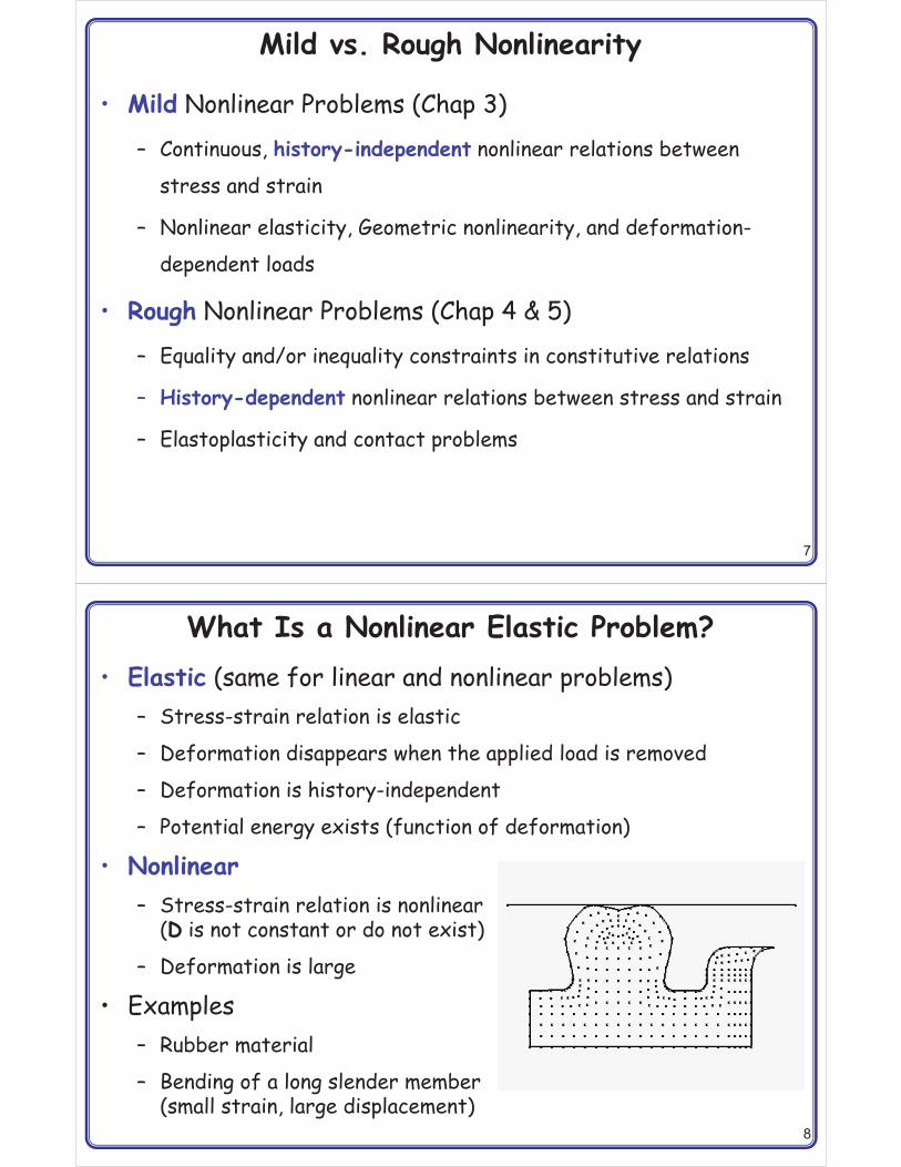
What Is a Nonlinear Elastic Problem?• Elastic (same for linear and nonlinear problems)

– Stress-strain relation is elastic

– Deformation disappears when the applied load is removed

– Deformation is history-independent

– Potential energy exists (function of deformation)

• Nonlinear– Stress-strain relation is nonlinear

(D is not constant or do not exist)

– Deformation is large

• Examples– Rubber material

– Bending of a long slender member(small strain, large displacement)

9

Reference Frame of Stress and Strain• Force and displacement (vector) are independent of the

configuration frame in which they are defined (Reference Frame Indifference)

• Stress and strain (tensor) depend on the configuration

• Total Lagrangian or Material Stress/Strain: when the reference frame is undeformed configuration

• Updated Lagrangian or Spatial Stress/Strain: when the reference frame is deformed configuration

• Question: What is the reference frame in linear problems?

10

Deformation and Mapping• Initial domain �0 is deformed to �x

– We can think of this as a mapping from �0 to �x

• X: material point in �0 x: material point in �x

• Material point P in �0 is deformed to Q in �x

� �x X u

displacement

� � � �( , t) ( , t)x X X u X

�0

�x

X x

u

PQ

�

1, :�� One-to-one mappingContinuously differentiable

11

Deformation Gradient• Infinitesimal length dX in �0 deforms to dx in �x

• Remember that the mapping is continuously differentiable

• Deformation gradient:

– gradient of mapping �

– Second-order tensor, Depend on both �0 and �x

– Due to one-to-one mapping:

– F includes both deformation and rigid-body rotation

�0

�x

u dxdXP

QP'

Q'd d d d�

� � ��xx X x F XX

iij

j

xFX�

�� 0

��

�uF 1 1 uX

det J 0. �F

ij

0 x

[ ],

,

� �

� � � �

� �

1

X x

1d d��X F x

12

Example – Uniform Extension• Uniform extension of a cube in all three directions

• Continuity requirement: Why?• Deformation gradient:

• : uniform expansion (dilatation) or contraction• Volume change

– Initial volume:

– Deformed volume:

1 1 1 2 2 2 3 3 3x X , x X , x X� � �

1

2

3

0 00 00 0

� ��

F

i 0 �

1 2 3 � �

0 1 2 3dV dX dX dX�

x 1 2 3 1 2 3 1 2 3 1 2 3 0dV dx dx dx dX dX dX dV� � �

13

Green-Lagrange Strain• Why different strains?• Length change:

• Right Cauchy-Green Deformation Tensor

• Green-Lagrange Strain Tensor

2 2 T T

T T T

T T

d d d d d dd d d dd ( )d

� � �

� �

� �

x X x x X XX F F X X XX F F 1 X

Ratio of length change

T�C F F

1 ( )2

� �E C 1

dXdx

The effect of rotation is eliminated

To match with infinitesimal strain

14

Green-Lagrange Strain cont.• Properties:

– E is symmetric: ET = E

– No deformation: F = 1, E = 0

– When ,

– E = 0 for a rigid-body motion, but

� �

T T

T T10 0 0 02

12� ��

� � ��

u u u uEX X X Xu u u u

jiij

j i

uu12 X X

��

Displacement gradient

Higher-order term

0 1 ��u � �T0 0

1 �2

� � �E u u

�� 0

15

Example – Rigid-Body Rotation• Rigid-body rotation

• Approach 1: using deformation gradient

� � � � �

1 1 2

2 1 2

3 3

x X cos X sinx X sin X cosx X

� � ��

cos sin 0sin cos 0

0 0 1F

� ��

T1 0 00 1 00 0 1

F F

� � �T12 ( )E F F 1 0

Green-Lagrange strain removes rigid-body rotation from deformation

16

Example – Rigid-Body Rotation cont.• Approach 2: using displacement gradient

� � � � � � � � � ��

1 1 1 1 2

2 2 2 1 2

3 3 3

u x X X (cos 1) X sinu x X X sin X (cos 1)u x X 0

� � � ��

0

cos 1 sin 0sin cos 1 0

0 0 0u

� � ��

T0 0

2(1 cos ) 0 00 2(1 cos ) 00 0 0

u u

� � � �T T10 0 0 02 ( )E u u u u 0

17

Example – Rigid-Body Rotation cont.• What happens to engineering strain?

� � � � � � � � � ��

1 1 1 1 2

2 2 2 1 2

3 3 3

u x X X (cos 1) X sinu x X X sin X (cos 1)u x X 0

��

�cos 1 0 0

0 cos 1 00 0 0

Engineering strain is unable to take care of rigid-body rotation

18

Eulerian (Almansi) Strain Tensor

• Length change:

• Left Cauchy-Green Deformation Tensor

• Eulerian (Almansi) Strain Tensor

� �

� �

�

� � �

� �

� �

� �

2 2 T T

T T T 1

T T 1

T 1

d d d d d dd d d dd ( )dd ( )d

x X x x X Xx x x F F xx 1 F F xx 1 b x

� Tb FF

�� 11 ( )2

e 1 b

Reference is deformed (current) configuration

b–1: Finger tensor

19

Eulerian Strain Tensor cont.

• Properties

– Symmetric

– Approach engineering strain when

– In terms of displacement gradient

• Relation between E and e

� �

� ��

� � �

T T

T Tx x x x

1212

u u u uex x x x

u u u u

� �

�x xSpatial gradient

� TE F eF

��

�1u

x

20

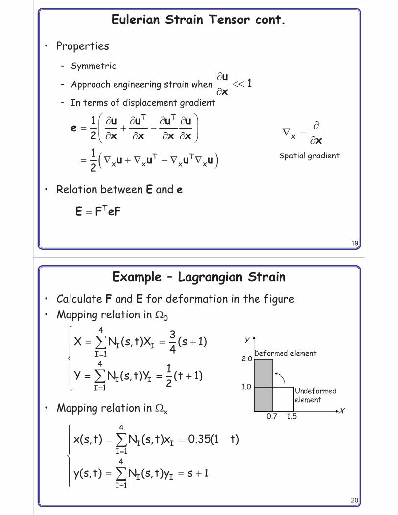
Example – Lagrangian Strain• Calculate F and E for deformation in the figure• Mapping relation in �0

• Mapping relation in �x 1.5

1.0

X

Y

Undeformed element

Deformed element2.0

0.7

�

�

!� � �"

"#" � � �"$

%

%

4

I II 14

I II 1

3X N (s, t)X (s 1)41Y N (s, t)Y (t 1)2

�

�

!� � �"

"#" � � �"$

%

%

4

I II 14

I II 1

x(s, t) N (s, t)x 0.35(1 t)

y(s, t) N (s, t)y s 1

21

Example – Lagrangian Strain cont.• Deformation gradient

• Green-Lagrange Strain

�0

�x

u dxdXP

QP'

Q'

( , )s tX( , )s tx

Referencedomain (s, t)

� � ��

��

��

0 .35 4 / 3 01 0 0 2

0 0.74 / 3 0

x x sFX s X

� ��

T 0.389 01 ( )2 0 0.255

E F F 1 Tension in X1 dir.Compression in X2 dir.

22

Example – Lagrangian Strain cont.• Almansi Strain

• Engineering Strain

� �� & � � �

� �T 0.49 0

0 1.78b F F

� ��

� �11

20.52 00 0.22

e 1 b

� ��

01 0.7

1.33 1u F 1

� � ��

� T10 02

1 0.320.32 1

u u

Which strain is consistent with actual deformation?

Compression in x1 dir.Tension in x2 dir.

Artificial shear deform.Inconsistent normal deform.

23

Example – Uniaxial Tension• Uniaxial tension of incompressible material ( 1 = '�'()• From incompressibility

• Deformation gradient and deformation tensor

• G-L Strain

� � � � � 1/21 2 3 2 31

�

�

� ��

� � ��

1/2

1/2

0 00 00 0

F �

�

� � � �

� � ��

2

1

1

0 00 00 0

C

�

�

� � ��

� ��

2

1

1

1 0 01 0 1 02

0 0 1E

� � �

1 1 1

2 2 2

3 3 3

x Xx Xx X

24

Example – Uniaxial Tension• Almansi Strain (b = C)

• Engineering Strain

• Difference

��

� � � ��

21 0 01 0 1 02

0 0 1e

�

�

� � � �

� � ��

2

10 0

0 00 0

b

�

�

��

� ��

� 1/2

1/2

1 0 00 1 00 0 1

�� 2 211 11 11

1 1E ( 1) e (1 ) 12 2

10%strain

25

Polar Decomposition

• Want to separate deformation from rigid-body rotation

• Similar to principal directions of strain

• Unique decomposition of deformation gradient

– Q: orthogonal tensor (rigid-body rotation)

– U, V: right- and left-stretch tensor (symmetric)

• U and V have the same eigenvalues (principal stretches),

but different eigenvectors

� �F QU VQ

26

Polar Decomposition cont.

• Eigenvectors of U: E1, E2, E3

• Eigenvectors of V: e1, e2, e3

• Eigenvalues of U and V: 1, 2, 3

Q

Q

V

U

E1 E2

E3

�1E1�2E2

�3E3

e1e2

e3

�1e1

�2e2

�3e3

�F QU

�F VQ� & &� & &

d dd

x Q U XV Q X

27

Polar Decomposition cont.• Relation between U and C

– U and C have the same eigenvectors.

– Eigenvalue of U is the square root of that of C

• How to calculate U from C?• Let eigenvectors of C be• Then, where

� �2U C U C

1 2 3[ ]� E E E�T� C) � �

� � � �

) � � ��

21

22

23

0 00 00 0

Deformation tensor in principal directions

28

Polar Decomposition cont.

• And

• General Deformation

1. Stretch in principal directions

2. Rigid-body rotation

3. Rigid-body translation

� � � �d d dx F X b QU X b

� �� ) �TU

� �� ) � � ��

1

2

3

0 00 00 0

�� *%

3

i i ii 1

U E E

�� *%

3

i i ii 1

V e e

�� *%

3

i ii 1

Q e E

�� *%

3

i i ii 1

F e E

�� *%

32i i i

i 1C E E

�� *%

32i i i

i 1b e e

Useful formulas

29

Generalized Lagrangian Strain• G-L strain is a special case of general form of Lagrangian

strain tensors (Hill, 1968)

� �� 2mm

12m

E U 1

30

Example – Polar Decomposition• Simple shear problem

• Deformation gradient

• Deformation tensor

• Find eigenvalues and eigenvectors of C

� �!" �#" �$

1 1 2

2 2

3 3

x X kXx Xx X

�2k3

X1, x1

X2, x2

� ��

1 k0 1

F

� ��

� � ��

23T

2 7233

11 kk k 1

C F F

� � � � � �

� � �1 2

3 31 11 22 2 2 2

3, 1 3,E E

X1

X2

E2

E1

60o

31

Example – Polar Decomposition cont.

• In E1 – E2 coordinates

• Principal Direction Matrix

• Deformation tensor in principal directions

• Stretch tensor

� �+ � � � �

� �)

3 00 1 3

C

1 21 2 3 2[ ]3 2 1 2

� ��

� �� E E

� & &) � �T C

3 00 1 3

� ��

)

� �� & & � � �

� �� ) �T 3 2 1 2

1 2 5 2 3U

32

Example – Polar Decomposition cont.• How U deforms a square?

• Rotational Tensor

– 30o clockwise rotation

1 3 2 1 21 2 3 2

� � �� & � � �

�� Q F U

1 21 03 2 ,0 11 2 5 2 3

! , ! ,! , ! ,& � & �# - # - # - # -$ . $ .$ . $ .

U U

X1, x1

X2, x2

30o

X1, x1

X2, x2

30o

1 21 1.153 2 ,0 11 2 5 2 3

! , ! ,! , ! ,& � & �# - # - # - # -

$ . $ .$ . $ .Q Q

5 3 6 1 21 2 3 2

T � �� & � � �

� �� V F Q

33

Example – Polar Decomposition cont.• A straight line will deform to

• Consider a diagonal line: / = 45o

• Consider a circle

� /2 1X X tan

� �/

� � �� /

� � �

1 1 2 2 2

2 1 21

1 2tan

X x kx , X xx (x kx )tanx k x

� � � 0�

2

1

x 1tan 24.9x 1 k

� �

� � �

� � � �

2 2 21 2

2 2 21 2 2

2 2 2 21 1 2 2

X X r(x kx ) x rx 2kx x (1 k )x r Equation of ellipse

X1, x1

X2, x2

25o

X1, x1

X2, x2

34

Deformation of a Volume• Infinitesimal volume by three vectors

– Undeformed:

– Deformed:� & 1 �1 2 3 1 2 3

0 rst r s tdV d (d d ) e dX dX dXX X X

� & 1 �1 2 3 1 2 3x ijk i j kdV d (d d ) e dx dx dxx x x

�

��

� ��

� � �

��

1 2 3x ijk i j k

j1 2 3kiijk r s t

r s t

j 1 2 3kiijk r s t

r s t1 2 3

rst r s t

0

dV e dx dx dxx xxe dX dX dX

X X Xx xxe dX dX dX

X X Xe J dX dX dX

JdV

From Continuum Mechanics

�ijk ir js kt rste a a a e deta� � 1 2 3J detF

dX1

dX3

dX2

dx1dx3

dx2

35

Deformation of a Volume cont.• Volume change

• Volumetric Strain

• Incompressible condition: J = 1• Transformation of integral domain

�� x 0

0

dV dV J 1dV

�x 0dV JdV

x 0fd fJd

� �� 222 222

36

Example - Uniaxial Deformation of a Beam• Initial dimension of L0×h0×h0 deforms to L×h×h


• Constant volume

� ��

1 1 1 1 0

2 2 2 2 0

3 3 3 3 0

x X L / Lx X h / hx X h / h

� ��

1

2

3

0 00 00 0

F� �

� ��

� �

1 2 32

0 0 0 0

J det

L h LAL h L A

F

� � � �0 00 0

L LJ 1 h h A AL L

L0

h0

h0

Lh

h

37

Deformation of an Area• Relationship between dS0 and dSx

dSxdx1

n

SxxdS0

dX1

N

S0

X

F(X)

dX2 dx2

Undeformed Deformed

� 1 �

� 1 �

1 2 1 20 i 0 ijk j k

1 2 1 2x r x rst s t

dS d d NdS e dX dX

dS d d n dS e dx dx

N X X

n x x

� ��

� �j 1 2k

i 0 ijk s ts t

X XNdS e dx dxx x

� ��

� � � �j 1 2ki i

i 0 ijk s tr r s t

X XX XNdS e dx dxx x x x

�1�

i

r

Xx

38

Deformation of an Area cont..• Results from Continuum Mechanics

• Use the second relation:

��

� � � �1j 1 2 1 2ki i

i 0 ijk s t rst s tr r s t

X XX XNdS e dx dx e dx dxx x x x

F

�

� � ��

� � �

� ��

� � �

r s tijk rst

i j k

j1 kirst ijk

r s t

x x xe eX X X

X XXe e .x x x

F

F

r xn dS

�� &Tx 0dS J dSn F N

TT

T

��

�

&& � �

&F Nn F N nF N

�

�� Tx 0dS J ( ) ( ) dSF x N X

39

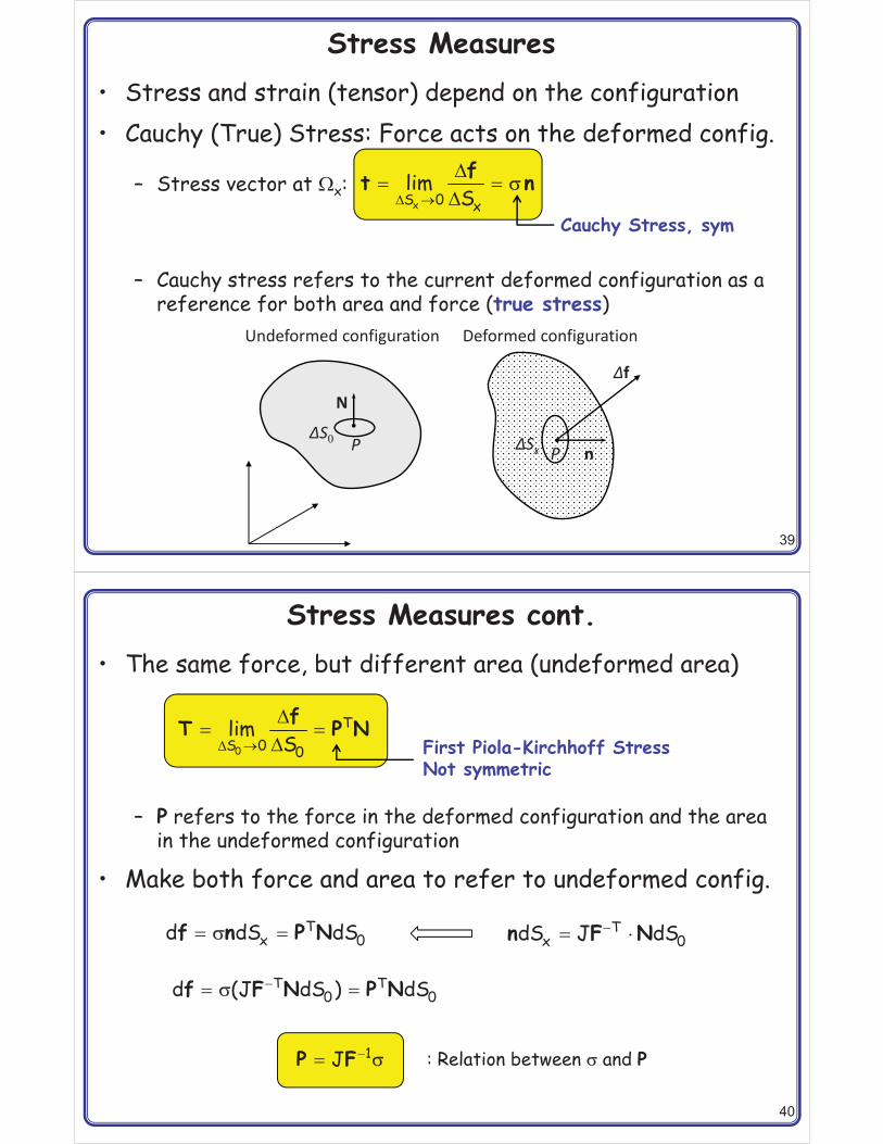
Stress Measures• Stress and strain (tensor) depend on the configuration • Cauchy (True) Stress: Force acts on the deformed config.

– Stress vector at �x:

– Cauchy stress refers to the current deformed configuration as a reference for both area and force (true stress)

P

N

�S0P n�Sx

�f

Undeformed configuration Deformed�configuration

3 4

3� �

3xS 0 xlim

Sft n5

Cauchy Stress, sym

40

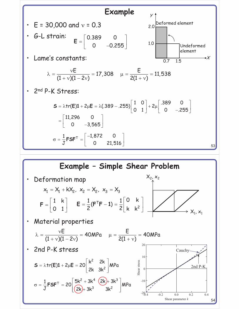
Stress Measures cont.• The same force, but different area (undeformed area)

– P refers to the force in the deformed configuration and the area in the undeformed configuration

• Make both force and area to refer to undeformed config.

3 4

3� �

30

TS 0 0lim

SfT P N

First Piola-Kirchhoff StressNot symmetric

� � Tx 0d dS dSf n P N5 �� &T

x 0dS J dSn F N

�� 1JP F 5

�� T T0 0d (J dS ) dSf F N P N5

: Relation between 5 and P

41

Stress Measures cont.• Unsymmetric property of P makes it difficult to use

– Remember we used the symmetric property of stress & strain several times in linear problems

• Make P symmetric by multiplying with F-T

– Just convenient mathematical quantities

• Further simplification is possible by handling J differently

� � �� & � & &T 1 TJS P F F F5

Second Piola-Kirchhoff Stress, symmetric

� & & T1JF S F5

� � & & TJ F S F6 5

Kirchhoff Stress, symmetric

42

Stress Measures cont.• Example

• Observation– For linear problems (small deformation):

– For linear problems (small deformation):

– S and E are conjugate in energy

– S and E are invariant in rigid-body motion

� � �� 222 222 222

x 0 0x 0 0: d : Jd : d5 � 5 � 6 �

Integration can be done in �0

� � �P S5 6

� �E e�

43

Example – Uniaxial Tension• Cauchy (true) stress: , 522 = 533 = 512 = 523 = 513 = 0• Deformation gradient:

• First P-K stress

• Second P-K stress

L0

h0

h0

Lh

hF

5 �11FA

�

� �

�

� � � �

� ��

11

1 12

13

0 00 0 , J 10 0

F

� �� & & � � � �

21 T

11 11 2 2 20 11 0 0

F 1 F A FA FS (J )A A AA A

F F5

��

111 11

1 0 0

F 1 F A FP (JA A A A

F 5� �

No clear physical meaning

44

Summary• Nonlinear elastic problems use different measures of

stress and strain due to changes in the reference frame• Lagrangian strain is independent of rigid-body rotation,

but engineering strain is not• Any deformation can be uniquely decomposed into rigid-

body rotation and stretch• The determinant of deformation gradient is related to the

volume change, while the deformation gradient and surface normal are related to the area change

• Four different stress measures are defined based on the reference frame.

• All stress and strain measures are identical when the deformation is infinitesimal

45

Nonlinear Elastic Analysis3.3

46

Goals• Understanding the principle of minimum potential energy

– Understand the concept of variation

• Understanding St. Venant-Kirchhoff material• How to obtain the governing equation for nonlinear elastic

problem• What is the total Lagrangian formulation?• What is the updated Lagrangian formulation?• Understanding the linearization process

47

Numerical Methods for Nonlinear Elastic Problem• We will obtain the variational equation using the principle

of minimum potential energy– Only possible for elastic materials (potential exists)

• The N-R method will be used (need Jacobian matrix)• Total Lagrangian (material) formulation uses the

undeformed configuration as a reference, while the updated Lagrangian (spatial) uses the current configuration as a reference

• The total and updated Lagrangian formulations are mathematically equivalent but have different aspects in computation

48

Total Lagrangian Formulation• Using incremental force method and N-R method

– Total No. of load steps (N), current load step (n)

• Assume that the solution has converged up to tn

• Want to find the equilibrium state at tn+1

� � � 3n 1 n nf f f

0�

n�

X x

nu�u

Undeformed configuration(known)

Last�converged�configuration(known)

Current�configuration(unknown)

0PnP

n+1P

n+1�

Iteration

49

Total Lagrangian Formulation cont.• In TL, the undeformed configuration is the reference• 2nd P-K stress (S) and G-L strain (E) are the natural choice• In elastic material, strain energy density W exists, such

that

• We need to express W in terms of E

Wstressstrain�

��

50

Strain Energy Density and Stress Measures• By differentiating strain energy density with respect to

proper strains, we can obtain stresses• When W(E) is given

• When W(F) is given

• It is difficult to have W(�) because � depends on rigid-body rotation. Instead, we will use invariants in Section 3.5

W( )��

�ES

E

TW W W:� � � �� & � & �

� � � �E F F S P

F E F E

Second P-K stress

First P-K stress

51

St. Venant-Kirchhoff Material• Strain energy density for St. Venant-Kirchhoff material

• Fourth-order constitutive tensor (isotropic material)

– Lame’s constants:

– Identity tensor (2nd order):

– Identity tensor (4th order):

– Tensor product:

12W( ) : :�E E D E Contraction operator: � ij ij: a ba b

2� * � 7D 1 1 I8

� 7 �� 8 � 8 � 8

E E(1 )(1 2 ) 2(1 )

� �ij[ ]1� � � � � �1

ijkl ik jl il jk2I ( )

� 9� � � � �ii 11 22 33

: , 2nd-order sym.: tr( ) a a a a

I a a a1 a a

* � ij kla a (4th-order)a a

52

St. Venant-Kirchhoff Material cont.• Stress calculation

– differentiate strain energy density

– Limited to small strain but large rotation

– Rigid-body rotation is removed and only the stretch tensor contributes to the strain

– Can show

W( ) : tr( ) 2�� 7

�ES D E E 1 E

E

T T T 21 1 12 2 2( ) ( ) ( )� � � � � �E F F 1 U Q Qu 1 U 1

W W2� ��

SE C

Deformation tensor

53

Example• E = 30,000 and 8 = 0.3• G-L strain:

• Lame’s constants:

• 2nd P-K Stress:

1.5

1.0

X

Y

Undeformed element

Deformed element2.0

0.7

� ��

0.389 00 0.255

E

8 � � 7 � �

� 8 � 8 � 8E E17,308 11,538

(1 )(1 2 ) 2(1 )

� � � �� 7 � � � 7� � � ��

� � ��

1 0 .389 0tr( ) 2 (.389 .255) 20 1 0 .255

11,296 00 3,565

S E 1 E

��

� �T 1,872 01

J 0 21,516FSF5

54

Example – Simple Shear Problem• Deformation map

• Material properties

• 2nd P-K stress

� � � �1 1 2 2 2 3 3x X kX , x X , x X

X1, x1

X2, x2

� ��

� �T

20 k1 1( )

2 2 k kE F F 1� �

� � ��

1 k0 1

F

8 � � 7 � �

� 8 � 8 � 8E E40MPa 40MPa

(1 )(1 2 ) 2(1 )

� �� 7 � � �

� ��

2

2k 2ktr( ) 2 20 MPa2k 3k

S E 1 E

� ��

��

2 4 3T

3 25k 3k 2k 3k1 20 MPa

J 2k 3k 3kFSF5

-0.4 -0.2 0.0 0.2 0.4

20

10

0

-10

-20

Cauchy

2nd P-K

Shear parameter k

Shea

r stre

ss

55

Boundary Conditions• Boundary Conditions

• Solution space (set)

• Kinematically admissible space

� :

� :

h

T s, on

, onu gt P N

You can’t use S

Essential (displacement) boundary

Natural (traction) boundary

; <:� = � �� h

1 3[H ( )] ,u u u g

; <:� = � �� h

1 3[H ( )] , 0u u u

56

Variational Formulation• We want to minimize the potential energy (equilibrium)

>int: stored internal energy

>ext: potential energy of applied loads

• Want to find u � � that minimizes the potential energy– Perturb u in the direction of � � � proportional to 6

– If u minimizes the potential, >(u) must be smaller than >(u6) for all possible �

s0 0 o

int ext

T b T( ) ( ) ( )

W( )d d d� � :

> � > � >

� � � � � :22 22 2u u u

E u f u t

6 � � 6u u u

57

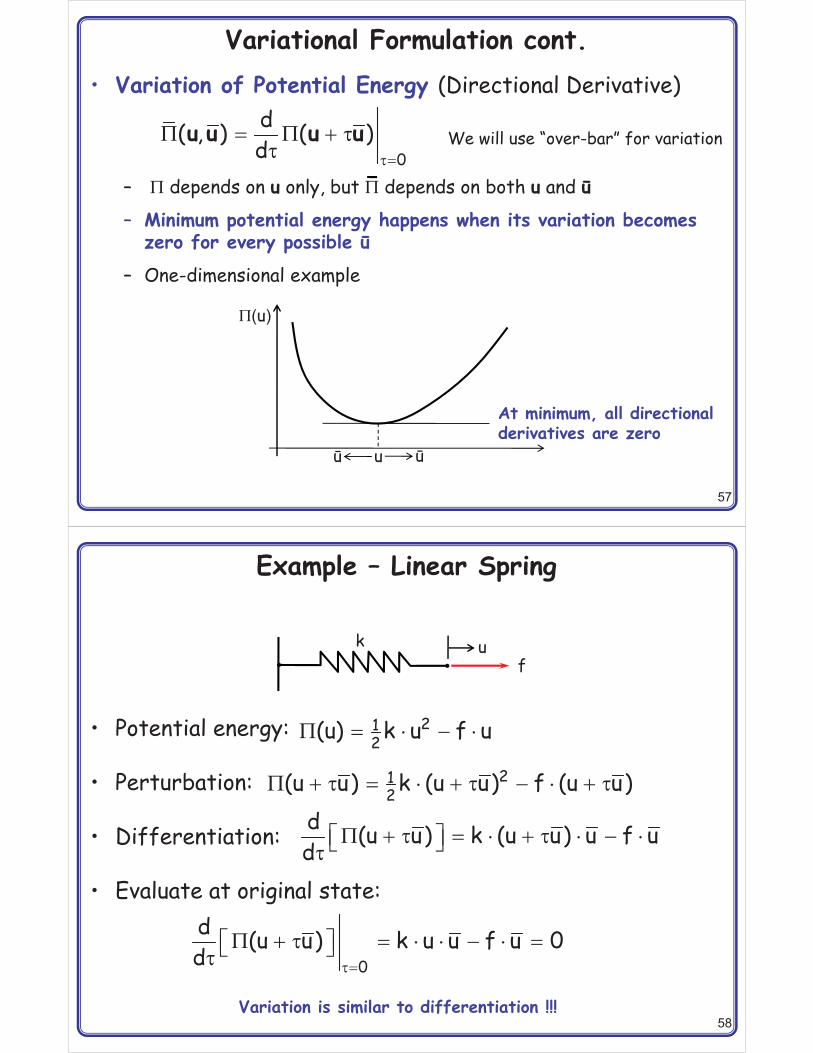
Variational Formulation cont.• Variation of Potential Energy (Directional Derivative)

– > depends on u only, but > depends on both u and �

– Minimum potential energy happens when its variation becomes zero for every possible �

– One-dimensional example

0

d( , ) ( )d 6�

> � > � 66

u u u u We will use “over-bar” for variation

>(u)

�u�

At minimum, all directional derivatives are zero

58

Example – Linear Spring

• Potential energy:

• Perturbation:

• Differentiation:

• Evaluate at original state:

212(u) k u f u> � & � &

212(u u) k (u u) f (u u)> � 6 � & � 6 � & � 6

d (u u) k (u u) u f ud

> � 6 � & � 6 & � &� �� 6

0

d (u u) k u u f u 0d 6�

> � 6 � & & � & �� 6

kf

u

Variation is similar to differentiation !!!

59

Variational Formulation cont.• Variational Equation

– From the definition of stress

– Note: load term is similar to linear problems

– Nonlinearity in the strain energy term

• Need to write LHS in terms of u and �

� � :

�> � � � � � : �

�22 22 2 s0 0 o

T b TW( )( , ) : d d d 0Eu u E u f u tE

for all � � �

s0 0 o

T b T: d d d� � :

� � � � :22 22 2S E u f u t

Variational equation in TL formulation

60

Variational Formulation cont.• How to express strain variation

� �T T1 10 0 0 02 2( ) ( )� � � � � E u C 1 u u u u

� ��

0T T T1

0 0 0 0 0 02T T1

0 0 0 02T T1

0 02

d( , ) ( )d

( ) ( )

6�

� � 66

� � � �

� � � �

� �

E u u E u u

u u u u u u

1 u u u 1 u

F u u F

T0( , ) sym( )� E u u u F

Note: E(u) is nonlinear, but is linear( , )E u u

61

Variational Formulation cont.• Variational Equation

• Linear in terms of strain if St. Venant-Kirchhoff material is used

• Also linear in terms of �• Nonlinear in terms of u because displacement-strain

relation is nonlinear

s0 0 o

T b T: d d d� � :

� � � � :22 22 2S E u f u t for all � � �

a( , )u u �( )u

Energy form Load form

a( , ) ( ),� 9 =u u u u ��

62

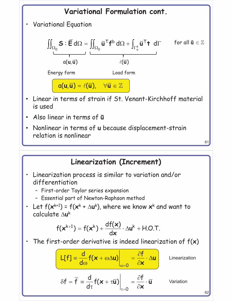
Linearization (Increment)• Linearization process is similar to variation and/or

differentiation– First-order Taylor series expansion– Essential part of Newton-Raphson method

• Let f(xk+1) = f(xk + 3uk), where we know xk and want to calculate 3uk

• The first-order derivative is indeed linearization of f(x)

� � � & 3 �k 1 k kdf( )f( ) f( ) H.O.T.dxx x ux

?�

� � ?3 � & 3

? �0

d fL[f] f( )d

x u ux

6�

�� 6 � &

6 �0

d ff f f( )d

x u ux

Linearization

Variation

63

Linearization of Residual• We are still in continuum domain (not discretized yet)• Residual• We want to linearize R(u) in the direction of 3u

– First, assume that u is perturbed in the direction of 3u using a variable 6. Then linearization becomes

– R(u) is nonlinear w.r.t. u, but L[R(u)] is linear w.r.t. 3u

– Iteration k did not converged, and we want to make the residual at iteration k+1 zero

R( ) a( , ) ( )� �u u u u�

T

0

R( ) RL[R( )]6�

� � 63 �� 3� ��6 ��

u uu uu

Tkk 1 k kR( )R( ) R( ) 0� � ��

� 3 � ��

uu u uu

64

Newton-Raphson Iteration by Linearization• This is N-R method (see Chapter 2)

• Update state

• We know how to calculate R(uk), but how about ?

– Only linearization of energy form will be required

– We will address displacement-dependent load later

Tkk kR( ) R( )

� ��3 � ��

u u uu

�

� �

� � 3

� �

k 1 k k

k 1 k 1u u ux X u

� ��

kR( )uu

[R( )] [a( , ) ( )]� ��

� �u u u u

u u�

xkxk+1 x3uk

f(xk)

f(xk+1)

��fx

65

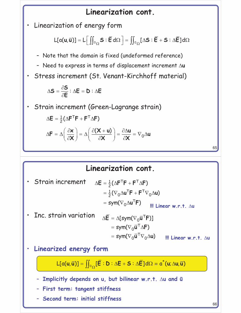
Linearization cont.• Linearization of energy form

– Note that the domain is fixed (undeformed reference)

– Need to express in terms of displacement increment 3u

• Stress increment (St. Venant-Kirchhoff material)

• Strain increment (Green-Lagrange strain)

� �� 3 � 3 �� 22 220 0L[a( , )] L : d [ : : ]du u S E S E S E

�3 � 3 � 3

�: :SS E D E

E

3 � 3 � 3T T12 ( )E F F F F

� � � �3� � � �3 � 3 � 3 � � 3� � � �� 0

( )x X u uF uX X X

66

Linearization cont.• Strain increment

• Inc. strain variation

• Linearized energy form

– Implicitly depends on u, but bilinear w.r.t. 3u and �

– First term: tangent stiffness

– Second term: initial stiffness

3 � 3 � 3

� 3 � 3

� 3

T T12

T T10 02

T0

( )

( )

sym( )

E F F F F

u F F u

u F !!! Linear w.r.t. 3u

3 � 3

� 3

� 3

T0T

0T

0 0

[sym( )]sym( )sym( )

E u Fu Fu u !!! Linear w.r.t. 3u

�� 3 � 3 � 3220 *L[a( , )] [ : : : ]d a ( ; , )u u E D E S E u u u

67

• N-R Iteration with Incremental Force– Let tn be the current load step and (k+1) be the current iteration

– Then, the N-R iteration can be done by

– Update the total displacement

• In discrete form

• What are and ?

Linearization cont.

3 � � 9 =�* n k k n ka ( ; , ) ( ) a( , ),u u u u u u u �

� � � 3n k 1 n k ku u u

3 �T n k k T n kT{ } [ ]{ } { } { }d K d d R

n kT[ ]K n k{ }R

68

Example – Uniaxial Bar• Kinematics

• Strain variation

• Strain energy density and stress

• Energy and load forms

• Variational equation

L0=1m

1 2F =�100N

x

� �2 2du duu , udX dX

� ��

22

11 2 2du 1 du 1E u (u )dX 2 dX 2

� & 2111 112W(E ) E (E ) � � �� & � ��

211 11 2 2

11

W 1S E E E u (u )E 2

� � � �11 2 2du du duE u (1 u )dX dX dX

� � �2 0L11 11 11 0 2 20

a(u,u) S E AdX S AL (1 u )u �� 2(u) u F

� �� 92 11 0 2 2R u S AL (1 u ) F 0, u

69

Example – Uniaxial Bar• Linearization

• N-R iteration

3 � 3 � � 311 11 2 2S E E E(1 u ) u 3 � 311 2 2E u u

� �3 � & & 3 � & 3

� � 3 � 3

2 0L*11 11 11 110

20 2 2 2 11 0 2 2

a (u; u,u) E E E S E AdX

EAL (1 u ) u u S AL u u

� � 3 � � �k 2 k k k k2 11 0 2 11 2 0[E(1 u ) S ]AL u F S (1 u )AL

� � � 3k 1 k k2 s 2u u u

70

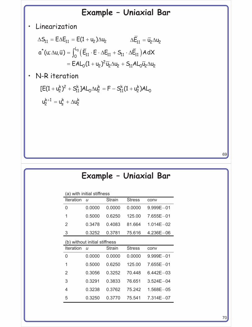
Example – Uniaxial Bar

(a) with initial stiffnessIteration u Strain Stress conv

0 0.0000 0.0000 0.0000 9.999E�01

1 0.5000 0.6250 125.00 7.655E�01

2 0.3478 0.4083 81.664 1.014E�02

3 0.3252 0.3781 75.616 4.236E�06

(b) without initial stiffnessIteration u Strain Stress conv

0 0.0000 0.0000 0.0000 9.999E�01

1 0.5000 0.6250 125.00 7.655E�01

2 0.3056 0.3252 70.448 6.442E�03

3 0.3291 0.3833 76.651 3.524E�04

4 0.3238 0.3762 75.242 1.568E�05

5 0.3250 0.3770 75.541 7.314E�07

71

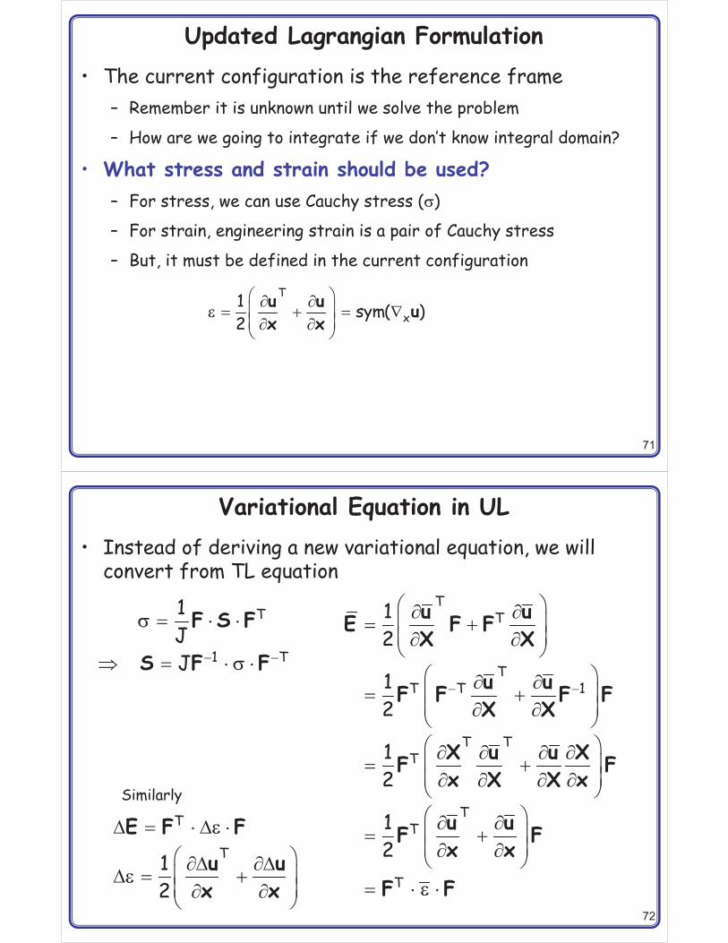
Updated Lagrangian Formulation• The current configuration is the reference frame

– Remember it is unknown until we solve the problem

– How are we going to integrate if we don’t know integral domain?

• What stress and strain should be used?– For stress, we can use Cauchy stress (5)

– For strain, engineering strain is a pair of Cauchy stress

– But, it must be defined in the current configuration

� ��

� ��

T

x1 sym( )2

u u ux x

�

72

Variational Equation in UL• Instead of deriving a new variational equation, we will

convert from TL equation

� �

� & &

� � & &

5

5

T

1 T

1JJ

F S F

S F F� �

� ��

� ��

� ��

� ��

� ��

� & &�

TT

TT T 1

T TT

TT

T

12

12

12

12

u uE F FX X

u uF F F FX X

X u u XF Fx X X x

u uF Fx x

F F

3 � & 3 &

� ��3 �33 � ��

� ��

�

�

T

T12

E F F

u ux x

Similarly

73

Variational Equation in UL cont.• Energy Form

– We just showed that material and spatial forms are mathematically equivalent

• Although they are equivalent, we use different notation:

• Variational Equation

� ��

� � � �22 22 5 �0 0

1 T Ta( , ) : d (J ) : ( )du u S E F F F F

� �5 � � � � 5 � � 5 �1 1ik kl jl mi mn nj mk nl kl mn mn mnF F F F

� � �� 22 22 22

0 0 x: d : Jd : dS E 5 � 5 �

�� 22 5 �

xa( , ) : du u

� 9 =�a( , ) ( ),u u u u � What happens to load form?

Is this linear or nonlinear?

74

@ 3kl( , )u u

Linearization of UL• Linearization of will be challenging because we

don’t know the current configuration (it is function of u)• Similar to the energy form, we can convert the linearized

energy form of TL• Remember• Initial stiffness term

xa ( , )u u

�3 � 3 � 3 �220* 0a ( ; , ) [ : : : ]du u u E D E S E

� �

� �

� �� 3 �3 �3 � ��

� �� 3 �3 �

� 5 �� 3 �3 ��

5 ��

5T T

1 T

m m m m1 1ik kl jl

i j i j

m m m mkl

k l k l

1: J( ) :2

u u u u1JF F2 X X X X

u u u u1J2 x x x x

u u u uS E F FX X X X

75

4th-order spatialconstitutive tensor

3 � & & & 3 &� � 3�

� �� 3��

� �T T

ki kl lj ijmn pm pq qn

kl ki lj ijmn pm qn pq

( : : ) ( ) : : ( )F F D F F

1J F F D F FJ

E D E F F D F F

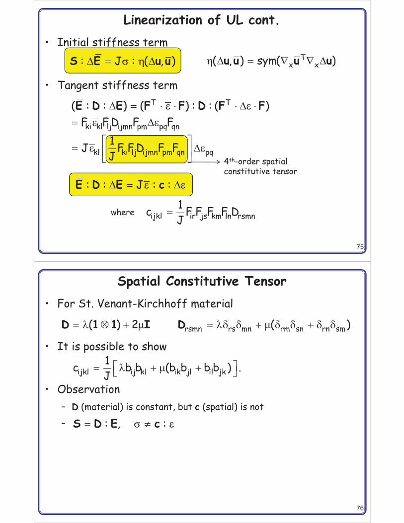
Linearization of UL cont.• Initial stiffness term

• Tangent stiffness term

3 � 35 @: J : ( , )S E u u 3 � 3@ Tx x( , ) sym( )u u u u

3 � 3� �: : J : :E D E c

where �ijkl ir js km ln rsmn1c F F F F DJ

76

Spatial Constitutive Tensor• For St. Venant-Kirchhoff material

• It is possible to show

• Observation– D (material) is constant, but c (spatial) is not

–

� * � 7 � � � � 7 � � � � �rsmn rs mn rm sn rn sm( ) 2 ( )D 1 1 I D

� �� 7 �� ijkl ij kl ik jl il jk1c b b (b b b b ) .J

� �5 �: , :S D E c

77

Linearization of UL cont.• From equivalence, the energy form is linearized in TL and

converted to UL

• N-R Iteration

• Observations– Two formulations are theoretically identical with different

expression

– Numerical implementation will be different

– Different constitutive relation

�� 3 � �22 � � 5 @

0L[a( , )] [ : : : ]Jdu u c

�3 � 3 � �22 � � 5 @

x

*a ( ; , ) [ : : : ]du u u c

3 � � 9 =�* n k k n ka ( ; , ) ( ) a( , ),u u u u u u u �

78

Example – Uniaxial Bar• Kinematics

• Deformation gradient:

• Cauchy stress:

• Strain variation:

• Energy & load forms:

• Residual:

L0=1m

1 2F =�100N

x� ��

2 2

2 2

u udu du,dx 1 u dx 1 u

� � � � �11 2 2dxF 1 u , J 1 udX

5 � � � �211 11 11 11 2 2 2

1 1F S F E(u u )(1 u )J 2

� ��

T 1 211 11 11 11

2

u(u) F E F1 u

� 5 � � 52L

11 11 11 20a(u,u) (u)Adx Au �� 2(u) u F

� �� 5 � � 92 11 2R u A F 0, u

79

Example – Uniaxial Bar• Spatial constitutive relation:

• Linearization:

� � � 31111 11 11 11 11 2

1c F F F F E (1 u ) EJ

� � 3 � � 32L 2

11 1111 11 2 2 20(u)c ( u)Adx EA(1 u ) u u

55 @ 3 � 3

�2L 11

11 11 2 20 2

A( u,u)Adx u u1 u

� �3 � � � 3 � 5 @ 3

5� � 3 � 3

�

2L*

11 1111 11 110

2 112 2 2 2 2

2

a (u; u,u) (u)c ( u) ( u,u) Adx

EA(1 u ) u u Au u1 u

Iteration u Strain Stress conv

0 0.0000 0.0000 0.000 9.999E�01

1 0.5000 0.3333 187.500 7.655E�01

2 0.3478 0.2581 110.068 1.014E�02

3 0.3252 0.2454 100.206 4.236E�06

80

Hyperelastic Material ModelSection 3.5

81

Goals• Understand the definition of hyperelastic material• Understand strain energy density function and how to use

it to obtain stress• Understand the role of invariants in hyperelasticity• Understand how to impose incompressibility• Understand mixed formulation and perturbed Lagrangian

formulation• Understand linearization process when strain energy

density is written in terms of invariants

82

What Is Hyperelasticity?• Hyperelastic material - stress-strain relationship derives

from a strain energy density function– Stress is a function of total strain (independent of history)

– Depending on strain energy density, different names are used, such as Mooney-Rivlin, Ogden, Yeoh, or polynomial model

• Generally comes with incompressibility (J = 1)– The volume preserves during large deformation

– Mixed formulation – completely incompressible hyperelasticity

– Penalty formulation - nearly incompressible hyperelasticity

• Example: rubber, biological tissues– nonlinear elastic, isotropic, incompressible and generally

independent of strain rate

• Hypoelastic material: relation is given in terms of stress and strain rates

83

Strain Energy Density• We are interested in isotropic materials

– Material frame indifference: no matter what coordinate system is chosen, the response of the material is identical

– The components of a deformation tensor depends on coord. system

– Three invariants of C are independent of coord. system

• Invariants of C

– In order to be material frame indifferent, material properties must be expressed using invariants

– For incompressibility, I3 = 1

� � � � � � � 2 2 21 11 22 33 1 2 3I tr( ) C C CC

� �� 2 2 2 2 2 2 2 21

2 1 2 2 3 3 12I (tr ) tr( )C C

� � 2 2 23 1 2 3I detC

No deformationI1 = 3I2 = 3I3 = 1

84

Strain Energy Density cont.• Strain Energy Density Function

– Must be zero when C = 1, i.e., 1 = 2 = 3 = 1

– For incompressible material

– Ex: Neo-Hookean model

– Mooney-Rivlin model

A

� � �� % m n k

1 2 3 mnk 1 2 3m n k 1

W(I ,I ,I ) A (I 3) (I 3) (I 1)

A

� �� % m n

1 2 mn 1 2m n 1

W(I ,I ) A (I 3) (I 3)

� �1 10 1W(I ) A (I 3)

� � � �1 2 10 1 01 2W(I ,I ) A (I 3) A (I 3)

7�10A

2

85

Strain Energy Density cont.• Strain Energy Density Function

– Yeoh model

– Ogden model

– When N = 1 and a1 = 1, Neo-Hookean material– When N = 2, 1 = 2, and 2 = �2, Mooney-Rivlin material

� � � � � �2 31 1 10 1 20 1 30 1W(I ) A (I 3) A (I 3) A (I 3)

� �

�

7 � � � �

%i i i

Ni

1 1 2 3 1 2 3i 1 i

W ( , , ) 3�

7 � 7%N

i ii 1

12

Initial shear modulus

86

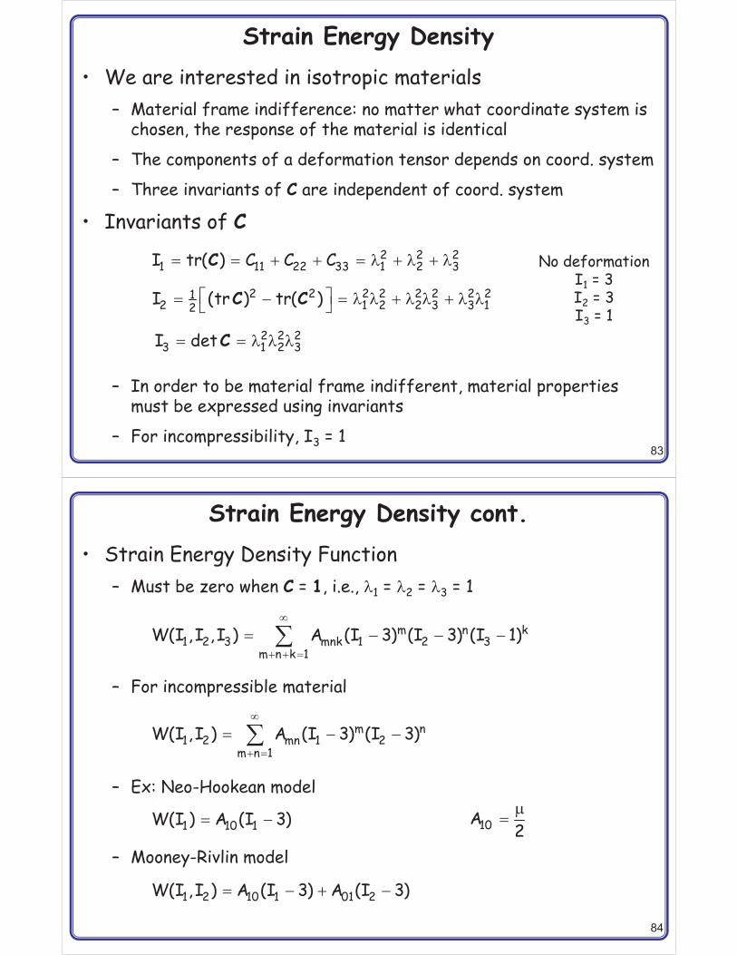
Example – Neo-Hookean Model• Uniaxial tension with incompressibility

• Energy density

• Nominal stress

� � � 1 2 3 1 /

� � � � � � � � �

2 2 2 210 1 10 1 2 3 10

2W A (I 3) A ( 3) A ( 3)

� �� 7 � � �� 10 2 2

W 1 1P 2A 1(1 )

-0.8 -0.4 0 0.4 0.8-250

-200

-150

-100

-50

0

50

Nominal strain

Nom

inal

stre

ss

Neo-Hookean

Linear elastic

87

Example – St. Venant Kirchhoff Material• Show that St. Venant-Kirchhoff material has the following

strain energy density

• First term

• Second term

� � 7� ��

2 2W( ) tr( ) tr( )2

E E E

��

�tr( )tr( ) : EE 1 E 1E

� � �� 7

� � �

2W( ) tr( ) tr( )tr( )E E ES EE E E

� � � *

�tr( )tr( ) ( : ) ( ) :EE 1 1 E 1 1 EE

��

�ij ji

ik jl ji ij jk il lk lk lkkl

E EE E E E 2E

E

88

Example – St. Venant Kirchhoff Material cont.• Therefore

� �� 7

� �� * � 7� * � 7� ��

2tr( ) tr( )tr( )

( ) : 2( ) 2 :

E ES EE E

1 1 E E1 1 I E

D

89

Nearly Incompressible Hyperelasticity• Incompressible material

– Cannot calculate stress from strain. Why?

• Nearly incompressible material– Many material show nearly incompressible behavior

– We can use the bulk modulus to model it

• Using I1 and I2 enough for incompressibility?– No, I1 and I2 actually vary under hydrostatic deformation

– We will use reduced invariants: J1, J2, and J3

• Will J1 and J2 be constant under dilatation?

� �� 1/3 2/3 1/21 1 3 2 2 3 3 3J I I J I I J J I

90

Locking• What is locking

– Elements do not want to deform even if forces are applied– Locking is one of the most common modes of failure in NL analysis– It is very difficult to find and solutions show strange behaviors

• Types of locking– Shear locking: shell or beam elements under transverse loading– Volumetric locking: large elastic and plastic deformation

• Why does locking occur?– Incompressible sphere under hydrostatic pressure

spherep

Volumetric strain

Pres

sure No unique pressure

for given displ.

91

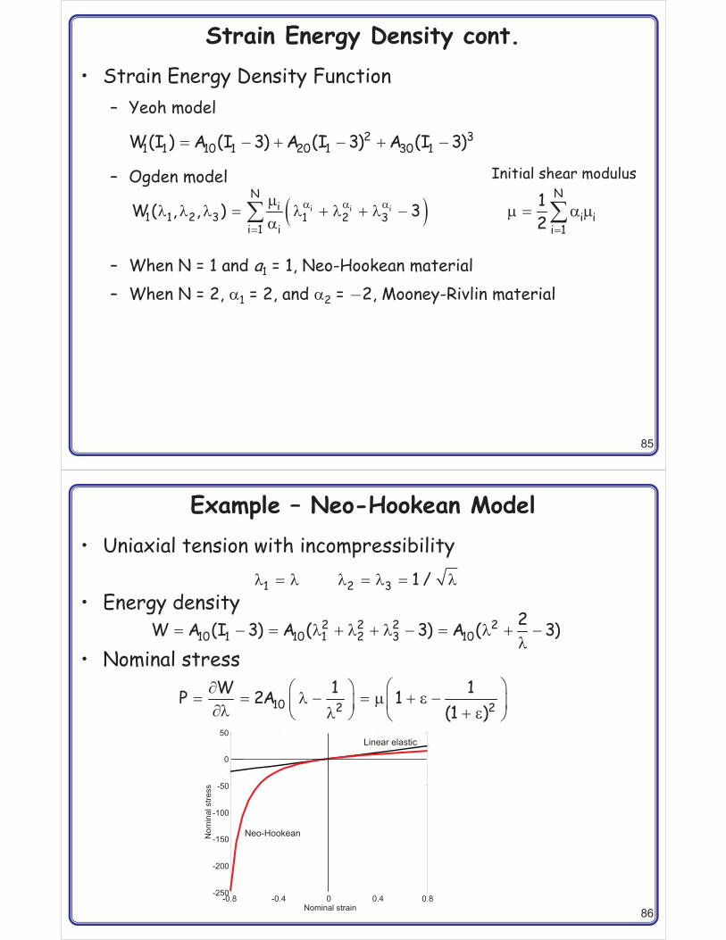
How to solve locking problems?• Mixed formulation (incompressibility)

– Can’t interpolate pressure from displacements

– Pressure should be considered as an independent variable

– Becomes the Lagrange multiplier method

– The stiffness matrix becomes positive semi-definite

4x1 formulation

Displacement

Pressure

92

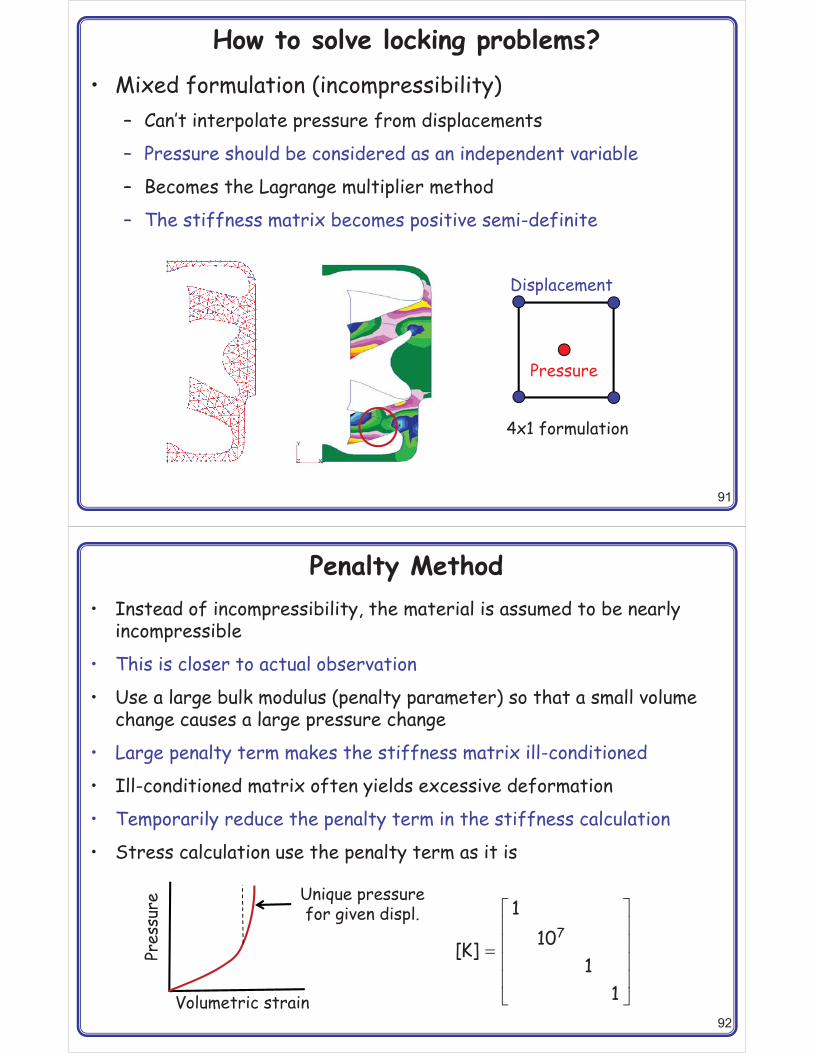
Penalty Method• Instead of incompressibility, the material is assumed to be nearly

incompressible

• This is closer to actual observation

• Use a large bulk modulus (penalty parameter) so that a small volume change causes a large pressure change

• Large penalty term makes the stiffness matrix ill-conditioned

• Ill-conditioned matrix often yields excessive deformation

• Temporarily reduce the penalty term in the stiffness calculation

• Stress calculation use the penalty term as it is

Volumetric strain

Pres

sure Unique pressure

for given displ.7

110[K]

11

� ��

93

Example – Hydrostatic Tension (Dilatation)

• Invariants

• Reduced invariants

� !" � #" � $

1 1

2 2

3 3

x Xx Xx X

� ��

0 00 00 0

F� � � �

� � ��

2

2

2

0 00 00 0

C

� � � 2 4 61 2 3I 3 I 3 I

�

�

� �

� �

� �

1/31 1 3

2/32 2 3

1/2 33 3

J I I 3J I I 3J I

I1 and I2 are not constant

J1 and J2 are constant

94

Strain Energy Density• Using reduced invariants

– WD(J1, J2): Distortional strain energy density

– WH(J3): Dilatational strain energy density

• The second terms is related to nearly incompressible behavior

– K: bulk modulus for linear elastic material

� �1 2 3 D 1 2 H 3W(J ,J ,J ) W (J ,J ) W (J )

� � 2H 3 3

KW (J ) (J 1)2� � 72

3

� � 2H 3 3

1W (J ) (J 1)2D

Abaqus:

95

Mooney-Rivlin Material• Most popular model

– (not because accuracy, but because convenience)

– Initial shear modulus ~ 2(A10 + A01)

– Initial Young’s modulus ~ 6(A10 + A01) (3D) or 8(A10 + A01) (2D)

– Bulk modulus = K

• Hydrostatic pressure

– Numerical instability for large K (volumetric locking)

– Penalty method with K as a penalty parameter

� �

� � � � � �

1 2 3 D 1 2 H 3

210 1 01 2 3

W(J ,J ,J ) W (J ,J ) W (J )KA (J 3) A (J 3) (J 1)2

��

H3

3 3

WWp K(J 1)J J

96

Mooney-Rivlin Material cont.• Second P-K stress

– Use chain rule of differentiation

��

� � � �

31 2

1 2 3

10 1, 01 2, 3 3,

JJ JW W W WJ J J

A J A J K(J 1)JE E E

SE E E E

S�

��,aaE E

� �

� �

�

� �

� �

�

1/3 4/311, 3 1, 1 3 3,3

2/3 5/322, 3 2, 2 3 3,3

1/213, 3 3,2

J (I )I I (I )I

J (I )I I (I )I

J (I )I

E E E

E E E

E E

�

� � �

� � � �

1,

2,9

3, imn jrs mr ns4

I 2I 4(1 tr ) 4I (2 4tr ) 4 [ e e E E ]

E

E

E

1E 1 EE 1 E

�

�

�

�

�

1/31 1 3

2/32 2 3

1/23 3

J I IJ I IJ I

�

�

� �

�

1,

2, 11

3, 3

I 2I 2(I )I 2I

E

E

E

11 CC

97

Example• Show• Let• Then• Derivatives

and

�� 11, 2, 1 3, 3I 2 , I 2(I ), I 2IE E E1 1 C C

� � �1 11 2 32 3I tr( ), I tr( ), I tr( )C CC CCC

� � � � � �2 31 11 1 2 1 2 3 3 1 1 22 6I I , I I I , I I I I I

��

� � �31 2

ij ji jk kiij ij ij

II I, C , C CC C C

��

� � �131 2

ij 1 ij ji 3 jiij ij ij

II I, I C , I CC C C

� ��

� �2

C E

98

Mixed Formulation• Using bulk modulus often causes instability

– Selectively reduced integration (Full integration for deviatoricpart, reduced integration for dilatation part)

• Mixed formulation: Independent treatment of pressure

– Pressure p is additional unknown (pure incompressible material)

– Advantage: No numerical instability

– Disadvantage: system matrix is not positive definite

• Perturbed Lagrangian formulation

– Second term make the material nearly incompressible and the system matrix positive definite

� �H 3 3W (J ,p) p(J 1)

� � � 2H 3 3

1W (J ,p) p(J 1) p2K

99

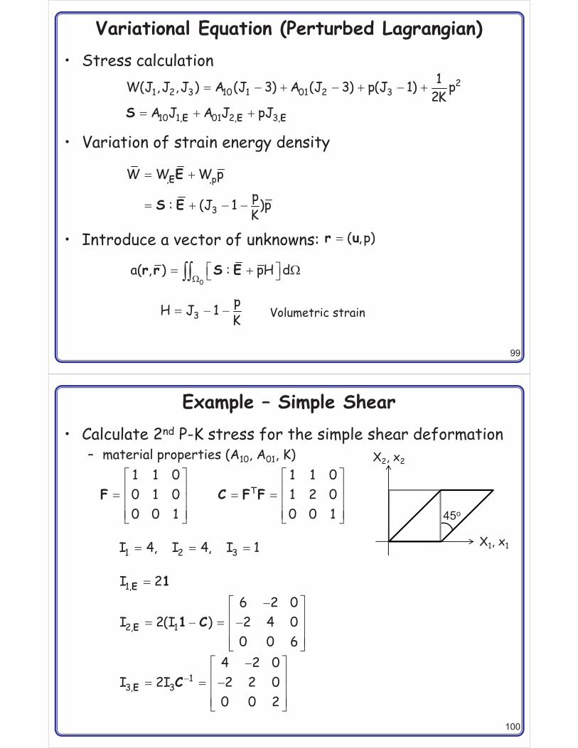
Variational Equation (Perturbed Lagrangian)• Stress calculation

• Variation of strain energy density

• Introduce a vector of unknowns:

� � �10 1, 01 2, 3,A J A J pJE E ES

� �

� � � �

, ,p

3

W W W pp: (J 1 )pK

EE

S E

� ( ,p)r u

�� 22

0a( , ) : pH dr r S E

� � �3pH J 1K Volumetric strain

� � � � � � � 21 2 3 10 1 01 2 3

1W(J ,J ,J ) A (J 3) A (J 3) p(J 1) p2K

100

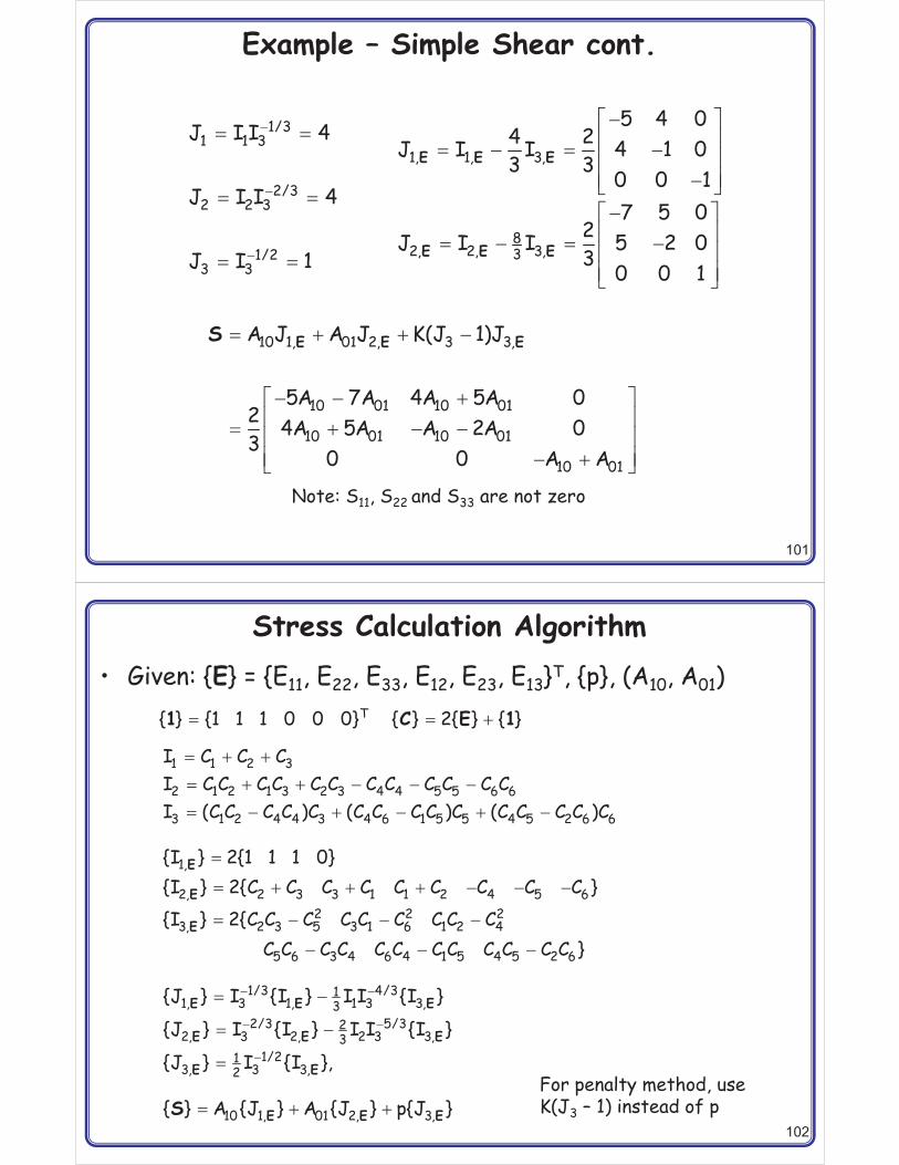
Example – Simple Shear• Calculate 2nd P-K stress for the simple shear deformation

– material properties (A10, A01, K)� � � ��

T1 1 0 1 1 00 1 0 1 2 00 0 1 0 0 1

F C F F

�

�

��

� ��

1,

2, 1

13, 3

I 26 2 0

I 2(I ) 2 4 00 0 6

4 2 0I 2I 2 2 0

0 0 2

E

E

E

1

1 C

C

X1, x1

X2, x2

45o

� � �1 2 3I 4, I 4, I 1

101

Example – Simple Shear cont.

��

1, 1, 3,

82, 2, 3,3

5 4 04 2J I I 4 1 03 3

0 0 17 5 0

2J I I 5 2 03

0 0 1

E E E

E E E

� � � �

� � ��

10 1, 01 2, 3 3,

10 01 10 01

10 01 10 01

10 01

A J A J K(J 1)J

5A 7A 4A 5A 02 4A 5A A 2A 03

0 0 A A

E E ES

Note: S11, S22 and S33 are not zero

�

�

�

� �

� �

� �

1/31 1 3

2/32 2 3

1/23 3

J I I 4

J I I 4

J I 1

102

Stress Calculation Algorithm• Given: {E} = {E11, E22, E33, E12, E23, E13}T, {p}, (A10, A01)

� � �T{ } {1 1 1 0 0 0} { } 2{ } { }1 C E 1

� � ��

1 1 2 3

2 1 2 1 3 2 3 4 4 5 5 6 6

3 1 2 4 4 3 4 6 1 5 5 4 5 2 6 6

I C C CI C C C C C C C C C C C CI (C C C C )C (C C C C )C (C C C C )C

�

� � � � � � �

� � � �

� � �

1,

2, 2 3 3 1 1 2 4 5 62 2 2

3, 2 3 5 3 1 6 1 2 4

5 6 3 4 6 4 1 5 4 5 2 6

{I } 2{1 1 1 0}{I } 2{C C C C C C C C C }{I } 2{C C C C C C C C C

C C C C C C C C C C C C }

E

E

E

� �

� �

�

� �

� �

�

1/3 4/311, 3 1, 1 3 3,3

2/3 5/322, 3 2, 2 3 3,3

1/213, 3 3,2

{J } I {I } I I {I }

{J } I {I } I I {I }

{J } I {I },

E E E

E E E

E E

� � �10 1, 01 2, 3,{ } A {J } A {J } p{J }E E ESFor penalty method, useK(J3 – 1) instead of p

103

Linearization (Penalty Method)• Stress increment

• Material stiffness

• Linearized energy form

�� 3 � 3 � 3 �� 22

0

*a ( ; , ) : : : du u u E D E S E

3 � 3 � 3, ,W : :E ES E D E

�� *� 10 1, 01 2, 3 3, 3, 3,A J A J K(J 1)J KJ JEE EE EE E ESDE

104

Linearization cont.• Second-order derivatives of reduced invariants

� � � �

� � � �

� �

� � * � * � * �

� � * � * � * �

� � * �

4 7 413 3 3 3

5 8 523 3 3 3

3 12 2

1, 1, 1, 3, 3, 1, 1 3, 3, 1 3,3 3 3 3

2, 2, 2, 3, 3, 2, 2 3, 3, 2 3,3 3 3 3

3, 3, 3, 3,3 3

1 4 1J I I I (I I I I ) I I I I I I I3 9 32 10 2J I I I (I I I I ) I I I I I I I3 9 3

1 1J I I I I I4 2

EE EE E E E E E E EE

EE EE E E E E E E EE

EE E E EE

� � � �

�

� * �

� * �

1,

2,1 1 1 1

3, 3 3

II 4I 4I I

EE

EE

EE

01 1 I

C C C IC

105

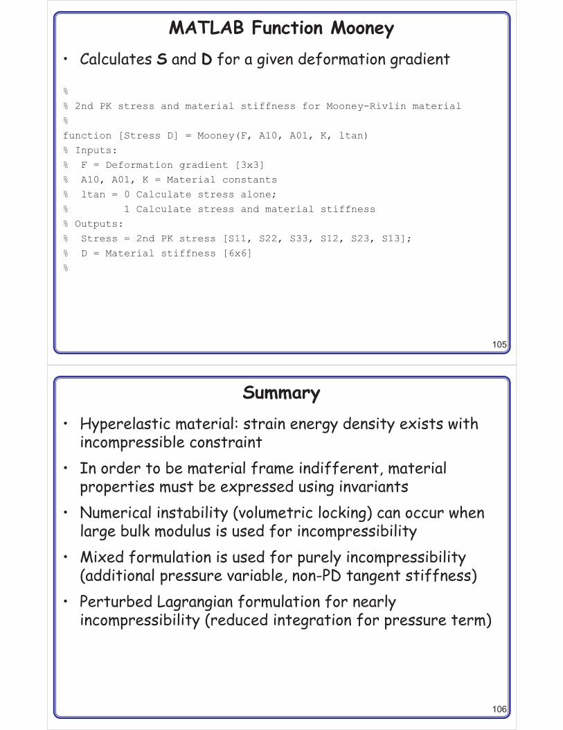
MATLAB Function Mooney• Calculates S and D for a given deformation gradient

%

% 2nd PK stress and material stiffness for Mooney-Rivlin material

%

function [Stress D] = Mooney(F, A10, A01, K, ltan)

% Inputs:

% F = Deformation gradient [3x3]

% A10, A01, K = Material constants

% ltan = 0 Calculate stress alone;

% 1 Calculate stress and material stiffness

% Outputs:

% Stress = 2nd PK stress [S11, S22, S33, S12, S23, S13];

% D = Material stiffness [6x6]

%

106

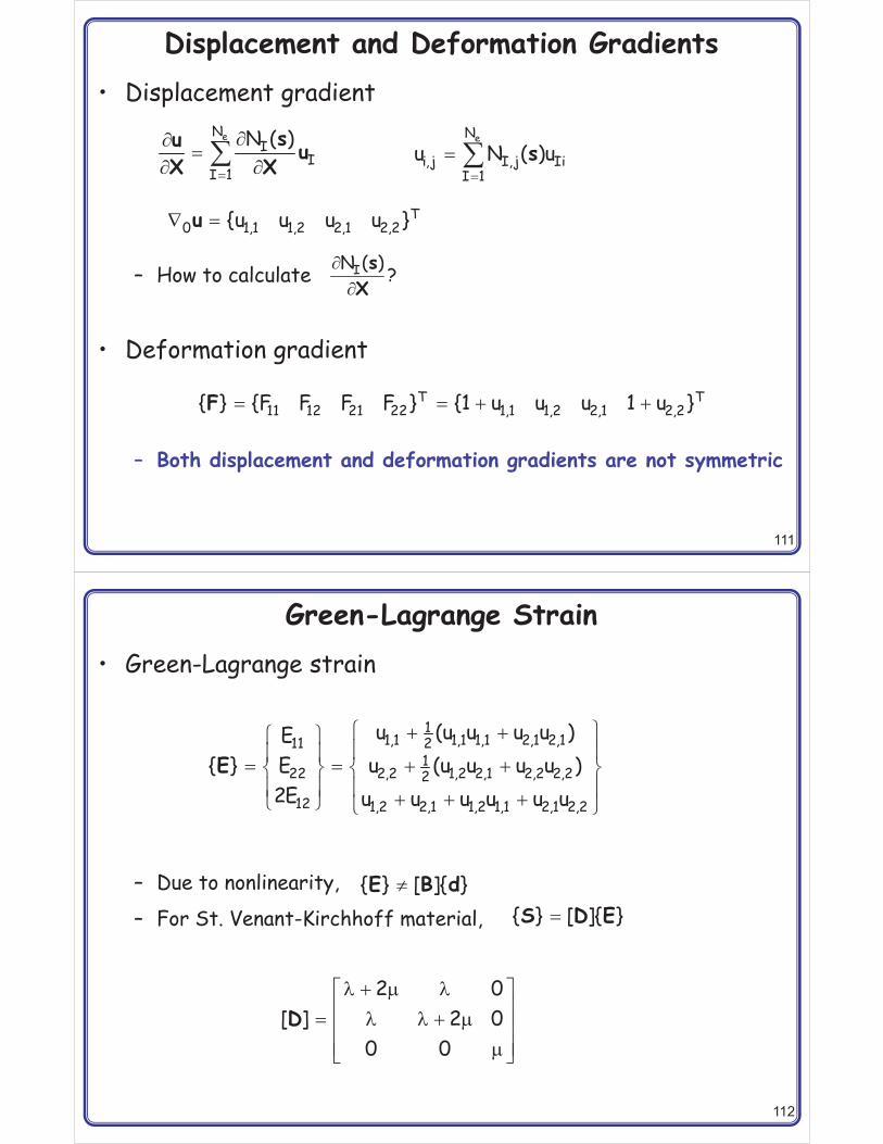
Summary• Hyperelastic material: strain energy density exists with

incompressible constraint• In order to be material frame indifferent, material

properties must be expressed using invariants• Numerical instability (volumetric locking) can occur when

large bulk modulus is used for incompressibility• Mixed formulation is used for purely incompressibility

(additional pressure variable, non-PD tangent stiffness)• Perturbed Lagrangian formulation for nearly

incompressibility (reduced integration for pressure term)

107

Finite Element Formulation for Nonlinear Elasticity

Section 3.6

108

Voigt Notation• We will use the Voigt notation because the tensor

notation is not convenient for implementation– 2nd-order tensor � vector– 4th-order tensor � matrix

• Stress and strain vectors (Voigt notation)

– Since stress and strain are symmetric, we don’t need 21 component

� T11 22 12{ } {E E 2E }E

� T11 22 12{ } {S S S }S

109

4-Node Quadrilateral Element in TL• We will use plane-strain, 4-node quadrilateral element to

discuss implementation of nonlinear elastic FEA• We will use TL formulation• UL formulation will be discussed in Chapter 4

Finite�Element�at�undeformed�domain

Reference�Element

X1

X2

1 2

34

s

t

(–1,–1) (1,–1)

(1,1)(–1,1)

110

Interpolation and Isoparametric Mapping• Displacement interpolation

• Isoparametric mapping– The same interpolation function is used for geometry mapping

�� %

eN

I II 1

N ( )u s u

�� %

eN

I II 1

N ( )X s X

Nodal displacement vector (uI, vI)

Interpolation function

Nodal coordinate (XI, YI)

� � �

� � �

� � �

� � �

11 4

12 4

13 4

14 4

N (1 s)(1 t)N (1 s)(1 t)N (1 s)(1 t)N (1 s)(1 t)

Interpolation (shape) function

• Same for all elements

• Mapping depends of geometry

111

Displacement and Deformation Gradients• Displacement gradient

– How to calculate


– Both displacement and deformation gradients are not symmetric

�

��

� �%eN

II

I 1

N ( )su uX X �

� %eN

i,j I,j IiI 1

u N ( )us

� T0 1,1 1,2 2,1 2,2{u u u u }u

� � � �T T11 12 21 22 1,1 1,2 2,1 2,2{ } {F F F F } {1 u u u 1 u }F

��IN ( ) ?sX

112

Green-Lagrange Strain• Green-Lagrange strain

– Due to nonlinearity,

– For St. Venant-Kirchhoff material,

! ,� �! ," "" "� � � �# - # -

" " " "� � �$ . $ .

11,1 1,1 1,1 2,1 2,1211

122 2,2 1,2 2,1 2,2 2,22

12 1,2 2,1 1,2 1,1 2,1 2,2

u (u u u u )E{ } E u (u u u u )

2E u u u u u uE

�{ } [ ]{ }E B d�{ } [ ]{ }S D E

� 7 � �� 7� �� 7� �

2 0[ ] 2 0

0 0D

113

Variation of G-R Strain• Although E(u) is nonlinear, is linear

� N{ } [ ]{ }E B d� T0( , ) sym( )E u u u F

( , )E u u

Function of uDifferent from linear strain-displacement matrix

� ��

�

�

�

11 1,1 21 1,1 11 2,1 21 2,1 11 4,1 21 4,1

N 12 1,2 22 1,2 12 2,2 22 2,2 12 4,2 22 4,2

11 1,2 21 1,2 11 2,2 21 2,2 11 4,2 21 4,2

12 1,1 22 1,1 12 2,1 22 2,1 12 4,1 22 4,1

F N F N F N F N F N F N

[ ] F N F N F N F N F N F N

F N F N F N F N F N F NF N F N F N F N F N F N

B

��

114

Variational Equation• Energy form

• Load form

• Residual

�

�

� �

� �

2222

0

0

T TN

T int

a( , ) : d

{ } [ ] { }d

{ } { }

u u S E

d B S

d F

; <� :

� :�

� � � :

� � � :

22 2

% 22 2

� S0 0

e

S0 0

T b T

NT bI I I

I 1T ext

( ) d d

N ( ) d N ( ) d

{ } { }

u u f u t

u s f s t

d F

� 9 = �T int T exth{ } { ( )} { } { }, { }d F d d F d

115

Linearization – Tangent Stiffness• Incremental strain • Linearization

3 � 3N{ } [ ]{ }E B d

� �� 3 � � � 3� �� 22 22

0 0

T TN N: : d { } [ ] [ ][ ]d { }E D E d B D B d

� �� 3 � � � 3� �� 22 22

0 0

T TG G: d { } [ ] [ ][ ]d { }S E d B B dB

� ��

11 12

12 22

11 12

12 22

S S 0 0S S 0 0[ ]0 0 S S0 0 S S

B

� ��

1,1 2,1 3,1 4,1

1,2 2,2 3,2 4,2G

1,1 2,1 3,1 4,1

2,1 2,2 3,2 4,2

N 0 N 0 N 0 N 0N 0 N 0 N 0 N 0

[ ]0 N 0 N 0 N 0 N0 N 0 N 0 N 0 N

B

116

Linearization – Tangent Stiffness• Tangent stiffness

• Discrete incremental equation (N-R iteration)

– [KT] changes according to stress and strain

– Solved iteratively until the residual term vanishes

�� 22 B

0

T TT N N G G 0[ ] [ ] [ ][ ] [ ] [ ][ ] dK B D B B B

3 � � 9 = �T T ext intT h{ } [ ]{ } { } { }, { }d K d d F F d

117

Summary• For elastic material, the variational equation can be

obtained from the principle of minimum potential energy• St. Venant-Kirchhoff material has linear relationship

between 2nd P-K stress and G-L strain• In TL, nonlinearity comes from nonlinear strain-

displacement relation• In UL, nonlinearity comes from constitutive relation and

unknown current domain (Jacobian of deformation gradient)

• TL and UL are mathematically equivalent, but have different reference frames

• TL and UL have different interpretation of constitutive relation.

118

MATLAB Code for Hyperelastic Material Model

Section 3.7

119

HYPER3D.m• Building the tangent stiffness matrix, [K], and the residual

force vector, {R}, for hyperelastic material

• Input variables for HYPER3D.mVariable Array size MeaningMID Integer Material Identification No. (3) (Not used)PROP (3,1) Material properties (A10, A01, K)UPDATE Logical variable If true, save stress valuesLTAN Logical variable If true, calculate the global stiffness matrixNE Integer Total number of elementsNDOF Integer Dimension of problem (3)XYZ (3,NNODE) Coordinates of all nodesLE (8,NE) Element connectivity

120

function HYPER3D(MID, PROP, UPDATE, LTAN, NE, NDOF, XYZ, LE)%***********************************************************************% MAIN PROGRAM COMPUTING GLOBAL STIFFNESS MATRIX AND RESIDUAL FORCE FOR% HYPERELASTIC MATERIAL MODELS%***********************************************************************%%

global DISPTD FORCE GKF SIGMA%% Integration points and weightsXG=[-0.57735026918963D0, 0.57735026918963D0];WGT=[1.00000000000000D0, 1.00000000000000D0];%% Index for history variables (each integration pt)INTN=0;%%LOOP OVER ELEMENTS, THIS IS MAIN LOOP TO COMPUTE K AND Ffor IE=1:NE

% Nodal coordinates and incremental displacementsELXY=XYZ(LE(IE,:),:);% Local to global mappingIDOF=zeros(1,24);for I=1:8

II=(I-1)*NDOF+1;IDOF(II:II+2)=(LE(IE,I)-1)*NDOF+1:(LE(IE,I)-1)*NDOF+3;

endDSP=DISPTD(IDOF);DSP=reshape(DSP,NDOF,8);

%%LOOP OVER INTEGRATION POINTSfor LX=1:2, for LY=1:2, for LZ=1:2

E1=XG(LX); E2=XG(LY); E3=XG(LZ);INTN = INTN + 1;%% Determinant and shape function derivatives[~, SHPD, DET] = SHAPEL([E1 E2 E3], ELXY);FAC=WGT(LX)*WGT(LY)*WGT(LZ)*DET;

121

% Deformation gradientF=DSP*SHPD' + eye(3);%% Computer stress and tangent stiffness[STRESS DTAN] = Mooney(F, PROP(1), PROP(2), PROP(3), LTAN);%% Store stress into the global arrayif UPDATE

SIGMA(:,INTN)=STRESS;continue;

end%% Add residual force and tangent stiffness matrixBM=zeros(6,24); BG=zeros(9,24);for I=1:8

COL=(I-1)*3+1:(I-1)*3+3;BM(:,COL)=[SHPD(1,I)*F(1,1) SHPD(1,I)*F(2,1) SHPD(1,I)*F(3,1);

SHPD(2,I)*F(1,2) SHPD(2,I)*F(2,2) SHPD(2,I)*F(3,2);SHPD(3,I)*F(1,3) SHPD(3,I)*F(2,3) SHPD(3,I)*F(3,3);SHPD(1,I)*F(1,2)+SHPD(2,I)*F(1,1)

SHPD(1,I)*F(2,2)+SHPD(2,I)*F(2,1) SHPD(1,I)*F(3,2)+SHPD(2,I)*F(3,1);SHPD(2,I)*F(1,3)+SHPD(3,I)*F(1,2)

SHPD(2,I)*F(2,3)+SHPD(3,I)*F(2,2) SHPD(2,I)*F(3,3)+SHPD(3,I)*F(3,2);SHPD(1,I)*F(1,3)+SHPD(3,I)*F(1,1)

SHPD(1,I)*F(2,3)+SHPD(3,I)*F(2,1) SHPD(1,I)*F(3,3)+SHPD(3,I)*F(3,1)];%BG(:,COL)=[SHPD(1,I) 0 0;

SHPD(2,I) 0 0;SHPD(3,I) 0 0;0 SHPD(1,I) 0;0 SHPD(2,I) 0;0 SHPD(3,I) 0;0 0 SHPD(1,I);0 0 SHPD(2,I);0 0 SHPD(3,I)];

end

122

%% Residual forcesFORCE(IDOF) = FORCE(IDOF) - FAC*BM'*STRESS;%% Tangent stiffnessif LTAN

SIG=[STRESS(1) STRESS(4) STRESS(6);STRESS(4) STRESS(2) STRESS(5);STRESS(6) STRESS(5) STRESS(3)];

SHEAD=zeros(9);SHEAD(1:3,1:3)=SIG;SHEAD(4:6,4:6)=SIG;SHEAD(7:9,7:9)=SIG;%EKF = BM'*DTAN*BM + BG'*SHEAD*BG;GKF(IDOF,IDOF)=GKF(IDOF,IDOF)+FAC*EKF;

endend; end; end;

endend

123

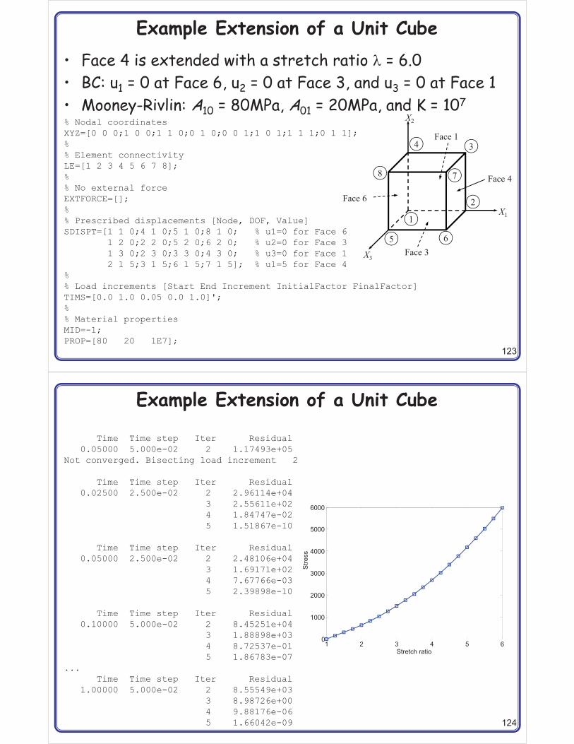
Example Extension of a Unit Cube• Face 4 is extended with a stretch ratio = 6.0• BC: u1 = 0 at Face 6, u2 = 0 at Face 3, and u3 = 0 at Face 1• Mooney-Rivlin: A10 = 80MPa, A01 = 20MPa, and K = 107

1

2

65

4 3

78

X1

X2

X3Face 3

Face 1

Face 4

Face 6

% Nodal coordinatesXYZ=[0 0 0;1 0 0;1 1 0;0 1 0;0 0 1;1 0 1;1 1 1;0 1 1];%% Element connectivityLE=[1 2 3 4 5 6 7 8];%% No external forceEXTFORCE=[];%% Prescribed displacements [Node, DOF, Value]SDISPT=[1 1 0;4 1 0;5 1 0;8 1 0; % u1=0 for Face 6

1 2 0;2 2 0;5 2 0;6 2 0; % u2=0 for Face 31 3 0;2 3 0;3 3 0;4 3 0; % u3=0 for Face 12 1 5;3 1 5;6 1 5;7 1 5]; % u1=5 for Face 4

%% Load increments [Start End Increment InitialFactor FinalFactor]TIMS=[0.0 1.0 0.05 0.0 1.0]';%% Material propertiesMID=-1;PROP=[80 20 1E7];

124

Example Extension of a Unit Cube

Time Time step Iter Residual 0.05000 5.000e-02 2 1.17493e+05

Not converged. Bisecting load increment 2


3 2.55611e+02 4 1.84747e-02 5 1.51867e-10


3 1.69171e+02 4 7.67766e-03 5 2.39898e-10


3 1.88898e+03 4 8.72537e-01 5 1.86783e-07

...Time Time step Iter Residual

1.00000 5.000e-02 2 8.55549e+03 3 8.98726e+00 4 9.88176e-06 5 1.66042e-09

1 2 3 4 5 60

1000

2000

3000

4000

5000

6000

Stretch ratio

Stre

ss

125

Hyperelastic Material Analysis Using ABAQUS• *ELEMENT,TYPE=C3D8RH,ELSET=ONE

– 8-node linear brick, reduced integration with hourglass control, hybrid with constant pressure

• *MATERIAL,NAME=MOONEY*HYPERELASTIC, MOONEY-RIVLIN80., 20.,– Mooney-Rivlin material with A10 = 80 and A01 = 20

• *STATIC,DIRECT– Fixed time step (no automatic time step control)

x

y

z

126

Hyperelastic Material Analysis Using ABAQUS*HEADING- Incompressible hyperelasticity (Mooney-

Rivlin) Uniaxial tension*NODE,NSET=ALL1,2,1.3,1.,1.,4,0.,1.,5,0.,0.,1.6,1.,0.,1.7,1.,1.,1.8,0.,1.,1.*NSET,NSET=FACE11,2,3,4*NSET,NSET=FACE31,2,5,6*NSET,NSET=FACE42,3,6,7*NSET,NSET=FACE64,1,8,5*ELEMENT,TYPE=C3D8RH,ELSET=ONE1,1,2,3,4,5,6,7,8*SOLID SECTION, ELSET=ONE,

MATERIAL= MOONEY

*MATERIAL,NAME=MOONEY*HYPERELASTIC, MOONEY-RIVLIN80., 20.,*STEP,NLGEOM,INC=20UNIAXIAL TENSION*STATIC,DIRECT1.,20.*BOUNDARY,OP=NEWFACE1,3FACE3,2FACE6,1FACE4,1,1,5.*EL PRINT,F=1S, E, *NODE PRINT,F=1U,RF*OUTPUT,FIELD,FREQ=1*ELEMENT OUTPUTS,E*OUTPUT,FIELD,FREQ=1*NODE OUTPUTU,RF*END STEP

127

Hyperelastic Material Analysis Using ABAQUS• Analytical solution procedure

– Gradually increase the principal stretch from 1 to 6– Deformation gradient

– Calculate J1,E and J2,E

– Calculate 2nd P-K stress

– Calculate Cauchy stress

– Remove the hydrostatic component of stress

� ��

� � ��

0 00 1 / 00 0 1 /

F

� �10 1, 01 2,A J A JE ES

� & & T1JF S F5

5 � 5 � 511 11 22

128

Hyperelastic Material Analysis Using ABAQUS• Comparison with analytical stress vs. numerical stress

129

Fitting Hyperelastic Material Parameters from Test Data

Section 3.9

130

Elastomer Test Procedures• Elastomer tests

– simple tension, simple compression, equi-biaxial tension, simple shear, pure shear, and volumetric compression

0 1 2 3 4 5 6 70

10

20

30

40

50

60

70

Nominal strain

Nom

inal

stre

ss

uni-axialbi-axialpure shear

131

FF L

Simple tension test

F

F

L

Pure shear test

L

F

Equal biaxial test

F

L

Volumetric compression test

Elastomer Tests• Data type: Nominal stress vs. principal stretch

132

Data Preparation• Need enough number of independent experimental data

– No rank deficiency for curve fitting algorithm• All tests measure principal stress and principle stretch

Experiment Type Stretch Stress

Uniaxial tension Stretch ratio '= L/L0 Nominal stress TE = F/A0

Equi-biaxialtension

Stretch ratio = L/L0 in y-direction

Nominal stress TE = F/A0in y-direction

Pure shear test Stretch ratio '= L/L0 Nominal stress TE = F/A0

Volumetric test Compression ratio '= L/L0 Pressure TE = F/A0

133

Data Preparation cont.• Uni-axial test

• Equi-biaxial test

• Pure shear test

� � � 1 2 3, 1 /

��

310 01

UT 2(1 )(A A )

� � ! ,� � � � � � # -� � $ .10T 2 3

10 0101

AT(A ,A , ) { } { } 2( ) 2(1 )

Ax b

� � � 21 2 3, 1 /

��

� 5 2

10 011 UT 2( )(A A )2

� � � 1 2 3, 1, 1 /

��

310 01

UT 2( )(A A )

134

Data Preparation cont.• Data Preparation

• For Mooney-Rivlin material model, nominal stress is a linear function of material parameters (A10, A01)

�

�

� �

� ��

1 2 3 i i 1 NDTE E E E E E E

1 2 3 i i 1 NDT

Type 1 1 1 4 4 4

T T T T T T T

135

Curve Fitting for Mooney-Rivlin Material• Need to determine A10 and A01 by minimizing error

between test data and model

• For Mooney-Rivlin, T(A10, A01, k) is linear function– Least-squares can be used

� ��

� %10 01

NDT 2Ek 10 01 kA ,A k 1

minimize T T(A ,A , )

� � ! ,� �" " " " � �� # - � �" " � �" " � �$ . � �

� �

T11

T2 1

TNDT NDT

( )TT ( ){ } { } [ ]{ }

T ( )

xxT b X b

x

! ,� # -$ .

10

01

A{ }

Ab

! ," "" "� # -" "" "$ .

�

E1E

E 2

ENDT

TT{ }

T

T

136

Curve Fitting cont.• Minimize error(square)

• Minimization � Linear regression equation

� � �

� � �

� � �

T E T E

E T E

E T E T T E T T

{ } { } { } { }{ } { }{ } { } 2{ } [ ] { } { } [ ] [ ]{ }

e e T T T TT Xb T XbT T b X T b X X b

�T T E[ ] [ ]{ } [ ] { }X X b X T

137

Stability of Constitutive Model• Stable material: the slope in the stress-strain curve is

always positive (Drucker stability)• Stability requirement (Mooney-Rivlin material)

• Stability check is normally performed at several specified deformations (principal directions)

• In order to be P.D.

�� d : : d 0D

5 � � 5 � �1 1 2 2d d d d 0

; < �� ! ,� � �# -� � �� $ .

11 12 11 2

21 22 2

D D dd d 0D D d

� ��

11 22

11 22 12 21

D D 0D D D D 0

chap 3 fea for nonlinear elastic problems - uf mae · 1 chap 3 fea for nonlinear elastic problems...

Documents