Union College Union College

Union | Digital Works Union | Digital Works

Honors Theses Student Work

5-2021

Chaos-Based Coffee Can Radar System Chaos-Based Coffee Can Radar System

Conor Willsie

Rong Chen Union College - Schenectady, NY

Follow this and additional works at: https://digitalworks.union.edu/theses

Part of the Signal Processing Commons, and the Systems and Communications Commons

Recommended Citation Recommended Citation Willsie, Conor and Chen, Rong, "Chaos-Based Coffee Can Radar System" (2021). Honors Theses. 2407. https://digitalworks.union.edu/theses/2407

This Open Access is brought to you for free and open access by the Student Work at Union | Digital Works. It has been accepted for inclusion in Honors Theses by an authorized administrator of Union | Digital Works. For more information, please contact digitalworks@union.edu.

Chaos-Based Coffee Can Radar System

Conor Willsie

ECE 499 - Electrical Engineering Capstone 3

Advisors: Dr. Chandra Pappu and Dr. James Silva

3/24/21

1

Abstract

Linear frequency modulated (LFM) radar systems are simple and easy to implement,

making them ideal for inexpensive undergraduate research projects. Unfortunately, LFM radar

schemes have multiple limitations that make them unviable in many real-world applications.

Given the limitations of LFM radar systems, we propose a chaos-based frequency modulated

(CBFM) system. In this paper, we present the theory, design, and experimental verification of a

CBFM radar system that has both ranging and synthetic aperture radar imaging capabilities. The

performance of our CBFM system is compared to that of the LFM system designed by MIT. We

document many challenges and unforeseen obstacles that were encountered while developing

one of the first CBFM radar systems. Although our initial results look promising, particularly for

ranging, there remains a significant amount of research and development to be done on the SAR

imaging signal processing software algorithms before a CBFM radar scheme is fully functional.

2

Acknowledgments

I would like to thank my partner, Rong Chen, for her outstanding effort on this project;

none of this would have been possible without her. I would also like to thank our advisors, Dr.

Chandra Pappu and Dr. James Silva, for being incredible mentors and using their experience and

expertise to guide us through this challenging 9-month project.

3

Table of Contents

Abstract ........................................................................................................................................... 1

Acknowledgments........................................................................................................................... 2

List of Figures ................................................................................................................................. 5

Introduction ..................................................................................................................................... 6

Problem Statement ...................................................................................................................... 7

Approach ..................................................................................................................................... 7

Project Goal ................................................................................................................................ 8

Background ..................................................................................................................................... 8

Project Origin .............................................................................................................................. 8

Chaos Theory .............................................................................................................................. 9

Quasi-LFM ................................................................................................................................ 11

Synthetic Aperture Radar (SAR) .............................................................................................. 11

Design Considerations .................................................................................................................. 13

Materials ................................................................................................................................... 13

Economics ................................................................................................................................. 13

Energy ....................................................................................................................................... 13

Environment .............................................................................................................................. 14

Ergonomics ............................................................................................................................... 14

Safety ........................................................................................................................................ 14

Legal ......................................................................................................................................... 14

Ethics......................................................................................................................................... 15

Design Requirements .................................................................................................................... 15

Design Alternatives ....................................................................................................................... 16

Modulation: Vtune ...................................................................................................................... 16

Signal Generation...................................................................................................................... 17

AM vs. FM ................................................................................................................................ 17

Design ........................................................................................................................................... 18

System Overview ...................................................................................................................... 18

Circuit-Generated Waveforms .................................................................................................. 19

MATLAB-Generated Signals: Periodic Chaos ......................................................................... 21

Compression Factor and Sensitivity Analysis .......................................................................... 23

4

Frequency Modulation .............................................................................................................. 24

Design Verification via Spectral Analysis ................................................................................ 27

Physical System Layout ............................................................................................................ 29

SAR Methodology and Software .............................................................................................. 29

Ranging Methodology .............................................................................................................. 32

Results ........................................................................................................................................... 32

Initial SAR Results ................................................................................................................... 32

SAR Problems ........................................................................................................................... 34

Ranging ..................................................................................................................................... 36

Troubleshooting Issues with CBFM for Ranging ..................................................................... 37

MATLAB-Generated Signal Results ........................................................................................ 39

Future Work .................................................................................................................................. 42

Conclusion .................................................................................................................................... 43

References ..................................................................................................................................... 44

Appendices .................................................................................................................................... 45

Appendix A. Complete Parts List and Funding Requested ...................................................... 45

Appendix B. Standards ............................................................................................................. 46

5

List of Figures Figure 1. Basic Radar System Block Diagram ............................................................................... 6

Figure 2. Lorenz oscillator x and y-state variables ....................................................................... 10

Figure 3. x vs. y-state "Owl's Face" Attractor Plot ....................................................................... 10

Figure 4. Segments of the Spectrogram of a Lorenz FM Signal with Positive Chirp Rates

(courtesy of [7]) ............................................................................................................................ 11

Figure 5. Synthetic aperture radar modes (courtesy of [8]) .......................................................... 12

Figure 6. Full Radar System Block Diagram ................................................................................ 18

Figure 7. Linear Ramp Generator Circuit ..................................................................................... 20

Figure 8. Linear Ramp Signal ....................................................................................................... 20

Figure 9. Lorenz Chaotic Oscillator Multisim Circuit Schematic Diagram ................................. 21

Figure 10. MATLAB-generated linear ramp signal ..................................................................... 22

Figure 11. MATLAB-generated quasi-LFM periodic chaos signal (C = 10-3.05) ......................... 22

Figure 12. Voltage Follower Circuit Schematic ........................................................................... 23

Figure 13. Periodic Chaos with Four Different Compression Factors.......................................... 24

Figure 14. FM Signal from VCO .................................................................................................. 26

Figure 15. Span (a) and Bias (b) Circuit Schematics .................................................................... 26

Figure 16. Raw Vtune (red) vs. Biased and Spanned Vtune (blue) .................................................. 27

Figure 17. Spectrum of LFM waveform ....................................................................................... 28

Figure 18. Spectrum of CBFM Waveform ................................................................................... 28

Figure 19. Complete radar system ................................................................................................ 29

Figure 20. SAR Data Collection Method (courtesy of [5]) .......................................................... 30

Figure 21. RMA Block Diagram (courtesy of [8]) ....................................................................... 31

Figure 22. RMA Range Parameter Geometry (courtesy of [8]) ................................................... 31

Figure 23. Steinmetz Car using LFM ........................................................................................... 33

Figure 24. Steinmetz Car using CBFM......................................................................................... 33

Figure 25. SAR Image Overlaid with Satellite Image .................................................................. 34

Figure 26. Chaotic Behavior of Center Frequency of CBFM Waveforms ................................... 35

Figure 27. Frequency-Time Plot of CBFM Waveform ................................................................ 35

Figure 28. Circuit-Generated RTI Plots ........................................................................................ 36

Figure 29. Range-time intensity algorithm diagram (LFM) ......................................................... 38

Figure 30. Range-time intensity algorithm diagram (CBFM) ...................................................... 38

Figure 31. MATLAB-generated LFM RTI plot ........................................................................... 39

Figure 32. Ranging Sensitivity Study ........................................................................................... 40

Figure 33. SAR Sensitivity Study ................................................................................................. 41

6

Introduction

Radio detection and ranging (radar) was first invented in England in 1935 by Sir Robert

Watson-Watt to detect enemy ships and aircraft during the impending world war [1]. The use of

radar technology has since spread far beyond the military, as it is currently used for air traffic

control, law enforcement, automotive cruise-control systems, and weather prediction. Radar

systems consist of four basic components: a waveform generator, a transmitter, a receiver, and a

processor. They work by transmitting radio frequency (RF) electromagnetic waves towards an

intended target. The receiver detects reflections, or “echoes”, as the RF waves bounce off the

target or any other objects in their path. The processor analyzes the signals from the receiver to

provide the user with information about the location and movement of the target [2]. A block

diagram of such a radar system is shown below in Figure 1:

Figure 1. Basic Radar System Block Diagram

The information from the signal processor is useful for a multitude of applications. Police

need this information to enforce speed limits. Aircraft pilots and ship captains use this

information to navigate through low-visibility environments. Modern cars use information from

built-in radar systems to autonomously slow down, speed up, or stop. Radar affects the lives of

millions of people every day, making it an important area of study. Fortunately, the open-source

7

coffee can radar system developed at MIT has helped make the study of radar more accessible to

undergraduates and it has established a good foundation for future iterations, such as the one

discussed in this paper [3].

Problem Statement

Low-cost radar systems, such as the one developed in the MIT open-source project,

typically transmit linear frequency modulated (LFM) signals. There are two principal issues

related to the use of LFM schemes in radar. First, these signals can be easily detected and

demodulated, which is not desirable in applications where security is important. Second, the

LFM-based radar system suffers from mutual interference issues when it is used in a crowded

environment [4]. For example, when there are multiple vehicles next to each other on the

highway using radar-based cruise control, the reliability of these safety features can be

compromised [4].

Approach

Based on these deficiencies, it is proposed to utilize chaotic waveforms rather than LFM

waveforms. Chaotic signals appear just like noise, yet they are completely deterministic.

Compared to a periodic RF signal such as FMCW1, a chaotic signal is much harder to distinguish

from noise. Even if detected, a chaotic signal would be difficult for an enemy to interpret and

replicate, thus making a counterattack unlikely. At the same time, the unique nature of solvable

chaos-based signals makes it possible to optimize their detection in an environment full of

1 FMCW: Frequency Modulated Continuous Wave is a waveform in which the frequency is modulated in a repeated

pattern, typically as a triangle or sinusoidal wave.

8

interference [4]. Incorporating chaos into a radar system would thus make it a much more viable

option for real-world use.

Project Goal

The goal of this project is to design, build, and test a functioning evolution of the coffee

can radar system originally designed by MIT that utilizes CBFM waveforms instead of LFM

waveforms. The proposed system would ideally have the same functionality as the MIT system,

namely, the ability to extract range and velocity information from targets, as well as capturing

synthetic aperture radar (SAR) imagery of targets. SAR imaging will be the focus of our

experimentation and will be discussed in detail in the background section of this report. More

specifically, we will compare the quality of SAR images obtained from LFM and CBFM

waveforms and identify issues with implementation of CBFM for SAR imaging. Ultimately, this

project should result in an inexpensive system that is robust enough to be used for years to come

by Union College’s Electrical Engineering department.

Background

Project Origin

This study is fundamentally based on the coffee can radar system proposed by MIT [5].

The LFM-based radar system in the MIT system has ranging, doppler, and SAR imaging

capabilities [5]. To alleviate the limitations associated with LFM waveforms, Beal et al.

proposed a modification of the MIT design that is based on a solvable chaotic waveform [4]. In

their paper, Beal at al. demonstrated one of the first chaos-based amplitude modulated (AM)

radar systems [4]. Regarding the incorporation of a chaotic oscillator into the MIT coffee can

radar, Beal’s paper serves as a proof of concept and gives a foundation for our work. Considering

the disadvantages such as non-constant envelope, spectral leakage, and limited bandwidth

9

optimization capabilities, we are approaching the problem using a frequency modulated (FM)

scheme instead.

Chaos Theory

The original design for a Lorenz chaotic oscillator circuit, shown in Figure 9 in the design

section, is discussed by P. Horowitz in [6]. This chaos for radar systems was used by A. N. Beal

et al. in [4]. and B. C. Flores et al. in [7]. Considering the simplicity of the Lorenz system and

inherent advantages it possesses, we utilize the Lorenz oscillator for our study’s purposes. A

physical system that generates chaotic voltage waveforms is modeled using a three-dimensional

nonlinear system of differential equations, as shown in equations 1-3.

x′ = σ(y − x)

y′ = x(ρ − z) – y

z′ = xy – βz

Equations 1-3. Lorenz Chaotic System of Differential Equations

The following values, 𝜎 = 10, ⍴ = 28, and β = 8/3, are typical choices for the parameters

that control the dynamics of this system [6]. These parameter values are intentionally chosen

such that the Lorenz system is chaotic [6]. The resistor values of the circuit realization of the

Lorenz oscillator are determined by the control parameter values of 𝜎, ⍴, and β [6].

The design of Lorenz chaotic circuit is based on the work of Harvard University’s

Professor Paul Horowitz [6]. For circuit implementation, inverting op-amps (LM741CN) with

feedback capacitors were used as integrators and summers to solve Equations 1-3. Analog

multipliers were used to create nonlinear products by multiplying the outputs of the op-amps.

From these op-amps, the Lorenz oscillator produced three chaotic state variables, x(t), y(t), and

z(t). The size of the feedback capacitors determined the system compression factor, and therefore

10

the frequency of the system’s oscillations. Figure 2 is an example output for the x and y-state

variables of the chaotic oscillator circuit.

Figure 2. Lorenz oscillator x and y-state variables

One can observe the aperiodic, bounded, and pseudo-random nature of these signals in

Figure 2. When x(t) is plotted against y(t), the characteristic Lorenz attractor is seen, also called

the “Butterfly Plot” or “Owl’s Face.” Securing a correct Lorenz attractor plot was a key step to

ensure that the chaotic oscillator was functioning properly. The Lorenz attractor is shown in

Figure 3.

Figure 3. x vs. y-state "Owl's Face" Attractor Plot

11

Since the op-amps and multipliers of our Lorenz oscillator required ±15V, we built our

circuit on a powered breadboard that supplied ±15V. The protoboard was powered with a

battery-powered power strip so our radar system remained mobile.

Quasi-LFM

As discussed later in the Results section, quasi-LFM signals became integral to our

success in creating a functional CBFM radar. Flores et al. discuss the generation of FM signals

that display quasi-chirp, or quasi-LFM, behavior using chaos in [7]. Using the Lorenz chaotic

system discussed above in the Chaos Theory section, Flores et al. produced ultra-wideband

chaotic FM signals that displayed positive chirping on a time-frequency plot, as shown in Figure

4 [7].

Figure 4. Segments of the Spectrogram of a Lorenz FM Signal with Positive Chirp Rates

(courtesy of [7])

Flores et al. propose that their approach could have the potential for anti-jamming

systems since the FM signals provide frequency agility that is not found in LFM or other pseudo-

random signals. This phenomenon is discussed further in the Results section.

Synthetic Aperture Radar (SAR)

W. G. Carrara et al. discussed the fundamentals of SAR imaging and the associated

signal processing algorithms [8]; this source was invaluable for our work. Synthetic aperture

12

radar was first developed in 1951 by Carl Wiley of the Goodyear Aircraft Corporation to

improve conventional imaging radar [8]. SAR uses the motion of the radar over a target region to

increase the apparent “aperture” or antenna diameter, which provides improved spatial resolution

of the target scene [8]. A practical means to move the radar to perform SAR imaging is to mount

it to a moving platform, such as an aircraft [8]. Figure 5 shows the three modes of SAR imaging:

spotlight, stripmap, and scan. We will be using stripmap mode, in which the radar is aimed in a

fixed direction and moved linearly across a target area that is parallel to the movement of the

radar system, shown in Figure 5.

Figure 5. Synthetic aperture radar modes (courtesy of [8])

SAR has been adapted to fit the needs of many different users and applications [8].

However, the possibility of day/night and all-weather operation is especially useful for the

military, where SAR imaging is used to perform weapons guidance and reconnaissance [8].

Examples of civilian applications include sea ice tracking, topographic mapping, and agricultural

assessment [8].

13

Design Considerations

Materials

For our radar system’s hardware, we will use inexpensive, low-power, commercial off-

the-shelf (COTS) components [4]. The core components of this project are two coffee cans,

which will be used as the transmitter and receiver antennas, a chaotic oscillator, and an ordinary

desktop or laptop computer for signal processing [4]. Other RF components include an

attenuator, amplifiers, splitters, and mixers.

Economics

The target cost of this radar system is $500 or less so that it may be replicated affordably

and be covered by a Union College Student Research Grant (SRG). A comprehensive parts list

can be found in Appendix A. To save money, we reused many of the components from a

capstone project conducted by two Union College class of 2020 electrical engineering students,

Kyle Meza and Dale Coker [9].

Energy

This radar system has a low energy requirement and can be powered by two 6V battery

packs using AA cells, according to the MIT design [5]. Although the Lorenz chaotic oscillator

power requirement is also low, it requires ±15VDC for three op-amps used to integrate the

differential equations. Rather than using additional batteries, the Lorenz oscillator utilizes a

powered breadboard, which is plugged into a rechargeable uninterruptible power supply for

portability. The power emitted by the radar system is within 20mW the norms set by the FCC for

the usage of systems in the ISM band.

14

Environment

The radar system will not have any negative impact on the environment due to the low

energy requirements and low power emission. The low power emission will ensure that no living

organisms near the testing location will be harmed by the EM radiation. Additionally, the raw

materials and circuit components used to construct the radar system will be reused by the ECE

department at Union College for many years.

Ergonomics

The ergonomics of our radar should reflect those of the original system built by MIT. The

entire radar system should be mobile enough for a single person to move, set up, and use around

Union’s campus with ease.

Safety

Our system must be safe for the user, targets, and bystanders. Therefore, the

electromagnetic (EM) waves that we transmit must not have adverse health effects for any living

organisms that may be in their path. Additionally, our radar system must not interfere with other

electromagnetic devices or communication systems. Therefore, our system operates under 20mW

total power.

Legal

Since this project is based on the information from an MIT OpenCourseWare project and

Beal’s work, the material for this project is also open-source [4], [5]. This project cannot be

claimed as intellectual property by myself or Union College.

15

Ethics

There are two main ethical considerations for our project. First, we must make sure to

credit the contributions of others on our radar system [10]. We must properly acknowledge the

professors at MIT who designed the original coffee can radar system. Like the MIT project, our

project will remain open-source and will never be used for commercial purposes. Similarly, we

must properly credit A. N. Beal et al. for the ideas we borrow from their work on a chaos-based

coffee can radar system. Their paper lays the groundwork for our project as we are trying to

replicate their results combined with MIT’s results. It is necessary to understand that our radar

system is being created purely to increase the understanding of such systems and raise interest in

radar and chaos.

Second, we must prioritize the health and safety of the public and quickly disclose

anything that may pose a threat to the public or the surrounding environment [10]. This is why it

will be important for us to closely follow the safety standards of OSHA in our radar design. It

will be our primary concern to ensure the electromagnetic radiation produced by our radar is well

within the proper operating conditions. Though we are confident in the safety of the work of

MIT and Audrey Beal et al., we will communicate any concerns we have in our design. More

details about the specific standards in play can be found in Appendix B.

Design Requirements

Our primary design requirements come from the original MIT design in addition to the

fact that we need to operate our radar within the portion of the frequency spectrum reserved for

industrial, scientific, and medical (ISM) purposes. To operate within our frequency allocation of

the ISM band, we have to carefully consult the datasheet of our voltage-controlled oscillator

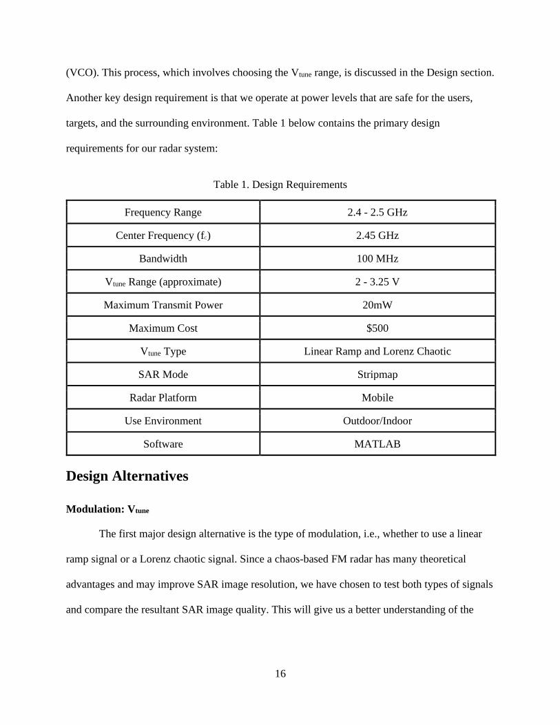
16

(VCO). This process, which involves choosing the Vtune range, is discussed in the Design section.

Another key design requirement is that we operate at power levels that are safe for the users,

targets, and the surrounding environment. Table 1 below contains the primary design

requirements for our radar system:

Table 1. Design Requirements

Frequency Range 2.4 - 2.5 GHz

Center Frequency (fC) 2.45 GHz

Bandwidth 100 MHz

Vtune Range (approximate) 2 - 3.25 V

Maximum Transmit Power 20mW

Maximum Cost $500

Vtune Type Linear Ramp and Lorenz Chaotic

SAR Mode Stripmap

Radar Platform Mobile

Use Environment Outdoor/Indoor

Software MATLAB

Design Alternatives

Modulation: Vtune

The first major design alternative is the type of modulation, i.e., whether to use a linear

ramp signal or a Lorenz chaotic signal. Since a chaos-based FM radar has many theoretical

advantages and may improve SAR image resolution, we have chosen to test both types of signals

and compare the resultant SAR image quality. This will give us a better understanding of the

17

advantages and disadvantages of each type of signal and enable interesting comparisons in our

Results section.

Signal Generation

The next design alternative was the use of circuit-generated signals vs. MATLAB-

generated signals. The MIT LFM radar and the Beal et al. chaos-based amplitude modulated

(CBAM) radar both used circuit-generated signals. The major disadvantage to this approach is

that a signal-producing circuit has little flexibility once it is built. To change its output, one needs

to create and implement a new design, which is very time-consuming. Alternatively, producing

signals in MATLAB is quite easy, especially if many adjustments are needed for testing

purposes. Although we began this project using circuit-generated signals, we transitioned to

MATLAB-generated signals to implement “periodic” non-linear signals, such as the quasi-LFM

chaos and non-linear FM signals discussed in the background section.

AM vs. FM

Lastly, we had to choose between amplitude and frequency modulation. Beal et al.

successfully used an AM scheme for their chaotic radar system [4]. They briefly mention that

FM schemes may provide favorable results, but they did not successfully implement an FM

scheme themselves [4]. Therefore, we will use a FM scheme in order to explore its possibilities

and because this relates more directly to the original MIT design. Further, Meza and Coker

already built an FM radar system using a VCO and it seemed logical to continue the work they

started [9].

18

Design

System Overview

This section of the paper covers the overall radar system design. We begin with a block

diagram of the entire system, shown in Figure 6:

Figure 6. Full Radar System Block Diagram

The components shaded in green are the areas of focus for this project and where most of

the work and experimentation was performed. The RF components shaded in blue, in addition to

the VCO, were shown to work in the radar previously built by Meza and Coker [9].

At the most basic level, this system produces a modulating waveform for the VCO that

yields a frequency-modulated signal in the frequency range of 2.4 - 2.5 GHz. This FM signal is

attenuated and amplified to obtain the desired amplitude, then split and transmitted towards a

target. In the presence of a target, the transmitted waveform gets reflected back and is captured

by the receiver. After passing through an RF amplifier, the received signal is mixed with the

transmitted signal to yield a waveform with two new frequencies: the sum and difference of the

transmitted and received frequencies, which are fed to a video amplifier and low-pass filter

(LPF). The video amplifier provides gain and the LPF removes the sum of the transmitted and

19

received frequencies. The remaining signal (at the difference between transmitted and received

frequencies) is in the audio frequency (AF) range. This signal is fed to the right channel of a

laptop’s audio input. The sync pulse, which is produced either by an on-board ramp generator or

by MATLAB, is fed into the left channel of the laptop’s audio input. These two AF signals,

recorded by Audacity® (a Windows or Macintosh App), comprise the radar data that is collected

when performing SAR imaging or ranging. After data collection is complete, the .wav file

generated by Audacity is imported into MATLAB for signal processing and SAR image or

range-time intensity (RTI) plot generation. An RTI plot indicates the intensity of the received

radar signal at the relative range from the antenna and time of the experiment.

Circuit-Generated Waveforms

There are two waveform generating circuits in our radar system, one produces a linear

ramp signal and the other produces a chaotic signal. The outputs of both of these waveform

generators will be called Vtune and will be used as the input for the VCO. First, we will discuss

the linear ramp signal generator. The linear ramp signal was produced using a monolithic

function generator chip (XR-2206). A circuit diagram of the linear ramp generator is shown in

Figure 7 and the output of this circuit is shown in Figure 8.

20

Figure 7. Linear Ramp Generator Circuit

Figure 8. Linear Ramp Signal

This chip also produces the sync pulse. Since this chip requires a +12V and +5V supply,

we utilized a +5V voltage regulator in addition to our two 6V battery packs, which produced an

unregulated +12V when connected in series.

21

The construction of the Lorenz chaotic oscillator circuit was a key step towards our goal

of developing a chaos-based radar system for SAR imaging. Figure 9 shows a schematic diagram

for the Lorenz oscillator.

Figure 9. Lorenz Chaotic Oscillator Multisim Circuit Schematic Diagram

MATLAB-Generated Signals: Periodic Chaos

To implement the quasi-LFM signals instead of aperiodic circuit-generated chaotic

signals from the Lorenz oscillator, we decided to use MATLAB. Once generated in the

MATLAB code, we could output the quasi-LFM signal through the laptop audio output jack to

the voltage-controlled oscillator (VCO), just as we did with the circuit-generated signals. Using

this method, we could essentially create a “periodic”, monotonically increasing chaos signal with

a fixed period of 40ms to match the base case LFM signal. Figure 10 shows our base case linear

ramp signal. Figure 11 shows our “periodic” chaos, or quasi-LFM signal.

22

Figure 10. MATLAB-generated linear ramp signal

Figure 11. MATLAB-generated quasi-LFM periodic chaos signal (C = 10-3.05)

To prevent the laptop audio input circuitry from loading the bias and span circuit, we

placed a voltage follower circuit with a gain of 1 between the bias and span circuit and the

laptop. This was necessary due to the low input impedance of the laptop audio input circuit,

which placed a load on the bias and span circuit. Once this buffer was installed, we were able to

use MATLAB-generated signals for our Vtune and sync pulse. A schematic of the simple voltage

follower is shown in Figure 12.

23

Figure 12. Voltage Follower Circuit Schematic

Compression Factor and Sensitivity Analysis

To slow down the oscillations of the Lorenz system to create a monotonically increasing

quasi-LFM signal, we had to adjust the compression factor (C value). The compression factor

controls the frequency of the chaotic system’s oscillations. The larger the compression factor, the

faster the oscillations. Since we want only a partial oscillation that approximates a linear ramp, a

lower compression factor is used. To observe the impact of the compression factor on the

resultant RTI and SAR images, we performed a sensitivity analysis by varying the compression

factor recording data for each waveform. Figure 13 shows four different chaos signals with four

different compression factors. The “chirp time” for each waveform is 20ms.

24

Figure 13. Periodic Chaos with Four Different Compression Factors

Figure 13a) is periodic chaos signal with a compression factor of C = 10-2.75. The

compression factor is increased in each plot, until a value of C = 10-2.00 is reached in Figure 13d).

The effects of compression factor on SAR imaging and ranging are discussed in the Results

section.

Frequency Modulation

For our radar system we use a voltage-controlled oscillator (VCO, Mini-Circuits ZX95-

2536C+) to produce FM waveforms. The VCO essentially maps the instantaneous value of Vtune

to a sine wave of a frequency proportional to Vtune, as shown in Table 2.

25

Table 2. Vtune vs. frequency for VCO

At 25oC, Table 2 shows that to maintain an output frequency between 2.4 and 2.5 GHz

(The ISM band), Vtune must stay between 2.00V and 3.25V. This Vtune range applies to both the

linear ramp and chaotic signals.

shows an example of the input and output of the VCO. The black waveform in

represents Vtune and the red waveform represents the VCO output signal. It is noted that

when the amplitude of Vtune increases, the frequency of the FM signal increases; when its

amplitude decreases, the frequency of FM waveform decreases.

26

Figure 14. FM Signal from VCO

To maintain the Vtune signal between 2.00V and 3.25V, we introduced a bias and span

circuit into each waveform generator using an op-amp (for bias) and a potentiometer (for span)

as shown in Figure 15.

Figure 15. Span (a) and Bias (b) Circuit Schematics

The function of the bias circuit is to add a DC bias to Vtune so that the center frequency of

our VCO output was 2.45 GHz. The function of the span circuit is to adjust the amplitude of

27

Vtune to the desired 2.00 - 3.25V range. Figure 16 shows the differences between an unbiased and

unscaled Vtune (red) and a biased and scaled Vtune (blue) for the chaotic oscillator.

Figure 16. Raw Vtune (red) vs. Biased and Spanned Vtune (blue)

Design Verification via Spectral Analysis

To ensure that our transmitted signal from the VCO output was operating within our

desired ISM band, we needed to measure the frequency content of the VCO output. We used a

Tektronix RSA518A real-time spectrum analyzer to accurately make this measurement. The

spectrum analyzer is able to display various types of information about our transmitted signal in

the frequency domain. Figure 17 shows the frequency spectrum of our VCO output using the

linear ramp signal as Vtune (LFM); Figure 18 shows the frequency spectrum of our VCO output

using the x(t) output of the chaotic oscillator as Vtune (CBFM). The vertical axis represents

magnitude (0 to -100 dBm), and the horizontal axis represents frequency (2.325 to 2.575 GHz).

28

Figure 17. Spectrum of LFM waveform

Figure 18. Spectrum of CBFM Waveform

Table 3 shows the frequencies achieved by the LFM and CBFM waveforms.

Table 3. LFM vs. CBFM Spectral Analysis

LFM CBFM

flow 2.43 GHz 2.39 GHz

fhigh 2.549 GHz 2.51 GHz

Bandwidth 119 MHz 120 MHz

29

Physical System Layout

Figure 19 below shows a labeled picture of our complete radar system:

Figure 19. Complete radar system

SAR Methodology and Software

To acquire SAR images, we followed the procedure described in [5]. We measured out a

10’ length of extruded aluminum and made 2” markings down the entire length. We placed the

angle iron flat on the ground and deployed our radar perpendicular to the angle iron, aimed

towards the target scene. Starting with our radar on one end of the angle iron, we mute the sync

pulse signal using a toggle switch and start a .wav recording in Audacity. When we are sure we

are in position, we unmute the sync pulse for approximately 2 seconds, then mute again, and

move the radar 2” down the angle iron. When in position at the next 2” interval, we unmute sync

pulses for 2 seconds, mute, then move. The process repeats over for the whole 10’ length. Figure

20 shows a diagram of this process.

30

Figure 20. SAR Data Collection Method (courtesy of [5])

The .wav file is saved and imported into a MATLAB script that looks for groups of sync

pulses, assuming each group represents another 2” of radar displacement down the 10’ angle

iron. The MATLAB script parses each sync pulse within each group to produce a range profile

for each 2” increment. These data are then processed using the Range Migration Algorithm

(RMA) developed specifically for SAR imaging. This RMA is described in detail in [8], but a

basic overview will be provided here. The RMA is a four-stage algorithm that transforms the

range profile matrix s(xn, w(t)), where xn is the nth cross range position of the radar along the rail

and w(t) is the instantaneous radial frequency of the received chirp waveform, into the SAR

image data matrix S(X, Y), where X is the cross-range value and Y is the down-range value in

the SAR image [11]. The four stages are the Cross Range Discrete Fourier Transform (DFT),

Matched Filter, Stolt Interpolation, and Inverse Discrete Fourier Transform. A block diagram of

the code is shown in Figure 21.

31

Figure 21. RMA Block Diagram (courtesy of [8])

The distance from the radar antenna to the center of our target (RS) is a key parameter in

the RMA that needs to be modified for our specific SAR imaging target. The radar center

frequency (fC) is another key parameter for the RMA. As we will see later in the results section,

the fC of CBFM waveforms gave us problems with SAR imaging because of its agile frequency

nature. Figure 22 shows the geometry for a simulation that was performed in [8].

Figure 22. RMA Range Parameter Geometry (courtesy of [8])

32

Referring to our SAR image collection methodology shown in Figure 20, we can see how

our “flight path” is just the 10’ that the radar is moved/dragged and RS is the distance between

our radar and the center of the target scene.

Ranging Methodology

Range is the distance between the radar antenna and the target. The equation to determine

range is seen below in Equation 4,

𝑅 = 𝑐𝜏

2

Equation 4. Target Range

where c is the speed of light (3x108 m/s) and τ is the time the pulse takes to travel a two-way

distance from the radar to the target and back. This is divided by two to give the range in one

direction. This is the main function of the range time intensity algorithm (RTIA) that is used to

produce the RTI plots seen below in the Results section.

Results

Initial SAR Results

Last year, Kyle Meza ‘20 and Dale Coker ‘20 laid the groundwork for this project with

their work on the LFM coffee-can radar system proposed by MIT [9] [3]. We began to work on

the topics that they included in their “Future Work” section, which was SAR imaging and the

incorporation of a chaotic oscillator [9]. At the end of the Fall 2020 academic term, we had

successfully produced quality SAR images of multiple targets using LFM waveforms. However,

we were unable to produce similar results using chaos-based frequency modulated (CBFM)

waveforms. Figure 23 and Figure 24 show the state of our SAR imaging at the end of the Fall

33

term. The term “Steinmetz Car” refers to the testing area and target; we used a car parked outside

of the Steinmetz building on Union’s campus as our target throughout this project.

Figure 23. Steinmetz Car using LFM

Figure 24. Steinmetz Car using CBFM

Figure 25, which has a top-down satellite image of Steinmetz overlaid with Figure 23,

shows a bright yellow area in the SAR image that represents the parked car, a second bright

34

yellow area represents the wall just beyond the car, and areas of yellow downrange at about 150’

that represent the wing of Steinmetz Hall that extends out to the right towards Olin Hall. The

points of highest intensity 150’ downrange may indicate the two metal doors on the wing of

Steinmetz since metal reflects radar signal very well.

Figure 25. SAR Image Overlaid with Satellite Image

In contrast, Figure 24 (image from CBFM) does not enable us to discern any objects or

information from a CBFM SAR image.

SAR Problems

According to Carrara et al., the RMA is designed specifically for LFM signals [8]. This is

a problem because the Lorenz chaotic signals (as well as all chaotic signals) are non-linear.

Therefore, according to Carrara et al., it is necessary to transform our recorded SAR data into the

35

“range spatial frequency domain” [8]. Unfortunately, this preprocessing is beyond the scope of

this project, but may be pursued in future capstone projects at Union College.

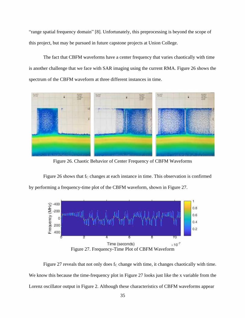
The fact that CBFM waveforms have a center frequency that varies chaotically with time

is another challenge that we face with SAR imaging using the current RMA. Figure 26 shows the

spectrum of the CBFM waveform at three different instances in time.

Figure 26. Chaotic Behavior of Center Frequency of CBFM Waveforms

Figure 26 shows that fC changes at each instance in time. This observation is confirmed

by performing a frequency-time plot of the CBFM waveform, shown in Figure 27.

Figure 27. Frequency-Time Plot of CBFM Waveform

Figure 27 reveals that not only does fC change with time, it changes chaotically with time.

We know this because the time-frequency plot in Figure 27 looks just like the x variable from the

Lorenz oscillator output in Figure 2. Although these characteristics of CBFM waveforms appear

36

detrimental to our current SAR imaging capabilities, since the RMA requires a constant fC

parameter, they reveal the anti-jamming quality of our CBFM radar. A jammer works by

blocking a certain range of frequencies, but if an agile frequency and pseudo-random waveform

is transmitted, it will be difficult to block.

Ranging

Due to difficulties we faced in trying to perform SAR imaging using CBFM waveforms,

it was decided to take a step back and explore using CBFM waveforms for ranging. Ranging is

much simpler than SAR imaging and utilizes the Range-Time Intensity Algorithm (RTIA). We

used the circuit-generated LFM and CBFM waveforms in our first ranging experiments, which

gave us the opportunity to compare LFM and CBFM results before we introduced MATLAB

generated signals. These tests serve as the control experiments throughout the rest of our testing.

The results of these tests are shown in Figure 28.

Figure 28. Circuit-Generated RTI Plots

In both experiments above, a team member stood in front of the radar and walked about

35-40m away, taking about 20 seconds. The team member then turned around and walked

directly back to the radar, taking about another 20 seconds. One can clearly see this movement in

37

the RTI plot on the left (Figure 28a) which used LFM. In contrast, the plot on the right, which

uses CBFM (Figure 28b), displays no information and appears as noise.

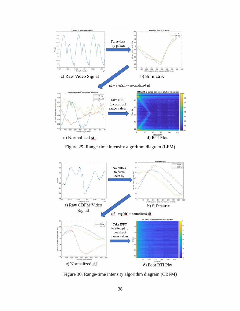
Troubleshooting Issues with CBFM for Ranging

To understand what is going wrong with our CBFM ranging experiments we must

discuss the RTIA in greater depth and uncover how, like the RMA used for SAR imaging, the

RTIA also inherently assumes the use of LFM waveforms. The RTIA starts with raw video data,

stored in the form of signal intensity vs. time. Using the sync pulses, the RTIA then parses the

data into a matrix called the “sif,” consisting of rows of signal intensity data for each 20ms pulse

of the linear ramp signal. The average of the sif is calculated and then subtracted from each row,

yielding the final “normalized” sif matrix. The RTIA then conducts the inverse Fast Fourier

Transform (IFFT) on the sif matrix. The IFFT allows the algorithm to reconstruct range values

for each one of these pulses, which are later combined to create the RTI plot. The problem lies in

that the IFFT is based on a known frequency vector that corresponds to the linear ramp signal, as

was seen in Figure 10. The algorithm “expects” the frequency to be a certain value, “x,” at each

point in the pulse based on this linear relationship. There does not appear to be a way to modify

the IFFT to incorporate a different frequency relationship based on chaotic signals like those

seen in Figure 16. The diagrams in Figure 29 and Figure 30 visualize the RTIA process using

LFM and CBFM waveforms.

38

Figure 29. Range-time intensity algorithm diagram (LFM)

Figure 30. Range-time intensity algorithm diagram (CBFM)

39

In summary, chaos signals do not work with the RTIA for two major reasons. First, raw

data collected with CBFM will not have regular pulses like Figure 29a). Second, between Figure

30c) and Figure 30d), chaotic signals do not exhibit the linear relationship that the IFFT

“expects” when constructing range values for the RTI plot.

MATLAB-Generated Signal Results

Fortunately, the MATLAB-generated quasi-LFM signals that were discussed in the

background section can help alleviate the problems we experienced with the use of circuit-

generated chaos for ranging. Figure 31 below is the same as Figure 28a) except that a MATLAB-

generated LFM signal is used instead of a circuit-generated LFM signal. This is our base case

experiment.

Figure 31. MATLAB-generated LFM RTI plot

The following series of figures are the results of the sensitivity experiment that was

proposed in the Design section of this report. Each plot uses MATLAB-generated quasi-LFM

signals, but the compression factor (C) is increased slightly each time to see the effect that

oscillation rate has on the RTI plot quality. Figure 11 and Figure 13 show the five waveforms

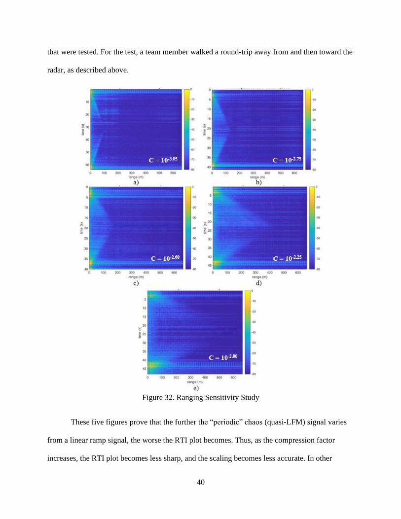
40

that were tested. For the test, a team member walked a round-trip away from and then toward the

radar, as described above.

Figure 32. Ranging Sensitivity Study

These five figures prove that the further the “periodic” chaos (quasi-LFM) signal varies

from a linear ramp signal, the worse the RTI plot becomes. Thus, as the compression factor

increases, the RTI plot becomes less sharp, and the scaling becomes less accurate. In other

41

words, the larger the C value, the more oscillations there are in the quasi-LFM signal, and the

less accurate our plot is. Therefore, a value between C = 10-3.05 and C = 10-2.75 is ideal for quasi-

LFM ranging.

A similar sensitivity study was performed for SAR imaging using MATLAB-generated

quasi-LFM signals. The “Steinmetz Car” target was used again for this sensitivity study. The

figures below show the results of those experiments.

Figure 33. SAR Sensitivity Study

These results are consistent with the trend we observed in our ranging experiments. As

the compression factor increases, the worse the SAR image quality gets. However, even the

smallest variation away from pure LFM waveform produced very poor results, seen in Figure

42

33b) with C = 10-3.05. Figure 33a, the base case LFM image, shows distinct hotspots that indicate

objects in the target scene, whereas Figure 33b) used the smallest compression value and objects

cannot be easily distinguished in the target scene. Our results show that the RMA is extremely

sensitive to any variations away from linear ramp signals and that SAR imaging with the current

RMA can only be performed using pure LFM waveforms.

Future Work

The most important area of work that needs to be addressed in the future is the signal

preprocessing into the range spatial frequency domain that is required when using non-linear FM

waveforms. Although we believe such preprocessing to be the key that will make SAR imaging

function with CBFM waveforms, we did not have sufficient time to explore this approach.

In addition, the creation of a simple, indoor target environment would also be highly

beneficial for any group working on this project in the future. We spent a significant amount of

time transporting our radar system between ISEC and the target scene by the Steinmetz car. The

target scene was also too complex, as there were multiple buildings, cars, corners, and elevations

that made multiple objects in the target scene hard to differentiate from each other. A single

object in an open indoor room would be a superior choice for a target.

There are also many ways that the radar itself can be approved. First, a periodic chaos

circuit could be created using circuitry and an embedded microcontroller. This would eliminate

the need for a second laptop that is currently being used to generate the periodic chaos in

MATLAB. Second, the compression factor value could be optimized to produce the best quasi-

LFM results. We determined the ideal range to be somewhere between C = 10-3.05 and C = 10-2.75,

but we did not test any values in between. Lastly, the physical radar apparatus has significant

43

room for improvement. Since the radar’s beam pattern is conical, we receive significant

reflections from the ground within 10-15m directly in front of the radar’s antenna, seen in Figure

23 and Figure 33. This could be fixed by mounting the radar higher off the ground, or by tilting

the radar slightly upwards, so that those reflections are not as severe. We also did not have the

chance to tune the radar antenna to minimize its reflection coefficient, which would further

optimize the imaging quality.

Conclusion

In conclusion, throughout the course of this project, problem simplification was critical to

making progress. Even though taking a step “backwards” to ranging from SAR imaging felt like

we were headed in the wrong direction, this decision helped us make much more progress

towards the end goal of this project than if we had kept trying to work on SAR. By focusing on

ranging, we acquired a much deeper understanding of the inherent characteristics of aperiodic

chaos signals that make it difficult to use with current radar imaging algorithms. It was in taking

this step back that we realized that we could utilize the quasi-LFM signals discussed in [7] by

creating “periodic” chaos signals in MATLAB. These periodic, slowly oscillating chaos signals

yielded suitable RTI plots for ranging while retaining the benefit of the anti-jamming properties

of chaos-based radar. Finally, we found that both the RTIA and the RMA will need major

modifications to make use of chaos-based waveforms. This project was not easy by any means,

but my partner Rong Chen and I have learned a great deal about the subjects of signal

processing, RF design, MATLAB software, chaos theory and hard work. We will bring these

skills into our graduate studies and beyond. To the best of our knowledge, we tried to construct

one of the first chaos-based frequency modulated radar systems in the world.

44

References

[1] M. I. Skolnik, "History of Radar," Encyclopedia Britannica, 26 July 1999. [Online].

Available: https://www.britannica.com/technology/radar/History-of-radar. [Accessed 24

November 2020].

[2] M. A. Richards, J. A. Scheer and W. A. Holm, Principles of Modern Radar, Raleigh, NC:

SciTech Publishing, 2010.

[3] G. L. Charvat, "Build a Small Radar System Capable of Sensing Range, Doppler, and

Synthetic Aperture Radar Imaging," MIT OpenCourseWare, [Online]. Available:

https://ocw.mit.edu/resources/res-ll-003-build-a-small-radar-system-capable-of-sensing-

range-doppler-and-synthetic-aperture-radar-imaging-january-iap-2011/#. [Accessed 24

November 2020].

[4] A. N. Beal, S. D. Cohen and T. M. Syed, "Generating and Detecting Solvable Chaos at

Radio Frequencies with Consideration to Multi-User Ranging," MDPI: Sensors, vol. 20,

no. 774, pp. 1-24, 2020.

[5] G. L. Charvat, A. J. Fenn and B. T. Perry, "The MIT IAP radar course: Build a small radar

system capable of sensing range, Doppler, and synthetic aperture (SAR) imaging," in IEEE

Radar Conference, Atlanta, GA, 2012.

[6] P. Horowitz, "Build a Lorenz Attractor," seti.Harvard.edu, [Online]. Available:

http://seti.harvard.edu/unusual_stuff/misc/lorenz.htm. [Accessed 24 November 2020].

[7] B. Flores, C. Pappu and B. Verdin, "Generation of FM signals with quasi-chirp behavior

using three-dimensional chaotic flows," in Proceedings of SPIE, San Diego, CA, 2011.

[8] W. Carrara, R. Goodman and R. Majewski, Spotlight Synthetic Aperture Radar Signal

Processing Algorithms, Boston, MA: Artech House, 1995.

[9] K. Meza and D. Coker, "Coffee Can Radar System," Dept. Electrical Engineering, Union

College, 26 March 2020. [Online]. Available: https://cpb-us-

w2.wpmucdn.com/muse.union.edu/dist/0/594/files/2020/03/Capstone-

Thesis_Meza_Rev2_March_26th_2020.pdf. [Accessed 17 March 2021].

[10] "IEEE Code of Ethics," IEEE.org, [Online]. Available:

https://www.ieee.org/about/corporate/governance/p7-8.html. [Accessed 19 November

2020].

[11] G. L. Charvat, A Low-Power Radar Imaging System, 2nd Edition, East Lansing: Michigan

State University, 2007.

45

[12] "686-2017 - IEEE Standard for Radar Definitions," Standards.IEEE.org, [Online].

Available: https://standards.ieee.org/standard/686-2017.html. [Accessed 6 June 2020].

[13] "1910.97 - Nonionizing Radiation," OSHA.gov, [Online]. Available:

https://www.osha.gov/laws-regs/regulations/standardnumber/1910/1910.97. [Accessed 6

June 2020].

[14] "521-2019 - IEEE Standard Letter Designations for Radar-Frequency Bands,"

Standards.IEEE.org, [Online]. Available: https://standards.ieee.org/standard/521-

2019.html. [Accessed 6 June 2020].

Appendices

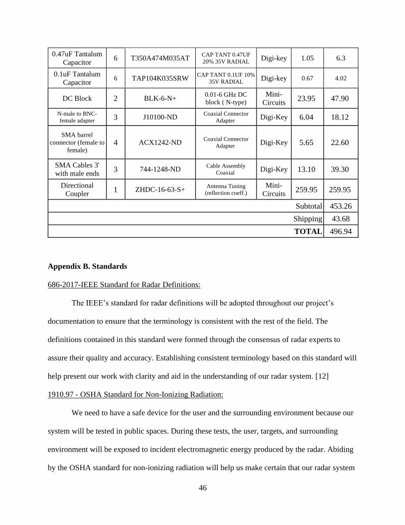
Appendix A. Complete Parts List and Funding Requested

Total Funding that was requested was $496.94.

Object Qty. Part # Description Supplier Unit

Cost ($)

Subtotal

($)

Analog

multiplier 3 AD633JN

Analog Multiplier 4-

Quadrant 8-PDIP Jameco 12.49 37.47

OPAMP 6 LM741CN/NOPB IC OPAMP GP 1

CIRCUIT 8DIP Digi-key 0.87 5.22

100k Resistor 4 MFP-25BRD52-100K RES 100K OHM 1/4W

0.1% AXIAL Digi-key 0.61 2.44

35.7k Resistor 3 MFR-25FBF52-35K7 RES 35.7K OHM 1/4W

1% AXIAL Digi-key 0.10 0.30

10k Resistor 4 MFP-25BRD52-10K RES 10K OHM 1/4W

0.1% AXIAL Digi-key 0.61 2.44

374k Resistor 3 MFR-25FBF52-374K RES 374K OHM 1/4W

1% AXIAL Digi-key 0.10 0.30

1M Resistor 2 YR1B1M0CC RES 1.00M OHM

1/4W 0.1% AXIAL Digi-key 0.57 1.14

0.47uF

Electrolytic

Capacitor 5 UKL2AR47KDD

CAP ALUM 0.47UF

10% 100V RADIAL Digi-key 0.35 1.75

0.1uF Electrolytic

Capacitor 5 UKL2A0R1KDD

CAP ALUM 0.1UF

10% 100V RADIAL Digi-key 0.39 1.95

2000pF Tantalum

Capacitor 10 S202M29Z5UN63L6R

CAP CER 2000PF 1KV

Z5U RADIAL Digi-key 0.206 2.06

46

0.47uF Tantalum

Capacitor 6 T350A474M035AT

CAP TANT 0.47UF

20% 35V RADIAL Digi-key 1.05 6.3

0.1uF Tantalum

Capacitor 6 TAP104K035SRW

CAP TANT 0.1UF 10%

35V RADIAL Digi-key 0.67 4.02

DC Block 2 BLK-6-N+ 0.01-6 GHz DC

block ( N-type) Mini-

Circuits 23.95 47.90

N-male to BNC-

female adapter 3 J10100-ND Coaxial Connector

Adapter Digi-Key 6.04 18.12

SMA barrel

connector (female to

female) 4 ACX1242-ND

Coaxial Connector

Adapter Digi-Key 5.65 22.60

SMA Cables 3'

with male ends 3 744-1248-ND

Cable Assembly

Coaxial Digi-Key 13.10 39.30

Directional

Coupler 1 ZHDC-16-63-S+

Antenna Tuning

(reflection coeff.) Mini-

Circuits 259.95 259.95

Subtotal 453.26

Shipping 43.68

TOTAL 496.94

Appendix B. Standards

686-2017-IEEE Standard for Radar Definitions:

The IEEE’s standard for radar definitions will be adopted throughout our project’s

documentation to ensure that the terminology is consistent with the rest of the field. The

definitions contained in this standard were formed through the consensus of radar experts to

assure their quality and accuracy. Establishing consistent terminology based on this standard will

help present our work with clarity and aid in the understanding of our radar system. [12]

1910.97 - OSHA Standard for Non-Ionizing Radiation:

We need to have a safe device for the user and the surrounding environment because our

system will be tested in public spaces. During these tests, the user, targets, and surrounding

environment will be exposed to incident electromagnetic energy produced by the radar. Abiding

by the OSHA standard for non-ionizing radiation will help us make certain that our radar system

47

is safe to use. This OSHA standard specifies 10mW/cm2 averaged over any 0.1-hour period as

the maximum limit for incident electromagnetic energy exposure. Given this power density limit,

we can determine the maximum power limit for our transmitted signals. [13]

521-2019 - IEEE Standard for Letter Designations for Radar-Frequency Bands:

This IEEE standard covers the letters in common usage for the frequency ranges that they

represent. We will refer to this standard in our documentation when naming the frequency band

used by our radar so that the labeling agrees with experts in this field. Like the IEEE terminology

standard, this will help us prevent any confusion or inconsistency in our project’s documentation.

This will be important in the future when we aren’t present to explain which frequency band we

used and how we labeled it. This standard will also help us avoid using the incorrect frequency

bands for our specific application. We do not want to cause interference in any other

communication systems. [14]