changes in dissolved iron deposition to the oceans...

Biogeosciences, 12, 3973–3992, 2015

www.biogeosciences.net/12/3973/2015/

doi:10.5194/bg-12-3973-2015

© Author(s) 2015. CC Attribution 3.0 License.

Changes in dissolved iron deposition to the oceans driven by human

activity: a 3-D global modelling study

S. Myriokefalitakis1, N. Daskalakis1,2, N. Mihalopoulos1,3, A. R. Baker4, A. Nenes2,5,6, and M. Kanakidou1

1Environmental Chemical Processes Laboratory, Department of Chemistry, University of Crete,

P.O. Box 2208, 70013 Heraklion, Greece2Institute of Chemical Engineering Sciences (ICE-HT), FORTH, Patras, Greece3Institute for Environmental Research and Sustainable Development, National Observatory of Athens,

Athens, Greece4School of Environmental Sciences, University of East Anglia, Norwich, NR4 7TJ, UK5School of Earth and Atmospheric Sciences, Georgia Institute of Technology, 311 Ferst Drive,

Atlanta, GA 30332-0100, USA6School of Chemical and Biomolecular Engineering, Georgia Institute of Technology, 311 Ferst Drive,

Atlanta, GA 30332-0100, USA

Correspondence to: S. Myriokefalitakis ([email protected]) and M. Kanakidou ([email protected])

Received: 31 December 2014 – Published in Biogeosciences Discuss.: 02 March 2015

Revised: 31 May 2015 – Accepted: 09 June 2015 – Published: 02 July 2015

Abstract. The global atmospheric iron (Fe) cycle is pa-

rameterized in the global 3-D chemical transport model

TM4-ECPL to simulate the proton- and the organic ligand-

promoted mineral-Fe dissolution as well as the aqueous-

phase photochemical reactions between the oxidative states

of Fe (III/II). Primary emissions of total (TFe) and dissolved

(DFe) Fe associated with dust and combustion processes are

also taken into account, with TFe mineral emissions cal-

culated to amount to ∼ 35 Tg-Fe yr−1 and TFe emissions

from combustion sources of ∼ 2 Tg-Fe yr−1. The model rea-

sonably simulates the available Fe observations, supporting

the reliability of the results of this study. Proton- and or-

ganic ligand-promoted Fe dissolution in present-day TM4-

ECPL simulations is calculated to be ∼ 0.175 Tg-Fe yr−1,

approximately half of the calculated total primary DFe emis-

sions from mineral and combustion sources in the model

(∼ 0.322 Tg-Fe yr−1). The atmospheric burden of DFe is

calculated to be ∼ 0.024 Tg-Fe. DFe deposition presents

strong spatial and temporal variability with an annual flux

of ∼ 0.496 Tg-Fe yr−1, from which about 40 % (∼ 0.191 Tg-

Fe yr−1) is deposited over the ocean. The impact of air qual-

ity on Fe deposition is studied by performing sensitivity sim-

ulations using preindustrial (year 1850), present (year 2008)

and future (year 2100) emission scenarios. These simulations

indicate that about a 3 times increase in Fe dissolution may

have occurred in the past 150 years due to increasing anthro-

pogenic emissions and thus atmospheric acidity. Air-quality

regulations of anthropogenic emissions are projected to de-

crease atmospheric acidity in the near future, reducing to

about half the dust-Fe dissolution relative to the present day.

The organic ligand contribution to Fe dissolution shows an

inverse relationship to the atmospheric acidity, thus its im-

portance has decreased since the preindustrial period but is

projected to increase in the future. The calculated changes

also show that the atmospheric DFe supply to the globe has

more than doubled since the preindustrial period due to 8-

fold increases in the primary non-dust emissions and about

a 3-fold increase in the dust-Fe dissolution flux. However,

in the future the DFe deposition flux is expected to decrease

(by about 25 %) due to reductions in the primary non-dust

emissions (about 15 %) and in the dust-Fe dissolution flux

(about 55 %). The present level of atmospheric deposition of

DFe over the global ocean is calculated to be about 3 times

higher than for 1850 emissions, and about a 30 % decrease

is projected for 2100 emissions. These changes are expected

to impact most on the high-nutrient–low-chlorophyll oceanic

regions.

Published by Copernicus Publications on behalf of the European Geosciences Union.

3974 S. Myriokefalitakis et al.: Changes in dissolved iron deposition to the oceans driven

1 Introduction

Atmospheric deposition of trace constituents, both of natural

and anthropogenic origin, can act as a nutrient source into

the open ocean and therefore can affect marine ecosystem

functioning and subsequently the exchanges of CO2 between

the atmosphere and the global ocean (Duce et al., 2008).

In surface waters, the phytoplankton photosynthetic activity

uses CO2 and nutrients to produce biomass and is respon-

sible for nearly half of annual CO2 exchange with the deep

ocean that contains∼ 85 % of Earth’s mobile carbon (Shao et

al., 2011). This is the so-called “biological pump”, where the

deeper the carbon sinks, the longer it will be removed from

the atmosphere (Falkowski et al., 2000). The net result of the

biological pump is a continual atmospheric carbon transfer

to the deep ocean. Aeolian dust deposition, calculated to be

∼ 1257 Tg yr−1 (median of 15 global models by Huneeus et

al., 2011), contains∼ 3.5 % iron (Fe) on average, and it is the

most significant external supply of Fe (as a micronutrient)

in surface waters (Taylor and McLennan, 1985; Mahowald

et al., 2005, 2009). Fe scarcity limits phytoplankton produc-

tivity in high-nutrient–low-chlorophyll (HNLC) regions (i.e.

the Southern Ocean, the eastern equatorial and the subarc-

tic Pacific; Boyd et al., 2005) and thus primary productivity

in large portions of the global ocean, significantly affecting

the biological carbon export on a global scale (Maher et al.,

2010). The correlation between Fe supply and atmospheric

CO2-trapping to the ocean forms the so-called “Iron Hypoth-

esis” (Martin and Fitzwater, 1988) that initiated significant

scientific debate on the potential use of Fe to fertilize the

global ocean (i.e. geoengineering) and consequently increase

CO2 storage in the ocean (e.g. Moore and Doney, 2007).

The bioavailable form of Fe that is acquired by phyto-

plankton is associated with the soluble fraction of Fe, which

is measured experimentally as the fraction filterable through

0.2–0.45 µm filters (Kraemer, 2004). Aerosols are emitted or

formed, transported and deliquesce in the atmosphere (Raes

et al., 2000). Processes that occur in the water associated with

aerosols can change aerosol properties. There is experimental

evidence that atmospheric acidity is increasing dust solubil-

ity (e.g. Nenes et al., 2011) and that present-day atmospheric

acidity is mainly driven by air pollution (Seinfeld and Pan-

dis, 1998 and references therein). Although the fraction of

soluble Fe in soil is low (∼ 0.1 %; Mahowald et al., 2009

and references therein); atmospheric chemical processes are

responsible for Fe conversion to more soluble forms (Ma-

howald et al., 2009), and thus bioavailable form for the ocean

biota. Dust coating by acid-soluble materials (e.g. nitrates,

sulfates) also alters the global pattern of Fe deposition (Fan

et al., 2004).

Significant scientific effort has been made to understand

the impact of anthropogenically driven atmospheric acid-

ity on dust and parameterize it in global models. To study

the aforementioned changes in dust-Fe solubility driven by

human activities, atmospheric models need to account for

both (i) the composition of the Fe source and (ii) the atmo-

spheric aging of dust. However, the atmospheric chemical

aging of dust with respect to dissolved/bioavailable Fe (here-

after DFe) production is parameterized in chemistry transport

models (CTMs) in different ways. In the modelling study of

Meskhidze et al. (2005), hematite (Fe2O3) was considered as

the only Fe-containing mineral in dust (5 % mass fraction of

hematite in dust) and the proton-promoted Fe dissolution was

described using the empirical parameterization developed by

Lasaga et al. (1994). That study simulated the production of

DFe in the ferric oxidation state (Fe(III)) but did not account

for any photochemical cycling between Fe(III) and Fe(II).

Luo et al. (2008), using the same approximation, consid-

ered the formation of DFe in the ferrous form (Fe(II)) during

Fe-containing mineral dissolution. In support of the proton-

promoted Fe dissolution hypothesis, a positive correlation

of Fe solubility (hereafter SFe; SFe= 100×DFe /TFe) and

sulfur emissions has been observed for acidic atmospheric

samples collected at urban sites (Oakes et al., 2012). The

simulations by Solmon et al. (2009) suggest that the doubling

of sulfur emissions can increase the proton-promoted disso-

lution and deposition of dissolved Fe to the remote Pacific

Ocean by ∼ 13 %.

Fe dissolution from minerals under acidic conditions oc-

curs on different timescales; from hours to weeks depending

on the size and the type of the Fe-containing mineral (Shi et

al., 2011a). However, the buffering capacity of minerals, like

CaCO3 and MgCO3, which reside in coarse dust particles,

may regulate mineral-Fe proton-promoted dissolution, con-

tributing, among others, together with combustion emissions

of DFe on fine particles and atmospheric transport, to an ob-

served inverse relationship between SFe and particle size (Ito

and Feng, 2010). A recent CTM study (Ito and Xu, 2014)

simulated the present-day SFe over the Northern Hemisphere

oceans reasonably well, and calculated the proton-promoted

dissolution of Fe in the year 2100, considering three pools

of Fe-containing minerals depending on their timescale of

potential for Fe dissolution, based on the findings of Shi et

al. (2011b; 2012).

Laboratory studies have also shown the occurrence of pho-

toinduced reductive Fe dissolution under rather acidic con-

ditions (e.g. pH< 4), suggesting a steady-state Fe(II) pro-

duction during exposure of dust to solar radiation and thus

increased daytime dissolution rate of hematite compared to

standard kinetics (Zhu et al., 1993; Jickells and Spokes, 2001

and references therein). However, the dust-Fe dissolution

through photoreduction only has a limited impact (< 1 %)

on the DFe concentration (Zhu et al., 1993). Moreover, ex-

perimental data also support that both inorganic (e.g. sulfu-

ric and nitric acid) and organic (e.g. oxalic and acetic acid)

acids can increase Fe dissolution (Paris et al., 2011; Paris

and Desboeufs, 2013). Laboratory investigations (Chen and

Grassian, 2013) also indicate that the relative capacity of ox-

alic acid in acidic solution (pH= 2) is by far the most impor-

tant for Fe dissolution in dust and combustion aerosols com-

Biogeosciences, 12, 3973–3992, 2015 www.biogeosciences.net/12/3973/2015/

S. Myriokefalitakis et al.: Changes in dissolved iron deposition to the oceans driven 3975

pared to sulfuric acid due, to the formation of mononuclear

bidentate ligand with surface Fe, in contrast to the weaker

complexes formed from HSO−4 and SO2−4 .

Oxalic acid/oxalate (hereafter OXL) is globally the most

abundant dicarboxylic acid, formed via chemical oxidation

of both biogenic and anthropogenic gas-phase precursors

in the aqueous phase of aerosols and cloud droplets (e.g.

Carlton et al., 2007; Lim et al., 2010). Johnson and Me-

skindze (2013) calculated that the ligand (OXL) -promoted

Fe dissolution and Fe(II) /Fe(III) redox cycling of Fe con-

tent of mineral dust in both aerosol and cloud water increased

total annual calculated DFe deposition to global oceanic

regions by ∼75 %, compared to only proton-promoted Fe

dissolution simulations. However, the aforementioned study

used sulfate aerosol as a proxy for the occurrence of OXL

and took three Fe-containing dust minerals (i.e. goethite,

hematite and illite) into account, as studied by Paris et

al. (2011). A recent modelling study by Ito (2015), published

after the submission of the present work, focusing on the at-

mospheric processing of Fe-containing combustion aerosols

by photochemical reactions with inorganic and organic acids,

indicates that ligand (OXL)-promoted Fe dissolution more

than doubles the calculated DFe deposition from combustion

sources over certain regions of the global ocean.

Besides proton- and ligand-promoted mineral-Fe disso-

lution, primary emissions of Fe, especially from combus-

tion processes, can lead to an increase in the SFe fraction.

Mineral-Fe represents∼ 95 % of the global atmospheric TFe

source, with combustion Fe sources responsible for the re-

maining ∼ 5 % (Luo et al., 2008; Mahowald et al., 2009).

Luo et al. (2008) accounted for both soluble and insolu-

ble forms of Fe emissions from biomass burning and an-

thropogenic combustion processes in relation to black car-

bon (BC) emissions and they estimated (based on observed

Fe /BC ratios) that ∼ 1.7 Tg-Fe yr−1 are emitted to the at-

mosphere via combustion processes. Mahowald et al. (2009)

also indicate that humans may significantly impact DFe de-

position over oceans by increasing both the acidity of atmo-

spheric aerosol, as well as the DFe emissions from combus-

tion processes. Model projections for the year 2100 suggest

that fossil fuel combustion aerosols from shipping could con-

tribute up to∼ 60 % of DFe deposition to remote oceans (Ito,

2013).

In the present study, the 3-D chemical transport global

model TM4-ECPL, that explicitly calculates aqueous-phase

chemistry of OXL and the photochemical cycle of the at-

mospheric Fe cycle, is used to simulate Fe deposition over

land and oceans, accounting for five Fe-containing dust min-

erals and for anthropogenic emissions of Fe. Following the

scheme of Ito and Xu (2014), dissolution of Fe (Sect. 2)

from three pools of minerals (Shi et al., 2012) is consid-

ered here to occur by proton-promoted dissolution on three

characteristic timescales and by ligand (OXL)-promoted dis-

solution (as demonstrated by Paris et al., 2011 and param-

eterized by Johnson and Meskindze, 2013). The calculated

TFe and DFe global atmospheric budgets and distributions

are presented and compared to observations in Sect. 3. The

importance of air pollutants for DFe atmospheric concentra-

tions and deposition is investigated in Sect. 4, based on sim-

ulations using past and future anthropogenic and biomass-

burning emissions scenarios. The significant contribution of

anthropogenic sources to the dissolution of Fe-containing

minerals, their impact on DFe deposition over oceans and

the implications of the findings for the biogeochemistry of

marine ecosystems are summarized in Sect. 5.

2 Model description

The TM4-ECPL global chemistry transport model

(Myriokefalitakis et al., 2011; Daskalakis et al., 2015

and references therein) is able to simulate oxidant

(O3 /NOx /HOx /CH4 /CO) chemistry, accounting

for non-methane volatile organic compounds (NMVOCs,

including isoprene, terpenes and aromatics), as well as all

major aerosol components, including secondary aerosols like

sulfate (SO2−4 ), nitrate (NO−3 ) and ammonium (NH+4 ), using

the ISORROPIA II thermodynamic model (Fountoukis and

Nenes, 2007) and secondary organic aerosols (SOA) (Tsi-

garidis and Kanakidou, 2003, 2007). Compared to its parent

TM4 model (van Noije et al., 2004), the current version has

a comprehensive description of chemistry (Myriokefalitakis

et al., 2008) and organic aerosols (Myriokefalitakis et al.,

2010). It also accounts for multiphase chemistry in clouds

and aerosol water that produces OXL and affects SOA

formation (Myriokefalitakis et al., 2011).

For the present study, the TM4-ECPL model is driven

by ECMWF (European Center for Medium-Range Weather

Forecasts) Interim re-analysis project (ERA-Interim) mete-

orology (Dee et al., 2011). Advection of the tracers in the

model is parameterized using the slopes scheme (Russell

and Lerner, 1981 and references therein). Convective trans-

port is parameterized based on Tiedke (1989) and the Olivie

et al. (2004) scheme. Vertical diffusion is parameterized as

described in Louis (1979). For wet deposition, both large-

scale and convective precipitation are considered. In-cloud

and below-cloud scavenging is parameterized in TM4-ECPL

as described in detail by Jeuken et al. (2001). In-cloud scav-

enging of water-soluble gases is calculated, accounting for

the solubility of the gases (effective Henry law coefficients;

Tsigaridis et al., 2006; Myriokefalitakis et al., 2011 and ref-

erences therein). Dry deposition for all fine aerosol compo-

nents is parameterized similarly to that of nss-SO2−4 , which

follows Tsigaridis et al. (2006). Gravitational settling (Sein-

feld and Pandis, 1998) is applied to all aerosol components

and is an important dry deposition process for coarse parti-

cles like dust and sea salt. The current model configuration

has a horizontal resolution of 3◦ in longitude, by 2◦ in lati-

tude and 34 hybrid layers in the vertical, from the surface up

www.biogeosciences.net/12/3973/2015/ Biogeosciences, 12, 3973–3992, 2015


Table 1. Emissions of dust (in Tg yr−1), Fe contained in dust-minerals (illite, kaolinite, smectite, hematite and feldspars; in Tg-Fe yr−1) and

TFe and DFe (in Tg-Fe yr−1) used in TM4-ECPL for (a) present (year 2008), (b) past (year 1850) and (c) future (year 2100) simulations.

Species Year Biomass burning Anthropogenic combustion Ships’ oil combustion Soils

Dust 2008 1091

Fe (illite) 2008 8.473

Fe (kaolinite) 2008 0.871

Fe (smectite) 2008 17.154

Fe (hematite∗) 2008 5.663

Fe (feldspars) 2008 2.761

TFe 1850 0.120 0.147 9.83E-05 35.048

2008 1.200 0.768 0.015

2100 1.456 0.158 0.002

DFe 1850 0.013 0.011 7.99E-05 0.125

2008 0.127 0.058 0.012

2100 0.155 0.012 0.001

∗ Hematite is used here as a surrogate for hematite and goethite.

to 0.1 hPa. All simulations have been performed with meteo-

rology of the year 2008 and a model time step of 30 min.

2.1 Emissions

TM4-ECPL uses the anthropogenic and biomass-burning

emissions (NMVOC, nitrogen oxides (NOx), CO, SO2,

NH3, particulate organic carbon (OC) and black car-

bon (BC)) from the ACCMIP database (Lamarque et

al., 2013; http://eccad.sedoo.fr/eccad_extract_interface/JSF/

page_meta.jsf). Biogenic emissions (isoprene, terpenes, ac-

etaldehyde, acetone, ethane, ethene, propane, propene,

formaldehyde, CO, methyl ethyl ketone, toluene, methanol)

come from the MEGAN-MACC biogenic emissions in-

ventory for the year 2008 (Sindelarova et al., 2014). Soil

NOx and oceanic emissions (CO, ethane, ethene, propane,

propene) are taken from the POET (Granier et al., 2005) in-

ventory database (http://eccad.sedoo.fr). Oceanic emissions

of primary organic aerosol, isoprene, terpenes and sea-salt

particles are calculated online, driven by meteorology fol-

lowing Myriokefalitakis et al. (2010). Dust emissions are ob-

tained from the daily AEROCOM inventories (Aerosol Com-

parison between Observations and Models; Dentener et al.,

2006) updated to the year 2008 (E. Vignati, personal com-

munication, 2011). The anthropogenic and biomass-burning

emissions (NMVOC, NOx , CO, SO2, NH3, OC and BC)

from the ACCMIP database (Lamarque et al., 2013) for the

years: 1850 (hereafter PAST), 2008 (hereafter PRESENT)

and for the year 2100 based on the RCP6 emission scenario

(hereafter FUTURE), have been used for the different sim-

ulations as further explained. A summary of the emissions

considered in the model is given in Table S1 in the Supple-

ment.

2.2 Dust iron-containing mineral emissions

Various Fe-containing clay minerals (illite, kaolinite and

smectite), oxides (hematite and goethite) and feldspars can

be found in mineral dust (Nickovic et al., 2013). In the

present study, the global soil mineralogy data set developed

by Nickovic et al. (2012) at a 30′′ resolution (∼ 1 km) has

been initially re-gridded to 1◦× 1◦ global resolution and ap-

plied to the 1◦× 1◦ daily dust emissions taken into account

by TM4-ECPL. The percentage content in Fe of the differ-

ent Fe-containing minerals of dust that are considered in

the model has been taken from Nickovic et al. (2013) (il-

lite 4.8, kaolinite 0.7, smectite 16.4, goethite and hematite

66 and feldspar 2.5 %). Given this, the annual global mean

Fe content of emitted dust particles in TM4-ECPL is calcu-

lated to be ∼ 3.2 %. Despite differences in the chemical re-

activity and iron content of goethite and hematite (e.g. see

http://webmineral.com), these minerals are considered here

as one surrogate species, the hematite, used as proxy for Fe

oxides as suggested by Nickovic et al. (2012).

Based on the aforementioned soil mineralogy database

(FMIN_DUST), the daily dust emissions (DustEmi) in the model

and the Fe content of the minerals (FFeMIN ), TM4-ECPL cal-

culates the TFe emissions (FeEmi) from soils as

FeEmi = DustEmi×FMin_Dust×FFe_Min. (1)

Thus, the model accounts for the following annual Fe emis-

sions from soils: ∼ 8.473 from illite, ∼ 0.871 from kaoli-

nite, ∼ 17.154 from smectite, ∼ 5.663 from hematite and

goethite and∼ 2.761 Tg-Fe yr−1 from feldspars (Table 1), to-

tal ∼ 35.048 Tg-Fe yr−1. The DFe emissions in the form of

impurities in soils are prescribed in the initial dust sources as

4.3 % on kaolinite and 3 % on feldspars, as suggested by Ito

and Xu (2014) and account for ∼ 0.125 Tg-Fe yr−1. A sum-

mary of dust and Fe-containing mineral emissions used in the

TM4-ECPL model is provided in Table 1. The annual mean


http://eccad.sedoo.fr/eccad_extract_interface/JSF/page_meta.jsf

http://eccad.sedoo.fr/eccad_extract_interface/JSF/page_meta.jsf

http://eccad.sedoo.fr

http://webmineral.com


spatial distributions of dust (Fig. S1a in Supplement) and

emissions of Fe contained in different minerals (Fig. S1b–f)

as calculated by the model are also shown in the supplement.

2.3 Anthropogenic and biomass-burning iron emissions

TFe emissions from combustion sources have been estimated

at 1.07 from biomass burning, 0.66 from coal combustion

(Luo et al., 2008) and∼ 0.016 Tg-Fe yr−1 from shipping (Ito

et al., 2013), all for the year 2001. For this work, global and

monthly mean scaling factors of TFe emissions to those of

BC (Fe /BC) for each of the above mentioned emission sec-

tors have been derived based on emission estimates provided

by Luo et al. (2008) and the BC sources from the ACCMIP

database for the year 2001. Furthermore, to calculate the DFe

in primary emissions (both in fine and coarse particles), the

DFe emission estimates by Ito (2013) of 0.127 from biomass

burning, 0.055 from coal combustion and 0.013 Tg-Fe yr−1

from shipping, have been used together with the TFe emis-

sions mentioned above for the year 2001 (Luo et al., 2008)

to derive mean solubility for each of these three emission

categories. These are ∼ 12 for biomass-burning Fe sources,

∼ 8 for coal combustion and ∼ 81 % for shipping. The de-

rived Fe /BC emission ratios and the mean Fe solubility per

source category are then applied to the BC emissions from

the ACCMIP database for the respective year, to compute

the past, present and future emissions of TFe and DFe. The

computed annual mean surface distributions of the TFe emit-

ted by anthropogenic emissions (including shipping), and

biomass burning used in the model (∼ 1.983 Tg-Fe yr−1 for

the year 2008) are depicted in Fig. S1g and h, respectively.

2.4 Mineral dissolution scheme

The model calculates the dissolution of Fe-containing miner-

als in the aerosol water and in the cloud droplets. TM4-ECPL

treats the Fe dissolution as a kinetic process that depends on

the concentrations of (i) H+ (proton-promoted Fe dissolu-

tion) and (ii) OXL (organic ligand-promoted Fe dissolution)

in the solution (Fig. 1).

2.4.1 Proton-promoted iron dissolution

The proton-promoted dissolution rate of minerals in aerosol

and cloud water is calculated by applying the empirical pa-

rameterization developed by Lasaga et al. (1994), taking the

saturation degree of the solution, the type of each mineral

(MIN) as well as the reactivity of Fe species and the ambient

temperature into account.

RFe = NFeMIN×KMIN(T )× a(H+)m× fMIN×AMIN, (2)

where RFe is the Fe-containing mineral dissolution rate

(moles of Fe per gram of MIN per s), NFeMIN is the number

of moles of Fe per mole of mineral, KMIN is the temperature

(T )-dependent dissolution reaction coefficient of the mineral

water

Dust-Fe

H+

OXL2-

Fe (III)

Fe(III)(OXL)n3-2n

Fe (II)

H2O2

OH NO3

NO2

HO2/O2-

hv HO2/O2

-

Fe(II)(OXL)n2-2n

Figure 1. Atmospheric processing of dust-Fe taken into account in

the model. Details on the chemical reactions are given in Table S2.

(mol m−2 s−1), α(H+) is the H+ activity in the solution, m

is the reaction order with respect to aqueous-phase protons,

AMIN is the specific surface area of the mineral (m2 g−1) and

fMIN accounts for the variation of the rate when deviating

from equilibrium. For the present study, the above formula-

tion is applied to each mineral concentration [MIN] (and not

to the bulk mass of dust aerosol), since the model describes

each mineral with a different tracer in the chemical scheme.

For the calculation of the deviation from equilibrium fMIN,

the Eq. (3) given by Ito and Xu (2014) is used:

fMIN = 1− (aFe3+ × a−nMIN

H+)/KeqMIN, (3)

where aFe3+ is the concentration of Fe(III) in the aque-

ous solution (mol L−1), nMIN is the stoichiometric ratio

(number of moles mobilized per mole of mineral) and

KeqMIN is the equilibrium constant for iron oxides forma-

tion (Fe(OH)3). Mineral dissolution rates and the related fac-

tors used in this study are listed in Table 2, separating be-

tween the DFe (attributed to the emissions), fast-released

iron (Fef), intermediate-released iron (FeI) and refractory

iron (FeR) (Shi et al., 2011b, 2012), as explicitly parame-

terized by Ito and Xu (2014). Aerosol water pH is calcu-

lated by the ISORROPIA II thermodynamic model which

solves the K+–Ca2+–Mg2+–NH+4 –Na+–SO2−4 –NO−3 –Cl−–

H2O aerosol system. Based on the composition of mineral

dust and sea-salt elements, ISORROPIA II in TM4-ECPL

takes the following mean percent mass content of particles

into account: Na+, 30.6 % on sea salt and 1.7 % on dust;

Ca2+, 1.2 % on sea salt; K+, 2.4 % on dust and 1.1 % on

sea salt and Mg2+, 1.5 % on dust (as magnesite; Ito and

Feng, 2010 – consistent with the observations of Formenti



Table 2. Constants used for proton-promoted iron dissolution rates and emissions calculations for different types of iron-containing minerals:

water-soluble/dissolved iron (DFe); fast-released iron (FeF); intermediate-released iron (FeI); slowly released iron (FeS); refractory iron

(FeR). The parentheses contain the percentage content of Fe type in each mineral.

Mineral Fe type KMIN (mol m−2 s−1) m AMIN (m2 g−1) Keq n

Illite FeF (2.7 %)a 1.17× 10−09 exp[9.2× 103(1/298-1/T)]b 1b,c 205b,e 41.7 2.75

FeS (97.3 %) 1.30× 10−11 exp[6.7× 103(1/298-1/T)]d 0.39d 90d

Smectite FeI (5 %)a 8.78× 10−10 exp[9.2× 103(1/298-1/T)]b 1b,c 125b,e 3.31 2.85

FeS (95 %) 8.10× 10−12 exp[6.7× 103(1/298-1/T)]d 0.3d 300 d

Hematite∗ FeR (100 %)b 1.80× 10−11 exp[9.2× 103(1/298-1/T)]b 0.5e 9b,a 0.44 2.85

Kaolinite DFe(4.3 %)b

FeR (95.7 %) 4.00× 10−11 exp[6.7× 103(1/298-1/T)]f 0.1f 20f 0.44b 2.85b

Feldspars DFe (3 %)b

FeR (97 %) 2.4× 10−10 exp[7.7× 103(1/298-1/T)]f 0.5f 1f 0.44b 2.85b

a Shi et al, 2011b; b Ito and Xu, 2014; c Lanzl et al., 2012; d Ito, 2012; e Bonneville et al., 2004; f Meskhidze et al., 2005 and references therein. ∗ Hematite

is used here as a surrogate for hematite and goethite.

et al., 2008) and 3.7 % on sea salt (http://geology.utah.gov/

online_html/pi/pi-39/pi39pg9.htm); Cl−, 55 % on sea salt;

and SO2−4 , 7.7 % on sea salt. The global soil mineralogy data

set (Nickovic et al., 2012) has been applied on dust emissions

to calculate the concentrations of Ca2+ on dust particles (i.e.

calcite (CaCO3) and gypsum (CaSO4)).

Aerosol pH and water are calculated here for each aerosol

mode (Fig. S2a for the fine mode and Fig. S2b for the

coarse mode). The pH values for each aerosol mode are

calculated by the thermodynamic equilibrium model ISOR-

ROPIA II assuming internal mixing of the aerosols (Foun-

toukis and Nenes, 2007). Briefly, for each mode (fine and

coarse) sulfate, nitrate, ammonium and sea-salt (i.e. K+;

Ca2+; Mg2+; Na+; SO2−4 ; Cl−) aerosols are assumed to be

internally mixed. Carbonates (CaCO3, MgCO3) and gypsum

(CaSO4) are considered to be present in the silt soil parti-

cles (Meskhidze et al., 2005), with their impact on the coarse

particulate H+ and H2O, to be calculated interactively by the

ISORROPIA II. The dissolved Ca2+ and Mg2+ is distributed

by the thermodynamic model among all possible solids.

In TM4-ECPL, in-cloud pH (Fig. S2c at ∼ 850 hPa and

Fig. S2d for zonal mean) is controlled by strong acids (sul-

fates, SO2−4 ; methanesulfonate, MS−; nitric acid, HNO3; ni-

trate ion, NO−3 ), bases (ammonium ion, NH+4 ), as well as by

the dissociations of hydrated CO2, SO2, NH3 and of oxalic

acid (Myriokefalitakis et al., 2011). Crustal and sea-salt el-

ements are not considered for pH calculations in the cloud

chemical scheme.

2.4.2 Organic ligand-promoted iron dissolution

Recent laboratory studies show a positive linear correlation

between iron solubility and organic ligands concentrations

(e.g. Paris and Desboeufs, 2011 and references therein). Two

mechanisms have been proposed concerning the mineral dis-

solution in the presence of organic ligands: (i) the non-

reductive (Stumm and Morgan, 1996) and (ii) the reductive

(Stumm and Sulzberger, 1992) ligand-promoted dissolution.

Experimental studies by Paris and Desboeufs (2013) indicate

that certain organic ligands (including OXL) enhance Fe dis-

solution from mineral dust. This ligand-promoted dissolution

was accompanied by increased concentrations of dissolved

Fe(II) and was probably related to the ability of organic lig-

ands to act as electron donors.

In the present study, we follow the recommendations of

Johnson and Meskhidze (2013) based on the experiments

by Paris et al. (2011) for OXL-promoted Fe dissolution of

hematite, goethite and illite in cloud droplets and rainwater.

Because the mineral database used for this study considers

the average iron oxides (the goethite and hematite content) as

a single iron oxide species (hematite), we take the fractional

OXL-promoted Fe dissolution rates for hematite (α-Fe2O3)

and goethite (α-FeO(OH)) into account proposed by Johnson

and Meskhidze (2013), as presented in Table 3. The average

values of relative proportions of Fe in the form of hematite

and goethite to total iron oxide are based on experimental

data for dust sources, compiled by Formenti et al. (2014),

with their abundance in total iron oxide at ∼ 36 and ∼ 64 %,

respectively.

DFe production during the organic ligand-promoted Fe

dissolution is considered here to be in the form of Fe(II)

-oxalato complexes in the aqueous phase (i.e. in the fer-

rous oxidation state) and it is only applied to water droplets

following the recommendations of the laboratory studies

by Paris et al. (2011) and Paris and Desboeufs (2013).

The aforementioned experiments have been performed with

OXL concentrations found typically in rainwater and cloud

droplets (0–8 µM), with a pH of 4.5 and dust concentrations

of about 15 mg L−1. Indeed, properties of the aqueous solu-

tion of clouds differ significantly to those of aerosols, with

higher pH values (e.g. > 4), lower aqueous-phase dust con-

centrations (< 50 mg L−1) and lower ionic strength (Shi et


http://geology.utah.gov/online_html/pi/pi-39/pi39pg9.htm

http://geology.utah.gov/online_html/pi/pi-39/pi39pg9.htm


Table 3. Constants used for ligand (oxalate)-promoted iron dissolution from illite and hematite.

Mineral Dissolution rates Amin Ref.

(mol Fe m−2 s−1) (m2 g−1)

Illite 3.00× 10−10 [OXL2−] + 6× 10−11 205 Paris et al. (2011);

Johnson and Meskhidze (2013)

Hematite∗ 0.36× (3.00× 10−12 [OXL2−]− 2× 10−12) 9 Paris et al. (2011);

+0.64× (1.00× 10−11 [OXL2−]+ 7× 10−13) Johnson and Meskhidze (2013)

∗ Hematite is used here as a surrogate for hematite and goethite.

al., 2012). On the other hand, the liquid aerosol content of

typical continental aerosols can vary between ∼10−12 and

10−11 cm3 cm−3 air, depending on the relative humidity, and

the aerosol pH can vary between 1 and 4 (McNeill et al.,

2012). Aqueous-phase OXL concentrations are significantly

related to the transfer of small gas-phase polar compounds

(e.g. glyoxal) to the liquid-phase (Carlton et al., 2007), a pro-

cess that depends proportionally on the volume of the aque-

ous medium and on the pH of the solution. On the other

hand, high acidic pH in the condense phase tends to favour

the production of oligomeric structures rather than OXL (e.g.

Lim et al., 2010, 2013). Thus, under such conditions of low

aqueous-phase OXL concentrations, the ligand-promoted Fe

dissolution may be suppressed significantly.

2.5 Aqueous-phase chemistry scheme

The global model simulates aqueous-phase chemistry in

aerosol water and cloud droplets as described in Myriokefali-

takis et al. (2011). To parameterize the Fe speciation through

the photochemical cycling of Fe(III) /Fe(II), the aqueous-

phase chemical scheme has been further developed to ac-

count for the mineral-Fe dissolution processes and the ferric-

and ferrous oxalato complexes speciation (Fig. 1), taking

recent global modelling studies (Johnson and Meskhidze,

2013; Lin et al., 2014 and references therein) into account.

Here, we use both the proton-promoted dissolution scheme

as presented by Ito and Xu (2010) together with the ligand-

promoted dissolution scheme as experimentally proposed by

Paris et al. (2011). In Table S2 the updates in the chemical

scheme of TM4-ECPL concerning Fe aqueous-phase chem-

istry that are adopted for the present study are listed. Fe

aqueous-phase chemistry affects OXL net chemical produc-

tion in two different ways: it reduces OXL by its oxidation

to CO2 (Ervens et al., 2003; Lin et al., 2014) during the

rapid photolysis of ferrous dioxalato complexes (Table S2),

while it increases OXL production due to the enhancement

in OH radical production via the Fenton reaction (Table S2).

These also affect modelled OXL concentrations that are re-

evaluated in the Supplement Fig. S3 by comparison with ob-

servations compiled by Myriokefalitakis et al. (2011).

2.6 Iron dissolution scheme

Johnson and Mekhidze (2013) concluded that protons effec-

tively promote Fe-containing mineral dissolution at rather

acidic pH values (pH<∼ 2), while OXL-promoted dissolu-

tion happens at higher pH values (pH> 3). To investigate the

sensitivity of our chemical scheme to pH and OXL levels, we

have performed box-model simulations to compare the iron

solubility from our iron dissolution scheme in different acid

and oxalate-load cases. The box-model calculations have

been performed for dust concentrations 1 mg L−1, pH values

of 1.5, 4.5 and 8.5 and for initial oxalic acid concentrations

of 0, 4.5 and 8 µM. The percentage content of Fe in dust has

been taken from Nickovic et al. (2013) as in the global TM4-

ECPL model. Moreover, to take the Fe speciation due to

aqueous-phase photochemical reactions into account, the box

model also considers initial concentrations of [H2O2]= 1,

[O3]= 10−6, [OH]= 10−7 and [HO2]= 10−7 µM. Note that

during the simulation, pH values remain constant, but

iron, oxalic acid as well as all other species’ concentra-

tions change following the chemical scheme as described

in Table S2. In Fig. S4, the SFe and the correspond-

ing ferrous (SFe(II); SFe(II)= 100×Fe(II) /TFe) and ferric

(SFe(III); SFe(III)= 100×Fe(III) /TFe) solubility fractions

calculated for each simulation are presented.

According to our calculations after 10 days (240 h of sim-

ulation), in the absence of OXL concentrations but in highly

acidic pH values of 1.5, the SFe was calculated to reach

∼ 10 % (Fig. S4a), while at pH= 4.5 the SFe reached only

∼ 0.2 % in the form of Fe(II) (Fig. S4b) but at basic pH values

of 8.5 the SFe was close to zero (Fig. S4c). In the presence of

an initial OXL concentration of 4.5 µM, the box model calcu-

lates no significant change of SFe for highly acidic pH of 1.5

(Fig. S4d) compared to the absence of OXL (since pH values

remain constant during the simulation), while for pH= 4.5

the SFe reached ∼ 0.05 % in the form of Fe(II) (Fig. S4e),

and for pH= 8.5 the SFe increased up to∼ 3.5 % (also in the

form of Fe(II)). This can be explained because at rather ba-

sic pH levels, the mole fraction of oxalic acid (pKa1= 1.27

and pKa2= 4.27) is higher compared to acidic pH conditions

and thus the organic ligand-promoted dissolution tends to be

more effective (Johnson and Meskhidze, 2013). In the case of

high oxalic acid concentrations of 8 µM (Fig. S4g–i), the box



a) b)

c) d)

Figure 2. Annual averaged distributions (in ng-Fe m−2 s−1) of (a) total anthropogenic DFe primary emissions, (b) total biomass-burning DFe

emissions, (c) total DFe mineral emissions and (d) total mineral-Fe dissolution flux as calculated by TM4-ECPL for the present atmosphere.

model calculates that Fe dissolution is effectively promoted

by ligands. Indeed, for pH= 8.5 and initial [OXL]= 8 µM

(Fig. S4g), the box model calculates that SFe reaches ∼ 6 %.

However, for pH= 1.5 and [OXL]= 8 µM the SFe reaches

also high values, although this can mainly be attributed to

the proton-promoted dissolution since the mole fraction of

oxalate is extremely low at these pH values. In contrast, for

the case of a mid-range pH value (4.5), SFe reaches ∼ 6 %

as a result of mainly ligand-promoted dissolution (Fig. S4h)

and to a lesser extent to the proton-promoted one, consistent

with the no-OXL case, as shown in Fig. S4b.

Although the aforementioned sensitivity box-modelling

studies show the significance between the proton- and ligand-

promoted Fe dissolution depending on the chemical condi-

tions, the proton-promoted dissolution is expected to be more

important under atmospheric conditions. While high basic

pH values are associated with dust alkalinity (Ito and Feng,

2010) located close to dust sources, no significant oxalic acid

sources, which are controlled mainly from biogenic NMVOC

emissions and cloudiness (Myriokefalitakis et al., 2011), are

expected to be found near the desert regions (e.g. the Sahara).

3 Results and discussion

3.1 Primary and secondary sources of dissolved iron

In Fig. 2, the annual mean primary DFe emissions from

fossil fuel combustion processes (including oil combus-

tion from ships) (Fig. 2a), biomass burning (Fig. 2b) and

from Fe-containing mineral (Fig. 2c) sources are shown to-

gether with the annual mean total mineral-Fe dissolution flux

(sum of proton- and organic ligand-promoted Fe dissolution

fluxes; secondary DFe sources) as calculated by the model

(Fig. 2d). The model takes ∼ 0.070 Tg-Fe yr−1 of DFe an-

thropogenic emissions into account, with most of them oc-

curring over densely populated regions of the globe (the

midlatitudes of the Northern Hemisphere, e.g. China, Eu-

rope and the US; ∼ 0.1–1 ng-Fe m−2 s−1), but also in the

remote oceans (e.g. North Atlantic Ocean, North Pacific

Ocean), due to oil-combustion processes downwind of ship-

ping lanes (up to 0.05 ng-Fe m−2 s−1). Primary emissions

of DFe from biomass burning (Fig. 2b) peak over tropical

forested areas (∼ 1 ng-Fe m−2 s−1) and according to model

calculations, biomass burning contributes about ∼ 0.127 Tg-

Fe yr−1, showing maxima over central Africa and Amazonia

during the dry season. DFe emissions associated with min-

eral dust (Fig. 2c) of∼ 0.125 Tg-Fe yr−1, are emitted mainly

over the Saharan desert region; however, important emissions



a) b)

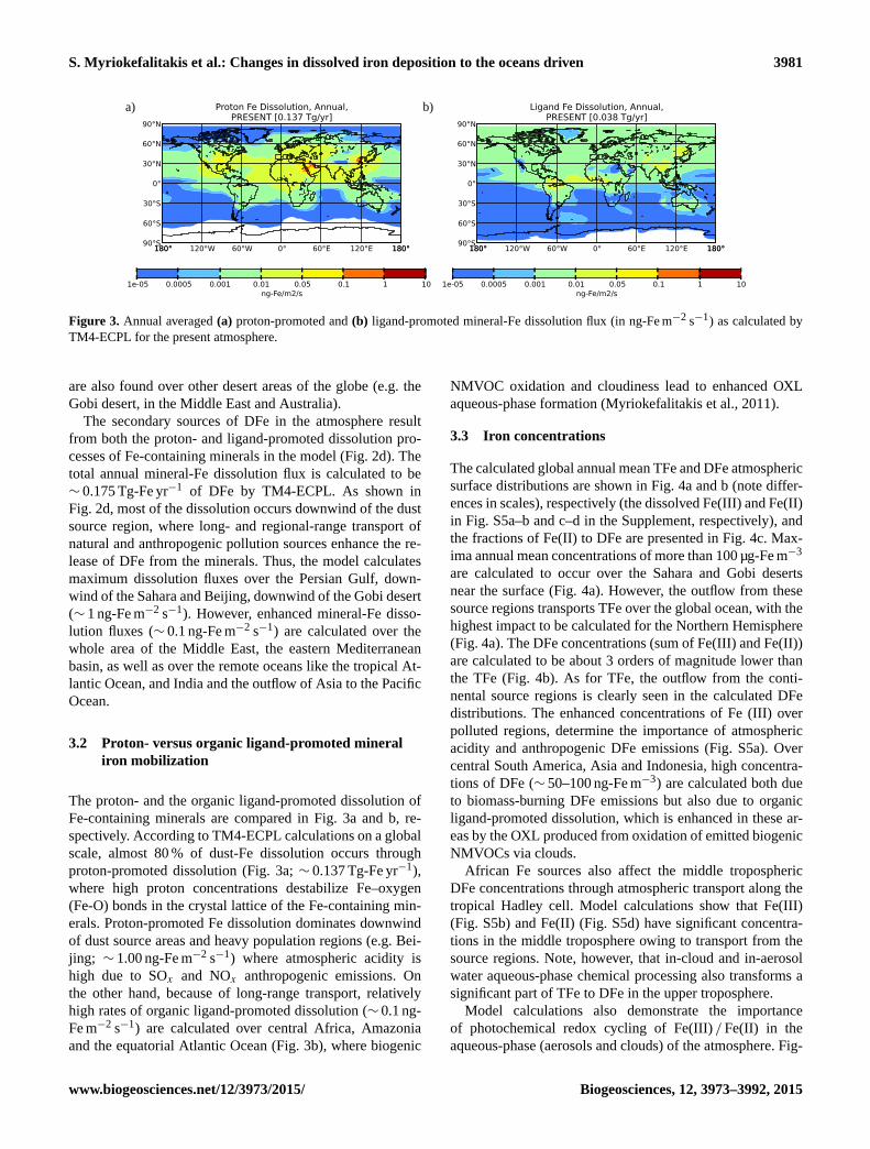
Figure 3. Annual averaged (a) proton-promoted and (b) ligand-promoted mineral-Fe dissolution flux (in ng-Fe m−2 s−1) as calculated by

TM4-ECPL for the present atmosphere.

are also found over other desert areas of the globe (e.g. the

Gobi desert, in the Middle East and Australia).

The secondary sources of DFe in the atmosphere result

from both the proton- and ligand-promoted dissolution pro-

cesses of Fe-containing minerals in the model (Fig. 2d). The

total annual mineral-Fe dissolution flux is calculated to be

∼ 0.175 Tg-Fe yr−1 of DFe by TM4-ECPL. As shown in

Fig. 2d, most of the dissolution occurs downwind of the dust

source region, where long- and regional-range transport of

natural and anthropogenic pollution sources enhance the re-

lease of DFe from the minerals. Thus, the model calculates

maximum dissolution fluxes over the Persian Gulf, down-

wind of the Sahara and Beijing, downwind of the Gobi desert

(∼ 1 ng-Fe m−2 s−1). However, enhanced mineral-Fe disso-

lution fluxes (∼ 0.1 ng-Fe m−2 s−1) are calculated over the

whole area of the Middle East, the eastern Mediterranean

basin, as well as over the remote oceans like the tropical At-

lantic Ocean, and India and the outflow of Asia to the Pacific

Ocean.

3.2 Proton- versus organic ligand-promoted mineral

iron mobilization

The proton- and the organic ligand-promoted dissolution of

Fe-containing minerals are compared in Fig. 3a and b, re-

spectively. According to TM4-ECPL calculations on a global

scale, almost 80 % of dust-Fe dissolution occurs through

proton-promoted dissolution (Fig. 3a; ∼ 0.137 Tg-Fe yr−1),

where high proton concentrations destabilize Fe–oxygen

(Fe-O) bonds in the crystal lattice of the Fe-containing min-

erals. Proton-promoted Fe dissolution dominates downwind

of dust source areas and heavy population regions (e.g. Bei-

jing; ∼ 1.00 ng-Fe m−2 s−1) where atmospheric acidity is

high due to SOx and NOx anthropogenic emissions. On

the other hand, because of long-range transport, relatively

high rates of organic ligand-promoted dissolution (∼ 0.1 ng-

Fe m−2 s−1) are calculated over central Africa, Amazonia

and the equatorial Atlantic Ocean (Fig. 3b), where biogenic

NMVOC oxidation and cloudiness lead to enhanced OXL

aqueous-phase formation (Myriokefalitakis et al., 2011).

3.3 Iron concentrations

The calculated global annual mean TFe and DFe atmospheric

surface distributions are shown in Fig. 4a and b (note differ-

ences in scales), respectively (the dissolved Fe(III) and Fe(II)

in Fig. S5a–b and c–d in the Supplement, respectively), and

the fractions of Fe(II) to DFe are presented in Fig. 4c. Max-

ima annual mean concentrations of more than 100 µg-Fe m−3

are calculated to occur over the Sahara and Gobi deserts

near the surface (Fig. 4a). However, the outflow from these

source regions transports TFe over the global ocean, with the

highest impact to be calculated for the Northern Hemisphere

(Fig. 4a). The DFe concentrations (sum of Fe(III) and Fe(II))

are calculated to be about 3 orders of magnitude lower than

the TFe (Fig. 4b). As for TFe, the outflow from the conti-

nental source regions is clearly seen in the calculated DFe

distributions. The enhanced concentrations of Fe (III) over

polluted regions, determine the importance of atmospheric

acidity and anthropogenic DFe emissions (Fig. S5a). Over

central South America, Asia and Indonesia, high concentra-

tions of DFe (∼ 50–100 ng-Fe m−3) are calculated both due

to biomass-burning DFe emissions but also due to organic

ligand-promoted dissolution, which is enhanced in these ar-

eas by the OXL produced from oxidation of emitted biogenic

NMVOCs via clouds.

African Fe sources also affect the middle tropospheric

DFe concentrations through atmospheric transport along the

tropical Hadley cell. Model calculations show that Fe(III)

(Fig. S5b) and Fe(II) (Fig. S5d) have significant concentra-

tions in the middle troposphere owing to transport from the

source regions. Note, however, that in-cloud and in-aerosol

water aqueous-phase chemical processing also transforms a

significant part of TFe to DFe in the upper troposphere.

Model calculations also demonstrate the importance

of photochemical redox cycling of Fe(III) /Fe(II) in the

aqueous-phase (aerosols and clouds) of the atmosphere. Fig-



a) b)

c)

Figure 4. Annual averaged (a) proton-promoted and (b) ligand-promoted mineral-Fe dissolution flux (in ng-Fe m−2 s−1) as calculated by

TM4-ECPL for the present atmosphere.

ure 4c shows the percentage contribution of Fe(II) to DFe as

computed by the model, denoting that the calculated Fe(II)

concentrations are an important part of DFe atmospheric bur-

den; regionally reaching up to 20 % of the total dissolved

mass far from the dust source areas e.g. the remote ocean.

This ratio also exceeds 10 % at several other locations around

the globe, in particular over the tropical Pacific and the

Southern Ocean; implying that chemical aging of dust due

to atmospheric processing and long-range transport enhances

the production of Fe(II) significantly. As also discussed in

Sect. 2.6, in relatively basic pH environments (e.g. the South-

ern Ocean due to the buffering capacity of sea-salt particles;

see Fig. S2a, b) and due to high OXL concentrations (e.g.

tropical Pacific ocean) the production of Fe(II) is favoured

(Fig. S4e and h, respectively). Thus, our model calculations

indicate that the enhanced fraction of Fe(II) over the remote

oceans (Fig. 4c), characterized by low concentrations of dust

and non-negligible OXL concentrations (see Fig. S3) due to

the aqueous-phase oxidation of organic compounds of ma-

rine origin NMVOCs (e.g. isoprene) could be attributed to

the production of ferrous oxalato complexes.

TM4-ECPL calculates a global TFe atmospheric burden of

∼ 0.857 Tg-Fe and almost 35 times lower atmospheric bur-

den of the DFe ∼ 0.024 Tg-Fe (∼ 0.023 Tg-Fe as Fe(III) and

∼ 0.001 Tg-Fe as Fe(II)). This also indicates the existence of

a large TFe reservoir that can be mobilized under favourable

conditions. The total SFe (Fig. S6a) is calculated to vary spa-

tially with minima over the dust sources (∼ 1 %) and max-

ima over the south equatorial regions (∼ 5 %). SFe due to

dust aerosols is attributed primarily to the atmospheric pro-

cessing and to the (low) initial dust solubility. These low SFe

values over dust source regions can be also explained by the

suppressed mineral-Fe dissolution because of the enhanced

buffering capacity (as well as the low water associated with

dust aerosols near their sources), the low acidity because of

the low amounts of acidic inorganic compounds from anthro-

pogenic pollution and the lack of organic ligands (e.g. OXL)

over large dust outbreaks (e.g. the Sahara) (Fig. S6b). On the

other hand, the model calculates higher SFe values (∼ 2.5–

5 %) of dust aerosols over regions characterized by low dust

concentrations but high amounts of anthropogenic pollution

(e.g. over the Indian Ocean). However, the co-existence of

relatively high dust concentrations and high amounts of an-

thropogenic pollutants tend to enhance mineral-Fe atmo-

spheric processing significantly and thus SFe (∼ 5 %), as

in the case of the Persian Gulf and eastern Mediterranean

(Fig. S6b). Fe-containing combustion aerosols of anthro-

pogenic origin (Fig. S6c) are also calculated to contribute

significantly to SFe (∼ 2.5 %) over high population regions

(e.g. the US, central Europe and China). Due to the long-

range transport in the Northern Hemisphere, enhanced SFe

is simulated also over the North Atlantic and Pacific oceans

(∼ 1.5 %). Additionally, biomass-burning processes are cal-

culated to increase SFe, especially over the Southern Hemi-



a) b)

c) d)

e)

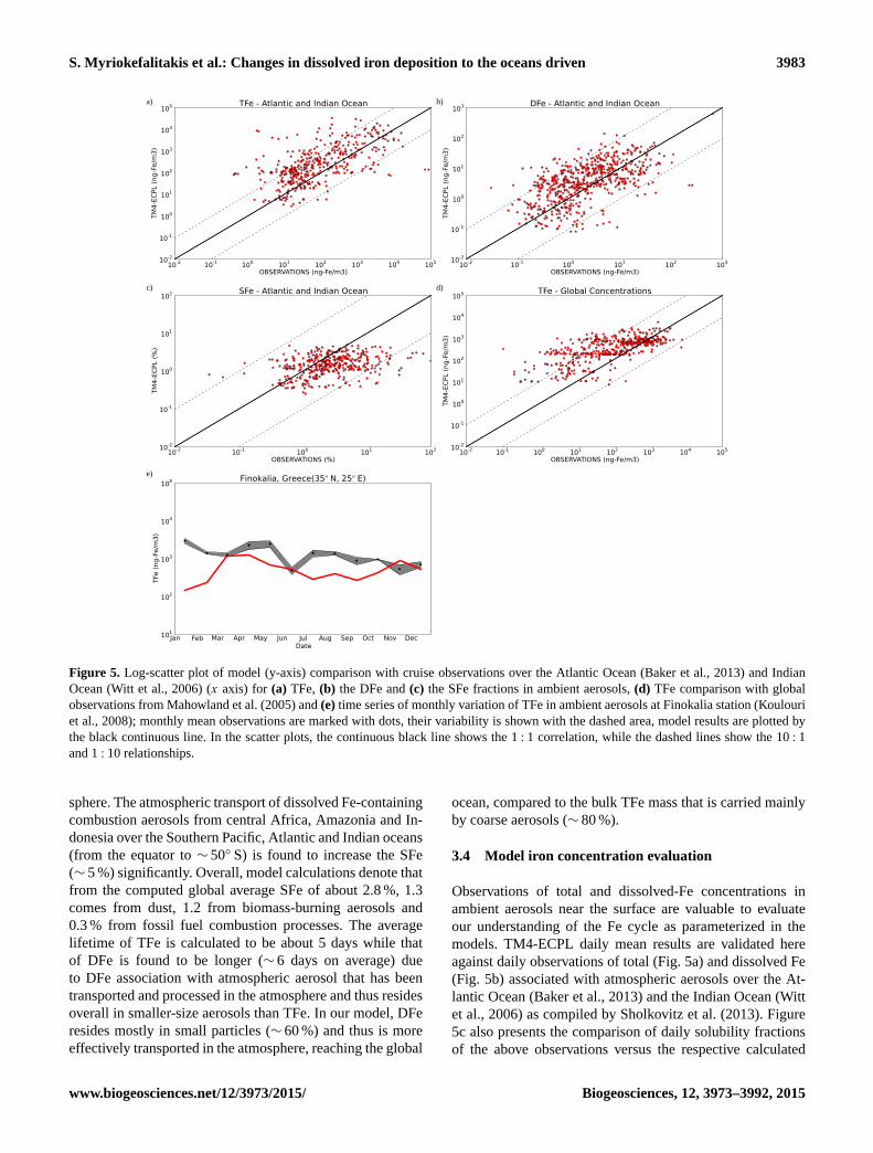
Figure 5. Log-scatter plot of model (y-axis) comparison with cruise observations over the Atlantic Ocean (Baker et al., 2013) and Indian

Ocean (Witt et al., 2006) (x axis) for (a) TFe, (b) the DFe and (c) the SFe fractions in ambient aerosols, (d) TFe comparison with global

observations from Mahowland et al. (2005) and (e) time series of monthly variation of TFe in ambient aerosols at Finokalia station (Koulouri

et al., 2008); monthly mean observations are marked with dots, their variability is shown with the dashed area, model results are plotted by

the black continuous line. In the scatter plots, the continuous black line shows the 1 : 1 correlation, while the dashed lines show the 10 : 1

and 1 : 10 relationships.

sphere. The atmospheric transport of dissolved Fe-containing

combustion aerosols from central Africa, Amazonia and In-

donesia over the Southern Pacific, Atlantic and Indian oceans

(from the equator to ∼ 50◦ S) is found to increase the SFe

(∼ 5 %) significantly. Overall, model calculations denote that

from the computed global average SFe of about 2.8 %, 1.3

comes from dust, 1.2 from biomass-burning aerosols and

0.3 % from fossil fuel combustion processes. The average

lifetime of TFe is calculated to be about 5 days while that

of DFe is found to be longer (∼ 6 days on average) due

to DFe association with atmospheric aerosol that has been

transported and processed in the atmosphere and thus resides

overall in smaller-size aerosols than TFe. In our model, DFe

resides mostly in small particles (∼ 60 %) and thus is more

effectively transported in the atmosphere, reaching the global

ocean, compared to the bulk TFe mass that is carried mainly

by coarse aerosols (∼ 80 %).

3.4 Model iron concentration evaluation

Observations of total and dissolved-Fe concentrations in

ambient aerosols near the surface are valuable to evaluate

our understanding of the Fe cycle as parameterized in the

models. TM4-ECPL daily mean results are validated here

against daily observations of total (Fig. 5a) and dissolved Fe

(Fig. 5b) associated with atmospheric aerosols over the At-

lantic Ocean (Baker et al., 2013) and the Indian Ocean (Witt

et al., 2006) as compiled by Sholkovitz et al. (2013). Figure

5c also presents the comparison of daily solubility fractions

of the above observations versus the respective calculated



Figure 6. Calculated present annual deposition (in ng-Fe m−2 s−1) for (a) TFe, (b) DFe, and the seasonal DFe deposition fluxes for (c)

December, January and February (DJF), (d) March, April and May (MAM), (e) June, July and August (JJA) and (f) September, October and

November (SON). In brackets (parentheses) the amounts of Fe deposition over the globe (only over oceans) are provided.

fractions by the model. In addition, Fe aerosol data compiled

by Mahowald et al. (2005) are compared with model results

in Fig. 5d. The seasonality of TFe in the eastern Mediter-

ranean as measured and compiled by Koulouri et al. (2008)

at Finokalia station (http://finokalia.chemistry.uoc.gr/) is also

compared to monthly model results (Fig. 5e).

The comparisons presented in Fig. 5 show that the model

reasonably simulates the observed concentration of total and

dissolved Fe in the ambient aerosols over oceans (scatter

plots in Fig. 5a, b and c). In the eastern Mediterranean, when

comparing to ambient aerosol observations at Finokalia mon-

itoring station (Fig. 5e), the model seems to underestimate

the observations of TFe with the largest differences calcu-

lated for January–February, May and July–September. These

are the periods of the year that Finokalia station can be

occasionally affected by strong dust outbreaks from Africa

(Kalivitis et al., 2007) that are better represented in the obser-

vations than in the model results due to their episodic charac-

ter. All evaluations (see Supplement Table S3) are based on

statistical parameters of correlation coefficient (R; Eq. S1),

normalized mean bias (NMB; Eq. S2), root mean square

error (RMSE; Eq. S3), and normalized mean error (NME;

Eq. S3).

3.5 Iron deposition

TM4-ECPL calculates that ∼ 37 Tg-Fe yr−1 of TFe are de-

posited to the Earth’s surface (Fig. 6a). The highest an-

nual deposition fluxes of TFe of ∼ 100 ng-Fe m−2 s−1 (i.e.

∼ 3.2 g-Fe m−2 yr−1) are calculated to occur over the Sahara

and Gobi deserts. Significant deposition fluxes up to∼ 10 ng-

Fe m−2 s−1 are also calculated at the outflow from these


http://finokalia.chemistry.uoc.gr/


0.00

4.00

8.00

12.00

16.00

20.00

Region 2 Region 3 Region 4 Region 5

Gm

ol-

Fe

/ A

MJ

Atlantic Ocean TFe DepositionApril-May-June

Baker et al., 2013

Johnson et al. 2010

Mahowald et al., 2009

This work

0.00

2.00

4.00

6.00

8.00

10.00


Gm

ol-

Fe

/ S

ON

Atlantic Ocean TFe DepositionSeptember-October-November

Baker et al., 2013

Johnson et al. 2010


This work

0.000

0.020

0.040

0.060

0.080

0.100

0.120

0.140


Gm

ol-

Fe

/ A

MJ

Atlantic Ocean DFe DepositionApril-May-June

Baker et al., 2013

Johnson et al. 2010


This work

0.000

0.050

0.100

0.150

0.200

0.250

0.300

0.350


Gm

ol-

Fe

/ S

ON

Atlantic Ocean DFe DepositionSeptember-October-November

Baker et al., 2013

Johnson et al. 2010


This work

a) b)

c) d)

Figure 7. Comparison of total Fe (TFe) and dissolved-Fe (DFe) input estimates to four Atlantic Ocean regions during the April–May–June

(AMJ; a, c) and September-October-November (SON; b, d) periods (in Gmol-Fe), as compiled by Baker et al. (2013).

source regions over the Atlantic and Pacific oceans. The com-

puted global DFe deposition is ∼ 0.496 Tg-Fe yr−1 of which

∼ 0.191 Tg-Fe yr−1 is deposited over the ocean (Fig. 6b).

This oceanic DFe deposition estimate is lower than an earlier

reported DFe deposition flux to the ocean of 0.26 Tg-Fe yr−1

(Johnson and Meskhidze, 2013). However, that study used

dust emissions of∼ 1900 Tg yr−1, about 60 % larger than the

dust sources in the present study (∼ 1091 Tg yr−1 for the year

2008). In addition, at least 50 % uncertainty was found to be

associated with the applied horizontal resolution of the model

in the calculated deposition fluxes, with higher fluxes calcu-

lated by the higher model resolution.

Figures 6c–f present the seasonal variability of DFe depo-

sition as calculated by TM4-ECPL (in parenthesis the depo-

sition fluxes over the oceans are also provided). The max-

imum global seasonal DFe deposition flux of ∼ 0.132 Tg-

Fe season−1 is calculated to occur during JJA (June–

July–August; Fig. 6e), followed by fluxes of ∼ 0.128 Tg-

Fe season−1 during DJF (December–January–February;

Fig. 6c) and ∼ 0.127 Tg-Fe season−1 during MAM (March–

April–May; Fig. 6d). The enhanced photochemistry during

summertime over the Northern Hemisphere increases the at-

mospheric acidity due to NOx and SOx oxidation, and thus

enhances proton-dissolution of mineral dust. However, com-

bustion emissions from biomass burning and oil combustion

of anthropogenic origin also contribute significantly to the

DFe tropospheric concentrations. Moreover, OXL aqueous-

phase formation and therefore organic ligand-promoted Fe

dissolution is favoured due to the high biogenic NMVOC

emissions during the warm season (Myriokefalitakis et al.,

2011). On the contrary, during SON (September–October–

November; Fig. 6f) the model calculates lower DFe depo-

sition fluxes, of ∼ 0.109 Tg-Fe season−1, due to the weaker

photochemical activity and therefore the lower Fe dissolution

fluxes both from proton- and organic ligand-promoted disso-

lution. Note, also, that most dust and TFe emissions occur in

the mid-latitudes of the Northern Hemisphere where the ma-

jority of anthropogenic emissions of acidity precursors also

occur (Fig. S1).

3.6 Model iron deposition evaluation

In Fig. 7, TM4-ECPL deposition fluxes of TFe and DFe

(in this work) are compared to the estimates over four At-

lantic Ocean regions (Fig. S7a–d) based on the observations

of Baker et al. (2013) as well as the deposition fields from

the modelling studies of Mahowald et al. (2009) and John-

son et al. (2010) as compiled and presented by Baker et al.

(2013). Both of these modelling studies assumed a constant

Fe content of 3.5 % in dust and a proton-promoted Fe disso-

lution. DFe deposition fluxes have been calculated for four



a) b)

c) d)

Figure 8. The percentage differences of PAST (a, c, e) and FUTURE (b, d, f) simulations from the PRESENT simulation for (a, b) proton-

promoted/total mineral-Fe dissolution fraction and (c, d) ligand-promoted/total mineral-Fe dissolution fraction.

regions, as described in Baker et al. (2013), with Region 2

corresponding to North Atlantic dry regions, Region 3 corre-

sponding to intertropical convergence zone (ITCZ), Region 4

to South Atlantic dry regions and Region 5 to South Atlantic

storm rainfall (Fig. S7a–d).

In the South Atlantic (Region 4) during AMJ (April–

May–June) TM4-ECPL calculations of TFe deposition show

a broad agreement with the measurements and also agree

with the other modelling studies, when taking the large un-

certainty associated with these estimates into account. On

the other hand, the model overestimates the measurements

of TFe in Region 2 and Region 3 during AMJ similarly

to the modelling study by Mahowald et al. (2009). These

regions are both strongly affected by Sahara dust outflow;

thus the model overestimates TFe observations by Baker et

al. (2013), while DFe observations are much better captured

by the model. This could be due to a longer lifetime of TFe

in the model than in the atmosphere, resulting from smaller

size distributions of TFe in the model than in reality. Dur-

ing SON (Fig. 7b), TM4-ECPL overestimates the measured

values from Baker et al. (2013) similarly to the modelling

study by Mahowald et al. (2009). For Region 4 during SON,

the model agrees well with the Baker et al. (2013) estimates

and calculates TFe deposition fluxes, which were lower com-

pared to Mahowald et al. (2009) but very close to the esti-

mation by Johnson et al. (2010). Overall, TM4-ECPL model

overestimates the observed DFe deposition over Regions 2,

3 and 4 during both studied periods, while it underestimates

DFe deposition over Region 5 similarly to other model esti-

mates (Fig. 7c, d).

4 Sensitivity of dissolved iron to air-pollutants

The response of mineral-Fe dissolution to the changes in

emissions is assessed here by comparing simulations per-

formed using anthropogenic and biomass burning past and

future emissions (see Sect. 2). Atmospheric acidity strongly

depends on SOx and NOx anthropogenic emissions, and Fe

solubility is impacted by atmospheric acidity as discussed

above. Mineral dissolution is therefore expected to be sig-

nificantly affected by anthropogenic emissions. Iron anthro-

pogenic and biomass-burning emissions also vary, as shown

in Table 1 and explained in Sect. 2.3. Note, however, that me-

teorology, dust emissions and biogenic NMVOC emissions

(and thus OXL precursors from biogenic sources) are kept

constant for both PAST and FUTURE simulations, corre-

sponding to the year 2008 (i.e. PRESENT simulation). Thus,

the computed changes for species that regulate the mineral-

Fe proton and ligand dissolution (e.g. SO2−4 , NH+4 , NO−3 and

OXL), as presented in Fig. S8, are due to the respective an-

thropogenic and biomass-burning emission differences be-

tween PAST, PRESENT and FUTURE simulations.



4.1 Past and future changes in iron dissolution

For the PAST simulation, the anthropogenic emissions (e.g.

NOx , NHx and SOx) are a factor of 5–10 lower than present-

day emissions (Lamarque et al., 2010). Thus, compared to

the present day, the model calculates significant changes in

the aerosol-phase pH in the PAST simulation with less acidic

(aerosol and cloud) pH over the surface Northern Hemi-

sphere oceans but a more acidic pH over Europe due to ex-

tensive coal combustion in 1850 (Fig. S2e, g, i). The FU-

TURE simulation projects, in general, a less acidic aerosol

pH (Fig. S2f, h, j) when compared to the PRESENT simu-

lation, owing to lower NOx and SOx emissions. Indeed, for

the FUTURE simulation, anthropogenic emissions for most

of the continental areas are projected to be lower than the

present day and projected to almost return to pre-1980 levels

due to air quality regulations (Lamarque et al., 2013).

Past and future changes of the atmospheric acidity

(Fig. S2) have a significant effect on mineral-Fe dissolu-

tion (Fig. 8a and b, respectively). For the PAST simula-

tion, the model calculates about 80 % lower proton-promoted

mineral-Fe dissolution (∼ 0.025 Tg-Fe yr−1) compared to the

PRESENT simulation (∼ 0.137 yr−1). As far as the FUTURE

simulation is concerned, proton-promoted mineral-Fe disso-

lution (∼ 0.036 Tg-Fe yr−1) is also projected to be about 3

times lower than at present. In contrast to these changes due

to atmospheric acidity, a higher contribution of organic lig-

and to the total mineral-Fe dissolution is computed; for the

PAST and FUTURE simulations, the model calculates higher

global-scale organic ligand-promoted mineral-Fe dissolution

(∼ 0.040 and ∼ 0.045 Tg-Fe yr−1, respectively) compared to

the PRESENT (∼ 0.038 yr−1). Thus, the contribution of the

organic ligand-promoted mineral-Fe dissolution process to

the total dissolution flux is calculated to show an inverse pat-

tern compared to the proton-promoted one (Fig. 8c, d). Dif-

ferences in the pH of atmospheric (aerosol and cloud) wa-

ter and oxidant levels can significantly affect OXL aqueous-

phase chemical production (Myriokefalitakis et al., 2011).

According to TM4-ECPL calculations, the increase in OXL

levels enhances the organic ligand-promoted mineral-Fe dis-

solution in remote oceanic regions with very low dust load.

However, dust load over the remote oceans could increase if

dust outbreaks become more important in the future (Goudie,

2009). One other aspect of the organic ligand-promoted

mineral-Fe dissolution is also the effect on the speciation

of dissolved and bioavailable Fe. According to the chem-

ical scheme used in this work, the production of Fe(II) -

oxalato complexes significantly increases the ferrous content

in the DFe, in contrast to the proton-promoted mineral-Fe

dissolution where Fe(III) complexes dominate total DFe pro-

duction. Indeed, when only the proton-promoted Fe dissolu-

tion is considered in our model, the ferrous complexes are

produced during the day, when the Fe(III) is converted into

Fe(II) as a result of the Fe(III) photolysis (e.g. Deguillaume

et al., 2004). However, when the organic ligand Fe dissolu-

tion is taken into account, the Fe(II) is increased, since there

is production of ferrous complexes even under dark condi-

tions. This may also explain the observed high Fe(II) con-

tent compared to Fe(III) in the DFe in precipitation over the

Mediterranean (Theodosi et al., 2010). However, our model

calculates much lower Fe(II) content in DFe (Fig. 4c) com-

pared to that study, indicating a model underestimate of the

Fe(II) source, potentially associated with the organic ligand-

promoted contribution to DFe. TM4-ECPL calculates that

the decrease in the atmospheric acidity both in the PAST and

in the FUTURE compared to the PRESENT simulations in-

creases the importance of organic ligand mineral-Fe dissolu-

tion and thus leads to a significant enhancement of the Fe(II)

surface concentrations and thus its content in DFe (Fig. S9a,

b) and a simultaneous reduction of Fe(III) (Fig. S9c, d).

4.2 Past and future changes in iron deposition

The model calculates a DFe deposition flux of ∼ 0.213 Tg-

Fe yr−1 (with ∼ 0.063 Tg-Fe yr−1 over oceans) in the PAST

that is about half (to one-third over the oceans) (Fig. S9e,

negative differences) compared to PRESENT (∼ 0.496 with

∼ 0.191 Tg-Fe yr−1 over oceans). On the other hand, FU-

TURE DFe deposition is calculated to be ∼ 0.369 Tg-

Fe yr−1 (with ∼ 0.136 Tg-Fe yr−1 over oceans) which is

about 25 % lower than the simulated global PRESENT depo-

sition (Fig. S9f). This can be explained by lower amounts of

combustion DFe-containing aerosols simulated to be emitted

in the PAST (∼ 0.011 Tg-Fe yr−1 from fossil fuel combus-

tion and∼ 0.013 Tg-Fe yr−1 from biomass-burning aerosols)

compared to the PRESENT simulation (∼ 0.070 Tg-Fe yr−1

from fossil fuel combustion and ∼ 0.127 Tg-Fe yr−1 from

biomass-burning aerosols), as well as in the FUTURE

(∼ 0.013 Tg-Fe yr−1 from fossil fuel combustion) compared

to the PRESENT simulation. However, higher emissions of

biomass-burning Fe-containing aerosols are projected for the

FUTURE (∼ 0.155 Tg-Fe yr−1) (see also Table 1) that coun-

teract the projected lower Fe emissions contained in fossil

fuel aerosols and the weaker mineral-Fe dissolution for the

FUTURE simulation. The weaker acidification of mineral

dust in the past and future, compared to the PRESENT atmo-

sphere (Fig. S7e, g, i and f, h, j) can also be seen in SO2−4 and

NO−3 surface concentrations, by the negative changes from

the present day, shown in Fig. S8a, c and b, and d.

4.3 Biogeochemical implications

The determination of iron solubility is important to under-

stand the carbon biogeochemical cycle. Okin et al. (2011)

have shown that in HNLC areas, atmospheric deposition of

Fe to the surface ocean could account for about 50 % of car-

bon fixation, although they pointed to the large uncertain-

ties in the speciation and solubility of deposited Fe that are

associated with these estimates. Thus, the impact of Fe on

ocean productivity, and subsequently on Earth’s climate sys-



a) b)

c) d)

Figure 9. Calculated present annual deposition over oceans (in ng-Fe m−2 s−1; in brackets (parentheses) the amounts of Fe deposition over

oceans (only over HNLC regions are provided)) for (a) TFe and (b) DFe, and the percentage (%) differences in DFe deposition of (c) PAST

and (d) FUTURE simulations from the PRESENT simulation.

tem, is expected to be most important in HNLC areas such

as the Southern Ocean (Boyd et al., 2000). However, be-

cause the DFe deposited from the atmosphere to the sur-

face water follows the water flow inside the ocean, atmo-

spheric deposition impact is expected to be geographically

extended compared to the surfaces where this deposition oc-

curs and can be only evaluated by an ocean biogeochemical

model. For the characterization of HNLC oceanic regions in

this study, the annual mean global NO−3 surface water con-

centrations from the LEVITUS94 World Ocean Atlas (http:

//iridl.ldeo.columbia.edu/SOURCES/.LEVITUS94/) and the

monthly chlorophyll a (Chl a) concentrations MODIS re-

trievals taken into account in the model (Myriokefalitakis et

al., 2010) for the year 2008 are used. The model grid boxes

corresponding to HNLC waters (Fig. S7e) are defined here

based on the co-occurrence of surface seawater NO−3 con-

centrations of > 4 µM (Duce et al., 2008) and Chl a concen-

trations of < 0.1 mg m−3 (Boyd et al., 2007).

The deposition fluxes of TFe and DFe over oceans are

presented in Fig. 9a and b, respectively. The model calcu-

lates that ∼ 1.052 Tg-Fe yr−1 of TFe are deposited over the

HNLC ocean with the maximum deposition fluxes calcu-

lated over the North Pacific Ocean (∼ 5–10 ng-Fe m−2 s−1)

and the lowest over the Southern Ocean (∼ 0.05–0.5 ng-

Fe m−2 s−1). The same pattern is also calculated for the DFe

deposition, with maximum DFe deposition fluxes over the

equatorial Atlantic Ocean (∼ 0.5 ng-Fe m−2 s−1), relatively

high deposition fluxes over the North Pacific Ocean (∼ 0.01–

0.05 ng-Fe m−2 s−1) and lower over the Southern Ocean (up

to ∼ 0.005 ng-Fe m−2 s−1). TM4-ECPL calculates a deposi-

tion flux of ∼ 0.033 Tg-Fe yr−1 of DFe over the HNLC wa-

ters which represents ∼ 17 % of the total oceanic DFe depo-

sition flux and ∼ 7 % of the global one.

The percentage differences of calculated PRESENT DFe

deposition fluxes over oceans from the PAST and FUTURE

simulations are depicted in Fig. 9c and d, respectively. The

model in general calculates for both PAST and FUTURE

simulations lower DFe deposition fluxes over oceans. DFe

deposition fluxes are calculated to be ∼ 80 % higher in the

PRESENT than in the PAST simulation (Fig. 9c), which can

be attributed both to the increase of (i) mineral-Fe dissolu-

tion (almost 3-fold) and (ii) primary DFe emission (from

both fossil fuel combustion (6-fold) and biomass-burning

sources (almost an order of magnitude)). Furthermore, based

on emission projections following air quality legislation, de-

creases of about 30–60 % in DFe deposition are calculated

for the FUTURE simulation over the North Pacific and At-

lantic oceans, the Arabian Sea, the Bay of Bengal and the

eastern Mediterranean Sea and lower reductions (less than

20 %) over the remote tropical Pacific and Atlantic oceans

and the Southern Ocean. These smaller changes from the

PRESENT simulation calculated for the FUTURE (about a

45 % reduction globally) than for the PAST (almost a 3-fold

change globally) are attributed to the projected increase of Fe


http://iridl.ldeo.columbia.edu/SOURCES/ .LEVITUS94/

http://iridl.ldeo.columbia.edu/SOURCES/ .LEVITUS94/


biomass-burning emissions (about 20 %) that partially coun-

terbalance the more than 5-fold reduction in anthropogenic

emissions of Fe. Overall, these sensitivity PAST–FUTURE

simulations clearly support that changes in (i) atmospheric

acidity and (ii) Fe combustion sources, both driven by an-

thropogenic pollutant emissions, affect DFe deposition over

the oceans significantly, and therefore they have the potential

to also perturb open-ocean phytoplankton growth and thus

the carbon biogeochemical cycling.

5 Conclusions

Primary Fe emissions from dust and combustion sources

(fossil fuel and biomass burning) of TFe and DFe, as well

as the atmospheric processing by proton- and organic ligand-

promoted mineral-Fe dissolution together with aqueous-

phase photochemical reactions between oxidation states of

Fe (III/II), are taken into account in the state-of-the-art chem-

istry transport model TM4-ECPL. The model calculates, for

present-day conditions, an atmospheric Fe dissolution flux

of ∼ 0.175 Tg-Fe yr−1 of which ∼ 22 % is attributed to the

impact of organic ligands on the Fe cycle. The atmospheric

burden of DFe is calculated to be ∼ 0.024 Tg-Fe and the

dissolved-Fe annual deposition flux over the oceans to be

∼ 0.119 Tg-Fe yr−1. SFe (global mean of about 2.8 %) is cal-

culated to vary spatially with minima over the dust sources

(∼ 1 %). This global mean solubility of Fe, originates from

dust (1.3 %), biomass-burning aerosols (1.3 %) and fossil

fuel combustion (0.3 %). Note that these model estimates

are associated with large uncertainties in the kinetics of Fe

dissolution as well as the primary total and dissolved-Fe

emissions. As earlier explained, model results depend on

model resolution but more importantly depend on assump-

tions made in the model, such as neglecting any organic lig-

and dissolution of Fe in aerosol water and treating biomass-

burning and fossil fuel-burning DFe as primary.

Sensitivity simulations show that increases in anthro-

pogenic and biomass burning-emissions since 1850 resulted

in both enhanced Fe combustion emissions and a more acidic

environment and thus more than double DFe deposition

(∼ 0.213 Tg-Fe yr−1 in the year 1850 against ∼ 0.496 Tg-

Fe yr−1 in the present day). Air-quality regulations are pro-

jected to decrease anthropogenic emissions and thus at-

mospheric acidity in 2100. Our model results show a 5-

fold decrease in Fe emissions from anthropogenic combus-

tion sources (∼ 0.013 Tg-Fe yr−1 in the year 2100 against

∼ 0.070 Tg-Fe yr−1 in the present day), and about 45 %

reduction in mineral-Fe dissolution (∼ 0.078 Tg-Fe yr−1)

compared to the present day (∼ 0.175 Tg-Fe yr−1), while

DFe biomass-burning emissions are enhanced by 20 %

(∼ 0.155 Tg-Fe yr−1 in the year 2100 against ∼ 0.127 Tg-

Fe yr−1 in the present day). Overall, the model calculates

a global DFe deposition of ∼ 0.369 Tg-Fe yr−1 for the year

2100 that is ∼ 25 % lower than the present-day deposition.

Focusing on oceanic regions, an increase in DFe de-

position of ∼ 3 times is calculated for the last 150 years

(0.063 Tg-Fe yr−1 in the year 1850 against ∼ 0.191 Tg-

Fe yr−1 in the present day) but a decrease of ∼ 30 % over

HNLC oceans is projected for the future (0.024 Tg-Fe yr−1

in the year 2100 against ∼ 0.033 Tg-Fe yr−1 in the present

day). In view of the importance of Fe as a micronutrient for

marine ecosystems, the calculated changes in Fe-containing

aerosol solubility due to air-quality changes, indicate the ne-

cessity of the implementation of comprehensive mineral-Fe

dissolution processes as well as Fe combustion emissions

in coupled climate-biogeochemistry models to account for

feedbacks between climate and biogeochemical cycles.

The Supplement related to this article is available online

at doi:10.5194/bg-12-3973-2015-supplement.

Acknowledgements. This research has been co-financed by the

European Union (European Social Fund – ESF) and Greek national

funds through the Operational Program “Education and Lifelong

Learning” of the National Strategic Reference Framework (NSRF)

Research Funding Program: ARISTEIA – PANOPLY (Pollution

Alters Natural aerosol composition: implications for Ocean

Productivity, cLimate and air qualitY) grant. We would like to

thank Z. Shi and S. Nickovic for fruitful discussions and the two

anonymous reviewers for careful reading of the manuscript and

useful comments.

Edited by: L. Bopp

References

Baker, A. R., Adams, C., Bell, T. G., Jickells, T. D., and Ganzeveld,

L.: Estimation of atmospheric nutrient inputs to the Atlantic

Ocean from 50◦ N to 50◦ S based on large-scale field sampling:

Iron and other dust-associated elements, Global Biogeochem.

Cy., 27, 755–767, 2013.

Bonneville, S., Vancappellen, P., and Behrends, T.: Microbial reduc-

tion of iron(III) oxyhydroxides: effects of mineral solubility and

availability, Chem. Geol., 212, 255–268, 2004.

Boyd, P. W., Watson, A. J., Law, C. S., Abraham, E. R., Trull, T.,

Murdoch, R., Bakker, D. C., Bowie, A. R., Buesseler, K. O.,

Chang, H., Charette, M., Croot, P., Downing, K., Frew, R., Gall,

M., Hadfield, M., Hall, J., Harvey, M., Jameson, G., LaRoche,

J., Liddicoat, M., Ling, R., Maldonado, M. T., McKay, R. M.,

Nodder, S., Pickmere, S., Pridmore, R., Rintoul, S., Safi, K., Sut-

ton, P., Strzepek, R., Tanneberger, K., Turner, S., Waite, A. and

Zeldis, J.: A mesoscale phytoplankton bloom in the polar South-

ern Ocean stimulated by iron fertilization., Nature, 407, 695–

702, 2000.

Boyd, P. W., Strzepek R., Takeda S.,Wong, C. S., and McKay, R.

M.: The evolution and termination of an iron-induced mesoscale

bloom in the northeast subarctic Pacific, Limnol. Oceanogr., 50,

1872–1886, 2005.


http://dx.doi.org/10.5194/bg-12-3973-2015-supplement


Boyd, P. W., Jickells, T., Law, C. S., Blain, S., Boyle, E. A., Bues-

seler, K. O., Coale, K. H., Cullen, J. J., de Baar, H. J. W., Follows,

M., Harvey, M., Lancelot, C., Levasseur, M., Owens, N. P. J., Pol-

lard, R., Rivkin, R. B., Sarmiento, J., Schoemann, V., Smetacek,

V., Takeda, S., Tsuda, A., Turner, S., and Watson A. J.: Mesoscale

Iron Enrichment Experiments 1993–2005: Synthesis and Future

Directions, Science, 315, 5812, doi:10.1126/science.1131669,

2007.

Carlton, A. G., Turpin, B. J., Altieri, K. E., Seitzinger, S., Reff, A.,

Lim, H.-J., and Ervens, B.: Atmospheric oxalic acid and SOA

production from glyoxal: Results of aqueous photooxidation ex-

periments, Atmos. Environ., 41, 7588–7602, 2007.

Chen, H. and Grassian, V. H.: Iron dissolution of dust source ma-

terials during simulated acidic processing: the effect of sulfuric,

acetic, and oxalic acids., Environ. Sci. Technol., 47, 10312–21,

2013.

Daskalakis, N., Myriokefalitakis, S., and Kanakidou, M.: Sensi-

tivity of tropospheric loads and lifetimes of short lived pollu-

tants to fire emissions, Atmos. Chem. Phys., 15, 3543–3563,

doi:10.5194/acp-15-3543-2015, 2015

Dee, D. P., Uppala, S. M., Simmons, A. J., Berrisford, P., Poli,

P., Kobayashi, S., Andrae, U., Balmaseda, M. A., Balsamo, G.,

Bauer, P., Bechtold, P., Beljaars, A. C. M., van de Berg, L., Bid-

lot, J., Bormann, N., Delsol, C., Dragani, R., Fuentes, M., Geer,

A. J., Haimberger, L., Healy, S. B., Hersbach, H., Hólm, E. V.,

Isaksen, L., Kållberg, P., Köhler, M., Matricardi, M., McNally,

A. P., Monge-Sanz, B. M., Morcrette, J. J., Park, B. K., Peubey,

C., de Rosnay, P., Tavolato, C., Thépaut, J. N., and Vitart, F.: The

ERA-Interim reanalysis: configuration and performance of the

data assimilation system, Q. J. Roy. Meteor. Soc., 137, 553–597,

2011.

Deguillaume, L., Leriche, M., Monod, A., and Chaumerliac, N.:

The role of transition metal ions on HO x radicals in clouds: a

numerical evaluation of its impact on multiphase chemistry, At-

mos. Chem. Phys., 4, 95–110, doi:10.5194/acp-4-95-2004, 2004.

Dentener, F., Kinne, S., Bond, T., and Boucher, O.: Emissions of pri-

mary aerosol and precursor gases in the years 2000 and 1750 pre-

scribed data-sets for AeroCom, Atmos. Chem. Phys., 6, 4321–

4344, doi:10.5194/acp-6-4321-2006, 2006.

Duce, R., A. LaRoche, J., Altieri, K., Arrigo, K.R., Baker, A.

R., Capone, D. G., Cornell, S.,Dentener, F., Galloway, J.,

Ganeshram, R. S., Geider, R. J., Jickells, T., Kuypers, M. M.,

Langlois, R., Liss, P. S., Liu, S. M., Middelburg, J. J., Moore,

C. M., Nickovic, S., Oschlies, A., Pedersen, T., Prospero, J.,

Schlitzer, R., Seitzinger, S., Sorensen, L. L., Uematsu, M., Ulloa,

O., Voss, M., Ward, B., and Zamora, L.: Impacts of Atmospheric

Anthropogenic Nitrogen on the Open Ocean, Science, 320, 5878,

doi:10.1126/science.1150369, 2008.

Ervens, B., George, C., Williams, J. E., Buxton, G. V., Salmon, G.

A., Bydder, M., Wilkinson, F., Dentener, F., Mirabel, P., Wolke,

R., and Herrmann, H: CAPRAM 2.4 (MODAC mechanism): An

extended and condensed tropospheric aqueous phase mechanism

and its application, J. Geophys. Res., 108, 1–21, 2003.

Falkowski P., Scholes R.J., Boyle E., Canadell J., Canfield, D.,

Elser, J., Gruber, N., Hibbard, K., Högberg, P., Linder, S.,

Mackenzie, F. T., Moore III, B., Pedersen, T., Rosenthal, Y.,

Seitzinger, S., Smetacek, V., and Steffen W.: The Global Carbon

Cycle: A Test of Our Knowledge of Earth as a System, Science,

290, 291–296, 2000.

Fan, S.-M.: Impact of air pollution on wet deposition of

mineral dust aerosols, Geophys. Res. Lett., 31, L02104,

doi:10.1029/2003GL018501, 2004.

Formenti, P., Rajot, J. L., Desboeufs, K., Caquineau, S., Chevail-

lier, S., Nava, S., Gaudichet, A., Journet, E., Triquet, S., Al-

faro, S., Chiari, M., Haywood, J., Coe, H., and Highwood,

E.: Regional variability of the composition of mineral dust

from western Africa: results from the AMMA SOP0/DABEX

and DODO field campaigns, J. Geophys. Res., 113, D00C13,

doi:10.1029/2008JD009903, 2008.

Formenti, P., Caquineau, S., Desboeufs, K., Klaver, A., Chevail-

lier, S., Journet, E., and Rajot, J. L.: Mapping the physico-

chemical properties of mineral dust in western Africa: miner-

alogical composition, Atmos. Chem. Phys., 14, 10663–10686,

doi:10.5194/acp-14-10663-2014, 2014.

Fountoukis, C. and Nenes, A.: ISORROPIA II: a computa-

tionally efficient thermodynamic equilibrium model for K+–

Ca2+–Mg2+–NH+4

–Na+–SO2−4

–NO−3

–Cl−–H2O aerosols: At-

mos. Chem. Phys., 7, 4639–4659, doi:10.5194/ acp-7-4639-

2007, 2007.

Goudie, S.: Dust storms: Recent developments, J. Environ. Man.,

90, 89–94, 2009.

Granier, C., Guenther, A., Lamarque, J., Mieville, A., Muller, J.,

Olivier, J., Orlando, J., Peters, J., Petron, G., Tyndall, G., and

Wallens, S.: POET, a database of surface emissions of ozone

pre-cursors, available at: http://www.pole-ether.fr/eccad (last ac-

cess: December 2015), ECCAD-Ether Database, 2005.Granier,

C., Guenther, A., Lamarque, J., Mieville, A., Muller, J., Olivier,

J., Orlando, J., Peters, J., Petron, G., Tyndall, G., and Wallens,

S.: POET, a database of surface emissions of ozone precursors,

available at: http://www.aero.jussieu.fr/projet/ACCENT/POET.

php, 2005.

Huneeus, N., Schulz, M., Balkanski, Y., Griesfeller, J., Prospero,

J., Kinne, S., Bauer, S., Boucher, O., Chin, M., Dentener, F.,

Diehl, T., Easter, R., Fillmore, D., Ghan, S., Ginoux, P., Grini,

A., Horowitz, L., Koch, D., Krol, M. C., Landing, W., Liu, X.,

Mahowald, N., Miller, R., Morcrette, J.-J., Myhre, G., Penner,

J., Perlwitz, J., Stier, P., Takemura, T., and Zender, C. S.: Global

dust model intercomparison in AeroCom phase I, Atmos. Chem.

Phys., 11, 7781–7816, doi:10.5194/acp-11-7781-2011, 2011.

Ito, A.: Global modeling study of potentially bioavailable iron in-

put from shipboard aerosol sources to the ocean, Global Bio-

geochem. Cy., 27, 1–10, 2013.

Ito, A.: Atmospheric Processing of Combustion Aerosols as a

Source of Bioavailable Iron, Environ. Sci. Technol. Lett., 2, 70–

75, doi:10.1021/acs.estlett.5b00007, 2015.

Ito, A. and Feng, Y.: Role of dust alkalinity in acid mobilization of

iron, Atmos. Chem. Phys., 10, 9237–9250, doi:10.5194/acp-10-

9237-2010, 2010.

Ito, A. and Xu, L.: Response of acid mobilization of iron-containing

mineral dust to improvement of air quality projected in the future,

Atmos. Chem. Phys., 14, 3441–3459, doi:10.5194/acp-14-3441-

2014, 2014.

Jeuken, A, Veefkind, J.P., Dentener, F., Metzger, S., and Roble Gon-

zalez, C.: Simulation of the aerosol optical depth over Europe for

August 1997 and a comparison with observations, J. Geophys.

Res., 106, 28295–28311, 2001.

Jickells, T. D. and Spokes, L. J.: Atmospheric iron inputs to the

oceans, in: The Biogeochemistry of Iron in Seawater, edited by:


http://dx.doi.org/10.1126/science.1131669

http://dx.doi.org/10.5194/acp-15-3543-2015



http://dx.doi.org/10.1126/science.1150369

http://dx.doi.org/10.1029/2003GL018501

http://dx.doi.org/10.1029/2008JD009903


http://dx.doi.org/10.5194/ acp-7-4639-2007

http://dx.doi.org/10.5194/ acp-7-4639-2007

http://www.pole-ether.fr/eccad

http://www.aero.jussieu.fr/projet/ACCENT/POET.php

http://www.aero.jussieu.fr/projet/ACCENT/POET.php


http://dx.doi.org/10.1021/acs.estlett.5b00007






Turner, D. R. and Hunter, K., SCOR/IUPAC Series, John Wiley

& Sons, New York, ISBN: 978-0-471-49068-5, 85–121, 2001.

Johnson, M. S. and Meskhidze, N.: Atmospheric dissolved iron de-

position to the global oceans: effects of oxalate-promoted Fe

dissolution, photochemical redox cycling, and dust mineralogy,

Geosci. Model Dev., 6, 1137–1155, doi:10.5194/gmd-6-1137-

2013, 2013.

Johnson, M. S., Meskhidze, N., Solmon, F., Gasso, S., Chuang,

P. Y., Gaiero, D. M., Yantosca, R. M., Wu, S., Wang, Y.,

and Carouge, C.: Modeling dust and soluble iron deposition

to the South Atlantic Ocean, J. Geophys. Res., 115, D15202,

doi:10.1029/2009JD013311, 2010.

Kalivitis, N., Gerasopoulos, E., Vrekoussis, M., Kouvarakis, G.,

Kubilay, N., Hatzianastassiou, N., Vardavas, I., and Mihalopou-

los, N.: Dust transport over the Eastern Mediterranean derived

from TOMS, AERONET and surface measurements, J. Geophys.

Res., 112, D03202, doi:10.1029/2006JD007510, 2007.

Koulouri, E., Saarikoski, S., Theodosi, C., Markaki, Z., Gerasopou-

los, E., Kouvarakis, G., Mäkelä, T., Hillamo, R., and Mihalopou-

los, N.: Chemical composition and sources of fine and coarse

aerosol particles in the Eastern Mediterranean, Atmos. Environ.,

42, 6542–6550, 2008.

Kraemer, S. M.: Iron oxide dissolution and solubility in the presence

of siderophores, Aquat. Sci.-Res. Acr. Bound., 66, 3–18, 2004.

Lamarque, J.-F., Bond, T. C., Eyring, V., Granier, C., Heil, A.,

Klimont, Z., Lee, D., Liousse, C., Mieville, A., Owen, B.,

Schultz, M. G., Shindell, D., Smith, S. J., Stehfest, E., Van Aar-

denne, J., Cooper, O. R., Kainuma, M., Mahowald, N., Mc-

Connell, J. R., Naik, V., Riahi, K., and van Vuuren, D. P.: His-

torical (1850–2000) gridded anthropogenic and biomass burning

emissions of reactive gases and aerosols: methodology and ap-

plication, Atmos. Chem. Phys., 10, 7017–7039, doi:10.5194/acp-

10-7017-2010, 2010.

Lamarque, J.-F., Shindell, D. T., Josse, B., Young, P. J., Cionni, I.,

Eyring, V., Bergmann, D., Cameron-Smith, P., Collins, W. J., Do-

herty, R., Dalsoren, S., Faluvegi, G., Folberth, G., Ghan, S. J.,

Horowitz, L. W., Lee, Y. H., MacKenzie, I. A., Nagashima, T.,

Naik, V., Plummer, D., Righi, M., Rumbold, S. T., Schulz, M.,

Skeie, R. B., Stevenson, D. S., Strode, S., Sudo, K., Szopa, S.,

Voulgarakis, A., and Zeng, G.: The Atmospheric Chemistry and

Climate Model Intercomparison Project (ACCMIP): overview

and description of models, simulations and climate diagnostics,

Geosci. Model Dev., 6, 179–206, doi:10.5194/gmd-6-179-2013,

2013.

Lanzl, C. A., Baltrusaitis, J., and Cwiertny, D. M.: Dissolution of

hematite nanoparticle aggregates: influence of primary particle

size, dissolution mechanism, and solution pH., Langmuir, 28,

15797–15808, 2012.

Lasaga, A. C., Soler, J. M., Ganor, J., Burch, T. E., and Nagy, K. L.:

Chemical-weathering rate laws and global geochemical cycles,

Geochim. Cosmochim. Ac., 58, 2361–2386, 1994.

Lim, Y. B., Tan Y., Perri, M. J., Seitzinger, S. P., and Turpin,

B. J.: Aqueous chemistry and its role in secondary organic

aerosol (SOA) formation, Atmos. Chem. Phys., 10, 10521–

10539, doi:10.5194/acp-10-10521-2010, 2010.

Lim, Y. B., Tan, Y., and Turpin, B. J.: Chemical insights, explicit

chemistry, and yields of secondary organic aerosol from OH radi-

cal oxidation of methylglyoxal and glyoxal in the aqueous phase,

Atmos. Chem. Phys., 13, 8651–8667, doi:10.5194/acp-13-8651-

2013, 2013.

Lin, G., Sillman, S., Penner, J. E., and Ito, A.: Global modeling of

SOA: The use of different mechanisms for aqueous-phase forma-

tion, Atmos. Chem. Phys., 14, 5451–5475, doi:10.5194/acp-14-

5451-2014, 2014.

Louis, J.-F.: A parametric model of vertical eddy fluxes in the atmo-

sphere, Bound. Layer Meteorol., 17, 187–202, 1979.

Luo, C., Mahowald, N., Bond, T., Chuang, P. Y., Artaxo, P.,

Siefert, R., Chen, Y., and Schauer, J.: Combustion iron distri-

bution and deposition, Global Biogeochem. Cy., 22, GB1012,

doi:10.1029/2007GB002964, 2008.

Maher, B. A., Prospero, J. M. Mackie, D., Gaiero, D., Hesse, P.

P., and Balkanski, Y.: Global connections between aeolian dust,

climate and ocean biogeochemistry at the present day and at the

last glacial maximum, Earth-Sci. Rev., 99, 61–97, 2010.

Mahowald, N. M., Baker, A. R., Bergametti, G., Brooks, N.,

Duce, R. A., Jickells T. D., Kubilay N., Prospero, J. M.,

and Tegen, I.: The atmospheric global dust cycle and iron

inputs to the ocean, Global Biogeochem. Cy., 19, GB4025,

doi:10.1029/2004GB002402, 2005.

Mahowald, N. M., Engelstaedter, S., Luo, C., Sealy, A., Artaxo, P.,

Benitez-Nelson, C., Bonnet, S., Chen, Y., Chuang, P. Y., Cohen,

D. D., Dulac, F., Herut, B., Johansen, A. M., Kubilay, N., Losno,

R., Maenhaut, W., Paytan, A., Prospero, J. M., Shank, L. M.,

and Siefert, R. L.: Atmospheric Iron deposition: Global distribu-

tion, variability and human perturbations, Annu. Rev. Mar. Sci.,

1, 245–278, 2009.

Martin, J. H. and Fitzwater S. E.: Iron deficiency limits phytoplank-

ton growth in the north-east Pacific subarctic, Nature, 331, 341–

343, 1988.

McNeill, V. F., Woo, J. L.. Kim, D. D., Schwier, A. N., Wannell, N.

J., Sumner, A. J., and Barakat J. M.: Aqueous-Phase Secondary

Organic Aerosol and Organosulfate Formation in Atmospheric

Aerosols: A Modeling Study, Environ. Sci. Technol., 46, 8075–

8081, 2012.

Meskhidze, N., Chameides W. L., and Nenes, A.: Dust and pol-

lution: A recipe for enhanced ocean fertilization?, J. Geophys.

Res., 110, d03301, doi:10.1029/2004jd005082, 2005.

Moore, J. K. and Doney, S. C.: Iron availability limits the ocean

nitrogen inventory stabilizing feedbacks between marine deni-

trification and nitrogen fixation, Global Biogeochem. Cy., 21,

GB2001, doi:10.1029/2006GB002762, 2007.

Myriokefalitakis, S., Vrekoussis, M., Tsigaridis, K., Wittrock, F.,

Richter, A., Bruhl, C., Volkamer, R., Burrows, J. P., and Kanaki-

dou, M.: The influence of natural and anthropogenic secondary

sources on the glyoxal global distribution, Atmos. Chem. Phys.,

8, 4965–4981, doi:10.5194/acp-8-4965-2008, 2008.

Myriokefalitakis, S., Vignati, E., Tsigaridis, K., Papadimas, C.,

Sciare J., Mihalopoulos, N., Facchini, M. C., Rinaldi, M., Den-

tener, F. J., Ceburnis, D., Hatzianastasiou, N., O’Dowd, C.

D., van Weele, M., and Kanakidou, M.: Global modelling of

the oceanic source of organic aerosols, Adv. Meteorol., 2010,

939171, 16 pp., doi:10.1155/2010/939171, 2010.

Myriokefalitakis, S., Tsigaridis, K., Mihalopoulos, N., Sciare, J.,

Nenes, A., Kawamura, K., Segers, A., and Kanakidou, M.: In-

cloud oxalate formation in the global troposphere: a 3-D model-

ing study, Atmos. Chem. Phys., 11, 5761–5782, doi:10.5194/acp-

11-5761-2011, 2011.


http://dx.doi.org/10.5194/gmd-6-1137-2013


http://dx.doi.org/10.1029/2009JD013311

http://dx.doi.org/10.1029/2006JD007510









http://dx.doi.org/10.1029/2007GB002964

http://dx.doi.org/10.1029/2004GB002402

http://dx.doi.org/10.1029/2004jd005082

http://dx.doi.org/10.1029/2006GB002762


http://dx.doi.org/10.1155/2010/939171




Nenes, A., Krom, M. D., Mihalopoulos, N., Van Cappellen, P., Shi,

Z., Bougiatioti, A., Zarmpas, P., and Herut, B.: Atmospheric

acidification of mineral aerosols: a source of bioavailable phos-

phorus for the oceans, Atmos. Chem. Phys., 11, 6265–6272,

doi:10.5194/acp-11-6265-2011, 2011.

Nickovic, S., Vukovic, A., Vujadinovic, M., Djurdjevic, V., and

Pejanovic, G.: Technical Note: High-resolution mineralogical

database of dust-productive soils for atmospheric dust model-

ing, Atmos. Chem. Phys., 12, 845–855, doi:10.5194/acp-12-845-

2012, 2012.

Nickovic, S., Vukovic, A., and Vujadinovic, M.: Atmospheric pro-

cessing of iron carried by mineral dust, Atmos. Chem. Phys., 13,

9169–9181, doi:10.5194/acp-13-9169-2013, 2013.

Oakes, M., Ingall, E. D., Lai, B., Shafer, M. M., Hays, M. D., Liu,

Z. G., Russell, A. G., and Weber, R. J.: Iron solubility related

to particle sulfur content in source emission and ambient fine

particles, Environ. Sci. Technol., 46, 6637–6644, 2012.

Okin, G. S., Baker, A. R., Tegen, I., Mahowald, N. M., Den-

tener, F. J., Duce, R. A., Galloway, J. N., Hunter, K., Kanaki-

dou, M., Kubilay, N., Prospero, J. M., Sarin, M., Surapipith,

V., Uematsu, M., and Zhu, T.: Impacts of atmospheric nu-

trient deposition on marine productivity: Roles of nitrogen,

phosphorus, and iron, Global Biogeochem. Cy., 25, GB2022,

doi:10.1029/2010GB003858, 2011.

Olivie, D. J. L., van Velthoven, P. F. J., Beljaars, A. C.

M., and Kelder H. M.: Comparison between archived and

off – line diagnosed convective mass fluxes in the chem-

istry transport model TM3, J. Geophys. Res., 109, D11303,

doi:10.1029/2003JD004036, 2004.

Paris, R. and Desboeufs, K. V.: Effect of atmospheric organic com-

plexation on iron-bearing dust solubility, Atmos. Chem. Phys.,

13, 4895–4905, doi:10.5194/acp-13-4895-2013, 2013.

Paris, R., Desboeufs, K., and Journet, E.: Variability of dust iron sol-

ubility in atmospheric waters: Investigation of the role of oxalate

organic complexation, Atmos. Environ., 45, 6510–6517, 2011.

Raes, F., Van Dingenen, R., Vignati, E., Wilson, J., Putaud, J.-P., Se-

infeld, J. H., and Adams, P.: Formation and cycling of aerosols in

the global troposphere, Atmos. Environ., 34, 4215–4240, 2000.

Russell, G. L. and Lerner, J. a.: A New Finite-Differencing Scheme

for the Tracer Transport Equation, J. Appl. Meteorol., 20, 1483–

1498, 1981.

Seinfeld, J. H. and Pandis, S. N.: Atmospheric Chemistry and

Physics: From Air Pollution to Climate Change, A Wiley Inter-

science publication, New York, USA, 1998.

Shao, Y., Wyrwoll, K.-H., Chappell, A., Huang, J., Zhaohui, L., Mc-

Tainsh G.H., Mikami, M., Tanaka, T. Y., Wang, X., and Yoon, S.:

Dust cycle: An emerging core theme in Earth system science,

Aeol. Res., 2, 181–204, 2011.

Shi, Z., Bonneville, S., Krom, M. D., Carslaw, K. S., Jickells, T.

D., Baker, A. R., and Benning, L. G.: Iron dissolution kinetics

of mineral dust at low pH during simulated atmospheric pro-

cessing, Atmos. Chem. Phys., 11, 995–1007, doi:10.5194/acp-

11-995-2011, 2011a.

Shi, Z., Krom M., Bonneville, S., Baker, A.R., Bristow, C., Drake,

N., Mann, G., Carslaw, K., McQuaid, J.B., Jickells, T., and Ben-

ning, L.G.: Influence of chemical weathering and aging of iron

oxides on the potential iron solubility of Saharan dust during

simulated atmospheric processing, Global Biogeochem. Cy., 25,

GB2010, doi:10.1029/2010GB003837, 2011b.

Shi, Z., Krom, M. D., Jickells T. D., Bonneville, S., Carslaw, K.

S., Mihalopoulos, N., Baker, A. R., and Benning, L. G.: Impacts

on iron solubility in the mineral dust by processes in the source

region and the atmosphere: A review, Aeol. Res. 5, 21–42, 2012.

Sholkovitz E. R., Sedwick P. N., Church T. M., Baker A. R., and

Powell C. F.: Fractional solubility of aerosol iron: synthesis of a

global-scale data set, Geochim. Cosmochim. Acta, 89, 173–189,

2012.

Sindelarova, K., Granier, C., Bouarar, I., Guenther, A., Tilmes, S.,

Stavrakou, T., Müller, J.-F., Kuhn, U., Stefani, P., and Knorr, W.:

Global data set of biogenic VOC emissions calculated by the

MEGAN model over the last 30 years, Atmos. Chem. Phys., 14,

9317–9341, doi:10.5194/acp-14-9317-2014, 2014.

Solmon, F., Chuang, P. Y., Meskhidze, N., and Chen, Y.: Acidic

processing of mineral dust iron by anthropogenic compounds

over the north Pacific Ocean, J. Geophys. Res., 114, D02305,

doi:10.1029/2008JD010417, 2009.

Stumm, W. and Morgan, J. J.: Aquatic Chemistry, 3rd edn., J.

Wiley-Interscience, New York, 1022 pp., 1996.

Stumm, W. and Sulzberger, B.: The cycling of iron in natural envi-

ronments: Considerations based on laboratory studies of hetero-

geneous redox processes, Geochim. Cosmochim. Ac., 56, 3233–

3257, 1992.

Taylor, S. R. and McLennan S. M.: The Continental Crust: Its Com-

position and Evolution, Blackwell, Malden, Mass, 312 pp., 1985.

Theodosi, C., Markaki, Z., and Mihalopoulos, N.: Iron speciation,

solubility and temporal variability in wet and dry deposition in

the Eastern Mediterranean, Mar. Chem., 120, 100–107, 2010..

Tiedke, M.: A comprehensive mass flux scheme for cumulus pa-

rameterization in large – scale models, Mon. Weather Rev., 117,

1779–1800, 1989.

Tsigaridis, K. and Kanakidou, M.: Global modelling of secondary

organic aerosol in the troposphere: a sensitivity analysis, At-

mos. Chem. Phys., 3, 1849–1869, doi:10.5194/acp-3-1849-2003,

2003.

Tsigaridis K. and Kanakidou, M.: Secondary organic aerosol impor-

tance in the future atmosphere, Atmos. Environ., 41, 4682–4692,

2007.

Tsigaridis, K., Krol, M., Dentener, F. J., Balkanski, Y., Lathièere,

J., Metzger, S., Hauglustaine, D. A., and Kanakidou, M.: Change

in global aerosol composition since preindustrial times, At-

mos. Chem. Phys., 6, 5143–5162, doi:10.5194/acp-6-5143-2006,

2006.

Van Noije, T. P. C., Eskes, H. J., van Weele, M., and van Velthoven,

P. F. J.: Implications of the enhanced Brewer-Dobson circula-

tion in European Centre for Medium-Range Weather Forecasts

reanalysis ERA-40 for the stratosphere-troposphere exchange of

ozone in global chemistry transport models, J. Geophys. Res. D

Atmos., 109, 1–13, 2004.

Witt, M., Baker, A. R., and Jickells T. D.: Atmospheric trace metals

over the Atlantic and South Indian Oceans: Investigation of metal

concentrations and lead isotope ratios in coastal and remote ma-

rine aerosols, Atm. Environ., 40, 5435–5451, 2006.

Zhu, X. R., Prospero, J. M., Millero, F. J., and Savoie, D. L.: The

photochemical reaction in marine aerosol solution and its impact

to iron concentration, J. Geophys. Res., 98, 9039–9047, 1993.






http://dx.doi.org/10.1029/2010GB003858

http://dx.doi.org/10.1029/2003JD004036




http://dx.doi.org/10.1029/2010GB003837


http://dx.doi.org/10.1029/2008JD010417



changes in dissolved iron deposition to the oceans...

Documents