ch5-linear temporal logic.ppt - sharifce.sharif.edu/courses/90-91/2/ce665-1/resources/root/lecture...
TRANSCRIPT
Chapter 5:Linear Temporal Logic
Prof. Ali MovagharVerification of Reactive Systems
Spring 91
Outline
� We introduce linear temporal logic (LTL), a logical formalism that is suited for specifying LT properties.
Then we go through a model-checking
2
� Then we go through a model-checkingalgorithm for LTL based on Bϋchi automata.

Linear Temporal Logic
� Correctness of reactive systems depends on the execution of the system and on fairness issues.
3
and on fairness issues.
� Temporal logic is a suitable formalism for treating these aspects.
� Temporal logic extends propositional or predicate logic by modalities to specify infinite behavior of a reactive system.
Linear Temporal Logic (Con.)
� The elementary modalities of temporal logics include the operators:
� ◊ “eventually” (eventually in the future)� ◊ “eventually” (eventually in the future)
� □ “always” (now and forever in the future).
� The nature of time in temporal logics can be either linear or branching:
4
Linear Temporal Logic (Con.)
� In the linear view, at each moment in time there is a single successor moment.
� LTL (Linear Temporal Logic) is based on linear-time perspective.time perspective.
� In the branching view, it has a branching, tree-like structure, where time may split into alternative course.
� CTL (Computational Tree Logic) is based on a branching-time view.
5

Linear Temporal Logic (Con.)
� A temporal logic allows for the specification of the relative order of events. But it does not support any events. But it does not support any means to refer to the precise timing of events.
� “The car stops once the driver pushes the brake”.
� “The message is received after it has been sent”.
6

Linear Temporal Logic (Con.)
� LTL may be used to express the timing for the class of synchronous systems in which all components proceed in a lock-which all components proceed in a lock-stop fashions.
� In this setting, a transition corresponds to the advance of a single time-unit.
� The time domain is discrete: the present moment refers to current state and the next moment corresponds to the next state.
7

Linear Temporal Logic: syntax
� LTL formulae over the set AP of atomic proposition are formed according to the following grammar:following grammar:
� ϕ ::= true | a | ϕ1∧ϕ2 | ¬ϕ | ϕ | ϕ1Uϕ2 where a∈AP.
� , “next” : ϕ holds at the current moment if ϕ holds in the next state.
� U, “until”: ϕ1Uϕ2 holds at the current moment, if there is some future for which ϕ holds and ϕholds at all moments until future moment.
8

Linear Temporal Logic: syntax (Con.)
� The precedence order on operators is as follows.
� The unary operators bind stronger than the � The unary operators bind stronger than the binary ones.
� and ¬ bind equally strong.
� The temporal operator U takes precedence over ∧,∨, and →.
9
Linear Temporal Logic: syntax (Con.)
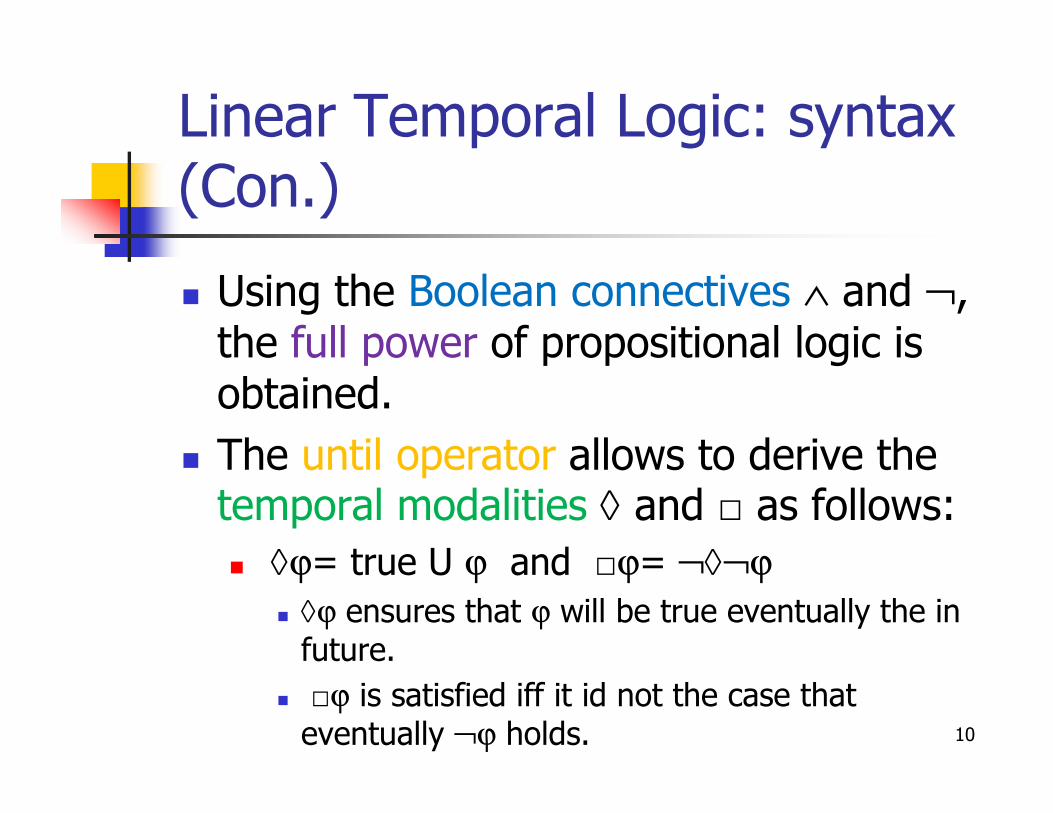
� Using the Boolean connectives ∧ and ¬, the full power of propositional logic is obtained.obtained.
� The until operator allows to derive the temporal modalities ◊ and □ as follows:
� ◊ϕ= true U ϕ and □ϕ= ¬◊¬ϕ
� ◊ϕ ensures that ϕ will be true eventually the in future.
� □ϕ is satisfied iff it id not the case that eventually ¬ϕ holds. 10

Linear Temporal Logic: syntax (Con.)
� The intuitive meaning of temporal modalities are illustrated below:
11

Linear Temporal Logic: syntax (Con.)
� By combining □ and ◊, new temporal modalities are obtained:
� □◊a describes the property stating that at � □◊a describes the property stating that at any moment j there is a moment i≥j at which a-state is visited. Thus a-state is visited infinitely often.
� ◊□a expresses that from moment j, only a-state are visited. Thus a-state is visited eventually forever.
12

Linear Temporal Logic: syntax (Con.)
� Example 5.2: properties for mutual exclusion problem:
� Safety property stating that P1 and P2� Safety property stating that P1 and P2
never simultaneously have access to their critical section: □(¬crit1∨¬crit2).
� Liveness property stating each process Pi is infinitely often in its critical section: (□◊crit1)∧ (□◊crit2).
� Read examples 5.3 and 5.4.13

Linear Temporal Logic: syntax (Con.)
� Let |ϕ| denote the length of LTL formula ϕ in terms of the number of operators in ϕ.operators in ϕ.
� This can be easily defined by inductionon the structure of:
� a∈AP has length 0;
� a∨b has length 2 and (a)U(a∧¬b) has
length 4.
14

Linear Temporal Logic: semantics
� LTL formula stands for properties of paths.
� The semantics of LTL formula is defined � The semantics of LTL formula is defined by a LT property. Then it is extended to an interpretation over paths and statesof a LTS.
15
Linear Temporal Logic: semantics (Con.)
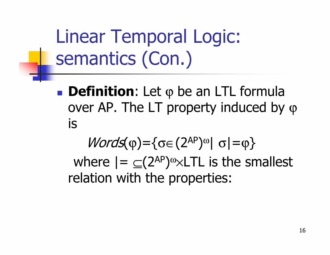
� Definition: Let ϕ be an LTL formula over AP. The LT property induced by ϕis is
Words(ϕ)={σ∈(2AP)ω| σ|=ϕ}
where |= ⊆(2AP)ω×LTL is the smallest relation with the properties:
16

Linear Temporal Logic: semantics (Con.)
� For the derived operators and the expected result is :
� Derive semantics of ◊□ and □◊!17

Linear Temporal Logic: semantics (Con.)
� Definition 5.7: Let TS=(S,Act,→,I,AP,L ) be a transition system without terminal state, and let ϕ be a LTL formula over AP.state, and let ϕ be a LTL formula over AP.
� For infinite path fragments π of TS, the satisfaction relation is defined by
π |= ϕ iff trace(π) |=ϕ
18
Linear Temporal Logic: semantics (Con.)
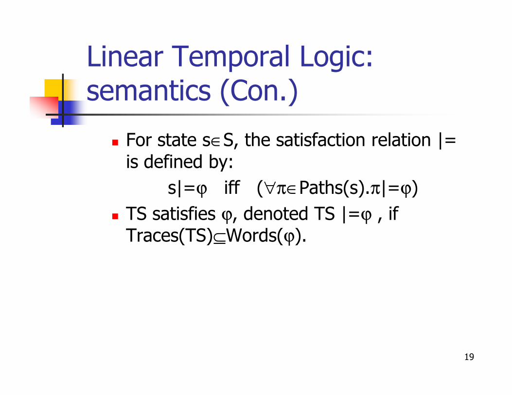
� For state s∈S, the satisfaction relation |= is defined by:
s|=ϕ iff (∀π∈Paths(s).π|=ϕ)ϕ ∀π∈ π ϕ
� TS satisfies ϕ, denoted TS |=ϕ , if Traces(TS)⊆Words(ϕ).
19

Linear Temporal Logic: semantics (Con.)
� From this definition, it immediately follows that:
� Thus, TS |=ϕ iff s0 |= ϕ for all initial states s0 of TS.
20
Linear Temporal Logic: semantics (Con.)
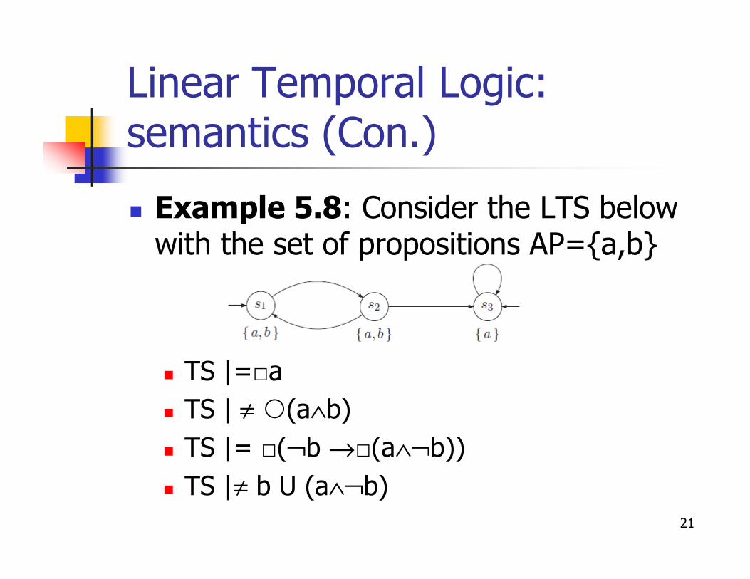
� Example 5.8: Consider the LTS below with the set of propositions AP={a,b}
� TS |=□a
� TS | ≠ (a∧b)
� TS |= □(¬b →□(a∧¬b))
� TS |≠ b U (a∧¬b)
21

Linear Temporal Logic: semantics (Con.)
� Semantics of Negation:
� For paths, it holds π|=ϕ iff π|≠¬ϕ. Since Words(¬ϕ)=(2AP)ω\Words(ϕ).Words(¬ϕ)=(2 ) \Words(ϕ).
� However statements TS|≠ϕ and TS|=¬ϕare not equivalent. Instead TS|=¬ ϕimplies TS|≠ϕ. Note that :
22
Linear Temporal Logic: semantics (Con.)
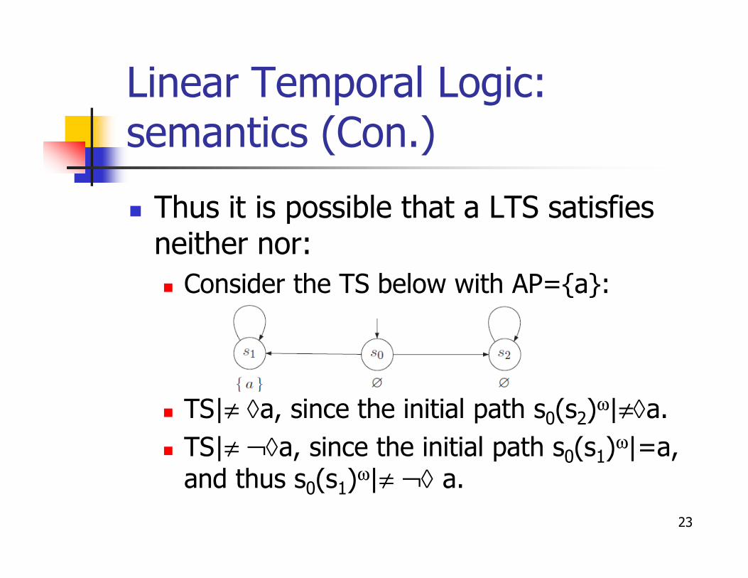
� Thus it is possible that a LTS satisfies neither nor:
� Consider the TS below with AP={a}:� Consider the TS below with AP={a}:
� TS|≠ ◊a, since the initial path s0(s2)ω|≠◊a.
� TS|≠ ¬◊a, since the initial path s0(s1)ω|=a,
and thus s0(s1)ω|≠ ¬◊ a.
23
Linear Temporal Logic: specifying properties
� Example 5.11: A modulo 4 counter can be represented by a sequential circuit C, which outputs 1 every fourth circuit C, which outputs 1 every fourth cycle, otherwise 0.
� Let the evaluation of r1r2 denote i=2.r1+r2
� C is constructed such that the output bit y is set exactly for i=0 (hence r1=0,r2=0). So
� δr1=r1⊕r2, δr2=¬r1, λy=¬r1∧¬r2.
24

Linear Temporal Logic: specifying properties (Con.)
� The circuit C and its transition system TSC
is shown below:
25

Linear Temporal Logic: specifying properties (Con.)
� Let AP={r1,r2,y}. The following statement holds:
� TSC |= □(y↔ ¬r1∧r2)
TSC |= (r → ( y ∨ y))� TSC |= □(r1→ (y ∨y))
� TSC |= □(y →(¬y ∧¬y)).
� The property that at least during every four cycles the output 1 id obtained holds for TSC:
� TSC |= □(y ∨y∨y∨y).
26
Linear Temporal Logic: specifying properties (Con.)
� The fact that these outputs are produced in a periodic manner where every fourth cycle yields the output 1 is expressed as:
TSC |= (y→( ¬y ∨ ¬y ∨ ¬y)).� TSC |= □(y→(¬y ∨ ¬y ∨¬y)).
� Read example 5.12
27
Linear Temporal Logic: specifying properties (Con.)
� Example 5.13: Leader election protocol:
� Goal: a process with a higher identifier is elected.elected.
� Processes are initially inactive, and may become active and then participate in the election (fairness: each process becomes active at some time).
� If an inactive process with higher id becomes active, a new leader election takes place.
28

Linear Temporal Logic: specifying properties (Con.)
� We use LTS to specify some properties. Let AP={leaderi,activei|1≤i,j≤N}.
� There is always one leader:� There is always one leader:
� □(\/1≤i≤N leaderi ∧ /\ 1≤j≤N,j≠i ¬leaderj)
� Since initially no leader exists we modify it to: □◊(\/1≤i≤N leaderi ∧ /\ 1≤j≤N,j≠i ¬leaderj)
� But this allows there to be more than one leader at a time temporarily, so:
(□ /\1≤i≤N(leaderi → /\ 1≤j≤N,j≠i ¬leaderj)) ∧(□◊(\/1≤i≤N leaderi )
29

Linear Temporal Logic: specifying properties (Con.)
� In the presence of an active process with a higher identity, the leader will resign at some time:
/\ 1≤i,j≤N,i<j ((leaderi ∧¬leaderj ∧activej)→◊¬
leaderi)
� A new leader will be an improvement over the previous one:
□¬ (/\ 1≤i,j≤N,i ≥j (leaderi ∧¬leaderi ∧ ◊leaderj))
� Read Example 5.14.30

Linear Temporal Logic: specifying properties (Con.)
� For synchronous systems LTL can be used as a formalism to specify real-time properties:properties:
� ϕ states that “at the next time instant ϕ
holds”.
� Kϕ =.. : ϕ holds after k time
instants.
� ◊≤k ϕ= \/0≤i≤kiϕ : ϕ will hold at most k
time instants.31

Linear Temporal Logic: specifying properties (Con.)
� □≤k ϕ= ¬\/0≤i≤ki¬ϕ : ϕ holds now and will
hold during the next k time instants.
� But for asynchronous systems the next-� But for asynchronous systems the next-step operator should be used with care.
32
Linear Temporal Logic: equivalence of LTL formulae
� Two formulae are intuitively equivalent whenever they have the same truth-value under all interpretations.value under all interpretations.
� Definition: LTL formulae ϕ1,ϕ2 are equivalent, denoted ϕ1≡ϕ2, if Words(ϕ1)=Words(ϕ2).
33
Linear Temporal Logic: equivalence of LTL formulae (Con.)
� As LTL subsumes propositional logic, equivalences of propositional logic also hold for LTL.hold for LTL.
� For temporal modalities we have:
34
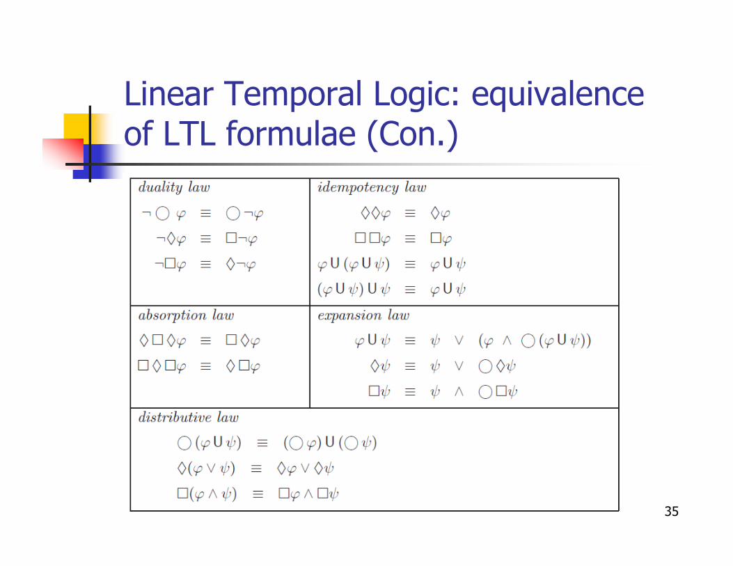
Linear Temporal Logic: equivalence of LTL formulae (Con.)
35
Linear Temporal Logic: equivalence of LTL formulae (Con.)
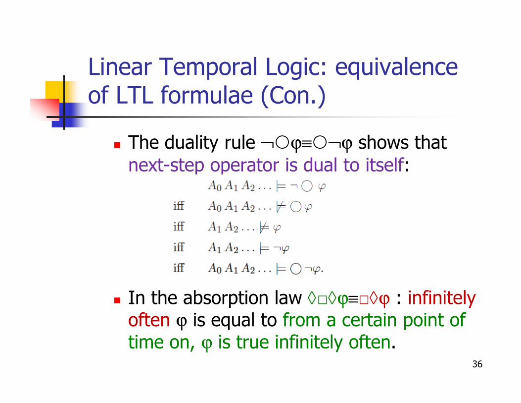
� The duality rule ¬ϕ≡¬ϕ shows that
next-step operator is dual to itself:
� In the absorption law ◊□◊ϕ≡□◊ϕ : infinitely often ϕ is equal to from a certain point of time on, ϕ is true infinitely often.
36

Linear Temporal Logic: equivalence of LTL formulae (Con.)
� The distributive laws for and disjunction, or and conjunction are dual to each other:
� ◊(ϕ∨ψ) ≡◊ϕ ∨ ◊ψ and □(ϕ∧ψ) ≡□ϕ ∧ □ψ
Recall that ∃(ϕ∨ψ) ≡ ∃ϕ ∨ ∃ψ and ∀(ϕ∧ψ) ≡� Recall that ∃(ϕ∨ψ) ≡ ∃ϕ ∨ ∃ψ and ∀(ϕ∧ψ) ≡∀ϕ ∧ ∀ψ
� But ◊(a∧b) ◊a ∧ ◊b and □(a∨b) □a ∨ □b (the same holds for ∃ and ∀):
37
≡ ≡
Linear Temporal Logic: equivalence of LTL formulae (Con.)
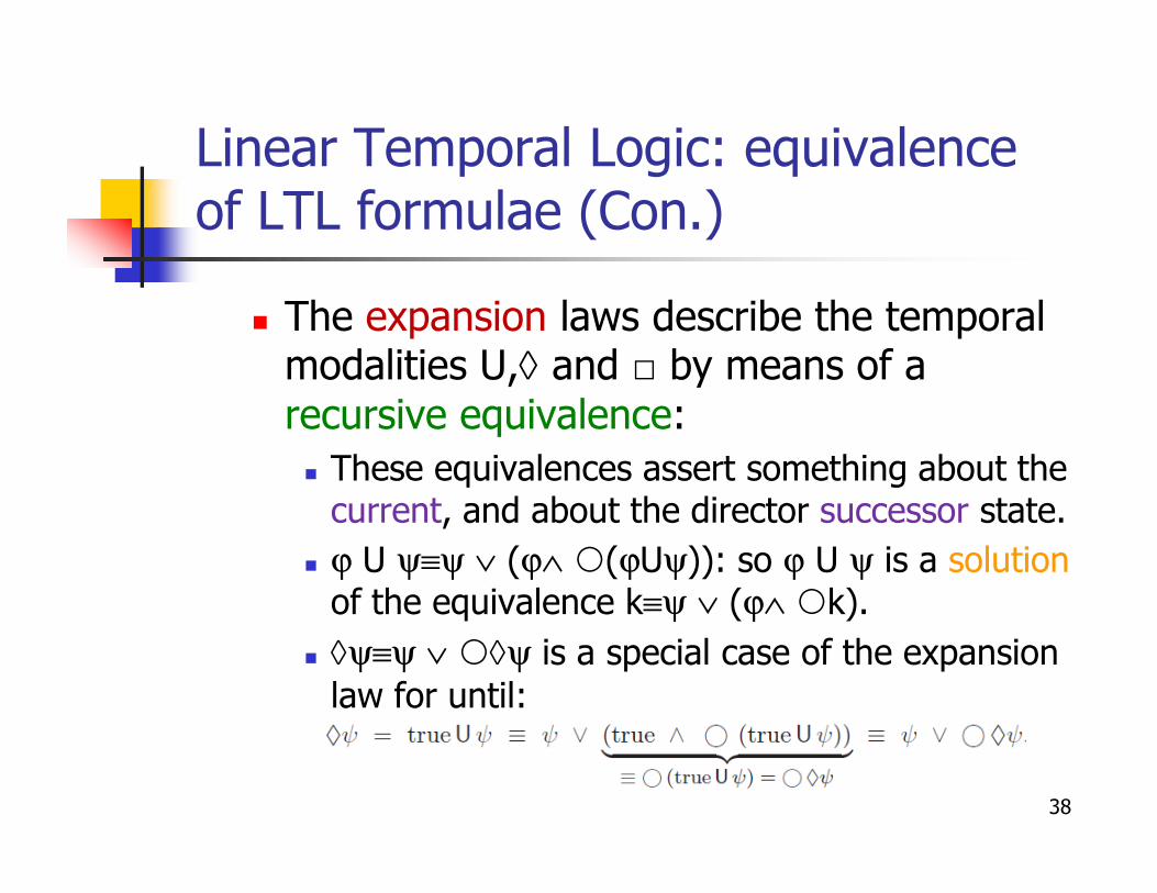
� The expansion laws describe the temporal modalities U,◊ and □ by means of a recursive equivalence:
These equivalences assert something about the � These equivalences assert something about the current, and about the director successor state.
� ϕ U ψ≡ψ ∨ (ϕ∧ (ϕUψ)): so ϕ U ψ is a solutionof the equivalence k≡ψ ∨ (ϕ∧ k).
� ◊ψ≡ψ ∨ ◊ψ is a special case of the expansion
law for until:
38

Linear Temporal Logic: equivalence of LTL formulae (Con.)
� Lemma 5.18 (Until is least solution of the expansion law): For LTL formulae ϕand ψ, Words(ϕUψ) is the least LT and ψ, Words(ϕUψ) is the least LT property P⊆(2AP)ω such that:
� Words(ψ) ∪{A0,A1,A2…∈Words(ϕ)|A1
A2…∈P}⊆P (I)
� Moreover, Words(ϕUψ) agrees with the set: Words(ψ) ∪{A0,A1,A2…∈Words(ϕ)|A1
A2…∈Words(ϕUψ)}.39
Linear Temporal Logic: equivalence of LTL formulae (Con.)
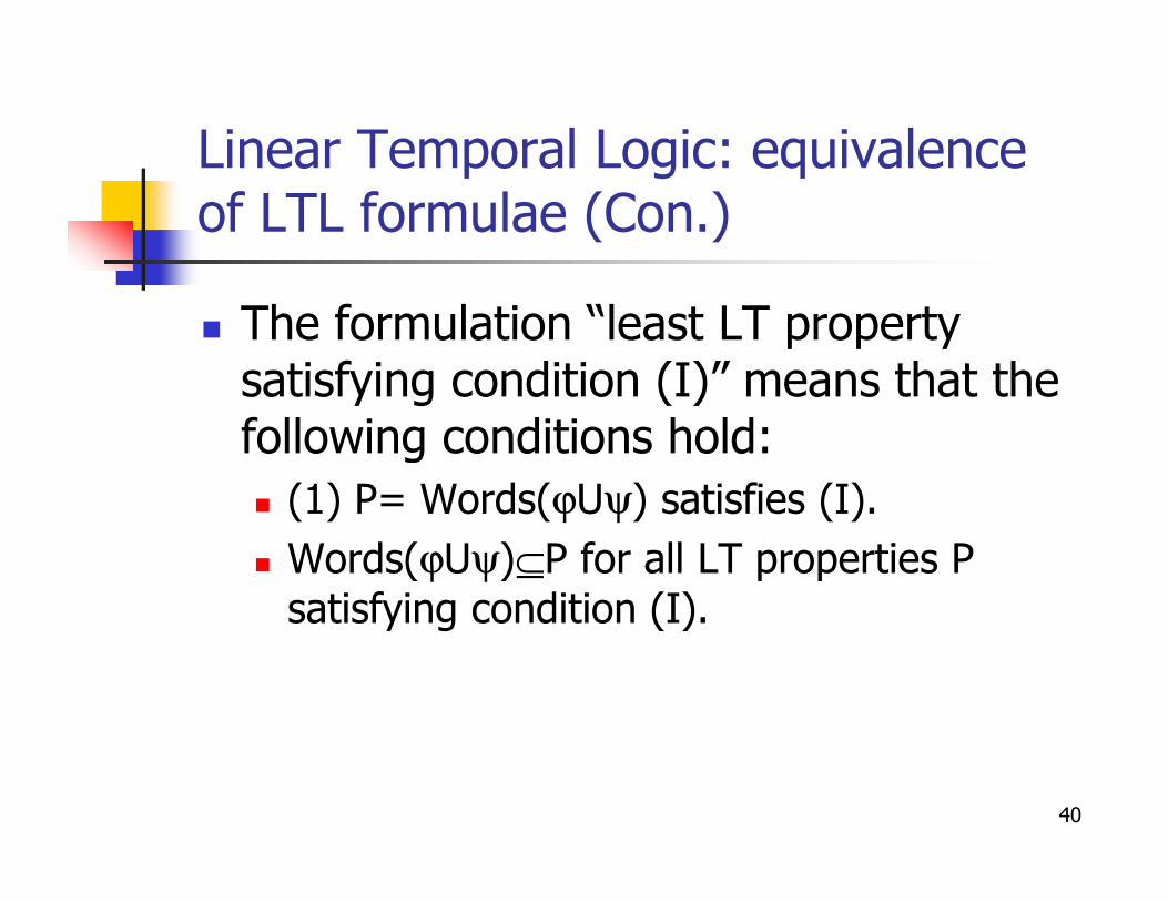
� The formulation “least LT property satisfying condition (I)” means that the following conditions hold:following conditions hold:
� (1) P= Words(ϕUψ) satisfies (I).
� Words(ϕUψ)⊆P for all LT properties P satisfying condition (I).
40

Linear Temporal Logic: weak, release and positive normal form
� Any LTL formula can be transformedinto a canonical form, called positive normal form (PNF), in which:normal form (PNF), in which:
� Negations only occur adjacent to atomic propositions.
� Recall that PNF formulae in propositional logic are constructed from true, false, the literals a and ¬a, and the operators ∧ and ∨.
41
Linear Temporal Logic: weak, release and positive normal form (Con.)
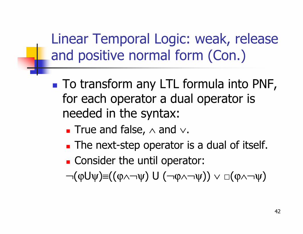
� To transform any LTL formula into PNF, for each operator a dual operator is needed in the syntax:needed in the syntax:
� True and false, ∧ and ∨.
� The next-step operator is a dual of itself.
� Consider the until operator:
¬(ϕUψ)≡((ϕ∧¬ψ) U (¬ϕ∧¬ψ)) ∨ □(ϕ∧¬ψ)
42

Linear Temporal Logic: weak, release and positive normal form (Con.)
� The operator W, called weak until or unless, as the dual of U: ϕWψ≡(ϕUψ) ∨□ϕ.
Until and W are dual in the following � Until and W are dual in the following sense:
� Note that W has the same expresivness to U.
� W and U satisfy the same expansion law.
43
Linear Temporal Logic: weak, release and positive normal form (Con.)
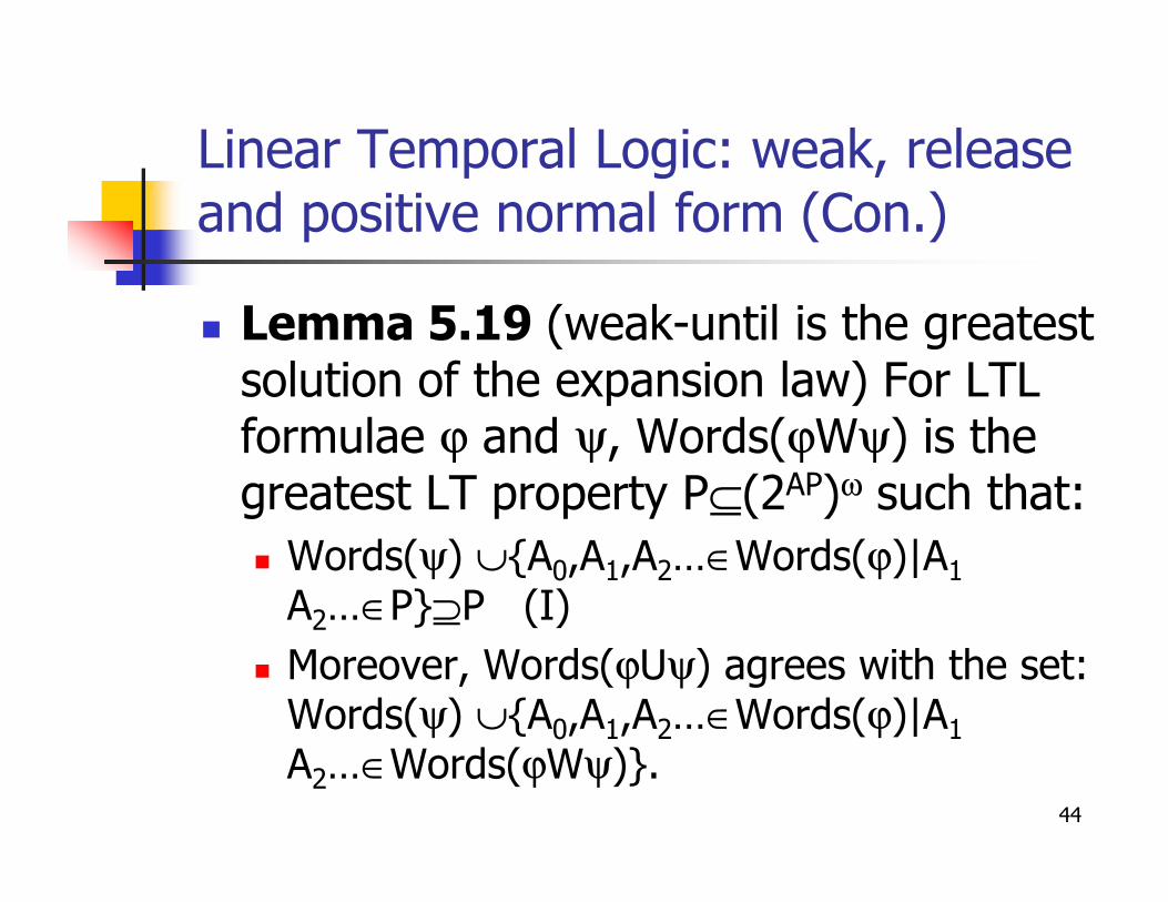
� Lemma 5.19 (weak-until is the greatest solution of the expansion law) For LTL formulae ϕ and ψ, Words(ϕWψ) is the formulae ϕ and ψ, Words(ϕWψ) is the greatest LT property P⊆(2AP)ω such that:
� Words(ψ) ∪{A0,A1,A2…∈Words(ϕ)|A1
A2…∈P}⊇P (I)
� Moreover, Words(ϕUψ) agrees with the set: Words(ψ) ∪{A0,A1,A2…∈Words(ϕ)|A1
A2…∈Words(ϕWψ)}.44

Linear Temporal Logic: weak, release and positive normal form (Con.)
� The formulation “greatest LT property satisfying condition (I)” means that the following conditions hold:following conditions hold:
� (1) P ⊇ Words(ϕWψ) satisfies (I).
� Words(ϕWψ) ⊇ P for all LT properties P satisfying condition (I).
45

Linear Temporal Logic: weak, release and positive normal form (Con.)
� Definition: For a∈AP, the set of LTL formulae in weak-until positive normal form (weak-until PNF) is given by:form (weak-until PNF) is given by:
� ϕ::= true | false | a | ¬a | ϕ1∧ψ2 | ϕ1∨ψ2 | ϕ | ϕ1Uψ2 | ϕ1Wψ2
� Since □ϕ≡ϕ W false and ◊ϕ≡true U ϕ, □and ◊ can be also considered as permitted operator of W-PNF.
46

Linear Temporal Logic: weak, release and positive normal form (Con.)
� We can convert each LTL formula to its W-PNF by using the following rewriterules:rules:
47
Linear Temporal Logic: weak, release and positive normal form (Con.)
� Example 5.21: convert LTL formula ¬□((aUb)∨ c) to weak-until PNF:
� ¬□((aUb)∨ c) � ¬□((aUb)∨ c)
≡ ◊¬((aUb)∨ c)
≡ ◊ (¬(aUb)∧ ¬c)
≡ ◊ ( (a∧ ¬ b) W (¬a ∧¬b) ∧ ¬c)
48

Linear Temporal Logic: weak, release and positive normal form (Con.)
� Theorem 5.22: For each LTL formula there exists an equivalent LTL formula in weak-until PNF.in weak-until PNF.
� The main draw-back of rewrite rules is that the length of the resulting formula may be exponential in the length of the original nonPNF LTL formula:
� The rewrite rule for U and W , duplicatesthe operands.
49
Linear Temporal Logic: weak, release and positive normal form (Con.)
� We can avoid this exponential blow-up by using another temporal modality as the dual of until, called release and the dual of until, called release and defined by :
� ϕRψ = ¬(¬ϕ U¬ψ)
� ϕRψ holds for a word if ψ always holds, a requirement that is released as soon as ϕbecomes valid.
50

Linear Temporal Logic: weak, release and positive normal form (Con.)
� The always operator is obtained from the release operator : □ϕ≡false R ϕ.
� The weak-until and the until operator � The weak-until and the until operator are obtained by:
� ϕWψ≡ (¬ϕ ∨ ψ) R (ϕ ∨ ψ) and vice versa ϕRψ≡ (¬ϕ ∧ ψ) W (ϕ ∧ ψ)
� ϕUψ≡ ¬(¬ϕ R ¬ψ)
51
Linear Temporal Logic: weak, release and positive normal form (Con.)
� Definition: For a∈AP, the set of LTL formulae in release positive normal form (release PNF) is given by:form (release PNF) is given by:
� ϕ::= true | false | a | ¬a | ϕ1∧ψ2 | ϕ1∨ψ2 | ϕ | ϕ1Uψ2 | ϕ1Rψ2
� Thus the rewrite rules are:
52

Linear Temporal Logic: weak, release and positive normal form (Con.)
� Theorem 5.24: For any LTL formula ϕthere exists an equivalent LTL formula ϕ’ in release PNF with |ϕ’|=O(|ϕ|).ϕ’ in release PNF with |ϕ’|=O(|ϕ|).
53
Linear Temporal Logic: Fairness in LTL
� Definition: Let Φ and Ψ be propositional logic formula over AP.
1. An unconditional LTL fairness constraint is an LTL formula of the form ufair=□◊Ψ.an LTL formula of the form ufair=□◊Ψ.
2. A strong LTL fairness condition is an LTL formula of the form ufair=□◊Φ→□◊Ψ.
3. A weak LTL fairness constraint is an LTL formula of the form wfair= ◊□Φ→□◊Ψ.
an LTL fairness assumption is a conjunction of LTL fairness constraints. 54

Linear Temporal Logic: Fairness in LTL (Con.)
� For instance, a strong LTL fairness assumption denote a conjunction of strong LTL fairness constraints:strong LTL fairness constraints:
sfair = /\0<i≤k(□◊Φi→□◊Ψi)
for propositional logic formulae Φi and Ψi over AP.
� Generally LTL fairness assumptions are: fair = ufair∧sfair ∧ wfair
55

Linear Temporal Logic: Fairness in LTL (Con.)
� Let FairPaths(s) denote the set of all fair paths starting in s and FairTraces(s) the set of all traces induced by fair the set of all traces induced by fair paths starting in s:
� FairPaths(s) ={π∈Paths(s) | π|=fair}
� FairTraces(s) = {Trace(π)|π∈FairPaths(s)}
� Above definitions can be lifted to TSs yielding FairPaths(TS) and FairTraces(TS).
56

Linear Temporal Logic: Fairness in LTL (Con.)
� Definition: For state s in TS (over AP) without terminal state, LTL formula ϕand LTL fairness assumptions fair letand LTL fairness assumptions fair let
� s |=fair ϕ iff ∀π∈FairPaths(s). π|= ϕ and
� TS|=fair ϕ iff s0∈I.s0|=fair ϕ.
� TS satisfies ϕ under the LTL fairness assumption fair if ϕ holds for all fair paths that originate from some initial state.
57

Linear Temporal Logic: Fairness in LTL (Con.)
� Example 5.27: Consider the mutual exclusion with randomized arbiter:
58

Linear Temporal Logic: Fairness in LTL (Con.)
� Arbiter tosses a coin, modeled by non-deterministic choice between heads and tails, to choose a process to enters its tails, to choose a process to enters its critical section.
� “process Pi is in its critical section infinitely often”:
� TS1 || Arbiter || TS2 |≠ crit1 (why?)
� TS1 || Arbiter || TS2 |=fair □◊crit1 ∧ □◊crit2where fair= □◊heads ∧ □◊tails.
59
Linear Temporal Logic: Fairness in LTL (Con.)
� In chapter 3, fairness was introduced using set of actions:
� An execution is unconditionally A-fair for a � An execution is unconditionally A-fair for a set of actions A, whenever each action α∈A occurs infinitely often.
� However LTL-fairness is defined on atomic propositions, i.e., from a state-based perspective.
60
Linear Temporal Logic: Fairness in LTL (Con.)
� Action-based fairness assumptions can always be translated into analogous LTL fairness assumption.fairness assumption.
� The intuition is
� Make a copy of each non-initial state s such that it is recorded which action was executed to enter s.
� The copied state <s,α> indicates that state s has been reached by performing α as last action. 61
Linear Temporal Logic: Fairness in LTL (Con.)
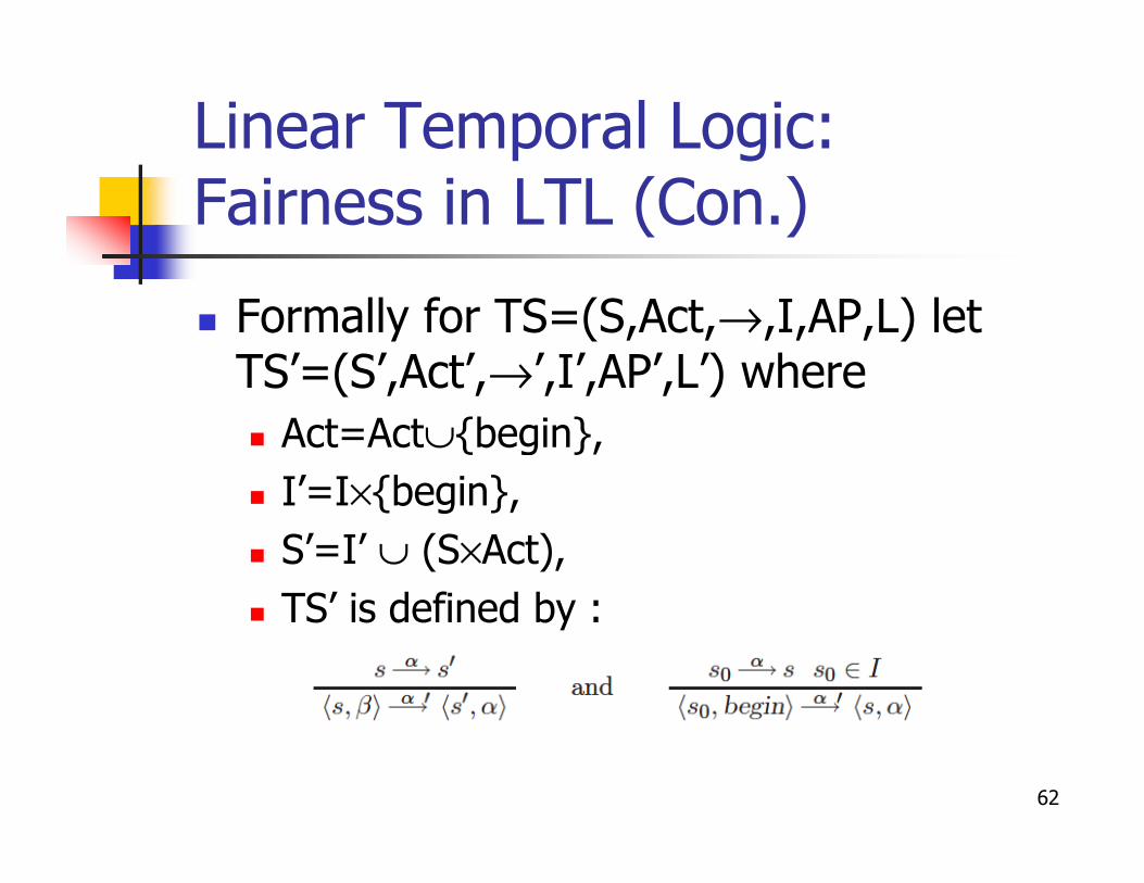
� Formally for TS=(S,Act,→,I,AP,L) let TS’=(S’,Act’,→’,I’,AP’,L’) where
� Act=Act∪{begin},� Act=Act∪{begin},
� I’=I×{begin},
� S’=I’ ∪ (S×Act),
� TS’ is defined by :
62

Linear Temporal Logic: Fairness in LTL (Con.)
� L’ is defined:
� L’(<s,α>)=L(s)∪{taken(α)}∪{enabled(β)|β∈Act(s)}
� L’(<s0,begin>)=L(s0)∪{enabled(β)|β∈Act(s0)}.
It can be established that� It can be established that
� TracesAP(TS)=TracesAP(TS’).
� Thus strong fairness for A⊆Act can be described by LTL fairness assumption:
� sfairA=□◊enabled(A)→ □◊taken(A)
� enabled(A)=\/α∈Aenabled(α), taken(A)=\/α∈Ataken(α)63
Linear Temporal Logic: Fairness in LTL (Con.)
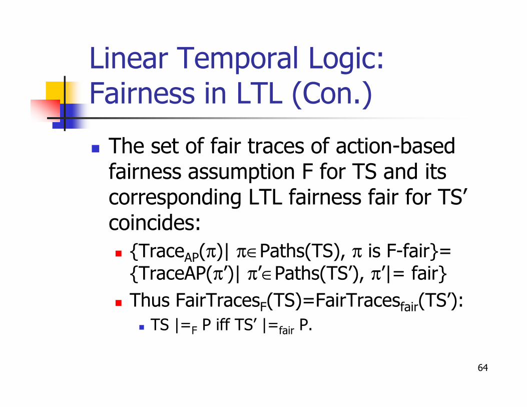
� The set of fair traces of action-based fairness assumption F for TS and its corresponding LTL fairness fair for TS’ corresponding LTL fairness fair for TS’ coincides:
� {TraceAP(π)| π∈Paths(TS), π is F-fair}= {TraceAP(π’)| π’∈Paths(TS’), π’|= fair}
� Thus FairTracesF(TS)=FairTracesfair(TS’):
� TS |=F P iff TS’ |=fair P.
64

Linear Temporal Logic: Fairness in LTL (Con.)
� Conversely, a (state-based) LTL fairness assumptions cannot always be represented as action-based fairness represented as action-based fairness assumption.
� Because strong or weak LTL fairness assumptions need not be realizable while action-based can be realized by a scheduler.
� State-based LTL fairness assumptions are more general then action-based. 65

Linear Temporal Logic: Fairness in LTL (Con.)
� Theorem 5:30: For transition system TS without terminal state, LTL formula ϕ, and LTL fairness assumption fair:ϕ, and LTL fairness assumption fair:
� TS|=fairϕ iff TS|=(fair→ϕ)
� Read Examples 5.28-30.
66

Automata-Based LTL Model Checking
� Given a finite transition system TS and an LTL formula ϕ (a requirement on TS), an LTL model-checking algorithm TS), an LTL model-checking algorithm checks TS |= ϕ:
� If ϕ is refuted, an error trace needs to be returned.
67

Automata-Based LTL Model Checking (Con.)
� In following, we assume that TS is finiteand has no terminal state.
� The model-checking algorithm that we � The model-checking algorithm that we are going to introduce is based on automata-based approach:
� Each LTL formula ϕ is represented by a nondeterministic büchi automaton (NBA).
� The basic idea is to disprove TS |= ϕ by looking for a path π in TS with π|= ¬ϕ .
68

Automata-Based LTL Model Checking (Con.)
� If such a path is found, a prefix of π is returned as error trace.
� If no such path is encountered, it is concluded that TS|=ϕ.concluded that TS|=ϕ.
� This Algorithm relies on following observation:
69

Automata-Based LTL Model Checking (Con.)
� Hence, for NBA A with Lω(A)=Words(¬ϕ) we have :
� TS |= ϕ if and only if Traces(TS)∩Lω(A)=∅.� TS |= ϕ if and only if Traces(TS)∩Lω(A)=∅.
� Thus, to check ϕ holds for TS, we first construct an NBA for the negation of the input formula ϕ and then look for their intersection TS⊗A¬ϕ.
70

Automata-Based LTL Model Checking (Con.)
� Definition: A nondeterministic Büchi automaton (NBA) A is a tuple A=(Q,Σ,δ,Q0,F) where:A=(Q,Σ,δ,Q0,F) where:
� Q is a finite set of states,
� Σ is an alphabet,
� δ:Q×Σ→2Q is a transition function,
� Q0⊆Q is a set of initial states, and
� F⊆Q is a set of accept (or:final) states, called the acceptance set.
71
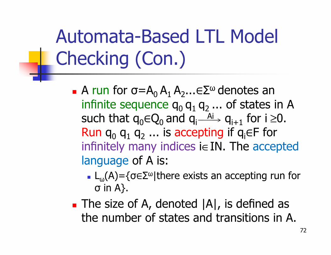
Automata-Based LTL Model Checking (Con.)
� A run for σ=A0 A1 A2...∈Σω denotes an infinite sequence q0 q1 q2 ... of states in A such that q0∈Q0 and qi
Ai qi+1 for i ≥0. Run q q q ... is accepting if q∈F for
∈
Run q0 q1 q2 ... is accepting if qi∈F for infinitely many indices i∈IN. The accepted language of A is:
� Lω(A)={σ∈Σω|there exists an accepting run for σ in A}.
� The size of A, denoted |A|, is defined as the number of states and transitions in A.
72

Automata-Based LTL Model Checking (Con.)
� Since the states Q of an NBA A is finite, each run for an infinite word σ∈Σω is infinite, and hence visits some state ∈
∈
infinite, and hence visits some state q∈Q infinitely often.
� Acceptance of a run depends on whether or not the set of all states that appear infinitely often in the given run contains an accept state.
� If F=∅, no run is accepting and Lω(A)=∅.73
Automata-Based LTL Model Checking (Con.)
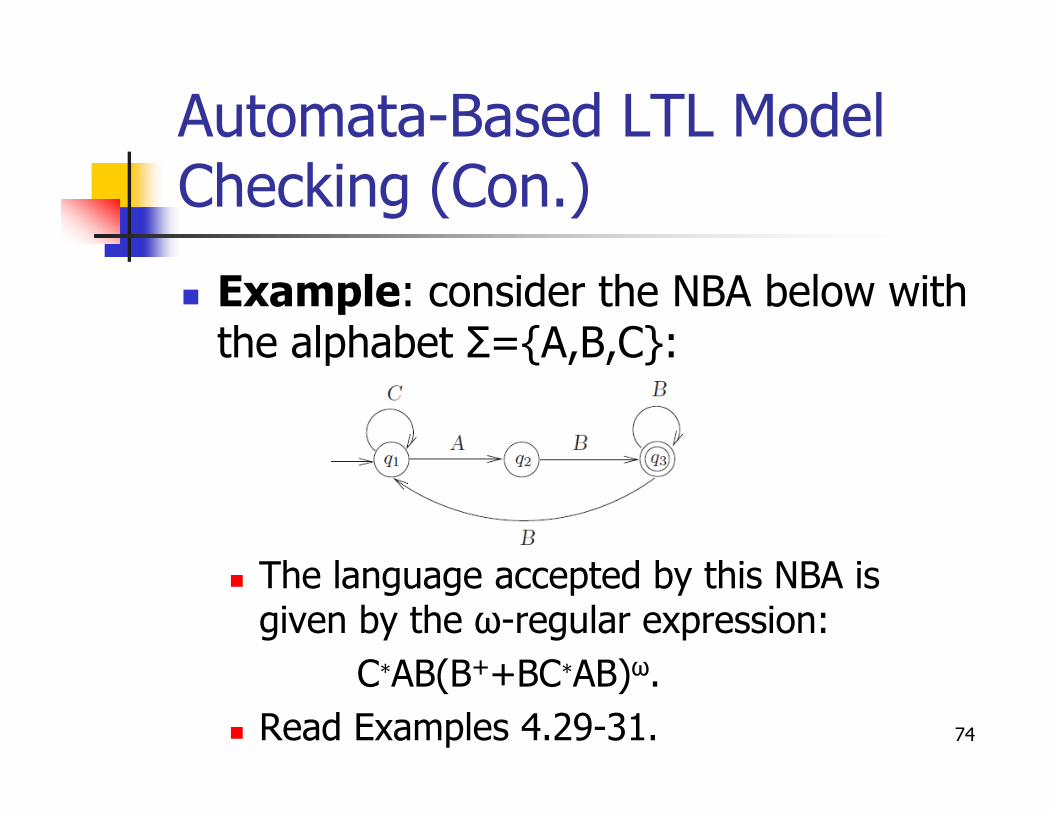
� Example: consider the NBA below with the alphabet Σ={A,B,C}:
� The language accepted by this NBA is given by the ω-regular expression:
C∗AB(B++BC∗AB)ω.
� Read Examples 4.29-31. 74

Criterion for the Nonemptiness of an NBA
� Lemma 4.41: Let A = (Q,Σ,δ,Q0,F) be an NBA.
Then the following two statements are equivalent:equivalent:� Lω(A)≠Ø,
� There exists a reachable accept q that belongs to a cycle in A. Formally
∃q0∈Q0 ∃q∈F ∃w∈Σ* ∃v∈Σ+ . q∈δ*(q0,w)∩δ*(q,v)
75

Checking Emptiness for NBA
�Theorem 4.42: The emptiness problem for NBA A can be solved in time O(|A|).
A
can be solved in time O(|A|).
76
Automata-Based LTL Model Checking (Con.)
� Definition: Let A=(Q,Σ,δ,Q0,F) be an NBA. A is called nonblocking if δ(q,A)≠∅for all states q and all symbols A∈Σ.
∈
∅
for all states q and all symbols A∈Σ.
� Note that for a given nonblocking NBA A and input word σ∈Σω, there is at least one (infinite) possibly non-accepting run for σin A.
� Thus it is not a restriction to assume a NBA is nonblocking .
77

Automata-Based LTL Model Checking (Con.)
� Definition: A persistence property over AP is an LT property Ppers⊆(2AP)ω
“eventually forever Φ” for some
∈ ∀
⊆
“eventually forever Φ” for some propositional logic formula Φ over AP:
� Ppers={A0A1A2...∈(2AP)ω|∀∞j.Aj|=Φ}
where ∀∞j is short for ∃i≥0.∀j≥i. Formula Φ is called a persistence (or state) condition of Ppers.
78

Automata-Based LTL Model Checking (Con.)
� Intuitively, a persistence property “eventually forever Φ” ensures the tenacity of the state property given by tenacity of the state property given by the persistence condition Φ.
� In other words Φ is an invariant after a while; i.e., from a certain point on all states satisfy Φ.
79

Automata-Based LTL Model Checking (Con.)
� The formula “eventually forever Φ” is true for a path if and only if almost all ,i.e., all except for finitely many, states ,i.e., all except for finitely many, states satisfy the proposition Φ.
� Our goal is to show that the question whether Traces(TS)∩Lω(A)=∅ holds can be reduced to the question whether a certain persistence property holds in the product of TS and A.
80

Automata-Based LTL Model Checking (Con.)
� Defintion: Let TS=(S,Act,→,I,AP,L) be a transition system without terminal states and A=(Q,2AP,δ,Q0,F) a non-blocking
⊗
and A=(Q,2 ,δ,Q0,F) a non-blockingNBA. Then, product TS and A is:
� TS⊗A=(S×Q,Act,→’,I’,AP’,L’) where →’ is the smallest relation defined by the rule:
81
L(t )s t q p
s,q t, p
α
α
→ ∧ →
′⟨ ⟩ → ⟨ ⟩
Automata-Based LTL Model Checking (Con.)
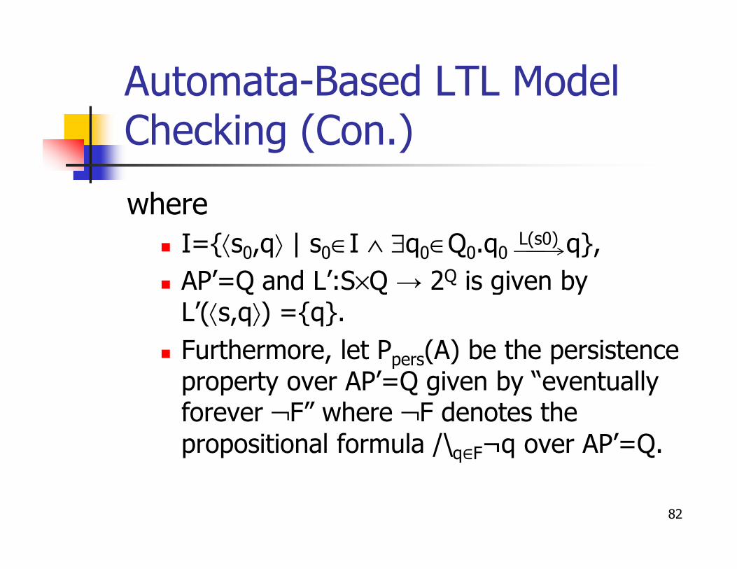
where
� I={⟨s0,q⟩ | s0∈I ∧ ∃q0∈Q0.q0 L(s0) q},
� AP’=Q and L’:S×Q → 2Q is given by � AP’=Q and L’:S×Q → 2Q is given by L’(⟨s,q⟩) ={q}.
� Furthermore, let Ppers(A) be the persistence property over AP’=Q given by “eventually forever ¬F” where ¬F denotes the propositional formula /\q∈F¬q over AP’=Q.
82
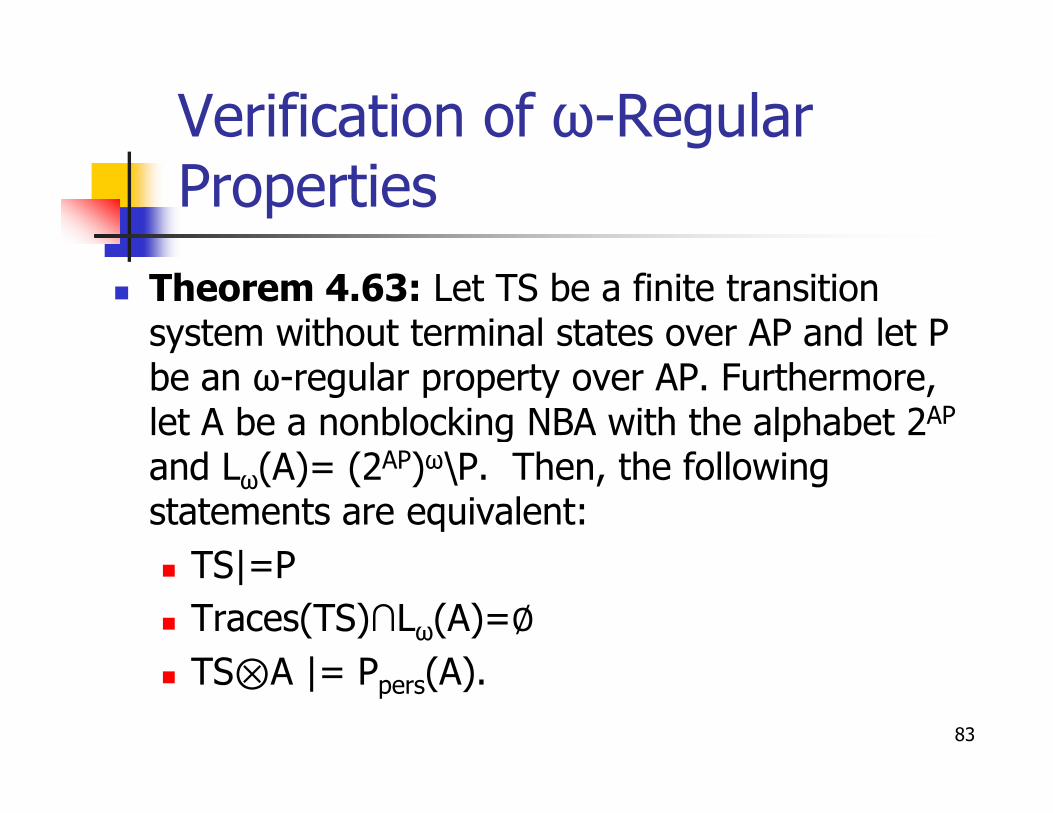
Verification of ω-Regular Properties
� Theorem 4.63: Let TS be a finite transition system without terminal states over AP and let P be an ω-regular property over AP. Furthermore, let A be a nonblocking NBA with the alphabet 2APlet A be a nonblocking NBA with the alphabet 2AP
and Lω(A)= (2AP)ω\P. Then, the following statements are equivalent:
� TS|=P
� Traces(TS)∩Lω(A)=∅
� TS⊗A |= Ppers(A).
83

Persistence Checking and Cycle Detection
� Theorem 4.65: Let TS be a finite transition system without terminal states over AP, Φ be a propositional formula over AP, and Ppers the persistence property “eventually forever Φ”. Then, persistence property “eventually forever Φ”. Then, the following statements are equivalent:
� TS |≠ Ppers
� There exists a reachable ¬Φ state s which belongs to a cycle. Formally:
∃s ∈ Reach(TS). s |≠ Φ ∧ s is on a cycle in G(TS).
84

Naïve Persistence Checking
85

Cycle Detection
86

Persistence Checking by nested depth-first search
87

Time Complexity of Persistence Checking
� Theorem 4.70: The worst-case time complexity of Algorithm 8 is O((N+M)+N.|Φ|)
where N is the number of reachable states, where N is the number of reachable states, and M the number of transitions between the reachable states.
88

Automata-Based LTL Model Checking (Con.)
� Thus the LTL model-checking algorithm is:
89

Automata-Based LTL Model Checking (Con.)
� Now it remains to show that how a given LTL property can be presented by a NBA and such an NBA can be a NBA and such an NBA can be constructed algorithmically.
� Recall that the LTL semantics yields a language Words(ϕ)⊆(2AP)ω. Thus the alphabet of NBA for LTL formulae is Σ=2AP.
� We show that Words(ϕ) is ω-regular, and hence, can be represented by a NBA.
90
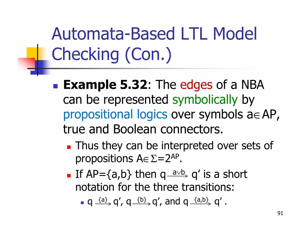
Automata-Based LTL Model Checking (Con.)
� Example 5.32: The edges of a NBA can be represented symbolically by propositional logics over symbols a∈AP, propositional logics over symbols a∈AP, true and Boolean connectors.
� Thus they can be interpreted over sets of propositions A∈Σ=2AP.
� If AP={a,b} then q a∨b q’ is a short notation for the three transitions:
� q {a} q’, q {b} q’, and q {a,b} q’ .91

Automata-Based LTL Model Checking (Con.)
� The language of all words σ=A0A1…∈2AP
satisfying the LTL formula □◊green is accepted by the NBA below:
� A is in the accept state q1 if and only if the last consumed symbol (the last set Ai of the input word A0A1A2...∈(2AP)ω) contains the propositional symbol green.
92

Automata-Based LTL Model Checking (Con.)
� The liveness property: “whenever event a occurs, event b will eventually occur”. An associated NBA over the alphabet An associated NBA over the alphabet 2{a,b} is shown below:
93

Automata-Based LTL Model Checking (Con.)
� To construct an NBA A satisfying Lω(A)=Words(ϕ) for the LTL formula ϕ, first a generalized NBA is constructed first a generalized NBA is constructed for ϕ, which subsequently is transformed into an equivalent NBA.
94

Automata-Based LTL Model Checking (Con.)
� The whole picture of LTL model checking:
95
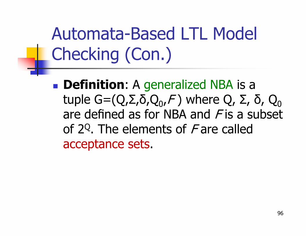
Automata-Based LTL Model Checking (Con.)
� Definition: A generalized NBA is a tuple G=(Q,Σ,δ,Q0,F ) where Q, Σ, δ, Q0
are defined as for NBA and F is a subset are defined as for NBA and F is a subset of 2Q. The elements of F are called acceptance sets.
96

Automata-Based LTL Model Checking (Con.)
� The accepted language Lω(G) consists of all infinite words in (2AP)ω that have at least one infinite run q0q1q2... in G
∈
at least one infinite run q0q1q2... in G such that for each acceptance set F∈Fthere are infinitely many indices i with qi∈F.
� A GNBA for which F is a singleton set can be regarded as an NBA.
97
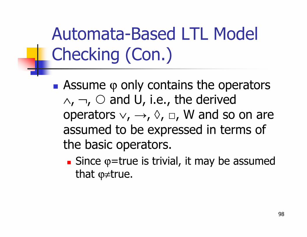
Automata-Based LTL Model Checking (Con.)
� Assume ϕ only contains the operators ∧, ¬, and U, i.e., the derived operators ∨, →, ◊, □, W and so on are operators ∨, →, ◊, □, W and so on are assumed to be expressed in terms of the basic operators.
� Since ϕ=true is trivial, it may be assumed that ϕ≠true.
98

Automata-Based LTL Model Checking (Con.)
� The basic idea to construct a GNBA over the alphabet 2AP for a given LTL formula ϕ (over AP), i.e., Lω(gϕ)=Words(ϕ) is:ϕ (over AP), i.e., Lω(gϕ)=Words(ϕ) is:
� Let σ=A0 A1 A2 …∈Words(ϕ).
� The sets Ai⊆AP are expanded by subformulae ψ (and their negation) of ϕsuch that an infinite word σ=B0 B1 B2 … with the following property arises:
� ψ∈Bi if and only if Ai Ai+1 Ai+2 …|=ψ
99σi

Automata-Based LTL Model Checking (Con.)
� The GNBA gϕ is constructed such that Bi
constitute its states.
� Moreover, the construction ensures that σ=B0
B B … is a run for σ= A A A … in G .σ 0
B1 B2 … is a run for σ= A0 A1 A2 … in Gϕ.
� The accepting conditions for gϕ are chosen such that the run σ is accepting if and only if σ|=ϕ.
� We encode the meaning of the logical operators into the states, transitions and acceptance sets of Gϕ. 100

Automata-Based LTL Model Checking (Con.)
� Let ϕ= aU(¬a∧b) and σ={a}{a,b}{b}…:
� Bi is a subset of the set of formulae {a,b,¬a,¬a∧b,ϕ}∪{¬b,¬(¬a∧b),¬ϕ).{a,b,¬a,¬a∧b,ϕ}∪{¬b,¬(¬a∧b),¬ϕ).
� The set A0={a} is extended with formulae ¬b, ¬(¬a∧b) and ϕ, since all these formula hold in σ0=σ and all other subformulae in the above set are refuted by σ.
� The set A1={a,b} is extended with the formulae ¬(¬a∧b) and ϕ, as they hold in σ1={a,b}{b}…. 101

Automata-Based LTL Model Checking (Con.)
� The A2={b} is extended with ¬a, ¬a∧b and ϕ as they hold in σ2={b}….
� These yield σ= {a,¬b,¬(¬a∧b),ϕ} {a,b,¬(¬a∧b),ϕ} {¬a,b,¬a∧b,ϕ}…
σ ¬ ¬ ¬ ∧ ϕ{a,b,¬(¬a∧b),ϕ} {¬a,b,¬a∧b,ϕ}…
102

Automata-Based LTL Model Checking (Con.)
� Definition: The closure of LTL formula ϕ is the set closure(ϕ) consisting of all subformulae ψ of ϕ and their negationsubformulae ψ of ϕ and their negation¬ψ (where ψ and ¬¬ψ are identical).
� For instance, for ϕ= aU(¬a∧b) , the closure(ϕ)={a,b,¬a,¬b, ¬a∧b,¬(¬a∧b),ϕ, ¬ϕ}.
� |closure(ϕ)|∈O(|ϕ|)
103
Automata-Based LTL Model Checking (Con.)
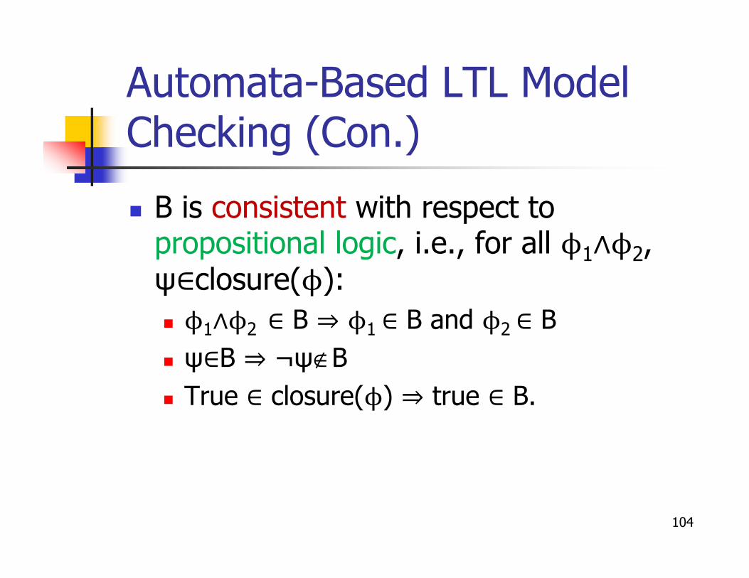
� B is consistent with respect to propositional logic, i.e., for all ϕ1∧ϕ2,ψ∈closure(ϕ):
ϕ ∧ϕ ∈ ⇒ ϕ ∈ ϕ ∈
∈ ⇒
ϕ ∧ϕ
ψ∈closure(ϕ):
� ϕ1∧ϕ2 ∈ B ⇒ ϕ1 ∈ B and ϕ2 ∈ B
� ψ∈B ⇒ ¬ψ∉B
� True ∈ closure(ϕ) ⇒ true ∈ B.
104

Automata-Based LTL Model Checking (Con.)
� B is locally consistent with respect to the until operator, i.e., for all ϕ1Uϕ2 ∈ closure(ϕ):
Φ ∈ B ⇒ ϕ Uϕ ∈ B
ϕ ϕ ∈ ϕ ⇒ ϕ ∈
ϕ ϕ ∈ ϕ
� Φ2 ∈ B ⇒ ϕ1Uϕ2 ∈ B
� ϕ1Uϕ2 ∈ B and ϕ2 ∉ B ⇒ ϕ1 ∈ B.
� B is maximal, i.e., for all ψ ∈ closure(ϕ):
� ψ∉B ⇒ ¬ψ∈B.
105
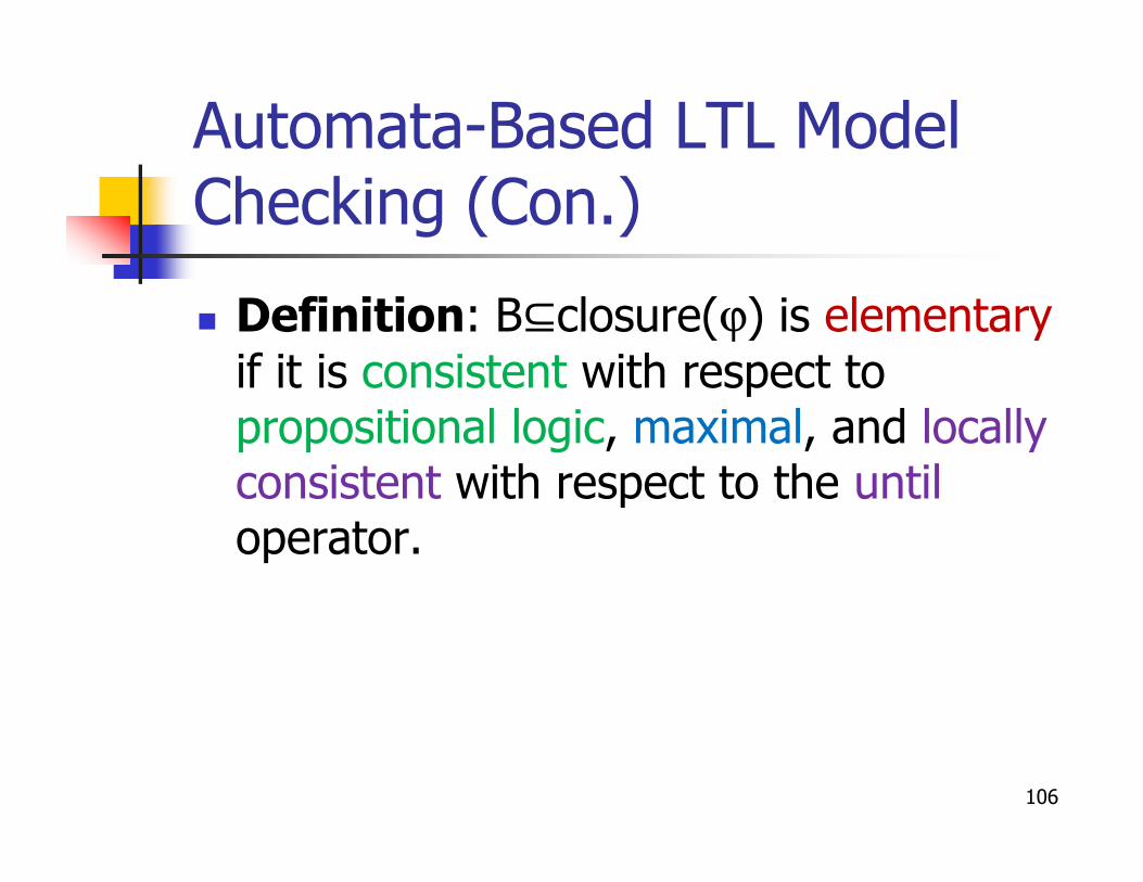
Automata-Based LTL Model Checking (Con.)
� Definition: B⊆closure(ϕ) is elementaryif it is consistent with respect to propositional logic, maximal, and locally
⊆
propositional logic, maximal, and locally consistent with respect to the untiloperator.
106

Automata-Based LTL Model Checking (Con.)
� Example 5.35: let ϕ=aU(¬a∧b):
� B0={a,b,ϕ} is consistent with respect to propositional logic and locally consistent propositional logic and locally consistent with respect to the until operator. But it is not maximal. Why?
� B1={a,b,¬a∧b,ϕ} is not consistent with respect to propositional logic. Why?
� B2={a,b, ¬(¬a∧b), ϕ} is an elementary set.
107
Automata-Based LTL Model Checking (Con.)
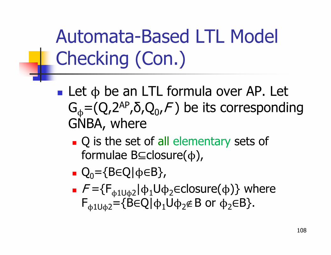
� Let ϕ be an LTL formula over AP. Let Gϕ=(Q,2AP,δ,Q0,F ) be its corresponding GNBA, where
⊆ ϕ
ϕ
ϕ
GNBA, where
� Q is the set of all elementary sets of formulae B⊆closure(ϕ),
� Q0={B∈Q|ϕ∈B},
� F ={Fϕ1Uϕ2|ϕ1Uϕ2∈closure(ϕ)} where Fϕ1Uϕ2={B∈Q|ϕ1Uϕ2∉B or ϕ2∈B}.
108
Automata-Based LTL Model Checking (Con.)
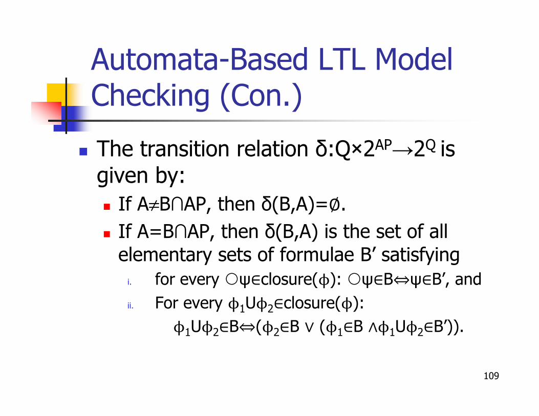
� The transition relation δ:Q×2AP→2Q is given by:
� If A≠B∩AP, then δ(B,A)=∅. � If A≠B∩AP, then δ(B,A)=∅.
� If A=B∩AP, then δ(B,A) is the set of all elementary sets of formulae B’ satisfying
i. for every ψ∈closure(ϕ): ψ∈B⇔ψ∈B’, and
ii. For every ϕ1Uϕ2∈closure(ϕ):
ϕ1Uϕ2∈B⇔(ϕ2∈B ∨ (ϕ1∈B ∧ϕ1Uϕ2∈B’)).
109

Automata-Based LTL Model Checking (Con.)
� The conditions (i) and (ii) reflect the semantics of the next step and the until operator, respectively. Rule (ii) is
ϕ ϕ ϕ ∨ ϕ ∧ ϕ ϕ
operator, respectively. Rule (ii) is justified by the expansion rule:
� ϕ1Uϕ2 ≡ ϕ2 ∨ (ϕ1∧ (ϕ1Uϕ2)).
110

Automata-Based LTL Model Checking (Con.)
� To model the semantics of U, an acceptance set Fψ is introduced for every subformula ψ=ϕ1Uϕ2 of ϕ.
∈
ϕ ∈ ϕ ∈
every subformula ψ=ϕ1Uϕ2 of ϕ.
� Thus every run B0 B1 B2 ... for which ψ∈B0, we have ϕ2∈Bj (for some j≥0) and ϕ1∈Bi
for all i<j.
� The requirement that a word σ satisfies ϕ1Uϕ2 only if ϕ2 will actually eventually become true is ensured by the accepting set Fϕ1Uϕ2. 111

Automata-Based LTL Model Checking (Con.)
� Example 5.38: let ϕ=a. It
corresponding GNBA Gϕ is:
� Q = {B1,B2,B3,B4} where B1={a,a}, � Q = {B1,B2,B3,B4} where B1={a,a}, B2={a,¬a}, B3={¬a,a}, B4={¬a,¬a},
� Q0={B1,B3} since a∈B1,B3,
� 2{a}={∅,{a}} and δ is defined:
� B1∩{a}={a}, so δ(B1,{a})={B1,B2} since a∈B1 and B1 and B2 are the only states that
contain a.
� B1∩∅=∅, so δ(B1,∅)=∅. 112

Automata-Based LTL Model Checking (Con.)
� The resulting GNBA is shown below:
� Read Example 5.39.113

Automata-Based LTL Model Checking (Con.)
� Any state of the GNBA for an LTL formula ϕ contains either ψ or its negation ¬ψ for every subformula ψ of ϕ
ffi
ϕ
negation ¬ψ for every subformula ψ of ϕ.
� This is somewhat redundant. It suffices to represent state B∈closure(ϕ) by the propositional symbols a∈B∩AP, and the formulae ψ or ϕ1Uϕ2∈B.
114
Automata-Based LTL Model Checking (Con.)
� Having constructed a GNBAG ϕ for a given LTL formula ϕ, an NBA for ϕ can be obtained by the transformation
ϕ
ϕ ϕ
be obtained by the transformation“GNBA�NBA” described in following.
115

Automata-Based LTL Model Checking (Con.)
� Let G=(Q,Σ,δ,Q0,F ) be a GNBA. Let F ={F1,...,Fk} where k≥1.
� The basic idea of the construction of A is to � The basic idea of the construction of A is to create k copies of G such that the acceptance set Fi of the ith copy is connected to the corresponding states of the (i+1)th copy.
116

Automata-Based LTL Model Checking (Con.)
� The accepting condition for A consists of the requirement that an accepting state of the first copy is visited infinitely often:
This ensures that all other accepting sets F of � This ensures that all other accepting sets Fi of the k copies are visited infinitely often too:
117

Automata-Based LTL Model Checking (Con.)
� Formally, let A=(Q’,Σ,δ’,Q0’,F’) be the corresponding NBA,where:
� Q’=Q×{1,...,k},� Q’=Q×{1,...,k},
� Q0’=Q0×{1}={⟨q0,1⟩|q0∈Q0},
� F’=F1×{1}={⟨qF,1⟩|qF∈F1},
� The transition function δ’ is given by
{⟨q’,i⟩|q’∈δ(q,A)} if q∉Fi
� δ'(⟨q,i⟩,A)= {⟨q’,i+1⟩|q’∈δ(q,A)} otherwise
� We identify ⟨q,1⟩ and ⟨q,k+1⟩. 118
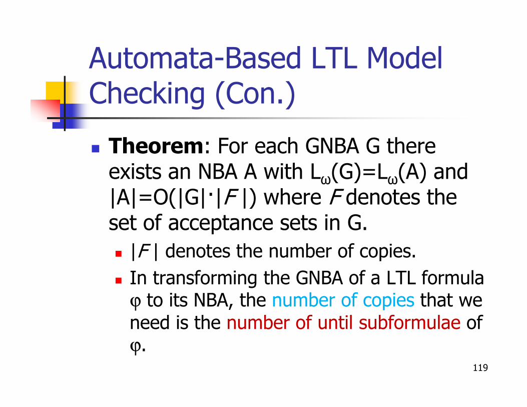
Automata-Based LTL Model Checking (Con.)
� Theorem: For each GNBA G there exists an NBA A with Lω(G)=Lω(A) and |A|=O(|G|�|F |) where F denotes the |A|=O(|G|�|F |) where F denotes the set of acceptance sets in G.
� |F | denotes the number of copies.
� In transforming the GNBA of a LTL formula ϕ to its NBA, the number of copies that we need is the number of until subformulae of ϕ.
119

Automata-Based LTL Model Checking (Con.)
� Theorem: For any LTL formula ϕ (over AP) there exists an NBA Aϕ with Words(ϕ)=Lω(Aϕ) which can be
ϕ
ϕ
ϕ
Words(ϕ)=Lω(Aϕ) which can be constructed in time and space 2O(|ϕ|).
� It should be noted that the size of the resulting GNBA grows up exponentiallywith respect to the size of formula.
120

Complexity of the LTL Model-checking problem
� As explained before, the essential idea behind the automata-based model-checking algorithm for LTL is based checking algorithm for LTL is based upon the following relations:
121

Complexity of the LTL Model-checking problem (Con.)
� The GNBA Gϕ has at most 2|ϕ| states with |ϕ| accepting states (the number of until-subformulas in ϕ).
The NBA A ϕ can thus be constructed in
ϕ
ϕ
� The NBA A¬ϕ can thus be constructed in exponential time: O(2|ϕ| ×|ϕ|)=O(2|ϕ|+log|ϕ|).
� Thus an upper bound for the time-and space-complexity of LTL model checking is O(|TS|×2|ϕ|).
122
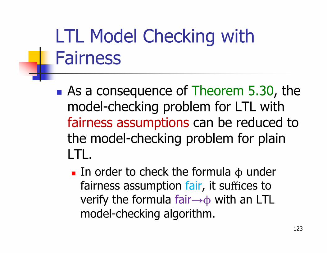
LTL Model Checking with Fairness
� As a consequence of Theorem 5.30, the model-checking problem for LTL with fairness assumptions can be reduced to fairness assumptions can be reduced to the model-checking problem for plain LTL.
� In order to check the formula ϕ under fairness assumption fair, it suffices to verify the formula fair→ϕ with an LTL model-checking algorithm.
123

LTL Model Checking with Fairness (Con.)
� The drawback of this approach is that the length |fair| can have an exponential influence on the run-time of exponential influence on the run-time of the algorithm.
� The construction of an NBA for the negated formula ¬(fair→ϕ) is exponential in |¬(fair→ϕ)|= |fair| + |ϕ|.
� To avoid this, a modified persistence check can be exploited to analyze TS⊗A¬ϕ
(instead of TS⊗A¬(fair→ϕ)). 124