chapter 6 understanding spatial and temporal processes of ......linear function of temporal land...

Chapter 6∗∗∗∗ Understanding Spatial and Temporal Processes of Urban Growth

Abstract Understanding the dynamic process of urban growth is a prerequisite to the prediction of land cover change and the support of urban development planning and sustainable growth management. The spatial and temporal complexity inherent in urban growth requires the development of a new simulation approach, which should be process-oriented and have stronger capacities for interpretation. This chapter presents an innovative methodology for understanding spatial processes and their temporal dynamics on two interrelated scales (municipality and project), by means of a multi-stage framework and a dynamic weighting concept. The multi-stage framework aims to model local spatial processes and global temporal dynamics by incorporating explicit decision-making processes. It is divided into four stages: project planning, site selection, local growth and temporal control. These four steps represent the interactions between the top-down and bottom-up decision-making involved in land development for large-scale projects. Project-based cellular automata modelling is developed for interpreting the spatial and temporal logic between various projects forming the whole urban growth. Dynamic weighting attempts to model local temporal dynamics at the project level as an extension of the local growth stage. As a non-linear function of temporal land development, dynamic weighting is able to link spatial processes and temporal patterns. The methodology is tested with reference to the urban growth of a fast growing city, Wuhan in the P.R.China from 1993 to 2000. The findings from this research suggest that this methodology can interpret and visualise the dynamic process of urban growth more temporally and transparently, globally and locally. Key words: urban growth, spatial and temporal processes, cellular automata, multi-stage, dynamic weighting.

∗ Based on (Cheng and Masser, 2002) and (Cheng and Masser, 2003b)

Chapter 6

136

6.1 Introduction Understanding the urban development processes is highly crucial in urban development planning and sustainable growth management. The urban development process involves multi-actors, multi-behaviours and various policies, which results in its spatial and temporal complexity. The non-linear dynamics inherent in these growth processes opens up the possibility for emergencies (sudden changes) that are difficult or impossible to predict. Due to the hidden complexity of reality, our science has become less orientated to prediction but more an aid to understanding and structuring debate (Batty and Torrens, 2001). Orjan (1999) argued that without a proper understanding of the recent past we are in no position to comprehend − let alone predict − emerging patterns and processes. Couclelis (1997) first put forward the idea of a spatial understanding support system (SUSS). Horita (2000) reported a new SUSS for representing community disputes. Limited by existing sciences and techniques, understanding-oriented modelling is oriented to more practicability than to prediction, or, rather, a proper understanding of the complex system is the prerequisite to its prediction. Towards reasonable understanding, we need reliable information sources and models. Successful models should have a strong capacity for interpretation and an interactive environment to simulate 'what-if' scenarios. Consequently, an innovative simulation approach is required. The first step to aid such decision-making is to identify the process of decision-making. This is the same as the area of information management, where we need to recognise the data flow chart and data model before establishing any operational information system. Remote sensing and geographical information science (GIS) have proved an effective means for extracting and processing varied resolutions of spatial information for monitoring urban growth (Masser, 2001). However, they are still not adequate for process-oriented modelling as they lack social and economic attributes, in particular at detailed scale. In developing countries, socio-economic data acquisition and integration still have a long way to go. On this occasion, local knowledge (expert opinions, historical documents), albeit only qualitative or semi-quantitative, can be very valuable in assisting process understanding such as urban growth patterns, driving forces and the major actors involved. Hence, local knowledge should be incorporated into simulation modelling at certain stages and in certain ways. Cellular automata (CA), a technique developed recently, has been receiving more and more attention in urban and GIS modelling due to its simplicity, transparency, strong capacities for dynamic spatial simulation, and innovative bottom-up approach. When applied to real urban systems, CA models have to be modified by including multi-states of cell, relaxing the size of neighbourhood with distance-decay effects, probabilistic rules, and link with complexity theory. In fact, many − if not all − urban CA bear little resemblance to the formal CA model (Torrens and O'Sullivan, 2001). Considerable literature in the field of urban CA modelling includes at least two classes of successful applications on various spatial and temporal scales. One concentrates on artificial cities to test the theories of complexity and urban studies (Couclelis, 1997; Benati, 1997; Batty, 1998; Wu, 1998a). The other is focused on real cities to aid decision support of urban planning at the regional, municipal and town levels (Besussi et al., 1998; Clarke and Gaydos, 1998; Ward et al.,

Understanding spatial and temporal processes

137

2000a; White and Engelen, 2000; Yeh and Li, 2001a; Silva and Clarke, 2002; Wu, 2002). These studies have revealed that urban CA-like models are effective in simulating the complexity of urban systems and their sub systems from emergence, feedback and self-organisation. Nevertheless, the interpretation of transition rules, which is highly important for urban planners, still receives little attention in urban CA modelling, particularly in linking to the process of urban planning. Most previous studies of urban CA models ignore the fact that urban growth is a dynamic process rather than a static pattern. For example, the urban growth model of Clarke and Gaydos ( 1998) has attracted a lot of attention in urban growth prediction (e.g. Silva and Clarke, 2002). Their CA model controls the evolution of city growth by five coefficients (diffusion, breed, spread, slope and roads). The diffusion factor determines the overall outward dispersive nature of the distribution. The breed coefficient specifies how likely a newly generated detached settlement is to begin its own growth cycle. The spread coefficient controls how much diffusion expansion occurs from existing settlements. The slope resistance factor influences the likelihood of settlement extending up steeper slopes. The road gravity factor attracts new settlements towards and along roads. This is a successful simulation model of patterns, which principally focuses on spontaneous, organic, spread, road-influenced and diffusive patterns. It still lacks the capacity to interpret causal factors in a complete process model, because similar patterns from the final outputs of CA simulation do not indicate similar processes. Thus, the transition rules validated are not evidential to explain the complex spatial behaviours behind the process. Therefore, process-oriented rather than pattern-oriented simulation should be the main concern of urban growth CA modelling. This point has been supported and recognised recently in some journals (Torrens and O'Sullivan, 2001). Dragicevic et al. (2001) apply fuzzy spatio-temporal interpolation to simulate changes that occurred between snapshots registered in a GIS database. The main advantage of this research lies in its flexibility to create various temporal scenarios of urbanisation processes and to choose the desired temporal resolution. The authors also declared that the approach does not explicitly provide causal factors; thus it is not an explanatory model. Wu (1998c) developed an AHP-driven CA model to simulate the spatial decision-making process of land conversion. AHP refers to the analytical hierarchy process originated by Saaty (1980). The AHP uses pair-wise comparisons to reveal the preferences of decision makers. The AHP is an ideal means for calculating weight values from the qualitative knowledge of local experts. This CA model is in essence a dynamic multi-criteria evaluation (MCE) as a dynamic neighbourhood (updated during model runs) is treated as an independent variable. This model is successful in linking explicit decision-making processes with CA. The adjustment of factor weights is able to generate distinctive scenarios. Hence, this model has a stronger capacity for interpretation. However, the AHP-driven decision-making process is not spatially and temporally explicit as the weight values are fixed for the whole study area and for the whole period of modelling. They are not able to model processes, especially temporal dynamics. The incorporation of spatially and temporally explicit decision-making processes into a CA model has not been reported so far.

Chapter 6

138

With this in mind, we need to develop a new methodology based on present urban CA, which is able to model and interpret spatial process and temporal dynamics, and also incorporates local knowledge for interpreting these processes. With this in mind, this chapter is organised into four sections. Following the introduction, the next section introduces the concepts regarding urban growth understanding: process, dynamics, global and local; and the second discusses in detail a proposed methodology, which mainly comprises a multi-stage framework and dynamic weighting concept. The former incorporates explicit decision-making processes into the modelling of local spatial processes and global temporal dynamics. The latter continues to model local temporal dynamics by representing the dynamic interaction between pattern and process at a lower level. CA-based simulation is developed to support and implement each method. Their mathematical foundations are described step by step. Section three focuses on the implementation of the methodology in a case study of Wuhan City, P.R China. Section four ends with some further discussion and conclusions. 6.2 Methodology 6.2.1 Complex processes and dynamics Urban growth can be defined as a system resulting from the complex interactions between urban social and economic activities, physical ecological units in regional areas and future urban development plans. This interaction is an open, non-linear, dynamic and local process, which leads to the emergence of global growth patterns. The urban growth process is a self-organised system (Allen, 1997b). Process generally refers to the sequence of changes in space and time; the former is called a spatial process, the latter a temporal process. It should be noted that strictly speaking the spatial and temporal processes cannot be precisely separated, as any geographical phenomena are bound to have a spatial and a temporal dimension. Understanding change through both time and space should, theoretically, lead to an improved understanding of change and of the processes driving change (Gregory, 2002). However, the spatial process is much more than a sequence of changes. It implies a logical sequence of changes being carried on in some definite manner, which lead to a recognisable result (Getis and Boots, 1978). Summing up, the key components of process are change and logical sequence. The former is defined by a series of patterns and the latter implies an understanding of process. In contrast to pattern, process contains a dynamic component. An urban growth system consists of a large number of new projects on varied scales. Large-scale projects are characterised by dominant functions, heavy investment, long-term construction and numerous actors involved. Examples include airports, industrial parks, and universities. In contrast, small-scale projects are characterised by a single function, rapid construction, light investment and few actors. Examples can be a private house and a small shop. The project, as the basic unit of urban development, is the physical carrier of complex social and economic activities. The spatial and temporal heterogeneity of social and


139

economic activities creates massive flows of matter, people, energy and information between new projects and also between the projects and the other systems (developable, developed and planned). They are the sources of the complex interactions inherent in urban growth. As such, the urban growth process is the spatial and temporal logic between varied scales of land development projects. The spatial and temporal organisation of projects is the key to understanding these processes and dynamics. This understanding can be based on two scales: municipality (global) and project (local). For instance, on the global scale, in space, projects can be organised into clustered or dispersed patterns; the former implies a self-organised process, the latter a stochastic process. In time, projects can be organised into quick or slow patterns. The local process refers to spatial growth at the project level. Global dynamics means the temporal logic between the projects forming the whole urban growth, local dynamics only the temporal logic between the spatial factors or elements within a project. This research has two specific objectives towards systematically understanding the spatial and temporal process of urban growth: • To understand the local spatial process at the project level and the global temporal

dynamics, based on a multi-stage framework; • To understand local temporal dynamics at the project level, based on the dynamic

weighting concept. 6.2.2 A conceptual model for global dynamics The complexity of the urban growth process can be intuitively projected onto decision-making processes, and their spatial/temporal dimensions. The former involves multiple actors and behaviours. The latter involves various spatial and temporal heterogeneities. Or we can say, the former is a cause, the latter the effect and projection. In consequence, we must start with the decision-making process in order to understand the spatial and temporal processes of urban growth. Decision-making in urban growth is related to plans, policies and projects. Projects are special land use or development proposals initiated usually by various types of actors such as investors, planners, developers, land owners and work units. They evolve in the context of various levels of policy and plans. The project development process is a dynamic spatially nested hierarchy of multiple decision-making procedures, from the municipal to the building level and vice versa. The global dynamics of urban growth results from the interactions between the top-down and bottom-up processes of decision-making. Top-down decision-making includes financial resources allocation, master planning and the time schedule of projects; bottom-up decision-making contains building style, building density and plot ratio. Global patterns can be described as a cumulative and aggregate order that results from numerous locally made decisions involving a large number of intelligent and adaptive agents. At the municipal scale, its decision-making process can fall into four stages: project planning, site selection, local growth and temporal control (as illustrated in figure 6.1).

Chapter 6

140

The first stage (project planning) answers the questions: How many large-scale projects were planned in the past periods? and how much area was constructed in each project? This stage is a typical top-down decision-making process based on the systematic consideration of physical and socio-economic systems. Municipalities need to plan land consumption according to their social-economic development demand. When land consumption is projected onto the physical land cover system, it results in different scales of new projects. Land development projects can be divided into spontaneous and self-organisational types (Wu, 2000c). The former corresponds to small-scale or sparse development, which may contain more stochastic disturbance and involve lower-level actors such as individuals or organisations. The latter represents larger-scale projects with a dominant land use and a higher level of actors. They are the main concern of this project planning stage. The project here can be called an 'agent', which is a spatial entity linking with distinct actors and spatial and temporal behaviours. In this sense, the project-based approach proposed here is also a kind of agent-like modelling.

Project 1Project 2Project 3

Slow t1

Quick t3

Normal t2

Figure 6.1 A conceptual model of the decision-making process: (a) project planning; (b) site selection; (c) local growth and (d) temporal control

(a) (b)

(c) (d)


141

The first stage belongs to non-spatial modelling, resulting in proposals for development projects. These new developments will be projected in their spatial and temporal dimensions. Spatial complexity can be considered from two aspects: the location of the site and the spatial interactions among sites. The former is the issue of spatial site selection or location, which becomes the second stage. The latter is the issue of local growth or the control of development density and pattern, the third stage of the framework. Temporal complexity, which is typically indicated by temporal heterogeneity or the timing of local growth, will be described in the fourth stage. The second stage (site selection) deals with the question: Where were the various scales of projects located? This stage is a typical spatial decision process involving municipal decision-makers. This aims to systematically optimise and balance the spatial distributions of socio-economic activities as each project has specific socio-economic functions planned. This stage is the static projection of the projects planned at the first stage. The rules of site selection are represented by multiple physical, socio-economic and institutional factors, incorporating various global and local constraints. Rules are differentiated between planned projects in terms of influential factors, weights and constraints. To some extent, the stage provides growth boundaries and seeds for the next stage (local growth). This site selection stage results in a number of potential spatial sub-systems through the top-down process. The third stage (local growth) copes with the question: How did each project grow locally? This question includes development density, intensity and the spatial organisation of development units. After its spatial location was agreed, each project was developed based on more local decision-making from land owners, investors and individuals. This results in different spatial processes. The outcomes of these local growth processes can be concentric, diffusive, road-influenced and leapfrog. They are affected by numerous factors, which change their influential roles spatially and temporally. Spatial heterogeneity (heterogeneity in a spatial context means that the parameters describing the data vary from place to place) suggests that spatial processes are locally varied. In spatial statistics, global analysis is being complemented by local area analysis such as local indicators of spatial association (LISA) (Anselin, 1995) and geographically weighted regression (GWR) (Fotheringham and Rogerson, 1994). As for understanding local urban growth, its spatial process mostly depends on the local conditions such as physical constraints and the socio-economic circumstances. Based on CA, we are able to explore the dominant causal factors locally. The stage is dominated by the bottom-up approach. The last stage (temporal control) answers the question: How fast did each project grow temporally? This stage shifts to manage the local growth speed from a global perspective. The image of the whole urban growth process comprises the temporal sequences of all projects. For example, we can define such patterns as quick, basic or normal, and slow local growth, representing three identifiable timing modes. The rate of local growth is governed by numerous factors resulting from top-down and bottom-up decision-making. For example, the former includes financial resources allocation from higher-level organisations and master and land use planning control. The latter include man-power allocation and facility supply. The temporal land demand amount decided at this stage should be input as a

Chapter 6

142

guide or constraint to the local growth stage. Hence, the stage is primarily a top-town procedure for controlling local temporal patterns and conditioned by a bottom-up one. It should be noted that each stage described above involves the interactions between top-down and bottom-up decision-making. For example, although the land demand of each project is planned by municipal organisations, actual consumption is influenced by a number of local constraints. The whole process of urban growth should contain numerous feedback loops between both on various spatial and temporal scales. To provide a focus, top-down socio-economic modelling at certain stages is treated as exogenous variables in this research. This framework is primarily designed for understanding the dynamic processes of urban growth. When used for planning support, the first question will become: "how many large-scale projects will be planned in the coming years ?" The socio-economic model for determining land consumption of projects should be included at this stage in this case. The other questions at various stages will follow similar modification. Such a multi-stage framework can offer a transparent and friendly environment for constructing various scenarios of plans. 6.2.3 Land transition models The multi-stage framework discussed above has conceptually transformed the global dynamics of the whole urban growth process into the local land conversion processes of large-scale projects. These local processes have complex spatial and temporal interactions, which can be simulated by the urban CA approach. The identification of large-scale projects and their functions is of importance for understanding the spatial behaviour of relevant actors. 'Large-scale' has two meanings, from the spatial and socio-economic perspectives respectively. One refers to a certain scale of spatial clustering new development units. A project defined in this way may have no definite socio-economic implications as it was not planned as a complete spatial entity. This is a relative spatial division. Another refers to larger-area land development with special socio-economic functions such as a car manufacturing centre. A project defined in this way may have no ideal spatial agglomeration as it may be low in building density. To focus on interpretation, the latter is highlighted in this research as it is linked to the underlying socio-economic activities. However, it should be noted that the former is also significant and necessary in some spatial process modelling. Small-scale projects with mixed functions are conceptually merged into one class. Historical documents and interviews with local planning organisations are a necessary means for identifying large-scale projects. As the process of CA modelling is identical for each project, as an example, we only refer to project d in the following description; the other projects follow the same procedures. (1) Project planning

L(t)|t=n =Ld (1)


143

Here, Ld is the actual (or planned) area of land development project d (from stage 1) in the whole period [t=1∼n]. Ld in principle should result from traditional top-down socio-economic models (e.g. White and Engelen, 2000). Here it is assumed to be an exogenous variable (known value from the urban growth analysis of past years); for example, a shopping centre occupied 5 ha from 1993 to 2000, i.e. Ld=5 (ha). L(t) is the simulated area of land development project d till time t; L(1996) means the simulated land transition amount from 1993 to 1996. L(t) will be calculated from the section (4). (2) Constraint-based site selection model

Here, the site selection of projects includes a central point and its surrounding area or neighbourhood. The location of the centre is determined by various critical constraints. Like other research (Ward et al., 2000a; Yeh and Li, 2001a), constraints operate at the local, regional and global levels. Global constraints taking account of the whole study area include physical (e.g. ecological protection zone, accessibility to transport infrastructure and city centres/sub-centres), the economic (e.g. investment, land value), social (population density) and the institutional (master planning) aspects. Regional constraints are defined by the availability of developable or developed land and its density in a neighbourhood. It should be noted that the regional level has a varied spatial extent as the size of neighbourhood varies from project to project. In some cases, we have to define multi-level regions (e.g. Batty et al., 1999b). Local constraints refer to the physical conditions of a site or pixel such as slope, soil quality and geological condition. All the criteria at the three levels vary from project to project, and from case to case, as they should be able to interpret the specific spatial behaviours of the actors involved in each project. For example, slope does not take effect in a flat city. Equation 2 is based on the assumption that site selection depends on a limited number of equally weighting constraints as in practice the decision-making process is primarily qualitative and simple among decision-makers. This stage is implemented by GIS analysis based on spatial operation (e.g. 'find distance', 'neighbourhood statistics', and 'map calculation') and by heuristic rules operation (e.g. if rule 1 and rule 2 ... then do) based on visual programming. GIS visual functions can help modellers test their systematic thinking, i.e. whether this rule can create ideal sites for a planned project. (3) Local growth model This model seeks major spatial determinants for interpreting local spatial processes based on bottom-up CA simulation. CA are dynamic discrete space and time systems. A CA system consists of a regular grid of cells, each of which can be in one of a finite number of possible states, updated synchronously in discrete time steps according to a local, identical interaction rule. In this model, the cell state is binary (1 – land cover transition from non-urban to urban, 0 – not), limited in the cellular space of each project. CA simulation is carried out by the dynamic evaluation and updating of the development probabilities at each

∏=

==m

i

iCons)y,x(Center),y,x(Center*oodNeighbourhSites1

(2)

Chapter 6

144

cell in the cellular space. The cells selected in each iteration will be changed from 0 to 1. The development potential of each cell j at time t is defined as: Where Pj(t) refers to the development potential of cell j at time t. It is assumed that a total of m constraints (1≤ i ≤ m) are considered, comprising k non-restrictive and m-k restrictive constraints – when k+1≤ i ≤ m, ωi is a binary variable (0 or 1) representing restrictive constraints from local, regional and global levels (equation 3). ωi =0 means that a cell is absolutely restricted from transition into urban use in relation to constraint i, e.g. the centre of a large lake. When 1≤ i ≤ k, they are non-restrictive constraints or named factors in order to be distinguished from restrictive constraints. These factors complementarily contribute to the development potential of a cell. The potential for transition depends on a linear weighted additive sum of development factors. Wi(t) is the relative weight value of factor i to be calibrated from data. Largely, Wi(t) interpret the causal-effects of the local growth process. In the case of global temporal dynamics, Wi(t) is treated temporally as a constant Wi . The functions Wi(t) will be discussed in detail in the next section on local temporal dynamics. Vij(t) is the standardised score (within the range 0~1) of factor i at cell j at time t according to equation 4. In equation 4, Xij(t) is the value of factor i at cell j at time t; min and max are the minimum and maximum of Xij(t) among the cells to be evaluated in relation to factor i. In urban growth, the frequently considered factors include transport accessibility, urban centres/sub-centres accessibility, suitability, planning input and dynamic neighbourhood (e.g. White et al., 1997; Clarke and Gaydos, 1998; Wu, 1998c; Ward et al., 2000a). Suitability analysis has been implemented at the stage of site selection. The other four factors are selected for evaluating Pj(t) at this stage. The quantification of master planning will be explained in the section on implementation. Accessibility measurement, such as the accessibility to a major road, is a very active field in GIS and modelling. Numerous methods have been published (e.g. Miller, 1999). In this study, a negative exponential function is employed to quantify the distance-decay effect (equation 5). Urban models based on economic theory (Muth, 1969) and discrete choice theory (Anas, 1982) made widespread use of the negative exponential function. Previous research for the same case study (Cheng and Masser, 2003) confirmed its effectiveness, although the inverse power function has also frequently been successfully employed for quantifying the distance-decay effect (Batty and Kim, 1992). Xij(t)=e-φ dij

∏∑+==

=m

ki

i

k

i

ijij )t(V*)t(W)t(P11

ω (3)

Vij(t) = ( Xij(t) -min) / ( max - min ), 0 ≤ Vij(t )≤ 1, 1≤ i ≤ k (4)

(5)


145

Where dij is the distance from cell j to any spatial element defined in factor I, such as to a major road network. φ is a parameter controlling the decay effect of distance. Usually, 0<φ<1, and φ varies with factor i. A higher value of φ means that the influence on land transition will decrease more rapidly. The parameter φ can be determined by a global exploratory data analysis of the urban growth patterns (Cheng and Masser, 2003), where φ is a slope value of the log-linear relationship between probability of transition and distance dij. Equation 5 calculates the potential for land conversion contributed by any proximity factor. In this study, accessibility factors are fixed or static during the modelling period as the spatial factors (e.g. road networks) are not updated temporally, so Vij(t)=Vij. In our model, neighbourhood size is not globally universal but locally parameterised, and varies with different projects as each project has distinguishing social and economic functions. The neighbourhood effect (action-at-distance) is represented as a non-restrictive factor in equation 3, which indicates the spatial influences of developed cells on land conversion in surrounding sites. Developed cells come from the previously transited cells or the old urban area. Strictly speaking, the former reflects the local spatial self-organisation of land conversion in each project as a dynamic variable that is updated in each iteration, i.e. Vij(t)≠Vij. The latter depends on existing global urban activities as a fixed spatial factor. They are treated as two independent factors in this research. In practice, restrictive and non-restrictive constraints are a relative classification. They are temporally varied. For example, ponds may be a restrictive constraint in 1950 but become non-restrictive in 2000 as no large quantity of developable land is available in the later period. Principally, land conversion is allocated according to the highest score of the potential; however, practically, this is subject to stochastic disturbance and imperfect information. To generate the patterns that are closer to reality, a stochastic disturbance is introduced as (1+ln(ξ)α) (Li and Yeh, 2001a). ξ is a random variable within the range [0∼1]. α is a parameter controlling the size or strength of the stochastic perturbation. Like other CA applications (White et al., 1997; Wu and Webster, 1998; Ward et al., 2000a), Pj'(t) in equation 6 represents the probability of land transition in cell j at time t, which is the major driving force of local growth. Whether a cell is to be transited or not from time t-1 to t depends on the probability Pj'(t) at each iteration. Selection will start from the maximum of {Pj'(t)} until it reaches the required number of cells, i.e.∆L(t), for the iteration between time t-1 and t. The demand of land consumption ∆L(t) in equation 7 will be calculated from the stage of temporal control as L(t) is the accumulative amount of land development until time t.

Pj'(t) = (1+ln(§) a) Pj(t)

∆L(t)=L(t)-L(t-1), L(0)=0

(6)

(7)

Chapter 6

146

(4) Temporal control model Previous studies suggest that urban development process L(t) in equations 1 and 7 follows a logistic curve over time (Herbert and Thomas, 1997). For example, Sui and Hui (2001) simulated the expansion trend of the desakota regions between 1990 and 2010 by using a logistic equation, where the total number of converted urban pixels was a logistic function of the year. Here, the same principle is applied for the temporal control of each project. A standard logistic curve is illustrated in equation 8.

Where a, b and c are unknown parameters, t (1~n) the time step and L(t) the amount of land development till time t. If it is assumed that L(0)=L0=a/(1+b)=1, L(n)=Ln=a/(1+be-cn)=Ld, Here, n, Ld are the same definition as in equation 1; equation 8 can be revised as in equations 9 and 10:

z in equations 9 and 10 implies the long-term limit of L(t) behaviour. The shape of the logistic curve usually represents the speed of project development over time, which is controlled by the parameters c, n and Ld. Here, for simplicity, temporal control is classified as three types: slow growth, normal growth and quick growth, which indicates three distinguishing scenarios. If it is assumed that L(t) = Ld /λ when t = n/2, c = 2log [(Ld -λ)/(λ-1)]/n. Further, L(t) can be the function of both time t and parameter λ when n and Ld are set. Consequently, the value of λ will determine the shape of the logistic curve. As such, we can define slow, normal and quick growth in equation 11 according to λ. Of course, we can define more classes such as 'very slow' and 'very quick' by assigning a different λ value.

"Quick growth": λ = 4/3 "Normal growth": λ = 2 "Slow growth": λ = 4

cte*b

a)t(L−+

=1 (8)

cte*)z(

z)t(L−+

=− 11

dcn

cnd

Le)e(Lz

−−

− −= 1(9)

(10)

(11)


147

Figure 6.2 is an example of three modes, where Ld=500, n=30, and λ is equal to 4/3, 2 and 4 respectively for the three patterns. However, iteration time t (1~n) in simulation is different from the real time: year y (1∼m) such as 1993 (y=0) and 2000 (y=7). If Li(y) denotes the total growth of project i until year y, a transition from Li(t) to Li(y) should be established as equation 12. In previous research on CA applications, a linear function is applied, i.e. t=∆*y. Here ∆ is assumed to be a constant, which means equal growth rate. For example, when y=5 years, t=20 iterations; in the case of a linear relationship, it can be defined as t = 4*y. So y(1)=∑L(t), 0<t<5. In reality, function h could be a non-linear function of iteration number t, which can be tested experimentally through qualitative understanding and visual exploration of the difference between actual and simulated processes. 6.2.4 A conceptual model for local temporal dynamics The multi-stage method can understand the global temporal dynamics of the whole study area rather than the local dynamics of each project. The latter requires a different perspective, focusing on more detailed spatial and temporal processes. Heterogeneity in a temporal context means that the parameters describing any geographical phenomena vary from phase to phase in the whole period studied. For example, Wu and

Li(y)=h(Li(t) ) y=1, 2,...m; t=1, 2, ...,n; n>m

Figure 6.2 An illustration of temporal development patterns

-50

50

150

250

350

450

550

1 3 5 7 9 11 13 15 17 19 21 23 25 27 29

QuickNormalSlow

Lt

t

(12)

Chapter 6

148

Yeh (1997) applied logistic regression methods for modelling land development patterns in two periods (1979-1987 and 1987-1992) based on parcel data extracted from aerial photographs. They found that the major determinants of land development have changed: from distance from the city centre to closeness to the city centre; from proximity to inter-city highways to proximity to city streets; and are more related rather than less related to the physical condition of the sites. This suggests that various factors are changing their roles in the process of land development. Likewise, if we shrink the long period (1979-1992) to a shorter period (such as 1993-2000) and zoom out the spatial extent from the whole city to a smaller part (such as a large-scale project), the same principle should apply as well. Therefore, temporal heterogeneity results in complex spatial and temporal processes, which need to be identified in modelling. As similar patterns can result from numerous different processes, understanding process is more important than understanding pattern. Pattern is only a phenomena but process is the essence. Figure 6.3 gives an example of spatial pattern and processes involved in urban growth. T1,T2,T3 indicate time series of land development. The grey level means the temporal order of land development; the darker the later. The same spatial pattern results from three (in reality, more) distinct spatial-temporal processes, which reflect the spatial and temporal interactions between road-influenced and centre-based local growth patterns. The arrows indicate the trend of temporal development, from which we can define them as three different processes (convergence, sequence and divergence). Table 6.1 Dynamics in local spatial-temporal processes

Process T1 T2 T3

Convergence Wr →1, Wc →0 (if Lt < Ll + Lu )

Wr →0, Wc →1 (if Lt > Ll + Lu)

–

Sequence Wr →1, Wc →0 (if Lt < Ll)

Wr →0, Wc →1 (if Lt > Ll & Lt < Ll + Lc)

Wr →1, Wc →0 (if Lt > Ll + Lc & Lt < L)

Divergence Wr →0, Wc →1 (if Lt < Lc)

Wr →1, Wc →0 (if Lt > Lc and Lt < L) –

Note: symbol "→" means "approaching to or close to"

Figure 6.3 Different spatial-temporal processes

T1

T1

T2

Convergence Sequence

T1 T2

T3 T2

T1

T2

Divergence


149

The basic principle behind the phenomena is that various physical factors such as roads and centres take temporally varied roles in the course of local growth. In the first one (convergence), the road is more important than the centre at time T1, but less important at T2. This means that local growth occurs along the road first and then moves to the centre. The third one has an opposite effect. If we use L to denote the total amount of local growth, Ll for the lower part along road, Lu for the upper part along road, Lc for the centre part and Lt for the continuous development amount till time t, L = Ll +Lu + Lc . Wr and Wc represent the weight values of spatial factor ROAD and CENTER respectively. The rules detected are listed in table 6.1. The three cases imply that temporal dynamics can be represented and understood through the dynamic weighting concepts. Dynamic weighting means that factor weight is not a constant but a function of temporal development amount (equation 13). To some extent, this equation suggests a dynamic feedback between wi(t) and Lt, representing the complex interaction between pattern and process. Lt indicates the temporal pattern in amount, and the process is described by the changing roles of multiple factors wi(t); actually, Lt is also impacted by wi(t). In principle, the functions fi(Lt) should be continuous, which can be a step linear or more complicated non-linear function as wi(t) is not negatively or positively linear to Lt in most cases. For example, in the case of the sequence (table 6.1), Wr temporally experiences a decrease from 1 to 0 and then an increase from 0 to 1 when t changes from T1 to T3. Apparently, Wr is a non-linear function of Lt. When fi(Lt) is constant in relation to t, wi is becoming the universe temporally, as applied in most CA applications. However, this treatment is effective for understanding global dynamics in equation 3 but not local dynamics at the project level (illustrated in figure 6.3). The design of function fi(Lt) is critical. Empirical study can be carried out based on a theoretical understanding of the interaction. Higher temporal resolution such as a series of the actual value Lt can be used to calibrate the temporal rules wi(t). For simplicity, the functions fi can be discretised. This implies that the whole period needs to be divided into a few phases t1 ~ tn, in which varied weight values are defined with the assistance of local knowledge or by calibration from data. 6.3 Implementation 6.3.1 Urban growth During the last five decades, Wuhan underwent rapid urban growth from 3,000 ha of built-up area in 1949 to 27,515 ha in 2000 (chapter 3). As a result, Wuhan is a good case for understanding the dynamic processes of urban growth in a fast developing country. In this chapter, the urban growth of Wuhan in the period 1993-2000 will be modelled based on the methodology discussed in section 6.2.

Wi (t) = fi (Lt) i= c, r (13)

Chapter 6

150

Operational CA models need access to real databases for better simulation performance (Li and Yeh, 2001a). The imagery employed here includes SPOT PAN/XS of 2000. The secondary sources include planning scheme maps, traffic/tourist maps, street boundary maps, and the population census and the statistical yearbook. These are used to create the required spatial factors (e.g. proximity and density variables) for CA modelling based on simple GIS operations such as overlay, buffering and neighbourhood statistics. The detailed procedures can be seen in chapter 3. Table 6.2 Land cover transition from 1993 to 2000 (unit of area: ha)

Major types Water Town/ Village

Agricultural land Others Total

Area in 1993 30,258 8,669 51,585 – – Transited area 1,131 1,530 3,527 72 6,260 Transition percent 18.1% 24.4% 56.3% 1.2% 100% Annual transition rate 0.5% 2.3% 0.9% – –

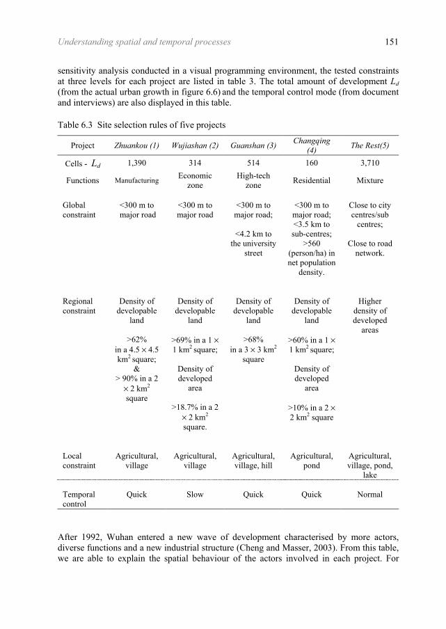
The land cover transition from 1993 to 2000 shown in table2 is calculated based on a 10×10 m2 cell size. This table shows that major land use/cover changes come from water, town/villages and agricultural land, which were physically or functionally transferred into the urban built-up area. Town/villages with the highest annual transition rate were only functionally transferred to urban administration due to the rapid expansion of Wuhan municipality. Agricultural land has the highest transition percentage. Here, the water body includes ponds and lakes. A higher percentage area is taken for transition from ponds than from lakes (see map of actual pattern in figure 6.6). The item 'Others' includes green areas, sands, and mis-classification from image processing etc, which is omitted for modelling. 6.3.2 Project planning and site selection With the assistance of historical documents, local planners and fieldwork, four large-scale projects, planned before or around 1993 were identified (WBUPLA, 1995). All small-scale projects were merged into one class, which results in five projects (figure 6.6 and table 6.3) as follows: 1) Zhuankou: car manufacturing plant (planned from 1988); 2) Wujiashan: Taiwanese investment zone (planned from 1992); 3) Guanshan: hi-tech development zone (planned from 1988); 4) Changqing: large-scale residential zone (planned from 1994); 5) The rest: small-scale development (commercial/institutional/residential). In a GIS environment (ArcView 3.2a), we create the required spatial layers (figure 6.5), including land cover of 1993, distance to road networks and city centres/sub-centres, and population density. These layers are exported into a computational program for testing different site selection rules for each project according to equation 2. As a result of a


151

sensitivity analysis conducted in a visual programming environment, the tested constraints at three levels for each project are listed in table 3. The total amount of development Ld (from the actual urban growth in figure 6.6) and the temporal control mode (from document and interviews) are also displayed in this table. Table 6.3 Site selection rules of five projects

Project Zhuankou (1) Wujiashan (2) Guanshan (3) Changqing (4) The Rest(5)

Cells - Ld 1,390 314 514 160 3,710

Functions Manufacturing Economic zone

High-tech zone Residential Mixture

Global constraint

<300 m to major road

<300 m to major road

<300 m to

major road;

<4.2 km to the university

street

<300 m to

major road; <3.5 km to sub-centres;

>560 (person/ha) in net population

density.

Close to city centres/sub

centres;

Close to road network.

Regional constraint

Density of

developable land

>62%

in a 4.5 × 4.5 km2 square;

& > 90% in a 2

× 2 km2

square

Density of

developable land

>69% in a 1 × 1 km2 square;

Density of developed

area

>18.7% in a 2 × 2 km2 square.

Density of

developable land

>68%

in a 3 × 3 km2

square

Density of

developable land

>60% in a 1 × 1 km2 square;

Density of developed

area

>10% in a 2 × 2 km2 square

Higher

density of developed

areas

Local constraint

Agricultural,

village

Agricultural,

village

Agricultural, village, hill

Agricultural,

pond

Agricultural, village, pond,

lake Temporal control

Quick

Slow

Quick

Quick

Normal

After 1992, Wuhan entered a new wave of development characterised by more actors, diverse functions and a new industrial structure (Cheng and Masser, 2003). From this table, we are able to explain the spatial behaviour of the actors involved in each project. For

Chapter 6

152

instance, the dominant actor in the Zhuankou, Wujiashan and Guanshan projects is Wuhan municipality, which obtained financial resources from the central government, foreign investors and local enterprises. Being the owner of the land, the actor did not need to consider the costs of land utilisation. Hence, for large-scale projects, the first rule is the availability of a certain amount of developable land. Being oriented towards manufacturing and tertiary industry, the second rule is accessibility to major road networks. Strictly speaking, the second one is not only true for large-scale but also for small-scale land development such as commercial use. Moreover, accessibility to developed areas is crucial for the economic development zone (Wujiashan) and the high-tech zone (Guanshan). Access to research resources, including nearly 20 universities is a prerequisite to locating a high-tech zone (Guanshan). In contrast, the major actors in the Changqing housing project are local real estate companies and relevant work units. Land value is becoming an important criterion, which weakens the role of accessibility to the city centres. The low-quality land cover such as ponds is much cheaper than agricultural land. Higher population density can guarantee better market demand as an influential factor for residential development. For small-scale projects, especially inside urban districts, more actors are involved in the decision-making, including local residents, investors, work units, planners and the lower levels of local government. This results in a more stochastic process of site selection as a result of which the constraints become more uncertain and fuzzy. However, generally speaking, accessibility to the city centre/sub-centre and road networks is the key factor. 6.3.3 Local growth The cell size in this research is 100 × 100 m2, which results in a 640 × 410 grid. A smaller cell size (such as 10 × 10 m2) would cause an overload in terms of model computation. The state of cells is binary (1 - change, 0 - nonchange). The initial layer is the 1993 land cover. This includes Developed, Agricultural (A), Village/town (V), Pond (P), Lake (L), and Protected (Green, Park, and Sands). In figure 6.5a, P and L are merged into water bodies, and 'others' include protected. As described in 6.3.1, only four types A, V, P and L, underwent much change. The pattern model from another part of this research (Cheng and Masser, 2003), shown that the major spatial determinants of urban growth in 1993-2000 included major road networks, minor road networks, centres/sub-centres and master planning (as displayed in figure 6.5). They are selected here as non-constrictive factors for evaluating the potential for land conversion. It should be noted that the classification of each layer is of great importance and modelling is sensitive to the classification, particularly when the study area is large and the period is long. For instance, the construction of roads may occur in different phases of the period to be modelled. Their construction time should be taken into account. In this research, a major road connection (linking with the Third Bridge over the Yangtze River) was completed in early 2000. This is clearly visible in the 2000 SPOT images. However, this major road is not included in the major road network layer because it had no practical impacts on urban development in the period 1993-2000. This judgement is also confirmed by very sparse and

Figu

re 6

.4

Spat

ial

fact

ors

and

cons

train

ts fo

r si

te s

elec

tion

and

CA

mod

ellin

g: a

) la

nd c

over

of

1993

; b)

pop

ulat

ion

dens

ity(p

erso

ns/h

a); c

) roa

d ne

twor

ks a

nd c

entre

s/su

b-ce

ntre

s; d

) mas

ter p

lan

1996

-202

0.

(d)

(c)

(a)

(b)

Chapter 6

154

limited land cover change surrounding the road. Other layers are spatially defined by the following similar rules. Wuhan city can be treated as a flat landscape as its elevation ranges between 22 and 27 m above sea level apart from a few hills. Hence, slope is not an influential factor. Physical constraints principally comprise water bodies (see figure 6.5a). Theoretically, water bodies should be completely excluded. However, in this case study, 18% of the land cover change comes from water bodies, which include ponds and lakes (see table 6.2). As this comes mostly from either small-scale ponds or the fringe of large lakes, a general procedure can be designed for defining a specific layer (exclusion layer): • Extracting a water body from the land cover layer of 1993; • Neighbourhood statistics (based on a circular neighbourhood with a 200 m radius); • Selecting sum > 4 (neighbouring 4 ha area is water) The layer will be utilised as physical constraint from the water body, defining excluded zones from transition. In the five CA models corresponding to the five projects, a circular neighbourhood is chosen because it does not have significant directional distortion. Its size varies with different projects, ranging from three to nine cells. The selection of neighbourhood size for each project relies on empirical study and sensitivity analysis (see a later section). The heterogeneity of spatial processes is indicated by the varied combination of influential factors, weight values and parameters, which imply distinguishing local spatial behaviour. Table 6.4 Influential degree of master planning on land cover transition

Code Classification Zhuankou Ci / Mi Mi

Guanshan Ci / Mi Mi

The Rest Ci / Mi Mi

R1 Low-rise residential 0.237 265 0.23 57 0.087 1082 R3 Poorer environment - - - - 0.1333 149 M Industry 0.318 508 0.24 172 0.049 419 G1 Public green 0.27 137 - - 0.0916 416 G2 Protected land 0.147 58 0.33 112 0.041 222 G3 Ecological agriculture - - - - 0.0216 82 C1 Administration/Offices 0.26 52 - - 0.0787 17 C3 Cultural/Recreational 0.528 16 - - - - C4 Sports facility - - 0.3 44 0.035 89 C5 Hospital/Health 0.742 33 - -, - - S1 Street - - - - 0.069 354

"-": Mi <15 (omitted) Given that local growth is impacted by the master plan to be implemented in this period, we must incorporate the master plan for 1996-2020 as an influential factor (this scheme was initiated in 1990 and approved by the central government in 1996). Due to the rapid urban expansion in the fringe, some projects such as Changqing and Wujiashan had not even been planned until their construction. These will be excluded from the master planning analysis.


155

Only the projects covered by master planning are considered i.e. Guanshan, Zhuankou and The Rest. Each cell j is assigned a value Xj, representing the influential degree of the planned land use on its land cover transition in a project. If Mi denotes the total area of land use i in a specific project, Ci denotes the transited part of Mi, Ci / Mi generally indicates the influential degree of land use i. If a cell j was planned as land use i, Xj =Ci / Mi . Xj needs to be standardised according to equation 4 (Xj-min) / (max-min) before it can be incorporated into the evaluation formula (equation 3). The Mi and Ci / Mi values of the major land uses are listed in table 6.4. The item 'Code' follows the National Urban Land Use Classification Standard (NULCS). Generally, table 6.4 reveals that the master plan was more successful in guiding large-scale projects in the fringe than small-scale ones in urban districts. In figure 6.5d, "Residential" includes R1~R3, "Green" G1~G3, "Street" S1, and the rest (C1, C3, C4, C5) are all merged into "Others". The calibration of parameters has proved a difficult task in urban CA modelling (Clarke and Gaydos, 1998; Li and Yeh, 2001a), especially when there are many factors and parameters to be considered. The difficulty lies in the fact that most urban CA modelling takes the whole municipality into the calibration procedure, which results in intensive computation overload. In this research, project-based CA modelling has largely reduced the computational time of calibration as the spatial extent of the project is much smaller than the whole study area, as shown in table 6.5 and figure 6.6. The factors and parameters for model calibration include six spatial factors, neighbourhood size and stochastic disturbance α. Other parameters (e.g. temporal pattern mode parameter λ, iteration time t) are utilised for sensitivity analysis in section 6.4.1. The six spatial factors are "distance to minor road" (OR), "distance to major road" (MR), "distance to centre/sub-centres" (CN), "density of neighbouring developed areas" (DD), "density of neighbouring new development" (DN), and "master planning". Their parameters φ (in equation 5) are taken from the global pattern model of logistic regression carried out in another part of this research (Cheng and Masser, 2003). Automatic search for the best-fit parameters is carried out by using a hierarchical means, i.e. to reduce step size for five loops corresponding to six factors at two stages. For example, the step size of loops in calculating the weight values is set as 0.05 first, i.e. from 0.05 to 1 step 0.05. When the parameter scope of the ideal accuracy is determined, e.g. from 0.2 to 0.25, we can set a second step size 0.005 for finer calibration, i.e. from 0.2 to 0.25 step 0.005. The validation accuracy depends on the approach used to compare simulated and actual patterns. This is traditionally measured by a coincidence matrix generated by a cell-cell comparison of two pattern maps. Some researchers argue that CA simulations should be assessed not just on the goodness of fit (a cell by cell basis) but also on their feasibility and plausibility as urban systems are rather complicated and their exact evolution is unpredictable (Wu and Webster, 1998; White and Engelen, 2000; Yeh and Li, 2001a). Some global measures that have been used for testing the validity of CA simulation include the fractal and Moran I index (Wu, 1998a), fractal analysis (Yeh and Li, 2001a), and landscape metrics (Soares-Filho et al., 2002). Wu (2002) emphasises the need to validate the model through both structural and cross-tabulation measures. Structural measures can only compare the pattern (outcome of process) not the spatial location (or process).

Chapter 6

156

Table 6.5 CA Simulation of five projects

Projects Zhuankou-1

Zhuankou-2 Wujia shan

Guan shan

Changqing

Rest

Land demand Ld 1,390 1,390 314 514 160 3,710 Accuracy CC 54% 54% 51.6% 53.2% 85% 55% Lee-Sallee index 0.37 0.37 0.35 0.36 0.74 0.38 Neighbourhood size 6 6 5 8 3 7 λ 4/3 4/3 4 4/3 4/3 2 Dynamic weighting - <15% 15-55% >55% - - - - Major road (MR) 0.2 - 0.5 0.05 0.325 - 0.1 0.3 Minor road (OR) 0.3 - 0.1 0.15 0.1 0.35 0.55 0.15 Centres (CE) - 0.7 - 0.5 - - - 0.2 Neighbourhood-new 0.3 0.3 0.1 0.15 0.3 0.35 0.35 0.1 Neighbourhood-old - - - - 0.275 0.25 - 0.2 Master planning 0.2 - 0.3 0.15 - 0.05 - 0.05 Total 100% 100% 100% 100% 100% 100% 100% 100%

Note: α=1%, n=50, φ for MR, OR and CN: 0.000765, 0.0012 and 0.000272 Figure 6.5 Simulated (1994-2000 in order) and actual patterns (last map)


157

We consider that spatially location match is also of great importance for supporting planning decision-making despite the difficulties imposed by CA modelling. Another reason lies in the fact that local processes at the project level require more accurate cell-based measures, as their morphology is less definite than that of processes at the global level. Clarke and Gaydos (1998) outline four ways to statistically test the degree of historical fit (three r-squared fits and one modified Lee-Sallee shape index). For the Lee-Sallee shape index (combining the actual and the simulated distributions as binary urban/non-urban, and computing the ratio of the intersection over the union), they reported that the practical accuracy is only 0.3. In this chapter, we use consistency coefficients (CC) (the percentage of the matched over the actual) and the Lee-Sallee index (LI) for the evaluation of goodness of fit. The total number of pixels is set the same for simulation as the actual pattern, i.e. Ld = Ln, LI=CC/(2-CC). For example, when CC=0.57, LI=0.4. Following this formula, the Lee-Sallee index for five projects are computed and listed in table 6.5. The overall accuracy based on the weighted combination (Ld) of five projects is 0.554 in CC and 0.383 in LI, greater than those of Clarke. 6.3.4 Temporal control With local knowledge, we are able to identify the patterns of temporal development of each project (see table 6.3). In 1993, Zhuankou was still completely rural. By 1995 it was nearly half constructed. There was not much change from 1997 and 2000. Therefore, its temporal growth pattern is defined as "Quick". The small-scale projects (the Rest) are a mixture of all three patterns. Some may be quick and others slow. On average, it is reasonable to classify them as "Normal". The number of iterations is defined as n=50 because the greater the number, the finer the discriminative capacity of the models. Figure 6.6 exhibits the trajectories of temporal development of the five projects respectively, according to the results of the validated CA simulation. As described in equation 12, the output of CA simulation is Li(t) (1~n), which is different from the yearly actual amount Li(y) (1~m) for each project i. We need a transition from Li(t) to Li(y). The transition function h in equation 12 should be based on an understanding of the actual temporal development process, which is determined by its socio-economic development. For the sake of simplicity, we use an equal time interval, i.e. a linear function: y = t/7. As t ranges from 1 to 50 (n=50) and y from 1 to 7 (m=7), Li(y)= ΣLi(t), t from 7*(y-1)+1 to 7*y. A series of newly created layers for the whole study area, corresponding to the seven-year urban growth (from 1993 to 2000, figure 6.6), have been imported into animation software (Animagic32) for dynamic visualisation. This animation is helpful for exploring and comparing the temporal dynamics of spatial processes.

Chapter 6

158

Table 6.5 shows the spatial heterogeneity of the causal factors, which vary spatially in terms of their weight values. The neighbourhood effect is represented by neighbourhood size, and the weight values of new and old developed areas. This table suggests that there are some similarities and some dissimilarities between the five projects. The weight values of the major roads, minor roads, city centre/sub-centres and master planning also show some differences. Major roads play a greater role in "The Rest" and Wujiashan, and less important roles in Changqing and Guanshan. Conversely, minor roads play a greater role in the latter projects than in the former. By linking the site selection rules shown in table 6.3, it can be seen that the road networks system actually takes varying roles during different phases of urban growth. The major road network is the key at the stage of site selection and remains important for some areas at the stage of local growth. However, the minor road network is only active at the stage of local growth. This is due to the fact that minor road networks are created after the stage of site selection, together with the new growth. Relatively, city centres/sub-centres are influential only for "The Rest" as the others are located in the urban fringe. Master planning is less influential than others. The spatial heterogeneity described above suggests that the causal effects of urban growth vary from place to place. Local process modelling can offer deeper insights into urban growth processes.

Figure 6.6 Temporal control patterns of five projects

-500

0

500

1000

1500

2000

2500

3000

3500

4000

1 5 9 13 17 21 25 29 33 37 41 45 49

The RestChangqingZhuankouGuanshanWujiashan

Lt

t


159

6.3.5 Local temporal dynamics Local temporal dynamics are focused on each project and are indicated by the following examples: • Compared with the major road network, minor roads, especially in new zones that are

also new development units, may occur temporally at different phases of the period studied, i.e. between T0 and Tn, but not immediately from T0;

• The spatial impacts of various factors such as roads and centres are not simultaneous in temporally affecting local growth;

• Neighbourhood effects may suffer from temporal variation; for example, it may be stronger at T0 than at Tn, or vice versa.

These examples qualitatively show the complex pattern and process interaction as explained in section 6.2.4. Two models of Zhuankou in table 6.5 have similar model accuracy and similar patterns. However, their spatial-temporal processes are quite different, as quantitatively shown in figure 6.8. Model 1 exhibits a more random process. Model 2 shows a more self-organised process. Model 2 is based on the assumption that new development in Zhuankou first occurred in the centre, then along the major road, and finally spread from the centre. The assumption corresponds to a temporal dynamics that is spatially controlled by three sets of weight values (table 6.5). To calibrate this process-oriented CA model, manual tests based on the modeller's understanding of local growth processes and the visual exploration of model outputs (temporal patterns) are very important for reducing parameter ranges and making rough estimates of dynamic weight values. Limited automatic search can be followed for the best ideal combination of parameters.

Figure 6.7 Local temporal dynamics (Zhuankou-1 and -2 in table 6.5)

Chapter 6

160

To some extent, the dynamic weighting implies the temporal lag of the spatial influences of locational factors on urban growth. This example suggests that local temporal dynamics can enable us to better understand the organised local growth. If we explore the changes in weight values, it can be found that the major changes are indicated in major roads and centres. As explained in equation 13, the weight values should be non-linear functions of temporal land development demand. Table 6.5 also shows the functions are highly complex in reality. They are frequently phased. Model 2 is actually based on local knowledge. Other projects can be calibrated temporally by the same procedures as in the Zhuankou project. 6.4 Discussion and Conclusions 6.4.1 Model calibration and validation Li and Yeh (2001a) report a calibration procedure of CA modelling by using an artificial neural network. In their method, the neural network is utilised to obtain the optimal parameter values automatically based on training empirical data, and then the parameter values calibrated are used to carry out CA simulation for new data. In CA models of this kind, the transition rules represented by the neural network structure are not transparent to users. Consequently, this method can be used for prediction by using the same set of rules, but it is not ideal for interpreting the logic of land conversion or spatial-temporal processes as it is a black box (Wu, 2002). It has been found in this research that visual tests offer a quick and useful way of calibrating and verifying a CA model (Clarke et al., 1997; Ward et al., 2000a), particularly with respect to sensitivity analysis. In this project-based CA modelling, calibration has proved not to be a severe problem in computation time. However, the optimal combination of parameters from automatic search may not give the best results as socio-economic systems essentially produce no best solution. Consequently, the calibrated results need further confirmation according to the interpretation and plausibility of their spatial and temporal processes. In table 6, the Wujiashan project is taken as an example to illustrate this issue. When neighbourhood size is set as 5, the optimal parameters with 52.8% accuracy are calculated by automatic search (step of weight value is 0.005), together with the other combination of parameters. However, the spatial processes produced by the weight values (0.2, 0.1, 0.45, 0.25) are not the same as the real temporal pattern based on visual comparison. Conversely, another combination (0.325, 0.1, 0.3, 0.275) can create more satisfactory temporal patterns, although its model accuracy (51.6% in CC) is lower. Consequently, visual tests are still a necessary means for process rather than pattern modelling.


161

Table 6.6 Calibration of CA modelling and sensitivity analysis (Wujiashan project) Accuracy CC(%) 52.8 51.6 51.3 50.8 29.5 46 49.7 50 50.8 Neighbourhood size 5 5 5 5 5 8 6 4 5

λ=4.5 Major road (MR) 0.2 0.325 0.325 0.225 0.375 0.1 0.325 0.325 0.325 Minor road (OR) 0.1 0.1 0.05 0.25 0.3 0.3 0.1 0.1 0.1 Neighbourhood (new) 0.45 0.3 0.35 0.15 0.3 0.4 0.3 0.3 0.3 Neighbourhood (old) 0.25 0.275 0.275 0.375 0.025 0.2 0.275 0.275 0.275 Total (%) 100 100 100 100 100 100 100 100 100

Note: α=1%, n=50, λ=4, φ for MR, OR and CN: 0.000765, 0.0012 and 0.000272 Another part of calibration is sensitivity analysis, as the results of CA simulation are very sensitive to the parameter values (e.g. neighbourhood size, weight values, λ and n). This is the issue of uncertainty existing in CA simulation that has not been given enough attention in most applications. For the Wujiashan project, before accepting (0.325, 0.1, 0.3, 0.275), we need to test its stability by slightly or greatly adjusting the weight values and the other parameters such as neighbourhood size as listed in table 6.6. The changes (slight or great) in validation accuracy that are identical to those in parameters assure the reliability of this set. 6.4.2 Visualisation of processes To implement site selection and CA modelling, a loose coupling strategy is frequently adopted for various applications (Clarke and Gaydos, 1998; Bell et al., 2000). Loose coupling means that a data transfer procedure is frequently implemented between a CA model, GIS, and an animation module. This loose coupling strategy sacrifices the friendly interface but improves the computation efficiency of CA simulation. Here the site selection rules and the CA model is programmed in object-oriented programming language. Spatial data analysis and visual exploration tasks are implemented within a GIS environment − ArcView platform. Each layer produced is exported as an ASCII raster file. A sub-procedure is programmed to read and write the ASCII raster files between CA and ArcView. The major parameters include the weight values, the temporal pattern control λ, the neighbourhood size and the stochastic perturbation α. The validation results are stored in a text file and an ASCII raster file. A validated urban growth layer (1993-2000) from the simulation is separated into a series of maps, each corresponding to one year. The layers created are exported as a JPG or any other type of image file. These are inserted as an individual frame into the animation file for visual check of the spatial process. However, a major deficiency of this strategy is that it is not a very friendly environment for the immediate visualisation of spatial-temporal processes, although it is effective for model calibration. In the future, CA modelling tightly coupled with GIS and animation should be further studied to enhance its visualisation of spatial-temporal processes.

Chapter 6

162

6.4.3 Process modelling To some extent, the accuracy of a simulation model depends on the complexity and stochasticity of the real city and also on the availability of more detailed information. Although the overall accuracy of five CA models is only 55% based on a cell by cell basis, the methodology proposed in this chapter illustrates the potential for understanding spatial processes and their temporal dynamics at the two levels based on the methodology. The spatial clustering of land development projects indicates a self-organising process. The timing schedule of various projects exhibits global temporal dynamics. Dynamic weighting is an important concept for simulating process rather than pattern. Spatial classification based on the project concept is subjective but transparent to urban planners. The spatial-temporal processes explored by project-based modelling can easily be interpreted with reference to socio-economic and decision-making processes. To be a true process model, CA modelling as suggested in this research should incorporate dynamic weighting methods, although there is still much difficulty in systematically defining these functions in practice. From the local spatial modelling point of view, a possible direction lies in applying a moving window or kernel in defining a project for each cell, so that generalised local process modelling can be repeatedly applied for each cell. This is a similar principle to that applied in geographically weighted regression (GWR) modelling. This idea can result in universally localised process modelling. The parameters for understanding local processes vary with the cell. Users can redefine interesting projects for further interpretation by focusing on some hot spots. From the perspective of spatial data analysis, the methodology can be utilised to discover the hidden processes from the required integrated spatial database regarding temporal urban growth. This has been one of the major concerns in the field of spatial data mining or knowledge discovery. When socio-economic data at detailed levels become available, project-based CA modelling can be further linked with micro-scale multi-agent and economic modelling. Such integration can explore the spatial and economic behaviour of various actors at the micro scale. The major purpose of CA simulation is to generate alternative scenarios for decision support in a smart growth management. The methodology developed here can be extended in this direction. In this new case, stages 1 and 4 need to incorporate top-down socio-economic models for predicting the demand for new land development in the future, i.e. Ld in equation 1. Stages 2 and 3 are subject to some modification in quantification. The construction of plan scenarios is based on soft systems thinking, which stresses the role of users' subjectivity. In this way local planners' intentions can be transformed into spatially and temporally explicit weight values and certain parameters (e.g. Wu, 1998c). With a user-friendly visualisation environment, the framework tested in this research can facilitate decision-making of urban spatial development. We cannot ignore the fact that any advanced modelling technique including CA must be based on a proper understanding and abstraction of the systems studied. The better the understanding the more accurate it is likely to be. Planning will never be a hard science, for


163

it is built on humanistic assumptions, values and goals (Shmueli, 1998). Our understanding of the new urban reality will be ultimately based upon a combination of computers and human judgement (Sui, 1998). CA is only a simulation tool for testing a decision-maker's understanding. Limited by existing GIS theory and methods, the identification of various spatial and temporal heterogeneity cannot be completed without the assistance of local knowledge. This implies that local knowledge is an important ancillary data source for CA modelling especially within the framework presented in this chapter. During the process of the modelling, project planning, site selection and temporal control need more input from local experts. For dynamic weighting, due to the limited temporal resolution, local knowledge is an essential source of qualitative information. It has been emphasised in this research that a soft system methodology, stressing the roles of decision-makers and feedback both between modellers and users and between stages of the decision-making process, is helpful, especially when complete information resources are not guaranteed.

chapter 6 understanding spatial and temporal processes of ......linear function of temporal land...

Documents