ch.1. description of motion
TRANSCRIPT

CH.1. DESCRIPTION OF MOTION Multimedia Course on Continuum Mechanics
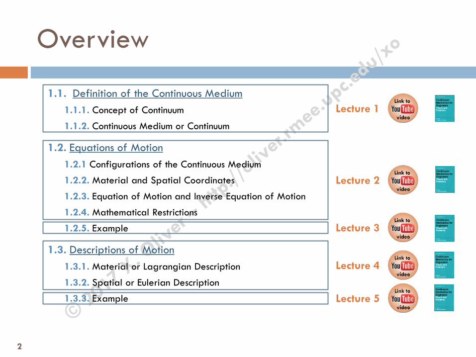
Overview
1.1. Definition of the Continuous Medium 1.1.1. Concept of Continuum
1.1.2. Continuous Medium or Continuum
1.2. Equations of Motion 1.2.1 Configurations of the Continuous Medium
1.2.2. Material and Spatial Coordinates
1.2.3. Equation of Motion and Inverse Equation of Motion
1.2.4. Mathematical Restrictions
1.2.5. Example
1.3. Descriptions of Motion 1.3.1. Material or Lagrangian Description
1.3.2. Spatial or Eulerian Description
1.3.3. Example
2
Lecture 5
Lecture 1
Lecture 2
Lecture 4
Lecture 3

Overview (cont’d)
1.4. Time Derivatives 1.4.1. Material and Local Derivatives
1.4.2. Convective Rate of Change
1.4.3. Example
1.5. Velocity and Acceleration 1.5.1. Velocity
1.5.2. Acceleration
1.5.3. Example
1.6. Stationarity and Uniformity 1.6.1. Stationary Properties
1.6.2. Uniform Properties
3
Lecture 6
Lecture 7
Lecture 10
Lecture 9
Lecture 8

Overview (cont’d)
1.7. Trajectory or Pathline 1.7.1. Equation of the Trajectories 1.7.2. Example
1.8. Streamlines 1.8.1. Equation of the Streamlines 1.8.2. Trajectories and Streamlines 1.8.3. Example 1.8.4. Streamtubes
1.9. Control and Material Surfaces 1.9.1. Control Surface
1.9.2. Material Surface
1.9.3. Control Volume
1.9.4. Material Volume
4
Lecture 12
Lecture 11

Ch.1. Description of Motion
1.1 Definition of the Continuous Medium
5

The Concept of Continuum
Microscopic scale: Matter is made of atoms which may be grouped in
molecules.Matter has gaps and spaces.
Macroscopic scale: Atomic and molecular discontinuities are disregarded.Matter is assumed to be continuous.
6

Continuous Medium or Continuum
Matter is studied at a macroscopic scale: it completely fills the space, there exist no gaps or empty spaces.
Assumption that the medium and is made of infinite particles (of infinitesimal size) whose properties are describable by continuous functions with continuous derivatives.
7

Exceptions to the Continuous Medium
Exceptions will exist where the theory will not account for all the observed properties of matter. E.g.: fatigue cracks. In occasions, continuum theory can be used in combination
with empirical information or information derived from aphysical theory based on the molecular nature of material.
The existence of areas in which the theory is not applicable does not destroy its usefulness in other areas.
8
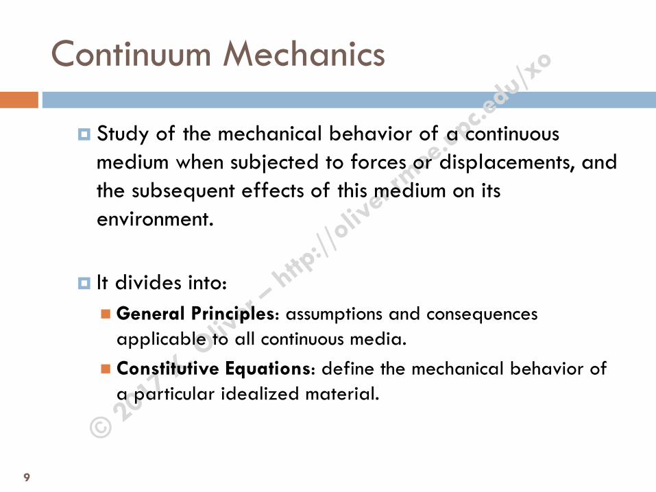
Continuum Mechanics
Study of the mechanical behavior of a continuous medium when subjected to forces or displacements, and the subsequent effects of this medium on its environment.
It divides into: General Principles: assumptions and consequences
applicable to all continuous media. Constitutive Equations: define the mechanical behavior of
a particular idealized material.
9

Ch.1. Description of Motion
1.2 Equations of Motion
10

Material and Spatial points, Configuration
A continuous medium is formed by an infinite number of particles which occupy different positions in space during their movement over time.
MATERIAL POINTS: particles
SPATIAL POINTS: fixed spots in space
The CONFIGURATION Ωt of a continuous medium at a given time (t) is the locus of the positions occupied by the material points of the continuous medium at the given time.
11

Γ0
Ω0 X
Ω
Γ
x
( ), tϕ X
Configurations of the Continuous Medium
Ω or Ωt: deformed (or present) configuration, at present time t.
Γ or Γt : deformed boundary. x : Position vector of the same
particle at present time.
Ω0: non-deformed (or reference) configuration, at reference time t0.
Γ0 : non-deformed boundary. X : Position vector of a particle at
reference time.
Initial, reference or undeformed configuration
Present or deformed configuration
0 0t = → reference time [ ]0,t T∈ → current time
12

Material and Spatial Coordinates
The position vector of a given particle can be expressed in: Non-deformed or Reference Configuration
Deformed or Present Configuration
[ ]1
2
3
XX XX YX Z
= = ≡
material coordinates (capital letter)
[ ]1
2
3
xx xx yx z
= = ≡
spatial coordinates (small letter)
13

The motion of a given particle is described by the evolution of its spatial coordinates (or its position vector) over time.
The Canonical Form of the Equations of Motion is obtained when the “particle label” is taken as its material coordinates
Equations of Motion
( ) ( )( )
, ,
, 1, 2,3i i
t t
x t i
ϕ
ϕ
= =
= ∈
x xparticle label particle label
particle label
φ (particle label, t) is the motion that takes the body from a reference configuration to the current one.
1 2 3TX X X≡ ≡ Xparticle label
( ) ( )( ) 1 2 3
, ,
, , , 1,2,3
not
i i
t t
x X X X t i
x X x Xϕ
ϕ
= =
= ∈
14

Γ0
Ω0 X
Ω
Γ
x
( ), tϕ X
( )1 ,x tϕ−
Inverse Equations of Motion
The inverse equations of motion give the material coordinates as a function of the spatial ones.
( ) ( )( )
1
11 2 3
, ,
, , , 1,2,3
not
i i
t t
X x x x t i
X x X xϕ
ϕ
−
−
= =
= ∈
15

Mathematical restrictions for φ and φ-1 defining a “physical” motion
Consistency condition , as X is the position vector for t=0
Continuity condition , φ is continuous with continuous derivatives
Biunivocity condition φ is biunivocal to guarantee that two particles do not occupy
simultaneously the same spot in space and that a particle does not occupy simultaneously more than one spot in space. Mathematically: the “Jacobian” of the motion’s equations should be different from zero:
The “Jacobian” of the equations of motion should be
“strictly positive”
( ),0ϕ =X X
1Cϕ∈
( ),det 0i
j
tJ
ϕ ϕ ∂ ∂= = >
∂ ∂
XX X
( ),det 0i
j
tJ
ϕ ϕ ∂ ∂= = ≠
∂ ∂
XX X
16
density is always positive (to be proven)

Example
The spatial description of the motion of a continuous medium is given by:
Find the inverse equations of motion.
( )
2 21 1
2 22 2
2 23 1 3
,5 5
t t
t t
t t
x X e x Xet x X e y Ye
x X t X e z Xt Ze
− −
= = ≡ = ≡ = = + = +
x X
17

Example - Solution
Check the mathematical restrictions:
Consistency Condition ?
Continuity Condition ?
Biunivocity Condition ?
Density positive ?
( ),0ϕ =X X
1Cϕ∈
( ),0
tJ
ϕ∂= >
∂XX
( )
21 1
22 2
23 1 3
,5
t
t
t
x X et x X e
x X t X e
−
=
≡ = = +
x X
( )
2 01 1
2 02 2
2 01 3 3
, 05 0
X e Xt X e X
X X e X
⋅
− ⋅
⋅
= = = = ⋅ +
x X X
1 1 1
21 2 3
2 2 2 2 22 2 2
1 2 3 2
3 3 3
1 2 3
0 00 0 05 0
t
t t t t ti
j t
x x xX X X
ex x x xJ e e e e e tX X X X
t ex x xX X X
− −
∂ ∂ ∂∂ ∂ ∂
∂ ∂ ∂ ∂= = = = ⋅ ⋅ = ≠ ∀∂ ∂ ∂ ∂
∂ ∂ ∂∂ ∂ ∂
2 0tJ e= >
18

Example - Solution
Calculate the inverse equations:
( )
21 1
22 2
23 1 3
,5
t
t
t
x X et x X e
x X t X e
−
=
≡ = = +
x X
2 211 1 1 12
t tt
xx X e X x ee
−= ⇒ = =
2 222 2 2 22
t tt
xx X e X x ee
−−= ⇒ = =
( )( )2 2 2 2 43 13 1 3 3 3 1 3 12
55 5 5t t t t tt
x X tx X t X e X x x e t e x e tx ee
− − − −−= + ⇒ = = − = −
( )
21 1
1 22 2
2 43 3 1
,5
t
t
t t
X x et X x e
X x e tx eϕ
−
−
− −
=
≡ = = = −
X x
19

Ch.1. Description of Motion
1.3 Descriptions of Motion
20

Descriptions of Motion
The mathematical description of the particle properties can be done in two ways: Material (Lagrangian) Description
Spatial (Eulerian) Description
21
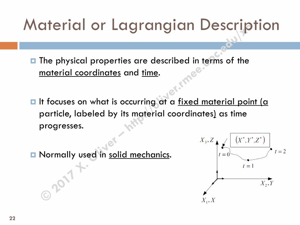
Material or Lagrangian Description
The physical properties are described in terms of the material coordinates and time.
It focuses on what is occurring at a fixed material point (a particle, labeled by its material coordinates) as time progresses.
Normally used in solid mechanics.
22

The physical properties are described in terms of the spatial coordinates and time.
It focuses on what is occurring at a fixed point in space (a spatial point labeled by its spatial
coordinates) as time progresses.
Normally used in fluid mechanics.
Spatial or Eulerian Description
23

Example
The equation of motion of a continuous medium is:
Find the spatial description of the property whose material description is:
( ), x X Yt
t y Xt Yz Xt Z
= −= ≡ = + = − +
x x X
( ) 21X Y ZX,Y,Z,t
tρ + +
=+
24

Example - Solution
Check the mathematical restrictions:
Consistency Condition ?
Continuity Condition ?
Biunivocity Condition ?
Any diff. Vol. must be positive ?
( ) XX =0,φ
1C∈φ
( ) 0,>
∂∂
=XX tJ φ
( )0
, 0 00
X Y Xt X Y Y
X Z Z
− ⋅ = = ⋅ + = = ⋅ +
x X X
( ) 2
1 01 0 1 1 1 1 1 00 1
i
j
x x xX Y Z t
x y y yJ t t t t tX X Y Z
tz z zX Y Z
∂ ∂ ∂∂ ∂ ∂ −
∂ ∂ ∂ ∂= = = = ⋅ ⋅ − ⋅ − ⋅ = + ≠ ∀∂ ∂ ∂ ∂
−∂ ∂ ∂∂ ∂ ∂
21 0J t= + >
( ), x X Yt
t y Xt Yz Xt Z
= −= ≡ = + = − +
x x X
25

Example - Solution
Calculate the inverse equations:
( ), x X Yt
t y Xt Yz Xt Z
= −= ≡ = + = − +
x x X
221
x X Yt X x Yty Y y xtx Yt Yt Y y xt Yy Y t ty Xt Y X
t
= − ⇒ = + − −⇒ + = ⇒ + = − ⇒ =− += + ⇒ =
2 2
2 2 21 1 1y xt x xt yt xt x ytX x Yt x t
t t t− + + − + = + = + = = + + +
2 2
2 21 1x yt z zt xt ytz Xt Z Z z Xt z t
t t+ + + + = − + ⇒ = + = + = + +
( )
2
12
2 2
2
1
,1
1
x ytXt
y xtt Yt
z zt xt ytZt
ϕ−
+ = +−≡ = = +
+ + += +
X x
26

Example - Solution
Calculate the property in its spatial description:
( )( )
2 2
2 2 2 2 2
22 2 2
1 1 11 1 1
x yt y xt z zt xt ytt t tX Y Z x y yt yt z ztX,Y,Z,t
t t tρ
+ − + + + + + + + ++ + + + + + + = = =+ + +
( )
2
12
2 2
2
1
,1
1
x ytXt
y xtt Yt
z zt xt ytZt
ϕ−
+ = +−≡ = = +
+ + += +
X x
( ) ( ) ( )( )
( )2 2
22 2
1 1
1 1
x y t t z tX Y ZX,Y,Z,t x, y,z,tt t
ρ ρ+ + + + ++ +
= ⇒ =+ +
27

Ch.1. Description of Motion
1.4 Time Derivatives
28

Material and Local Derivatives
The time derivative of a given property can be defined based on the: Material Description Γ(X,t) TOTAL or MATERIAL DERIVATIVE
Variation of the property w.r.t. time following a specific particlein the continuous medium.
Spatial Description γ(x,t) LOCAL or SPATIAL DERIVATIVE Variation of the property w.r.t. time in a fixed spot of space.
( ), tt
∂Γ ≡ → ∂
X partial time derivative of the material derivative
of the properymaterial description
( ), tt
γ∂ ≡ → ∂
x partial time derivative of the local derivative
of the properyspatial description
29

Convective Derivative
Remember: x=x(X,t), therefore, γ(x,t)=γ(x(X,t),t)=Γ(X,t) The material derivative can be computed in terms of
spatial descriptions:
Generalising for any property:
( ) ( )
( )( ) ( )
( )
( , ) ( , )( , ) ( , )
( , ), ,
, ,, ,
not not
i
i
i t it t
t t
d D tt tdt Dt tt txd t t
dt t x t t tγγ
γ
γ γ
γ γγ γγ
∂∂ ⋅
∂Γ→ = = = =
∂∂ ∂∂∂ ∂ ∂
= = + ⋅ = + ⋅ =∂ ∂ ∂ ∂ ∂ ∂
x x v xv x x
Xx x
x x xx Xx
material derivative
∇∇∇
( ) ( ) ( ) ( ), ,, ,
d t tt t
dt tχ χ
χ∂
= + ⋅∇∂
x xv x x
REMARK The spatial Nabla operator is defined as: ei
ix∂
∇ ≡∂
material derivative
local derivative
convective rate of change
(convective derivative) 30

Convective Derivative
Convective rate of change or convective derivative is implicitly defined as:
The term convection is generally applied to motion related phenomena. If there is no convection (v=0) there is no convective rate of change
and the material and local derivatives coincide.
( )⋅∇ •v
( ) ( ) ( )0d
dt t• ∂ •
⋅∇ • = =∂
v
31

Example
Given the following equation of motion:
And the spatial description of a property ,
Calculate its material derivative.
Option #1: Computing the material derivative from material descriptions
Option #2: Computing the material derivative from spatial descriptions
+=+=
++=≡
XtZzZtYy
ZtYtXxt
32),(Xx
( ) tyxt 323, ++=ρ x
32

Example - Solution
Option #1: Computing the material derivative from material descriptions
Obtain ρ as a function of X by replacing the Eqns. of motion into ρ(x,t) : Calculate its material derivative as the partial derivative of the material description:
+=+=
++=≡
XtZzZtYy
ZtYtXxt
32),(Xx
( ) tyxt 323, ++=ρ x
( ) ( ) ( ) ( ) ( ), ( , ), , 3 2 2 33 3 2 7 3
t t t t X Yt Zt Y Zt tX Yt Y Zt t
ρ ρ ρ= = = + + + + +
= + + + +
x x X X
( )( )
( ),
, ,3 3 7
x x X
x X
t
d t tY Z
dt tρ
=
ρ ∂= = + +
∂
( )( )
( ) ( ),
, ,3 3 2 7 3 3 7 3
x x X
x X
t
d t tX Yt Y Zt t Y Z
dt t tρ
=
ρ ∂ ∂= = + + + + = + +
∂ ∂
33

Example - Solution
Option #2: Computing the material derivative from spatial descriptions
Applying this on ρ(x,t) :
( ) ( ) ( ) ( ), ,, ,
d t tt t
dt tρ ρ
ρ∂
= + ⋅∇∂
x xv x x
( ) ( )
( ) ( ) ( ) ( ) ( ) [ ]
( ) ( ) ( ) ( ) ( ) ( ) ( )
[ ]
,
,3 2 3 3
, , 2 , 3 , 2 , 3 23
, , ,, , , 3 2 3 , 3 2 3 , 3 2 3
33, 2, 0 2
0
x x X
x
xv x
x x xx
TT
T T
T
t
tx y t
t tY Z
t X Yt Zt Y Zt Z Xt Y Z Z X Zt t t t
X
t t tt x y t x y t x y t
x y z x y z
=
∂ρ ∂= + + =
∂ ∂+
∂ ∂ ∂ ∂ = = + + + + = + = ∂ ∂ ∂ ∂
∂ρ ∂ρ ∂ρ ∂ ∂ ∂∇ρ = = + + + + + + = ∂ ∂ ∂ ∂ ∂ ∂
= =
+=+=
++=≡
XtZzZtYy
ZtYtXxt
32),(Xx
( ) tyxt 323, ++=ρ x
34

Example - Solution
Option #2 The material derivative is obtained:
+=+=
++=≡
XtZzZtYy
ZtYtXxt
32),(Xx
( ) tyxt 323, ++=ρ x
( )( )
,
3,
3 [ , 2 , 3 ] 2 3 3 3 40
( )
x x X
x
v
v Tt
d tY Z Z X Y Z Z
dt
ρ
ρ
=
ρ = + + = + + +
⋅
( )( ),
,3 3 7
x x X
x
t
d tY Z
dt =
ρ= + +
35

Ch.1. Description of Motion
1.5 Velocity and Acceleration
36

Velocity
Time derivative of the equations of motion. Material description of the velocity:
Time derivative of the equations of motion
Spatial description of the velocity:Velocity is expressed in terms of x using the inverse equations of motion:
( )( ) ( ), , ,t t tV X x v x
( ) ( )
( ) ( )
,,
,, 1, 2,3i
i
tt
tx t
V t it
∂= ∂
∂ = ∈ ∂
x XV X
XX
REMARK Remember the equations of motion are of the form:
( ) ( ), ,x X x Xnot
t tϕ= =
37

Material time derivative of the velocity field. Material description of acceleration:
Derivative of the material description of velocity:
Spatial description of acceleration:A(X,t) is expressed in terms of x using the inverse equations of motion:
Or a(x,t) is obtained directly through the material derivative of v(x,t):
Acceleration
( ) ( )
( ) ( )
,,
,, 1, 2,3i
i
tt
tV t
A t it
∂= ∂
∂ = ∈ ∂
V XA X
XX
( )( ) ( ), , ,t t tA X x a x
( ) ( ) ( ) ( ) ( )
( ) ( ) ( ) ( ) ( )
, ,, , ,
v , v , v, v , , 1, 2,3i i ii k
k
d t tt t t
dt td t t
a t t t idt t x
∂= = + ⋅∇ ∂
∂ ∂ = = + ⋅ ∈ ∂ ∂
v x v xa x v x v x
x xx x x
38

Example
Consider a solid that rotates at a constant angular velocity ω and has the following equation of motion:
Find the velocity and acceleration of the movement described in both, material and spatial forms.
( )( )
sin( , , )
cos
x R tR t
y R t
ω
ω
= + φφ → = + φ
→
xlabel of particle
(non - canonical equations of motion)
39

Example - Solution
Using the expressions
The equation of motion can be rewritten as:
For t=0, the equation of motion becomes:
Therefore, the equation of motion in terms of the material coordinates is:
( )( )
sin sin cos cos sin
cos cos cos sin sin
a b a b a b
a b a b a b
± = ⋅ ± ⋅
± = ⋅ ⋅
( ) ( ) ( )( ) ( ) ( )
sin sin cos cos sin
cos cos cos sin sin
x R t R t R t
y R t R t R t
= ω + φ = ω φ+ ω φ
= ω + φ = ω φ− ω φ
sin cos
X RY R
= φ = φ
( ) ( ) ( ) ( ) ( )( ) ( ) ( ) ( ) ( )
sin sin cos cos sin cos sin
cos cos cos sin sin sin cos
x R t R t R t X t Y t
y R t R t R t X t Y t
= ω + φ = ω φ+ ω φ = ω + ω
= ω + φ = ω φ− ω φ = − ω + ω
X=
X=Y=
Y=
( )( )
φ+ω=φ+ω=
tRytsinRx
cos
40

Example - Solution
The inverse equation of motion is easily obtained
( ) ( )
( ) ( )
cos sin
sin cos
x X t Y t
y X t Y t
= ω + ω
= − ω + ω
( )( )
( )( )
sincos
cossin
x Y tX
t
y Y tX
t
− ω=
ω
− + ω=
ω
( )( )
( )( )
sin coscos sin
x Y t y Y tt t
− ω − + ω=
ω ω
( ) ( ) ( ) ( )2 2sin sin cos cosx t Y t y t Y tω − ω = − ω + ω
( ) ( ) ( ) ( )( )2 2
1
sin cos cos sinx t y t Y t t
=
ω + ω = ω + ω
( ) ( )( ) ( )( ) ( )
( )( )
( ) ( )( )
( )( )( )
( )
2
2
cos
sin cos sin sin cos sincos cos cos cos
1 sinsin
cos
t
x x t y t t x t y t txXt t t t
tx y t
t= ω
− ω + ω ω ω ω ω= = − − =
ω ω ω ω
− ω= − ω
ω
41
( ) ( )( ) ( )
cos sin
sin cos
x X t Y t
y X t Y t
= ω + ω
= − ω + ω

Example - Solution
So, the equation of motion and its inverse in terms of the material coordinates are:
( )( ) ( )( ) ( )
cos sin,
sin cos
x X t Y tt
y X t Y t
= ω + ω→ →= − ω + ω
x X canonical equations of motion
( )( ) ( )( ) ( )
cos sin,
sin cos
X x t y tt
Y x t y t
= ω − ω→ →= ω + ω
X x inverse equations of motion
42

Example - Solution
Velocity in material description is obtained from ( ) ( ),,
x XV X
tt
t∂
=∂
( ) ( ) ( ) ( )( )
( ) ( )( )
cos sin,,
sin cos
x X t Y tt t ttyt X t Y tt t
∂ ∂ = ω + ω∂ ∂ ∂= = ∂ ∂∂ = − ω + ω ∂ ∂
x XV X
( )( ) ( )( ) ( )
cos sin,
sin cos
x X t Y tt
y X t Y t
= ω + ω→ = − ω + ω
x X
( )( ) ( )( ) ( )
sin cos,
cos sinx
y
X t Y tVt
V X t Y t
− ω ω + ω ω = = − ω ω − ω ω
V X
43

Example - Solution
Velocity in spatial description is obtained introducing X(x,t) into V(X,t):
Alternative procedure (longer):
( ) ( )( ) ( ) ( )( ) ( )
v sin cos, , ,
v cos sinx
y
yX t Y tt t t
xX t Y t
y
x
v x V X x ω− ω + ω ω = = = = − ω− ω − ω ω
−
( ) ( )( ) ( )
cos sin
sin cos
X x t y t
Y x t y t
= ω − ω
= ω + ω
( )( ) ( ) ( ) ( ) ( ) ( )( ) ( ) ( ) ( ) ( ) ( )
( ) ( ) ( ) ( )( ) ( ) ( )( )
( ) ( )( )
2 2
2 2
2 2
2 2
0 1
1
cos sin sin sin cos cos,
cos sin cos sin cos sin
sin cos cos sin sin cos
sin cos
x t t y t x t t y tt
x t y t t x t y t t
x t t t t y t t
x t t
ω
ω
ω
ω= =
=
− ω ω +ω ω +ω ω ω +ω ω = = − ω +ω ω ω −ω ω −ω ω ω
ω ω − ω ω +ω ω + ω
=− ω + ω
v x
( ) ( ) ( ) ( )( )0
sin cos cos siny t t t t=
+ω ω ω − ω ω
( )v
,v
x
y
yt
x ω = = −ω
v x
( ) ( )( ) ( )
cos sin
sin cos
x X t Y t
y X t Y t
= ω + ω →= − ω + ω
44
( ) ( )( ) ( )
cos sin
sin cos
x X t Y t
y X t Y t
= ω + ω
= − ω + ω

Example - Solution
Acceleration in material description is obtained applying: ( ) ( ),,
V XA X
tt
t∂
=∂
( )( ) ( )( ) ( )
sin cos,
cos sin
X t Y tt
X t Y t
− ω ω + ω ω = − ω ω − ω ω
V X
( ) ( ) ( ) ( )
( ) ( )
2 2
2 2
cos sin,,
sin cos
x
y
V X t Y tt ttVt
X t Y tt
∂ = − ω ω − ω ω∂ ∂= = ∂∂ = ω ω − ω ω ∂
V XA X
( )( ) ( )( ) ( )
2cos sin
,sin cos
x
y
X t Y tAt
A X t Y t
ω + ω = = −ω − ω + ω
A X
45

Example - Solution
(OPTION #1) Acceleration in spatial description is obtained by replacing the inverse equation of motion into A(X,t):
( ) ( )( )( ) ( )( ) ( ) ( ) ( )( ) ( )( ) ( )( ) ( ) ( ) ( )( ) ( )
2
, , ,
cos sin cos sin cos sin
cos sin sin sin cos cos
t t t
x t y t t x t y t t
x t y t t x t y t tω
= =
ω − ω ω + ω + ω ω = − − ω − ω ω + ω + ω ω
a x A X x
( ) ( )( ) ( )
cos sin
sin cos
X x t y t
Y x t y t
= ω − ω
= ω + ω
( )
( ) ( )( ) ( ) ( ) ( ) ( )( )
( ) ( ) ( ) ( )( ) ( ) ( )( )
2 2
2
2 2
01
0 1
cos sin sin cos cos sin
,cos sin sin cos sin cos
x t t y t t t t
tx t t t t y t t
==
= =
ω + ω + − ω ω + ω ω = −ω
− ω ω + ω ω + ω + ω
a x
( )2
2, x
y
a xt
a y
−ω = = −ω
a x
46

Example - Solution
(OPTION #2): Acceleration in spatial description is obtained by directly calculating the material derivative of the velocity in spatial description:
( ) ( ) ( ) ( ) ( ), ,, , ,
v x v xa x v x v x
d t tt t t
dt t∂
= = + ⋅∇∂
( ) [ ] [ ]
[ ]( ) ( )
( ) ( )[ ]
2
2
, , ,
0 0, ,
0 0
y xt y x y xxt
y
y xxx xy x y xyy x
y y
= =
= = =
∂ ω ∂ ∂ + ω −ω ω −ω ∂−ω∂ ∂
∂ ∂ ω −ω −ω −ω ∂ ∂ + ω −ω ω −ω ∂ ∂ ω −ω ω −ω ∂ ∂
a x
( )2
2,
xt
y
−ω = −ω
a x
( )v
,v
x
y
yt
x ω = = −ω
v x
47

Ch.1. Description of Motion
1.6 Stationarity and Uniformity
48

Stationary properties
A property is stationary when its spatial description is not dependent on time.
The local derivative of a stationary property is zero.
The time-independence in the spatial description (stationarity) doesnot imply time-independence in the material description:
( ) ( ), tχ χ=x x
( ) ( ) ( ),, 0
tt
tχ
χ χ∂
= =∂x
x x
( ) ( ) ( ) ( ), ,t tχ χ χ χ= =x x X X REMARKThis is easily understood if we consider, for example, a stationary velocity:
( ) ( ) ( )( ) ( ), , ,t t t= = =v x v x v x X V X
49
REMARK In certain fields, the term steady-state is more commonly used.

Example
Consider a solid that rotates at a constant angular velocity ω and has the following equation of motion:
We have obtained:
Velocity in spatial description
stationary
Velocity in material description
( )( )
sin
cos
x R t
y R t
ω ϕ
ω ϕ
= +
= +
( )( ) ( )( ) ( )
sin cos,
cos sinx
y
X t Y tVt
V X t Y t
− ω ω + ω ω = = − ω ω − ω ω
V X
( )v
,v
x
y
yt
xωω
= = − v x
50

Uniform properties
A property is uniform when its spatial description is not dependent on the spatial coordinates.
If its spatial description does not depend on the coordinates (uniform
character of the property), neither does its material one.
( ) ( ),x t tχ χ=
( ) ( ) ( ) ( ), ,t t t tχ χ χ χ= =x X
51

Ch.1. Description of Motion
1.7 Trajectory (path-line)
52
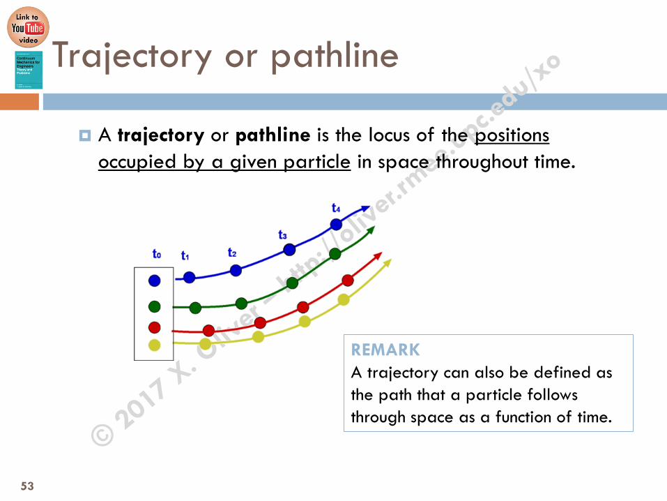
Trajectory or pathline
A trajectory or pathline is the locus of the positions occupied by a given particle in space throughout time.
REMARK A trajectory can also be defined as the path that a particle follows through space as a function of time.
53

Equation of the trajectories
The equation of a given particle’s trajectory is obtained particularizing the equation of motion for that particle, which is identified by it material coordinates X*.
Also, from the velocity field in spatial description, v(x,t): A family of curves is obtained from:
Particularizing for a given particle by imposing the consistency condition inthe reference configuration:
Replacing [2] in [1], the equation of the trajectories in canonical form
( ) ( )( ) ( )
*
*
, ( )
, ( )ii i
t t t
x t t t iϕ φ=
=
= =
= = ∈
X X
X X
x X
X
ϕ φ
( ) ( )( ) ( )1 2 3, , , ], [1d t
t t C C C tdt
= =x
v x x φ
( ) ( ) ( )1 2 30, , , [2]0 i it
t C C C C χ== = =x X X Xφ
( ) ( ) ( )( ) ( )1 2 3, , , ,x X X X XC C C t tφ ϕ= =
54

Example
Consider the following velocity field:
Obtain the equation of the trajectories.
( )
, y
tx
ω = −ω
v x
55

Example - Solution
We integrate the velocity field:
This is a crossed-variable system of differential equations. We derive the 2nd eq. and replace it in the 1st one,
( ) ( )
( ) ( )
( ) ( )
v ,,
v ,
x
y
dx tt yd t dtt
dt dy tt x
dt
= = ω=
= = −ω
xxv x
x
( ) ( ) ( )2
22
d y t dx ty t
dt dt= −ω = −ω 2 0y y′′ + ω =
56

Example - Solution
The characteristic equation:
Has the characteristic solutions:
And the solution of the problem is:
And, using , we obtain
So, the general solution is:
2 2 0r +ω = 1,2jr i j= ± ω ∈
( ) ( )1 2 1 2( ) cos siniwt iwty t Real Part Z e Z e C t C t−= + = ω + ω
dy xdt
= −ω
( ) ( )( )1 21 1 sin cosdyx C t C t
dt= − = − − ω ω + ω ω
ω ω
( ) ( ) ( )( ) ( ) ( )
1 2 1 2
1 2 1 2
, , sin cos
, , cos sin
x C C t C t C t
y C C t C t C t
= ω − ω
= ω + ω
57

Example - Solution
The canonical form is obtained from the initial conditions:
This results in:
( )1 2, ,0C C =x X( ) ( ) ( )
( ) ( ) ( )
1 2 1 2 2
1 2 1 2 1
0 1
1 0
, ,0 sin 0 cos 0
, ,0 cos 0 sin 0
X x C C C C C
Y y C C C C C
= =
= =
= = ω⋅ − ω⋅ = = = ω⋅ + ω⋅ =
( ) ( )( ) ( )
sin cos( , )
cos in
x Y t X tt
y Y t X s t
= ω + ω→ = ω − ω
x X
58
( ) ( ) ( )( ) ( ) ( )
1 2 1 2
1 2 1 2
, , sin cos
, , cos sin
x C C t C t C t
y C C t C t C t
= ω − ω
= ω + ω
Ch.1. Description of Motion
1.8 Streamline
59

Streamline
The streamlines are a family of curves which, for every instant in time, are the velocity field envelopes.
Streamlines are defined for any given time instant and change withthe velocity field.
REMARK The envelopes of vector field are the curves whose tangent vector at each point coincides (in direction and sense but not necessarily in magnitude) with the corresponding vector of the vector field.
time – t0
X
Y
X
Y time – t1
REMARK Two streamlines can never cut each other. Is it true?
60

Equation of the Streamlines
The equation of the streamlines is of the type:
Also, from the velocity field in spatial description, v(x,t*) at a given time instant t*: A family of curves is obtained from:
Where each group identifies a streamline x(λ) whose
points are obtained assigning values to the parameter λ. For each time instant t* a new family of curves is obtained.
( ) ( )( ) ( )1 2 3, * , , , , *d
t C C C tdλ
λ φ λλ
′ ′ ′= =x
v x x
( )v v vx y z
d x d y dz dd dsd
λλ
= = = = =x v
61
( )1 2 3, ,C C C′ ′ ′
vx
v y
vz

Trajectories and Streamlines
For a stationary velocity field, the trajectories and the streamlines coincide – PROOF: 1. If v(x,t)=v(x):
Eq. trajectories:
Eq. streamlines:
The differential equations only differ in the denomination of the integration parameter (t or λ), so the solution to both systems MUST be the same.
( ) ( )( ) ( )1 2 3, , , ,d t
t t C C C tdt
φ= =x
v x x
( ) ( )( ) ( )1 2 3, * , , , , *d
t C C C tdλ
λ φ λλ
= =x
v x x
62
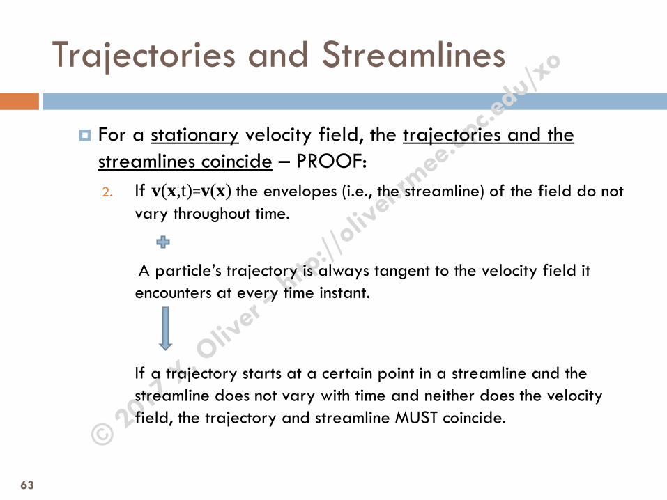
Trajectories and Streamlines
For a stationary velocity field, the trajectories and the streamlines coincide – PROOF: 2. If v(x,t)=v(x) the envelopes (i.e., the streamline) of the field do not
vary throughout time.
A particle’s trajectory is always tangent to the velocity field it
encounters at every time instant. If a trajectory starts at a certain point in a streamline and the
streamline does not vary with time and neither does the velocity field, the trajectory and streamline MUST coincide.
63

Trajectories and Streamlines
The inverse is not necessarily true: if the trajectories and the streamlines coincide, the velocity field is not necessarily stationary – COUNTER-EXAMPLE:
Given the (non-stationary) velocity field:
The eq. trajectory are:
The eq. streamlines are:
( )t 00
at =
v
( )
212
t 00
a t C + =
x
( )1
t 00
at Cλ ′+ =
x
( ) ( )t0 t 00 0
at atd
d dtdt
= =
xx
( ) ( )0 00 0
at atd
d ddλ
λ λλ
= =
xx
64

Example
Consider the following velocity field:
Obtain the equation of the trajectories and the streamlines associated to this vector field.
Do they coincide? Why?
v 1,2,31
ii
x it
= ∈+
65

Example - Solution
Eq. trajectories:
Introducing the velocity field and rearranging:
Integrating both sides of the expression:
The solution:
( ) ( )( )( ) ( )( )
,
v ,ii
d tt t
dtdx t
t t idt
=
= ∈
xv x
x
1i idx x i
dt t= ∈
+
1i
i
dx dt ix t
= ∈+
1 11i
i
dx dtx t
=+∫ ∫ ( ) ( )ln ln 1 ln ln 1i i ix t C C t i= + + = + ∈
( )1i ix C t i= + ∈
66

Example - Solution
Eq. streamlines:
Introducing the velocity field and rearranging:
Integrating both sides of the expression:
The solution:
( ) ( )( )( ) ( )( )*
, *
v ,ii
dt
ddx t
t id
λλ
λ
λλ
=
= ∈
xv x
x
1i idx x i
d tλ= ∈
+
1i
i
dx d ix t
λ= ∈
+
1 11i
i
dx dx t
λ=+∫ ∫ ln
1i ix Kt
λ= +
+
1 1i
ii
Kt tKx e e ei
λ λ
++ + = = ∈
1i i
tx C e iλ
+= ∈
iC=
67

Streamtube
A streamtube is a surface composed of streamlines which pass through the points of a closed contour fixed in space. In stationary cases, the tube will remain fixed in space
throughout time. In non-stationary cases, it will vary (although the closed contour line is fixed).
69
Ch.1. Description of Motion
1.9 Control and Material Surfaces
81

Control Surface
A control surface is a fixed surface in space which does not vary in time.
Mass (particles) can flow across a control surface.
( ) : x , , 0f x y zΣ = =
82

Material Surface
A material surface is a mobile surface in the space constituted always by the same particles. In the reference configuration, the surface Σ0 will be defined in terms
of the material coordinates:
The set of particles (material points)belonging the surface are the same at all times
In spatial description
The set of spatial points belonging to the the surface depends on time The material surface moves in space
( ) 0 : , , 0F X Y ZΣ = =X
( ) : , , , 0t f x y z tΣ = =x
( ) ( ), , ( , ), ( , ), ( , ) ( , ) ( , , , )F X Y Z F X t Y t Z t f t f x y z t= = =x x x x
84

Necessary and sufficient condition for a mobile surface in space, implicitly defined by the function , to be a material surface is that the material derivative of the function is zero: Necessary: if it is a material surface, its material description does not depend
on time:
Sufficient: if the material derivative of f(x,t) is null:
The surface contains always the same set the of particles (it is a material surface)
( ) ( ) ( ) ( ) ( ), ( , ), , 0 , 0Xx x X X xd Ff t f t t F t f td t t
∂→ = = = =
∂
( ) ( ) : , 0 0t f t FΣ = = = =x X Xx
Material Surface
( ), , ,f x y z t
( ) ( ) ( ) ( ) ( , ), ( , ), , 0 , ( , ) ( )Xx x X X x X Xd F tf t f t t F t f t F t Fd t t
∂→ = = = ≡
∂
85
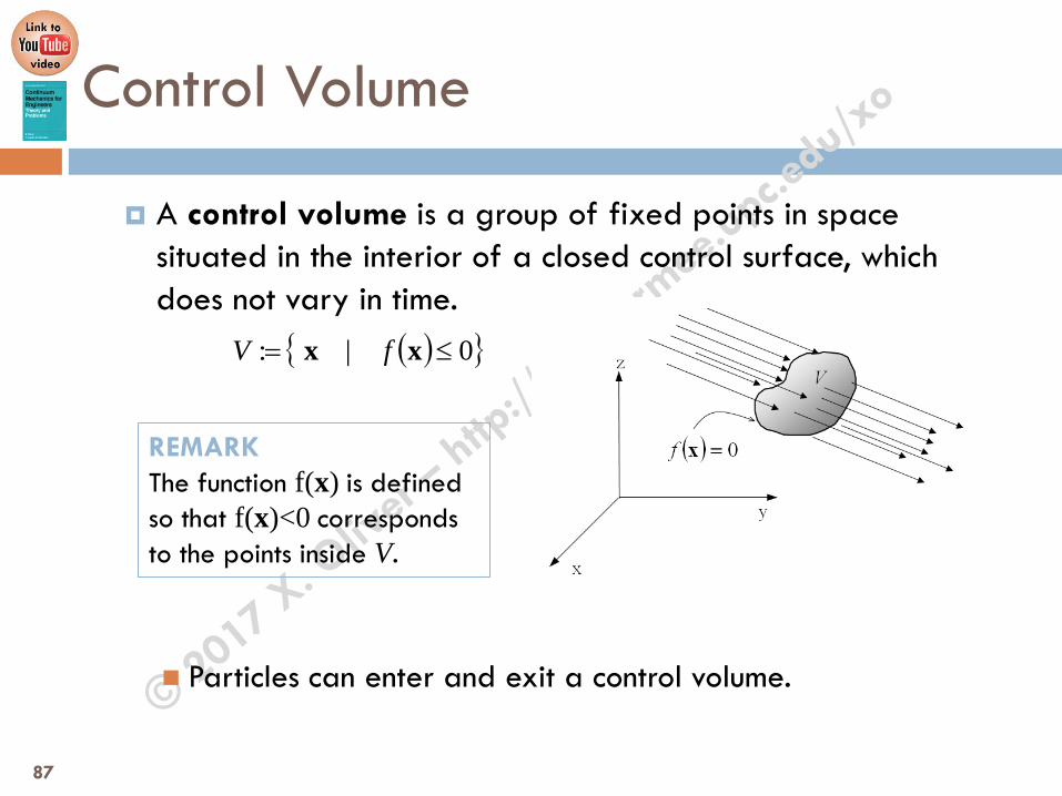
Control Volume
A control volume is a group of fixed points in space situated in the interior of a closed control surface, which does not vary in time.
Particles can enter and exit a control volume.
( ) 0|: ≤= xx fV
REMARK The function f(x) is defined so that f(x)<0 corresponds to the points inside V.
87

Material Volume
A material volume is a (mobile) volume enclosed inside a material boundary or surface. In the reference configuration, the volume V0 will be defined in terms
of the material coordinates:
The particles in the volume are the same at all times
In spatial description, the volume Vt will depend on time.
The set of spatial points belonging to the the volume depends on time The material volume moves in space along time
( ) 0 : | 0V F= ≤X X
( ) : | , 0tV f t= ≤x x
X
89

Material Volume
A material volume is always constituted by the same particles. This is proved by reductio ad absurdum:
If a particle is added into the volume, it would have to cross itsmaterial boundary.
Material boundaries are constituted always by the same particles, so,no particles can cross.
Thus, a material volume is always constituted by the same particles (a material volume is a pack of particles).
90

Contin
uumM
echan
icsfor
Engineer
s
Theory
and Pro
blems
©X. O
liver
and C. A
gelet
de Sarac
ibar
Chapter 1Description of Motion
1.1 Definition of the Continuous MediumA continuous medium is understood as an infinite set of particles (which formpart of, for example, solids or fluids) that will be studied macroscopically, thatis, without considering the possible discontinuities existing at microscopic level(atomic or molecular level). Accordingly, one admits that there are no discon-tinuities between the particles and that the mathematical description of thismedium and its properties can be described by continuous functions.
1.2 Equations of MotionThe most basic description of the motion of a continuous medium can beachieved by means of mathematical functions that describe the position of eachparticle along time. In general, these functions and their derivatives are requiredto be continuous.
Definition 1.1. Consider the following definitions:
• Spatial point: Fixed point in space.
• Material point: A particle. It may occupy different spatial pointsduring its motion along time.
• Configuration: Locus of the positions occupied in space by theparticles of the continuous medium at a given time t.
The continuous medium is assumed to be composed of an infinite number ofparticles (material points) that occupy different positions in the physical spaceduring its motion along time (see Figure 1.1). The configuration of the contin-
1

Contin
uumM
echan
icsfor
Engineer
s
Theory
and Pro
blems
©X. O
liver
and C. A
gelet
de Sarac
ibar
2 CHAPTER 1. DESCRIPTION OF MOTION
Ω0 – reference configuration
t0 – reference time
Ωt – present configuration
t – present time
Figure 1.1: Configurations of the continuous medium.
uous medium at time t, denoted by Ωt , is defined as the locus of the positionsoccupied in space by the material points (particles) of the continuous medium atthe given time.
A certain time t = t0 of the time interval of interest is referred to as the ref-erence time and the configuration at this time, denoted by Ω0, is referred to asinitial, material or reference configuration1.
Consider now the Cartesian coordinate system (X ,Y,Z) in Figure 1.1 and thecorresponding orthonormal basis e1, e2, e3. In the reference configuration Ω0,the position vector X of a particle occupying a point P in space (at the referencetime) is given by2,3
X = X1e1 +X2e2 +X3e3 = Xiei, (1.1)
where the components (X1,X2,X3) are referred to as material coordinates (of the
particle) and can be collected in a vector of components denoted as4
X not≡ [X] =
⎡⎢⎣X1
X2
X3
⎤⎥⎦ de f
= material coordinates. (1.2)
1 In general, the time t0 = 0 will be taken as the reference time.2 Notations (X ,Y,Z) and (X1,X2,X3) will be used indistinctly to designate the Cartesiancoordinate system.3 Einstein or repeated index notation will be used in the remainder of this text. Every repe-tition of an index in the same monomial of an algebraic expression represents the sum overthat index. For example,
i=3
∑i=1
Xieinot= Xiei ,
k=3
∑k=1
aikbk jnot= aikbk j and
i=3
∑i=1
j=3
∑j=1
ai jbi jnot= ai jbi j.
4 Here, the vector (physical entity) X is distinguished from its vector of components [X].Henceforth, the symbol
not≡ (equivalent notation) will be used to indicate that the tensor andcomponent notations at either side of the symbol are equivalent when the system of coordi-nates used remains unchanged.
X. Oliver and C. Agelet de Saracibar Continuum Mechanics for Engineers.Theory and Problems
doi:10.13140/RG.2.2.25821.20961

Contin
uumM
echan
icsfor
Engineer
s
Theory
and Pro
blems
©X. O
liver
and C. A
gelet
de Sarac
ibar
Equations of Motion 3
In the present configuration Ωt5, a particle originally located at a material
point P (see Figure 1.1) occupies a spatial point P′ and its position vector x isgiven by
x = x1e1 + x2e2 + x3e3 = xiei, (1.3)
where (x1,x2,x3) are referred to as spatial coordinates of the particle at time t,
x not≡ [x] =
⎡⎢⎣ x1
x2
x3
⎤⎥⎦ de f
= spatial coordinates. (1.4)
The motion of the particles of the continuous medium can now be describedby the evolution of their spatial coordinates (or their position vector) along time.Mathematically, this requires the definition of a function that provides for eachparticle (identified by its label) its spatial coordinates xi (or its spatial positionvector x) at successive instants of time. The material coordinates Xi of the par-ticle can be chosen as the label that univocally characterizes it and, thus, theequation of motion
x = ϕ (particle, t) = ϕ (X, t) not= x(X, t)
xi = ϕi (X1,X2,X3, t) i ∈ 1,2,3(1.5)
is obtained, which provides the spatial coordinates in terms of the material ones.The spatial coordinates xi of the particle can also be chosen as label, definingthe inverse equation of motion6 as
X = ϕ−1 (x, t) not= X(x, t) ,
Xi = ϕ−1i (x1,x2,x3, t) i ∈ 1,2,3 ,
(1.6)
which provides the material coordinates in terms of the spatial ones.
Remark 1.1. There are different alternatives when choosing the la-bel that characterizes a particle, even though the option of using itsmaterial coordinates is the most common one. When the equation ofmotion is written in terms of the material coordinates as label (as in(1.5)), one refers to it as the equation of motion in canonical form.
5 Whenever possible, uppercase letters will be used to denote variables relating to the refer-ence configuration Ω0 and lowercase letters to denote the variables referring to the currentconfiguration Ωt .6 With certain abuse of notation, the function will be frequently confused with its image.Hence, the equation of motion will be often written as x = x(X, t) and its inverse equation asX = X(x, t).
X. Oliver and C. Agelet de Saracibar Continuum Mechanics for Engineers.Theory and Problems
doi:10.13140/RG.2.2.25821.20961

Contin
uumM
echan
icsfor
Engineer
s
Theory
and Pro
blems
©X. O
liver
and C. A
gelet
de Sarac
ibar
4 CHAPTER 1. DESCRIPTION OF MOTION
There exist certain mathematical restrictions to guarantee the existence of ϕand ϕ−1, as well as their correct physical meaning. These restrictions are:
• ϕ (X,0) = X since, by definition, X is the position vector at the referencetime t = 0 (consistency condition).
• ϕ ∈ C1 (function ϕ is continuous with continuous derivatives at each pointand at each instant of time).
• ϕ is biunivocal (to guarantee that two particles do not occupy simultaneouslythe same point in space and that a particle does not occupy simultaneouslymore than one point in space).
• The Jacobian of the transformation J = det
[∂ϕ (X, t)
∂X
]not=
∣∣∣∣∂ϕ (X, t)∂X
∣∣∣∣> 0.
The physical interpretation of this condition (which will be studied later) isthat every differential volume must always be positive or, using the principle ofmass conservation (which will be seen later), the density of the particles mustalways be positive.
Remark 1.2. The equation of motion at the reference time t = 0 re-sults in x(X, t)|t=0 = X. Accordingly, x = X , y = Y , z = Z is theequation of motion at the reference time and the Jacobian at this in-stant of time is7
J (X,0) =
∣∣∣∣ ∂ (xyz)∂ (XY Z)
∣∣∣∣= det
[∂xi
∂Xj
]= det [δi j] = det1 = 1.
Figure 1.2: Trajectory or pathline of a particle.
7 The two-index operator Delta Kroneckernot= δi j is defined as δi j = 0 when i = j and δi j = 1
when i = j. Then, the unit tensor 1 is defined as [1]i j = δi j.
X. Oliver and C. Agelet de Saracibar Continuum Mechanics for Engineers.Theory and Problems
doi:10.13140/RG.2.2.25821.20961
Contin
uumM
echan
icsfor
Engineer
s
Theory
and Pro
blems
©X. O
liver
and C. A
gelet
de Sarac
ibar
Equations of Motion 5
Remark 1.3. The expression x = ϕ (X, t), particularized for a fixedvalue of the material coordinates X, provides the equation of thetrajectory or pathline of a particle (see Figure 1.2).
Example 1.1 – The spatial description of the motion of a continuous mediumis given by
x(X, t) not≡
⎡⎢⎣ x1 = X1e2t
x2 = X2e−2t
x3 = 5X1t +X3e2t
⎤⎥⎦=
⎡⎢⎣ x = Xe2t
y = Y e−2t
z = 5Xt +Ze2t
⎤⎥⎦
Obtain the inverse equation of motion.
Solution
The determinant of the Jacobian is computed as
J =
∣∣∣∣ ∂xi
∂Xj
∣∣∣∣=
∣∣∣∣∣∣∣∣∣∣∣∣∣∣
∂x1
∂X1
∂x1
∂X2
∂x1
∂X3
∂x2
∂X1
∂x2
∂X2
∂x2
∂X3
∂x3
∂X1
∂x3
∂X2
∂x3
∂X3
∣∣∣∣∣∣∣∣∣∣∣∣∣∣=
∣∣∣∣∣∣∣∣e2t 0 0
0 e−2t 0
5t 0 e2t
∣∣∣∣∣∣∣∣= e2t = 0.
The sufficient (but not necessary) condition for the function x = ϕ (X, t) tobe biunivocal (that is, for its inverse to exist) is that the determinant of theJacobian of the function is not null. In addition, since the Jacobian is positive,the motion has physical sense. Therefore, the inverse of the given spatialdescription exists and is determined by
X = ϕ−1 (x, t) not≡
⎡⎢⎢⎣
X1
X2
X3
⎤⎥⎥⎦=
⎡⎢⎢⎣
x1e−2t
x2e2t
x3e−2t −5tx1e−4t
⎤⎥⎥⎦ .
X. Oliver and C. Agelet de Saracibar Continuum Mechanics for Engineers.Theory and Problems
doi:10.13140/RG.2.2.25821.20961
Contin
uumM
echan
icsfor
Engineer
s
Theory
and Pro
blems
©X. O
liver
and C. A
gelet
de Sarac
ibar
6 CHAPTER 1. DESCRIPTION OF MOTION
1.3 Descriptions of MotionThe mathematical description of the properties of the particles of the continu-ous medium can be addressed in two alternative ways: the material description(typically used in solid mechanics) and the spatial description (typically usedin fluid mechanics). Both descriptions essentially differ in the type of argument(material coordinates or spatial coordinates) that appears in the mathematicalfunctions that describe the properties of the continuous medium.
1.3.1 Material DescriptionIn the material description8, a given property (for example, the density ρ) isdescribed by a certain function ρ (•, t) : R3×R+ → R+, where the argument (•)in ρ (•, t) represents the material coordinates,
ρ = ρ (X, t) = ρ (X1,X2,X3, t) . (1.7)
Here, if the three arguments X≡ (X1,X2,X3) are fixed, a specific particle is beingfollowed (see Figure 1.3) and, hence, the name of material description.
1.3.2 Spatial DescriptionIn the spatial description9, the focus is on a point in space. The property is de-scribed as a function ρ (•, t) : R3 ×R+ → R+ of the point in space and of time,
ρ = ρ (x, t) = ρ (x1,x2,x3, t) . (1.8)
Then, when the argument x in ρ = ρ (x, t) is assigned a certain value, the evolu-tion of the density for the different particles that occupy the point in space alongtime is obtained (see Figure 1.3). Conversely, fixing the time argument in (1.8)results in an instantaneous distribution (like a snapshot) of the property in space.Obviously, the direct and inverse equations of motion allow shifting from one
Figure 1.3: Material description (left) and spatial description (right) of a property.
8 Literature on this topic also refers to the material description as Lagrangian description.9 The spatial description is also referred to as Eulerian description.
X. Oliver and C. Agelet de Saracibar Continuum Mechanics for Engineers.Theory and Problems
doi:10.13140/RG.2.2.25821.20961

Contin
uumM
echan
icsfor
Engineer
s
Theory
and Pro
blems
©X. O
liver
and C. A
gelet
de Sarac
ibar
Descriptions of Motion 7
description to the other as follows.ρ (x, t) = ρ (x(X, t) , t) = ρ (X, t)
ρ (X, t) = ρ (X(x, t) , t) = ρ (x, t)(1.9)
Example 1.2 – The equation of motion of a continuous medium is
x = x(X, t) not≡[ x = X −Yt
y = Xt +Yz =−Xt +Z
].
Obtain the spatial description of the property whose material description is
ρ (X ,Y,Z, t) =X +Y +Z
1+ t2.
Solution
The equation of motion is given in the canonical form since in the referenceconfiguration Ω0 its expression results in
x = X(X,0)not≡
[ x = Xy = Yz = Z
].
The determinant of the Jacobian is
J =
∣∣∣∣ ∂xi
∂Xj
∣∣∣∣=
∣∣∣∣∣∣∣∣∣∣∣∣∣
∂x∂X
∂x∂Y
∂x∂Z
∂y∂X
∂y∂Y
∂y∂Z
∂ z∂X
∂ z∂Y
∂ z∂Z
∣∣∣∣∣∣∣∣∣∣∣∣∣=
∣∣∣∣∣∣∣∣1 −t 0
t 1 0
−t 0 1
∣∣∣∣∣∣∣∣= 1+ t2 = 0
and the inverse equation of motion is given by
X(x, t) not≡
⎡⎢⎢⎢⎢⎢⎢⎢⎣
X =x+ yt1+ t2
Y =y− xt1+ t2
Z =z+ zt2 + xt + yt2
1+ t2
⎤⎥⎥⎥⎥⎥⎥⎥⎦.
X. Oliver and C. Agelet de Saracibar Continuum Mechanics for Engineers.Theory and Problems
doi:10.13140/RG.2.2.25821.20961
Contin
uumM
echan
icsfor
Engineer
s
Theory
and Pro
blems
©X. O
liver
and C. A
gelet
de Sarac
ibar
8 CHAPTER 1. DESCRIPTION OF MOTION
Consider now the material description of the property,
ρ (X ,Y,Z, t) =X +Y +Z
1+ t2,
its spatial description is obtained by introducing the inverse equation of mo-tion into the expression above,
ρ (X ,Y,Z, t)≡ x+ yt + y+ z+ zt2 + yt2
(1+ t2)2= ρ (x,y,z, t) .
1.4 Time Derivatives: Local, Material and ConvectiveThe consideration of different descriptions (material and spatial) of the proper-ties of the continuous medium leads to diverse definitions of the time derivativesof these properties. Consider a certain property and its material and spatial de-scriptions,
Γ (X, t) = γ (x, t) , (1.10)
in which the change from the spatial to the material description and vice versais performed by means of the equation of motion (1.5) and its inverse equa-tion (1.6).
Definition 1.2. The local derivative of a property is its variationalong time at a fixed point in space. If the spatial description γ (x, t)of the property is available, the local derivative is mathematicallywritten as10
local derivativenot=
∂γ (x, t)∂ t
.
The material derivative of a property is its variation along time fol-lowing a specific particle (material point) of the continuous medium.If the material description Γ (X, t) of the property is available, thematerial derivative is mathematically written as
material derivativenot=
ddt
Γ =∂Γ (X, t)
∂ t.
10 The expression ∂ (•, t)/∂ t is understood in the classical sense of partial derivative withrespect to the variable t.
X. Oliver and C. Agelet de Saracibar Continuum Mechanics for Engineers.Theory and Problems
doi:10.13140/RG.2.2.25821.20961

Contin
uumM
echan
icsfor
Engineer
s
Theory
and Pro
blems
©X. O
liver
and C. A
gelet
de Sarac
ibar
Time Derivatives: Local, Material and Convective 9
However, taking the spatial description of the property γ (x, t) and consideringthe equation of motion is implicit in this expression yields
γ (x, t) = γ (x(X, t) , t) = Γ (X, t) . (1.11)
Then, the material derivative (following a particle) is obtained from the spatialdescription of the property as
material derivativenot=
ddt
γ (x(X, t) , t) =∂Γ (X, t)
∂ t. (1.12)
Expanding (1.12) results in11
dγ (x(X, t) , t)dt
=∂γ (x, t)
∂ t+
∂γ∂xi
∂xi
∂ t=
∂γ (x, t)∂ t
+∂γ∂x
· ∂x∂ t︸︷︷︸
v(x, t)
=
=∂γ (x, t)
∂ t+
∂γ∂x
·v(x, t) ,(1.13)
where the definition of velocity as the derivative of the equation of motion (1.5)with respect to time has been taken into account,
∂x(X, t)∂ t
= V(X(x, t) , t) = v(x, t) . (1.14)
The deduction of the material derivative from the spatial description can begeneralized for any property χ (x, t) (of scalar, vectorial or tensorial character)
as12
dχ (x, t)dt︸ ︷︷ ︸
materialderivative
=∂ χ (x, t)
∂ t︸ ︷︷ ︸local
derivative
+ v(x, t) ·∇χ (x, t)︸ ︷︷ ︸convectivederivative
. (1.15)
Remark 1.4. The expression in (1.15) implicitly defines the convec-tive derivative v ·∇(•) as the difference between the material andspatial derivatives of the property. In continuum mechanics, the termconvection is applied to phenomena that are related to mass (or par-ticle) transport. Note that, if there is no convection (v = 0), the con-vective derivative disappears and the local and material derivativescoincide.
11 In literature, the notation D(•)/Dt is often used as an alternative to d(•)/dt.12 The symbolic form of the spatial Nabla operator, ∇ ≡ ∂ ei/∂xi , is considered here.
X. Oliver and C. Agelet de Saracibar Continuum Mechanics for Engineers.Theory and Problems
doi:10.13140/RG.2.2.25821.20961
Contin
uumM
echan
icsfor
Engineer
s
Theory
and Pro
blems
©X. O
liver
and C. A
gelet
de Sarac
ibar
10 CHAPTER 1. DESCRIPTION OF MOTION
Example 1.3 – Given the equation of motion
x(X, t) not≡[ x = X +Yt +Zt
y = Y +2Ztz = Z +3Xt
],
and the spatial description of a property, ρ (x, t) = 3x+ 2y+ 3t, obtain thematerial derivative of this property.
Solution
The material description of the property is obtained introducing the equationof motion into its spatial description,
ρ (X ,Y,Z, t)= 3(X +Yt +Zt)+2(Y +2Zt)+3t = 3X+3Yt+7Zt+2Y +3t .
The material derivative is then calculated as the derivative of the materialdescription with respect to time,
∂ρ∂ t
= 3Y +7Z +3 .
An alternative way of deducing the material derivative is by using the conceptof material derivative of the spatial description of the property,
dρdt
=∂ρ∂ t
+v ·∇ρ with
∂ρ∂ t
= 3 , v =∂x∂ t
= [Y +Z, 2Z, 3X ]T and ∇ρ = [3, 2, 0]T .
Replacing in the expression of the material derivative operator,
dρdt
= 3+3Y +7Z
is obtained. Note that the expressions for the material derivative obtainedfrom the material description, ∂ρ/∂ t, and the spatial description, dρ/dt, co-incide.
X. Oliver and C. Agelet de Saracibar Continuum Mechanics for Engineers.Theory and Problems
doi:10.13140/RG.2.2.25821.20961

Contin
uumM
echan
icsfor
Engineer
s
Theory
and Pro
blems
©X. O
liver
and C. A
gelet
de Sarac
ibar
Velocity and Acceleration 11
1.5 Velocity and Acceleration
Definition 1.3. The velocity is the time derivative of the equation ofmotion.
The material description of velocity is, consequently, given by⎧⎪⎪⎨⎪⎪⎩
V(X, t) =∂x(X, t)
∂ t
Vi (X, t) =∂xi (X, t)
∂ ti ∈ 1, 2, 3
(1.16)
and, if the inverse equation of motion X = ϕ−1 (x, t) is known, the spatial de-scription of the velocity can be obtained as
v(x, t) = V(X(x, t) , t) . (1.17)
Definition 1.4. The acceleration is the time derivative of the velocityfield.
If the velocity is described in material form, the material description of theacceleration is given by⎧⎪⎪⎨
⎪⎪⎩A(X, t) =
∂V(X, t)∂ t
Ai (X, t) =∂Vi (X, t)
∂ ti ∈ 1, 2, 3
(1.18)
and, through the inverse equation of motion X = ϕ−1 (x, t), the spatial descrip-tion is obtained, a(x, t) = A(X(x, t) , t). Alternatively, if the spatial descriptionof the velocity is available, applying (1.15) to obtain the material derivative ofv(x, t),
a(x, t) =dv(x, t)
dt=
∂v(x, t)∂ t
+v(x, t) ·∇v(x, t) , (1.19)
directly yields the spatial description of the acceleration.
X. Oliver and C. Agelet de Saracibar Continuum Mechanics for Engineers.Theory and Problems
doi:10.13140/RG.2.2.25821.20961

Contin
uumM
echan
icsfor
Engineer
s
Theory
and Pro
blems
©X. O
liver
and C. A
gelet
de Sarac
ibar
12 CHAPTER 1. DESCRIPTION OF MOTION
Example 1.4 – Consider the solid in the figure below, which rotates at aconstant angular velocity ω and has the expression
x = Rsin(ωt +φ)
y = Rcos(ωt +φ)
as its equation of motion. Find the velocity and acceleration of the motiondescribed both in material and spatial forms.
Solution
The equation of motion can be rewritten asx = Rsin(ωt +φ) = Rsin(ωt)cosφ +Rcos(ωt)sinφy = Rcos(ωt +φ) = Rcos(ωt)cosφ −Rsin(ωt)sinφ
and, since for t = 0, X = Rsinφ and Y = Rcosφ , the canonical form of theequation of motion and its inverse equation result in
x = X cos(ωt)+Y sin(ωt)
y =−X sin(ωt)+Y cos(ωt)and
X = xcos(ωt)− ysin(ωt)
Y = xsin(ωt)+ ycos(ωt).
Velocity in material description:
V(X, t) =∂x(X, t)
∂ t)
not≡
⎡⎢⎢⎣
∂x∂ t
=−Xω sin(ωt)+Y ω cos(ωt)
∂y∂ t
=−Xω cos(ωt)−Y ω sin(ωt)
⎤⎥⎥⎦
Velocity in spatial description:Replacing the canonical form of the equation of motion into the materialdescription of the velocity results in
v(x, t) = V(X(x, t) , t) not≡[
ωy−ωx
].
X. Oliver and C. Agelet de Saracibar Continuum Mechanics for Engineers.Theory and Problems
doi:10.13140/RG.2.2.25821.20961

Contin
uumM
echan
icsfor
Engineer
s
Theory
and Pro
blems
©X. O
liver
and C. A
gelet
de Sarac
ibar
Velocity and Acceleration 13
Acceleration in material description:
A(X, t) =∂V(X, t)
∂ t
A(X, t) not≡
⎡⎢⎢⎢⎣
∂vx
∂ t=−Xω2 cos(ωt)−Y ω2 sin(ωt)
∂vy
∂ t= Xω2 sin(ωt)−Y ω2 cos(ωt)
⎤⎥⎥⎥⎦=
=−ω2
[X cos(ωt)+Y sin(ωt)
−X sin(ωt)+Y cos(ωt)
]
Acceleration in spatial description:Replacing the canonical form of the equation of motion into the materialdescription of the acceleration results in
a(x, t) = A(X(x, t) , t) not≡[−ω2x
−ω2y
].
This same expression can be obtained if the expression for the velocity v(x, t)and the definition of material derivative in (1.15) are taken into account,
a(x, t) =dv(x, t)
dt=
∂v(x, t)∂ t
+v(x, t) ·∇v(x, t) =
not≡ ∂∂ t
[ωy−ωx
]+[
ωy , −ωx]⎡⎢⎢⎢⎣
∂∂x∂∂y
⎤⎥⎥⎥⎦[
ωy , −ωx],
a(x, t) not≡[
0
0
]+[
ωy , −ωx]⎡⎢⎢⎢⎣
∂∂x
(ωy)∂∂x
(−ωx)
∂∂y
(ωy)∂∂y
(−ωx)
⎤⎥⎥⎥⎦=
[−ω2x
−ω2y
].
Note that the result obtained using both procedures is identical.
X. Oliver and C. Agelet de Saracibar Continuum Mechanics for Engineers.Theory and Problems
doi:10.13140/RG.2.2.25821.20961

Contin
uumM
echan
icsfor
Engineer
s
Theory
and Pro
blems
©X. O
liver
and C. A
gelet
de Sarac
ibar
14 CHAPTER 1. DESCRIPTION OF MOTION
1.6 Stationarity
Definition 1.5. A property is stationary when its spatial descriptiondoes not depend on time.
According to the above definition, and considering the concept of local deriva-tive, any stationary property has a null local derivative. For example, if the ve-locity for a certain motion is stationary, it can be described in spatial form as
v(x, t) = v(x) ⇐⇒ ∂v(x, t)∂ t
= 0 . (1.20)
Remark 1.5. The non-dependence on time of the spatial description(stationarity) assumes that, for a same point in space, the propertybeing considered does not vary along time. This does not imply that,for a same particle, such property does not vary along time (the ma-terial description may depend on time). For example, if the velocityv(x, t) is stationary,
v(x, t)≡ v(x) = v(x(X, t)) = V(X, t) ,
and, thus, the material description of the velocity depends on time.In the case of stationary density (see Figure 1.4), for two particleslabeled X1 and X2 that have varying densities along time, when oc-cupying a same spatial point x (at two different times t1 and t2) theirdensity value will coincide,
ρ (X1, t1) = ρ (X2, t2) = ρ (x) .
That is, for an observer placed outside the medium, the density ofthe fixed point in space x will always be the same.
Figure 1.4: Motion of two particles with stationary density.
X. Oliver and C. Agelet de Saracibar Continuum Mechanics for Engineers.Theory and Problems
doi:10.13140/RG.2.2.25821.20961
Contin
uumM
echan
icsfor
Engineer
s
Theory
and Pro
blems
©X. O
liver
and C. A
gelet
de Sarac
ibar
Trajectory 15
Example 1.5 – Justify if the motion described in Example 1.4 is stationaryor not.
Solution
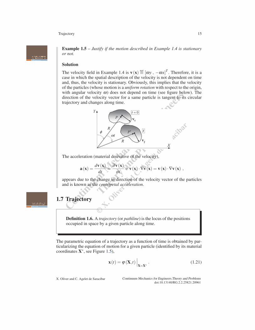
The velocity field in Example 1.4 is v(x) not≡ [ωy , −ωx]T . Therefore, it is acase in which the spatial description of the velocity is not dependent on timeand, thus, the velocity is stationary. Obviously, this implies that the velocityof the particles (whose motion is a uniform rotation with respect to the origin,with angular velocity ω) does not depend on time (see figure below). Thedirection of the velocity vector for a same particle is tangent to its circulartrajectory and changes along time.
The acceleration (material derivative of the velocity),
a(x) =dv(x)
dt=
∂v(x)∂ t
+v(x) ·∇v(x) = v(x) ·∇v(x) ,
appears due to the change in direction of the velocity vector of the particlesand is known as the centripetal acceleration.
1.7 Trajectory
Definition 1.6. A trajectory (or pathline) is the locus of the positionsoccupied in space by a given particle along time.
The parametric equation of a trajectory as a function of time is obtained by par-ticularizing the equation of motion for a given particle (identified by its materialcoordinates X∗, see Figure 1.5),
x(t) = ϕ (X, t)∣∣∣X=X∗ . (1.21)
X. Oliver and C. Agelet de Saracibar Continuum Mechanics for Engineers.Theory and Problems
doi:10.13140/RG.2.2.25821.20961

Contin
uumM
echan
icsfor
Engineer
s
Theory
and Pro
blems
©X. O
liver
and C. A
gelet
de Sarac
ibar
16 CHAPTER 1. DESCRIPTION OF MOTION
Figure 1.5: Trajectory or pathline of a particle.
Given the equation of motion x = ϕ (X, t), each point in space is occupiedby a trajectory characterized by the value of the label (material coordinates) X.Then, the equation of motion defines a family of curves whose elements are thetrajectories of the various particles.
1.7.1 Differential Equation of the TrajectoriesGiven the velocity field in spatial description v(x, t), the family of trajectoriescan be obtained by formulating the system of differential equations that imposesthat, for each point in space x, the velocity vector is the time derivative of theparametric equation of the trajectory defined in (1.21), i.e.,
Find x(t) :=
⎧⎪⎪⎨⎪⎪⎩
dx(t)dt
= v(x(t) , t) ,
dxi (t)dt
= vi (x(t) , t) i ∈ 1, 2, 3 .
(1.22)
The solution to this first-order system of differential equations depends on threeintegration constants (C1,C2,C3),
x = φ (C1,C2,C3, t) ,
x = φi (C1,C2,C3, t) i ∈ 1, 2, 3 .(1.23)
These expressions constitute a family of curves in space parametrized by theconstants (C1,C2,C3). Assigning a particular value to these constants yields amember of the family, which is the trajectory of a particle characterized by thelabel (C1,C2,C3).
To obtain the equation in canonical form, the consistency condition is im-posed in the reference configuration,
x(t)∣∣∣t=0=X =⇒ X= φ (C1,C2,C3,0) =⇒ Ci = χi (X) i∈ 1, 2, 3 , (1.24)
and, replacing into (1.23), the canonical form of the equation of the trajectory,
X = φ (C1 (X) ,C2 (X) ,C3 (X) , t) = ϕ (X, t) , (1.25)
is obtained.
X. Oliver and C. Agelet de Saracibar Continuum Mechanics for Engineers.Theory and Problems
doi:10.13140/RG.2.2.25821.20961

Contin
uumM
echan
icsfor
Engineer
s
Theory
and Pro
blems
©X. O
liver
and C. A
gelet
de Sarac
ibar
Trajectory 17
Example 1.6 – Given the velocity field in Example 1.5, v(x) not≡ [ωy , −ωx]T ,obtain the equation of the trajectory.
Solution
Using expression (1.22), one can write
dx(t)dt
= v(x, t) =⇒
⎧⎪⎪⎨⎪⎪⎩
dx(t)dt
= vx (x, t) = ωy ,
dy(t)dt
= vy (x, t) =−ωx .
This system of equations is a system with crossed variables. Differentiatingthe second equation and replacing the result obtained into the first equationyields
d2y(t)dt2
=−ωdx(t)
dt=−ω2y(t) =⇒ y′′+ω2y = 0 .
The characteristic equation of this second-order differential equation isr2 +ω2 = 0 and its characteristic solutions are r j = ±iω j ∈ 1, 2.Therefore, the y component of the equation of the trajectory is
y(t) = Real Part
C1eiwt +C2e−iwt=C1 cos(ωt)+C2 sin(ωt) .
The solution for x(t) is obtained from dy/dt = −ωx , which results inx =−dy/(ω dt) and, therefore,
x(C1,C2, t) =C1 sin(ωt)−C2 cos(ωt) ,
y(C1,C2, t) =C1 cos(ωt)+C2 sin(ωt) .
This equation provides the expressions of the trajectories in a non-canonicalform. The canonical form is obtained considering the initial condition,
x(C1,C2,0) = X ,
that is, x(C1,C2,0) =−C2 = X ,
y(C1,C2,0) =C1 = Y .
Finally, the equation of motion, or the equation of the trajectory, in canonicalform
x = Y sin(ωt)+X cos(ωt)
y = Y cos(ωt)−X sin(ωt)
is obtained.
X. Oliver and C. Agelet de Saracibar Continuum Mechanics for Engineers.Theory and Problems
doi:10.13140/RG.2.2.25821.20961
Contin
uumM
echan
icsfor
Engineer
s
Theory
and Pro
blems
©X. O
liver
and C. A
gelet
de Sarac
ibar
18 CHAPTER 1. DESCRIPTION OF MOTION
1.8 Streamline
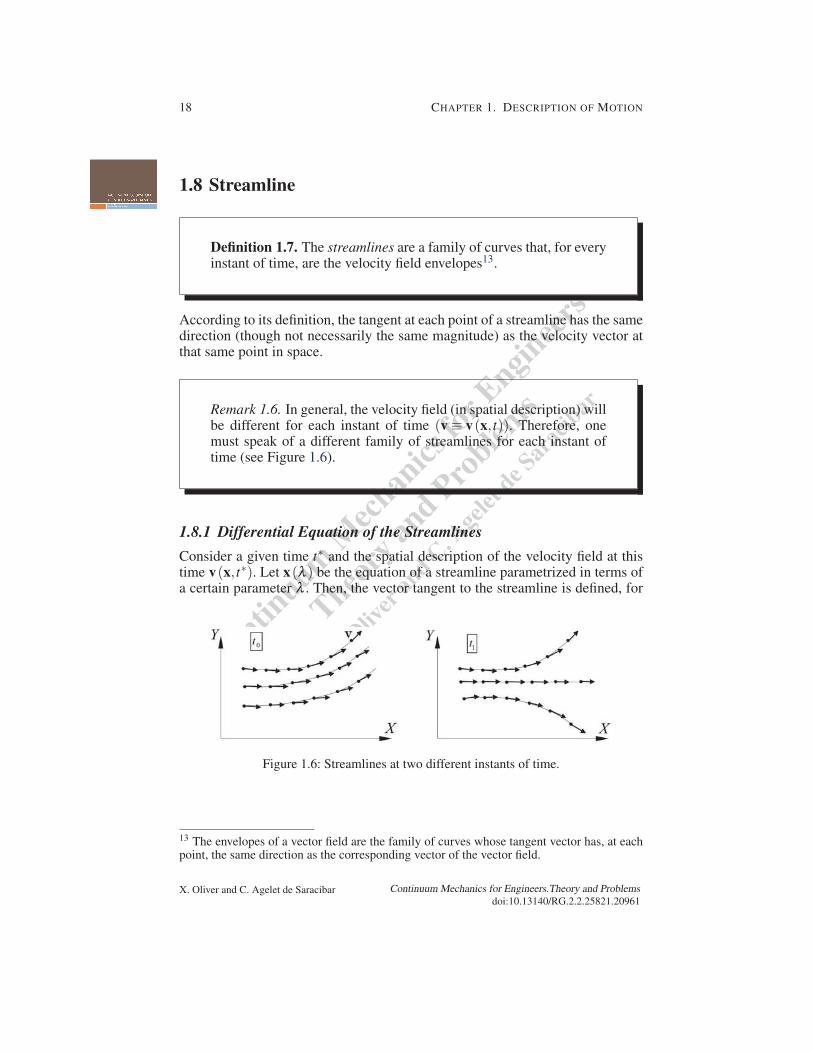
Definition 1.7. The streamlines are a family of curves that, for everyinstant of time, are the velocity field envelopes13.
According to its definition, the tangent at each point of a streamline has the samedirection (though not necessarily the same magnitude) as the velocity vector atthat same point in space.
Remark 1.6. In general, the velocity field (in spatial description) willbe different for each instant of time (v ≡ v(x, t)). Therefore, onemust speak of a different family of streamlines for each instant oftime (see Figure 1.6).
1.8.1 Differential Equation of the StreamlinesConsider a given time t∗ and the spatial description of the velocity field at thistime v(x, t∗). Let x(λ ) be the equation of a streamline parametrized in terms ofa certain parameter λ . Then, the vector tangent to the streamline is defined, for
Figure 1.6: Streamlines at two different instants of time.
13 The envelopes of a vector field are the family of curves whose tangent vector has, at eachpoint, the same direction as the corresponding vector of the vector field.
X. Oliver and C. Agelet de Saracibar Continuum Mechanics for Engineers.Theory and Problems
doi:10.13140/RG.2.2.25821.20961

Contin
uumM
echan
icsfor
Engineer
s
Theory
and Pro
blems
©X. O
liver
and C. A
gelet
de Sarac
ibar
Streamline 19
each value of λ 14, by dx(λ )/dλ and the vector field tangency condition can bewritten as follows.
Find x(λ ) :=
⎧⎪⎪⎨⎪⎪⎩
dx(λ )dλ
= v(x(λ ) , t∗) ,
dxi (λ )dλ
= vi (x(λ ) , t∗) i ∈ 1, 2, 3 .(1.26)
The expressions in (1.26) constitute a system of first-order differential equa-tions whose solution for each time t∗, which will depend on three integrationconstants (C′
1,C′2,C
′3), provides the parametric expression of the streamlines,x = φ (C′
1,C′2,C
′3,λ , t∗) ,
xi = φi (C′1,C
′2,C
′3,λ , t∗) i ∈ 1, 2, 3 .
(1.27)
Each triplet of integration constants (C′1,C
′2,C
′3) identifies a streamline whose
points, in turn, are obtained by assigning values to the parameter λ . For eachtime t∗ a new family of streamlines is obtained.
Remark 1.7. In a stationary velocity field (v(x, t)≡ v(x)) the trajec-tories and streamlines coincide. This can be proven from two differ-ent viewpoints:
• The fact that the time variable does not appear in (1.22) or (1.26)means that the differential equations defining the trajectories andthose defining the streamlines only differ in the denomination ofthe integration parameter (t or λ , respectively). The solution toboth systems must be, therefore, the same, except for the nameof the parameter used in each type of curves.
• From a more physical point of view: a) If the velocity field isstationary, its envelopes (the streamlines) do not change alongtime; b) a given particle moves in space keeping the trajectoryin the direction tangent to the velocity field it encounters alongtime; c) consequently, if a trajectory starts at a certain point in astreamline, it will stay on this streamline throughout time.
14 It is assumed that the value of the parameter λ is chosen such that, at each point in spacex, not only does dx(λ )/dλ have the same direction as the vector v(x, t), but it coincidestherewith.
X. Oliver and C. Agelet de Saracibar Continuum Mechanics for Engineers.Theory and Problems
doi:10.13140/RG.2.2.25821.20961

Contin
uumM
echan
icsfor
Engineer
s
Theory
and Pro
blems
©X. O
liver
and C. A
gelet
de Sarac
ibar
20 CHAPTER 1. DESCRIPTION OF MOTION
1.9 Streamtubes
Definition 1.8. A streamtube is a surface formed by a bundle ofstreamlines that occupy the points of a closed line, fixed in space,and that does not constitute a streamline.
In non-stationary cases, even though the closed line does not vary in space, thestreamtube and streamlines do change. On the contrary, in a stationary case, thestreamtube remains fixed in space along time.
1.9.1 Equation of the StreamtubeStreamlines constitute a family of curves of the type
x = f(C1,C2,C3,λ , t) . (1.28)
The problem consists in determining, for each instant of time, which curvesof the family of curves of the streamlines cross a closed line, which is fixed in thespace Γ , whose mathematical expression parametrized in terms of a parameter sis
Γ := x = g(s) . (1.29)
To this aim, one imposes, in terms of the parameters λ ∗ and s∗, that a same pointbelong to both curves,
g(s∗) = f(C1,C2,C3,λ ∗, t) ,
gi (s∗) = fi (C1,C2,C3,λ ∗, t) i ∈ 1, 2, 3 .(1.30)
A system of three equations is obtained from which, for example, s∗, λ ∗ and C3
can be isolated,
s∗ = s∗ (C1,C2, t) ,
λ ∗ = λ ∗ (C1,C2, t) ,
C3 =C3 (C1,C2, t) .
(1.31)
Introducing (1.31) into (1.30) yields
x = f(C1, C2, C3 (C1,C2, t) , λ ∗ (C1,C2, t) , t) = h(C1,C2, t) , (1.32)
which constitutes the parametrized expression (in terms of the parameters C1
and C2) of the streamtube for each time t (see Figure 1.7).
X. Oliver and C. Agelet de Saracibar Continuum Mechanics for Engineers.Theory and Problems
doi:10.13140/RG.2.2.25821.20961

Contin
uumM
echan
icsfor
Engineer
s
Theory
and Pro
blems
©X. O
liver
and C. A
gelet
de Sarac
ibar
Streaklines 21
Figure 1.7: Streamtube at a given time t.
1.10 Streaklines
Definition 1.9. A streakline, relative to a fixed point in space x∗named spill point and at a time interval
[ti, t f
]named spill period,
is the locus of the positions occupied at time t by all the particlesthat have occupied x∗ over the time τ ∈ [ti, t]
⋂[ti, t f
].
The above definition corresponds to the physical concept of the color line(streak) that would be observed in the medium at time t if a tracer fluid wereinjected at spill point x∗ throughout the time interval
[ti, t f
](see Figure 1.8).
Figure 1.8: Streakline corresponding to the spill period τ ∈ [ti, t f
].
X. Oliver and C. Agelet de Saracibar Continuum Mechanics for Engineers.Theory and Problems
doi:10.13140/RG.2.2.25821.20961

Contin
uumM
echan
icsfor
Engineer
s
Theory
and Pro
blems
©X. O
liver
and C. A
gelet
de Sarac
ibar
22 CHAPTER 1. DESCRIPTION OF MOTION
1.10.1 Equation of the StreaklineTo determine the equation of a streakline one must identify all the particles thatoccupy point x∗ in the corresponding times τ . Given the equation of motion (1.5)and its inverse equation (1.6), the label of the particle which at time τ occupiesthe spill point must be identified. Then,
x∗ = x(X,τ)
x∗i = xi (X,τ) i ∈ 1, 2, 3
=⇒ X = f(τ) (1.33)
and replacing (1.33) into the equation of motion (1.5) results in
x = ϕ (f(τ) , t) = g(τ, t) τ ∈ [ti, t]⋂[
ti, t f]. (1.34)
Expression (1.34) is, for each time t, the parametric expression (in terms ofparameter τ) of a curvilinear segment in space which is the streakline at thattime.
Example 1.7 – Given the equation of motion⎧⎨⎩ x = (X +Y ) t2 +X cos t ,
y = (X +Y )cos t −X ,
obtain the equation of the streakline associated with the spill point x∗ = (0,1)for the spill period [t0,+∞).
Solution
The material coordinates of a particle that has occupied the spill point at timeτ are given by
0 = (X +Y )τ2 +X cosτ1 = (X +Y )cosτ −X
=⇒
⎧⎪⎪⎨⎪⎪⎩
X =−τ2
τ2 + cos2 τ,
Y =τ2 + cosττ2 + cos2 τ
.
Therefore, the label of the particles that have occupied the spill point fromthe initial spill time t0 until the present time t is defined by
X =−τ2
τ2 + cos2 τ
Y =τ2 + cosττ2 + cos2 τ
⎫⎪⎪⎬⎪⎪⎭ τ ∈ [t0, t]
⋂[t0,∞) = [t0, t] .
X. Oliver and C. Agelet de Saracibar Continuum Mechanics for Engineers.Theory and Problems
doi:10.13140/RG.2.2.25821.20961
Contin
uumM
echan
icsfor
Engineer
s
Theory
and Pro
blems
©X. O
liver
and C. A
gelet
de Sarac
ibar
Material Surface 23
Then, replacing these into the equation of motion, the equation of the streak-line is obtained,
x = g(τ, t) not≡
⎡⎢⎢⎣ x =
cosττ2 + cos2 τ
t2 +−τ2
τ2 + cos2 τcos t
y =cosτ
τ2 + cos2 τcos t − −τ2
τ2 + cos2 τ
⎤⎥⎥⎦ τ ∈ [t0, t] .
Remark 1.8. In a stationary problem, the streaklines are segments ofthe trajectories (or of the streamlines). The rationale is based on thefact that, in the stationary case, the trajectory follows the envelope ofthe velocity field, which remains constant along time. If one consid-ers a spill point x∗, all the particles that occupy this point will followportions (segments) of the same trajectory.
1.11 Material Surface
Definition 1.10. A material surface is a mobile surface in space al-ways constituted by the same particles (material points).
In the reference configuration Ω0, surface Σ0 can be defined in terms of a func-tion of the material coordinates F (X ,Y,Z) as
Σ0 := X ,Y,Z | F (X ,Y,Z) = 0 . (1.35)
Remark 1.9. The function F (X ,Y,Z) does not depend on time,which guarantees that the particles, identified by their label, that sat-isfy equation F (X ,Y,Z) = 0 are always the same in accordance withthe definition of material surface.
The spatial description of the surface is obtained from the spatial descriptionof F (X(x, t)) = f (x,y,z, t) as
Σt := x,y,z | f (x,y,z, t) = 0 . (1.36)
X. Oliver and C. Agelet de Saracibar Continuum Mechanics for Engineers.Theory and Problems
doi:10.13140/RG.2.2.25821.20961

Contin
uumM
echan
icsfor
Engineer
s
Theory
and Pro
blems
©X. O
liver
and C. A
gelet
de Sarac
ibar
24 CHAPTER 1. DESCRIPTION OF MOTION
Remark 1.10. The function f (x,y,z, t) depends explicitly on time,which indicates that the points in space that are on the surface willvary along time. This time dependence of the spatial description ofthe surface confers the character of mobile surface in space to thesurface (see Figure 1.9).
Remark 1.11. The necessary and sufficient condition for a mobilesurface in space, defined implicitly by a function f (x,y,z, t) = 0, tobe material (to be always constituted by the same particles) is thatthe material derivative of f (x,y,z, t) is null,
d f (x, t)dt
=∂ f∂ t
+v ·∇ f = 0 ∀x ∈ Σt ∀t .
The condition is necessary because, if the surface is a material sur-face, its material description will not depend on time (F ≡ F (X))and, therefore, its spatial description will have a null material deriva-tive. The condition of sufficiency is based on the fact that, if the ma-terial derivative of f (x, t) is zero, the corresponding material de-scription will not depend on time (F ≡ F (X)) and, therefore, the setof particles (identified by their material coordinates) that satisfy thecondition F (X) = 0 is always the same.
Figure 1.9: A material surface at two different instants of time.
X. Oliver and C. Agelet de Saracibar Continuum Mechanics for Engineers.Theory and Problems
doi:10.13140/RG.2.2.25821.20961

Contin
uumM
echan
icsfor
Engineer
s
Theory
and Pro
blems
©X. O
liver
and C. A
gelet
de Sarac
ibar
Material Surface 25
Example 1.8 – In ocean waves theory, the condition that the free surfaceof the fluid in contact with the atmosphere is a material surface is imposed.This restriction implies that the free surface is always composed of the sameparticles, which is a reasonable hypothesis (especially in deep waters). De-termine how this condition is stated in terms of the velocity field of the fluid.
Solution
Assuming that z = η (x,y, t) defines the elevation of the sea surface with re-spect to a reference level, the free surface of the water will be given by
f (x,y,z, t)≡ z−η (x,y, t) = 0 .
The condition d f/dt = 0 can be written as
d fdt
=∂ f∂ t
+v ·∇ f where∂ f∂ t
=−∂η∂ t
and
v ·∇ f not≡ [vx, vy, vz]
[∂ f∂x
,∂ f∂y
,∂ f∂ z
]T
= vx∂ f∂x
+vy∂ f∂y
+vz∂ f∂ z
.
Then,d fdt
=∂ f∂ t
+v ·∇ f =−∂η∂ t
−vx∂η∂x
−vy∂η∂y
+vz = 0
and, isolating vz leads to
vz =∂η∂ t
+vx∂η∂x
+vy∂η∂y
.
Therefore, the material surface condition results in a condition on the verticalcomponent of the velocity field.
X. Oliver and C. Agelet de Saracibar Continuum Mechanics for Engineers.Theory and Problems
doi:10.13140/RG.2.2.25821.20961

Contin
uumM
echan
icsfor
Engineer
s
Theory
and Pro
blems
©X. O
liver
and C. A
gelet
de Sarac
ibar
26 CHAPTER 1. DESCRIPTION OF MOTION
1.12 Control Surface
Definition 1.11. A control surface is a fixed surface in space.
The mathematical description of a control surface is given by
Σ := x | f (x,y,z) = 0 . (1.37)
Obviously, a control surface is occupied by the different particles of the contin-uous medium along time (see Figure 1.10).
Figure 1.10: Movement of particles through a control surface along time.
1.13 Material Volume
Definition 1.12. A material volume is a volume enclosed by a closedmaterial surface.
The mathematical description of a material volume (see Figure 1.11) is given, inthe material description, by15
V0 := X | F (X)≤ 0 (1.38)
and, in the spatial description, by
Vt := x | f (x, t)≤ 0 , (1.39)
15 It is assumed that function F (X) is defined such that F (X) < 0 corresponds to points inthe interior of V0.
X. Oliver and C. Agelet de Saracibar Continuum Mechanics for Engineers.Theory and Problems
doi:10.13140/RG.2.2.25821.20961

Contin
uumM
echan
icsfor
Engineer
s
Theory
and Pro
blems
©X. O
liver
and C. A
gelet
de Sarac
ibar
Control Volume 27
where F (X) = f (x(X, t) , t) is the function that describes the material surfacethat encloses the volume.
Remark 1.12. A material volume is always constituted by the sameparticles. This is proven by reductio ad absurdum as follows. If acertain particle could enter or exit the material volume, it would beincorporated into the material surface during its motion (at least, foran instant of time). This would be contrary to the fact that the sur-face, being a material surface, is always constituted by the same par-ticles.
Figure 1.11: A material volume at two different instants of time.
1.14 Control Volume
Definition 1.13. A control volume is a group of points in space situ-ated in the interior of a closed control surface.
It is a volume fixed in space that is occupied by the particles of the mediumduring its motion. The mathematical description of the control volume (see Fig-ure 1.12) is16
V := x | f (x)≤ 0 . (1.40)
16 It is assumed that function f (x) is defined such that f (x)< 0 corresponds to points in theinterior of V .
X. Oliver and C. Agelet de Saracibar Continuum Mechanics for Engineers.Theory and Problems
doi:10.13140/RG.2.2.25821.20961

Contin
uumM
echan
icsfor
Engineer
s
Theory
and Pro
blems
©X. O
liver
and C. A
gelet
de Sarac
ibar
28 CHAPTER 1. DESCRIPTION OF MOTION
Figure 1.12: A control volume is occupied by different particles along time.
X. Oliver and C. Agelet de Saracibar Continuum Mechanics for Engineers.Theory and Problems
doi:10.13140/RG.2.2.25821.20961

Contin
uumM
echan
icsfor
Engineer
s
Theory
and Pro
blems
©X. O
liver
and C. A
gelet
de Sarac
ibar
Problems and Exercises 29
PROBLEMS
Problem 1.1 – Justify whether the following statements are true or false.
a) If the velocity field is stationary, the acceleration field is also stationary.
b) If the velocity field is uniform, the acceleration field is always null.
Solutiona) A stationary velocity field implies that the spatial description of velocity doesnot depend on time,
∂v(x, t)∂ t
= 0 =⇒ v(x) .
The acceleration is the material derivative of the velocity, therefore
a(x, t) =∂v(x, t)
∂ t+v(x, t) ·∇v(x, t) = v(x) ·∇v(x) .
The resulting expression does not depend on time. Thus, the statement is true.
b) A uniform velocity field implies that the spatial description of velocity doesnot depend on the spatial coordinates,
v(x, t) =⇒ v(t) .
The material derivative of the velocity results in
a(x, t) =∂v(x, t)
∂ t+v(x, t) ·∇v(x, t) =
∂v(t)∂ t
,
where the expression used for the gradient of the velocity field is
[∇v(t)]i j =∂vi (t)
∂x j= 0 .
Therefore, the statement is false because ∂v(t)/∂ t is not necessarily zero.
X. Oliver and C. Agelet de Saracibar Continuum Mechanics for Engineers.Theory and Problems
doi:10.13140/RG.2.2.25821.20961

Contin
uumM
echan
icsfor
Engineer
s
Theory
and Pro
blems
©X. O
liver
and C. A
gelet
de Sarac
ibar
30 CHAPTER 1. DESCRIPTION OF MOTION
Problem 1.2 – Calculate the acceleration at time t = 2 in point (1,1,1) of thevelocity field
v not≡ [x− z , z
(e t + e−t) , 0
]T.
SolutionSince the velocity field is given in its spatial expression and the acceleration is
requested for a point x∗ = (1,1,1)T , the equation of motion is not needed. Onecan simply apply
a(x, t) =dv(x, t)
dt=
∂v(x, t)∂ t
+v(x, t) ·∇v(x, t) ,
where∂v∂ t
not≡ [0 , z
(e t − e−t) , 0
]Tand
∇v not≡
⎡⎢⎢⎢⎢⎢⎢⎢⎢⎣
∂∂x∂∂y
∂∂ z
⎤⎥⎥⎥⎥⎥⎥⎥⎥⎦
[x− z , z
(e t + e−t) , 0
]=
⎡⎢⎢⎣
1 0 0
0 0 0
−1 (e t + e−t) 0
⎤⎥⎥⎦ , such that
v ·∇v not≡ [x− z , 0 , 0]T .
Therefore, the spatial expression for the acceleration field is
a not≡ [x− z , z
(e t − e−t) , 0
]T
and, for the given point at the given instant of time, the acceleration is
a(x = x∗, t = 2)not≡ [
0 , e2 − e−2 , 0]T
.
X. Oliver and C. Agelet de Saracibar Continuum Mechanics for Engineers.Theory and Problems
doi:10.13140/RG.2.2.25821.20961

Contin
uumM
echan
icsfor
Engineer
s
Theory
and Pro
blems
©X. O
liver
and C. A
gelet
de Sarac
ibar
Problems and Exercises 31
Problem 1.3 – The equation of a certain motion is
x=X , y=1
2
((Y +Z)e t +(Y −Z)e−t) , z=
1
2
((Y +Z)e t − (Y −Z)e−t) .
Calculate the accelerations that would be observed along time by:
a) An observer located in the fixed point (1,1,1).
b) An observer traveling with the particle that at time t = 0 occupied position(1,1,1).
c) An observer located in point (1,1,1) that measures the accelerations as thedifference between velocities at this point per unit of time.
Solutiona) The spatial description of the acceleration in point x∗ = (1,1,1) must beobtained,
a(x = x∗, t) = A(X(x∗, t) , t) =∂V(X(x∗, t) , t)
∂ t.
The material expression of the velocity field is
V(X, t) =∂x(X, t)
∂ t=⇒ V(X, t) not≡
⎡⎢⎢⎢⎢⎢⎢⎢⎣
0
1
2((Y +Z)e t − (Y −Z)e−t)
1
2((Y +Z)e t +(Y −Z)e−t)
⎤⎥⎥⎥⎥⎥⎥⎥⎦.
Then, the material description of the acceleration is
A(X, t) =∂V(X, t)
∂ tnot≡
⎡⎢⎢⎢⎢⎢⎢⎢⎣
0
1
2((Y +Z)e t +(Y −Z)e−t)
1
2((Y +Z)e t − (Y −Z)e−t)
⎤⎥⎥⎥⎥⎥⎥⎥⎦.
Careful observation of the expression obtained reveals that
Ay =1
2
((Y +Z)e t +(Y −Z)e−t)= y and
X. Oliver and C. Agelet de Saracibar Continuum Mechanics for Engineers.Theory and Problems
doi:10.13140/RG.2.2.25821.20961

Contin
uumM
echan
icsfor
Engineer
s
Theory
and Pro
blems
©X. O
liver
and C. A
gelet
de Sarac
ibar
32 CHAPTER 1. DESCRIPTION OF MOTION
Az =1
2
((Y +Z)e t − (Y −Z)e−t)= z .
Therefore, the spatial description of the acceleration field is
a(x, t) not≡ [0 , y , z]T
and, for x = x∗,
a(x∗, t) not≡ [0 , 1 , 1]T .
NOTE: In case one does not realize that Ay = y and Az = z, this same result canbe obtained by replacing into the material expression of the acceleration fieldthe inverse equation of motion as follows.
y+ z = (Y +Z)e t
y− z = (Y −Z)e−t
=⇒
Y +Z = (y+ z)e−t
Y −Z = (y− z)e t
⎧⎪⎪⎪⎪⎪⎪⎨⎪⎪⎪⎪⎪⎪⎩
X = x
Y =1
2((y+ z)e−t +(y− z)e t)
Z =1
2((y+ z)e−t − (y− z)e t)
b) The material description of the acceleration in point X∗ = (1,1,1) must beobtained. Replacing point X∗ into the expression obtained in a) yields
A(X∗, t) not≡ [0 , e t , e t]T
.
c) The difference between the spatial velocities per unit of time must be ob-tained, for point x∗ = (1,1,1),
Δv(x∗, t)Δ t
−→ ∂v(x∗, t)∂ t
.
The spatial description of the velocity field is
v(x = x∗, t) = V(X(x∗, t) , t) .
X. Oliver and C. Agelet de Saracibar Continuum Mechanics for Engineers.Theory and Problems
doi:10.13140/RG.2.2.25821.20961

Contin
uumM
echan
icsfor
Engineer
s
Theory
and Pro
blems
©X. O
liver
and C. A
gelet
de Sarac
ibar
Problems and Exercises 33
Careful observation of the material expression of the velocity field obtained in a)reveals that Vy = z and Vz = y, therefore
v(x, t) not≡ [0 , z , y]T =⇒ ∂v(x∗, t)∂ t
not≡ [0 , 0 , 0]T .
Problem 1.4 – Given the spatial description of the velocity field in Cartesiancoordinates,
v not≡ [x , y , zϕ (t)]T
and the surface
Σt :=
x | F (x,y,z, t) = e−2t (x2 + y2)+ z2e−t2 −C = 0
,
where C = 0 is a constant, determine ϕ (t) considering that the particles on thissurface are always the same.
SolutionThe function F defines the material surface Σt := x | F (x,y,z, t) = 0. The nec-essary and sufficient condition for this surface to be a material surface is
dFdt
=∂F∂ t
+v ·∇F = 0 ∀x ∈ Σt ∀t ,
where∂F∂ t
=−2e−2t(x2 + y2
)−2tz2e−t2,
∇F not≡[2xe−2t , 2ye−2t , 2ze−t2
]T, and
v ·∇F = 2x2e−2t +2y2e−2t +2z2e−t2ϕ (t) .
Then, the necessary and sufficient condition above is reduced to
2z2 (ϕ (t)− t)e−t2= 0 ∀x ∈ Σt ∀t .
Moreover, for x ∈ Σt , the term z2 can be isolated from the expression ofthe function defining the material surface F (x,y,z, t) given in the statement,
z2 =(C− e−2t
(x2 + y2
))et2
. Replacing this expression into the previous equa-tion yields
2(C− e−2t (x2 + y2
))(ϕ (t)− t) = 0 ∀x ∀t .
X. Oliver and C. Agelet de Saracibar Continuum Mechanics for Engineers.Theory and Problems
doi:10.13140/RG.2.2.25821.20961

Contin
uumM
echan
icsfor
Engineer
s
Theory
and Pro
blems
©X. O
liver
and C. A
gelet
de Sarac
ibar
34 CHAPTER 1. DESCRIPTION OF MOTION
Since(C− e−2t
(x2 + y2
))= 0 cannot be satisfied for ∀x and ∀t because C is a
constant, the only possibility left is
ϕ (t) = t .
Problem 1.5 – Given the velocity field of a perfect fluid
v(x, t) not≡[
ze t ,y
1+ t, vz
]T
and the surface ϕ (x, t) = x− z(1+ t)e t + k = 0 (where k is a constant), whichis known to be a material surface, determine:
a) The equation of the trajectory in canonical form and the equation of thestreamlines.
b) The equation of the streakline and the position of its initial and final pointsif the spill point is x∗ and the spill period is t ∈ [t1, t2].
Solutiona) To be able to calculate the trajectories and streamlines, the expression forthe velocity field must be completed. To find vz, the information given aboutsurface ϕ is used. The necessary and sufficient condition for this surface to be amaterial surface is
dϕdt
=∂ϕ∂ t
+v ·∇ϕ = 0 ∀x ∈ Σt ∀t ,
where∂ϕ∂ t
=−z(e t + e t (1+ t)) , ∇ϕ not≡ [1 , 0 , −e t (1+ t)]T
and v ·∇ϕ = ze t −vzet (1+ t) .
Then, the material derivative of ϕ is
dϕdt
=−ze t − ze t (1+ t)+ ze t −vzet (1+ t) = 0
which results in vz =−z. Therefore, the spatial description of velocity field is
v(x, t) not≡[
ze t ,y
1+ t, −z
]T
.
X. Oliver and C. Agelet de Saracibar Continuum Mechanics for Engineers.Theory and Problems
doi:10.13140/RG.2.2.25821.20961

Contin
uumM
echan
icsfor
Engineer
s
Theory
and Pro
blems
©X. O
liver
and C. A
gelet
de Sarac
ibar
Problems and Exercises 35
Now, this field must be integrated to obtain the equation of the trajectory sincedx/dt = v(x, t). Applying the equality for each component and particularizingfor the velocity field determined yields
dxdt
= ze t ,dydt
=y
1+ tand
dzdt
=−z .
Note that the x-component depends on the z-coordinate. Then, the z-coordinatemust be determined first,
dzdt
=−z =⇒ z =C1e−t .
Replacing the expression found for z into the x-component and integrating theexpression results in
dxdt
=C1e−te t =C1 =⇒ x =C1t +C2 .
Finally, the y-component is
dydt
=y
1+ t=⇒ y =C3 (1+ t) .
To obtain the canonical form of the expression, x = X for t = 0 is imposed,⎧⎪⎨⎪⎩
x(0) =C2 = X
y(0) =C3 = Y
z(0) =C1 = Z
and, finally, the equation of the trajectory in canonical form is
x = X +Zt
y = Y (1+ t)
z = Ze−t
.
The equation of the streamlines is found by integrating the velocity field withrespect to λ , that is, dx(λ )/dλ = v(x(λ ) , t). As in the case of the equation ofthe trajectory, the z-component must be determined before the x-component,
dzdλ
=−z =⇒ z =C1e−λ .
X. Oliver and C. Agelet de Saracibar Continuum Mechanics for Engineers.Theory and Problems
doi:10.13140/RG.2.2.25821.20961

Contin
uumM
echan
icsfor
Engineer
s
Theory
and Pro
blems
©X. O
liver
and C. A
gelet
de Sarac
ibar
36 CHAPTER 1. DESCRIPTION OF MOTION
Replacing into the x-component yields
dxdλ
=C1e (t−λ ) =⇒ x =−C1e (t−λ ) +C2
and the remaining component results in
dydλ
=y
1+ t=⇒ y =C3e
λ1+t .
Then, the equation of the streamlines is
x =−C1e (t−λ ) +C2
y =C3eλ
1+t
z =C1e−λ
.
b) To obtain the equation of the streakline it is enough to take the equation ofmotion and impose x∗ = x(X,τ), where τ is a time belonging to the spill period.⎧⎪⎨
⎪⎩x∗ = X +Zτy∗ = Y (1+ τ)z∗ = Ze−τ
And the inverse of this equation is⎧⎪⎪⎨⎪⎪⎩
X = x∗ −Zτ = x∗ − z∗τeτ
Y =y∗
1+ τZ = z∗eτ
Replacing these into the equation of motion results in the equation of the streak-line,
x = x∗ − z∗ (τ − t)eτ
y = y∗1+ t1+ τ
z = z∗e(τ−t)
.
Consider the physical concept of the streakline as the color line that would beobserved in the medium if a tracer fluid were injected at the spill point through-
X. Oliver and C. Agelet de Saracibar Continuum Mechanics for Engineers.Theory and Problems
doi:10.13140/RG.2.2.25821.20961

Contin
uumM
echan
icsfor
Engineer
s
Theory
and Pro
blems
©X. O
liver
and C. A
gelet
de Sarac
ibar
Problems and Exercises 37
out the spill period. Then, for each time t, the streakline can be visualized interms of the parameter τ , which gives the position in space of the colored parti-cles. It is verified that, as expected, x = x∗ for t = τ , since it corresponds to thetime in which the streakline is crossing the spill point. Now, the streakline mustbe delimited for each time t.
There are two distinct cases:
i) t1 < t < t2
The first colored point in the streakline is the one crossing the spill point atτ = t1 while the last one is the one crossing the spill point at τ = t.
Initial point:
⎧⎪⎪⎪⎪⎨⎪⎪⎪⎪⎩
x = x∗ − z∗ (t1 − t)e t1
y = y∗1+ t1+ t1
z = z∗e (t1−t)
Final point:
⎧⎪⎨⎪⎩
x = x∗
y = y∗
z = z∗
ii) t ≥ t2
The first colored point in the streakline is the same as in the previous case,τ = t1, but the last point is now τ = t2. The streakline has now “moved away”from the spill point.
Initial point:
⎧⎪⎪⎪⎪⎨⎪⎪⎪⎪⎩
x = x∗ − z∗ (t1 − t)e t1
y = y∗1+ t1+ t1
z = z∗e (t1−t)
Final point:
⎧⎪⎪⎨⎪⎪⎩
x = x∗ − z∗ (t2 − t)e t2
y = y∗1+ t1+ t2
z = z∗e (t2−t)
X. Oliver and C. Agelet de Saracibar Continuum Mechanics for Engineers.Theory and Problems
doi:10.13140/RG.2.2.25821.20961

Contin
uumM
echan
icsfor
Engineer
s
Theory
and Pro
blems
©X. O
liver
and C. A
gelet
de Sarac
ibar
38 CHAPTER 1. DESCRIPTION OF MOTION
X. Oliver and C. Agelet de Saracibar Continuum Mechanics for Engineers.Theory and Problems
doi:10.13140/RG.2.2.25821.20961

Contin
uumM
echan
icsfor
Engineer
s
Theory
and Pro
blems
©X. O
liver
and C. A
gelet
de Sarac
ibar
Problems and Exercises 39
EXERCISES
1.1 – Justify if the following statements are true or false.
a) Two streamlines corresponding to a same instant of time can never cross eachother unless the velocity field at the cross point is zero.
b) Two different trajectories can never cross each other.c) Two streaklines corresponding to two spill points with the same spill period
can cross each other at one or more points.
1.2 – Given the following velocity field in material description
v not≡ [Ae AtX1, BtX1, CX3
]T,
with A, B and C constants, obtain its spatial description and the conditions A, Band C must fulfill for the motion to be feasible for 0 < t < ∞.
1.3 – Tracer fluid is injected at point (1,1,1) of the interior of a fluid from timet = 1 to time t = 2. If the equation of the streamlines is
x =C1eλ t , y =C2eλ t , z =C3e2λ t
determine the equation of the streakline, indicating its initial and final points fort = 5.
1.4 – The spatial description of the velocity field of a fluid is
v not≡ [ye−t , ze t , 0
]T.
Tracer fluid is injected on plane y = 0 at time t = 1. Obtain the spatial equationof the stain along time.
1.5 – A certain motion is defined by the velocity field
vx = 2ax ; vy =−by ; vz =− zt + c
.
Determine:
a) The equation of the trajectory in canonical form and the equation of thestreamlines.
b) The possible values of a, b and c such that the motion has physical sense fort ∈ [0,∞).
X. Oliver and C. Agelet de Saracibar Continuum Mechanics for Engineers.Theory and Problems
doi:10.13140/RG.2.2.25821.20961

Contin
uumM
echan
icsfor
Engineer
s
Theory
and Pro
blems
©X. O
liver
and C. A
gelet
de Sarac
ibar
40 CHAPTER 1. DESCRIPTION OF MOTION
c) The spatial description of the material surface that, at time t = 1, was asphere with center at (0,0,0) and radius R (consider a = b = c = 1).
1.6 – A certain motion is defined by the velocity field
vx = ye−t ; vy = y ; vz = 0 .
Determine:
a) The equation of the trajectory in canonical form and the equation of thestreamlines.
b) The spatial description of the material surface that, at time t = 1, was asphere with center at (0,0,0) and radius R.
X. Oliver and C. Agelet de Saracibar Continuum Mechanics for Engineers.Theory and Problems
doi:10.13140/RG.2.2.25821.20961