ch07_an approach to performing aerosol measurements

8/7/2019 Ch07_An approach to performing aerosol measurements

http://slidepdf.com/reader/full/ch07an-approach-to-performing-aerosol-measurements 1/23

INTRODUCTION

Today's scientists and engineers making aerosol m easurem ents have available a diversity ofaerosol monitors ranging from sample collection on a filter for later analysis to complexdirect-reading instruments tha t detect the airbo rne particles in real time and display size dis-tribution and chemical data. Instruments used for aerosol measurement frequently provideonly an indirect measure of the desired information. For instance, commonly used opticalparticle coun ters measure an "optical size" that m ust then be converted to a physical or aero -

dynamic size using assumptions ab out p article properties. Most instrumen ts also only operateover a limited particle size range, and often two or more instruments with different detec-tion principles are used to cover a wider size range. Therefore, the aerosol practitioner mustbe able to assess the m eaning and usefulness of da ta likely to be obtained with various instru-ments when selecting one or mo re for a specific purpose. Use of the simplest or most com plexdevice may introduce errors in measurement and interpretation. While the data from themore complex sizing instruments may make errors evident and indicate the need for cor-rections, errors also occur in the less-sophisticated filter or inertial collectors. Lack of recog-nition of these errors may affect the interpretation of aerosol measurements. Approachingthe aerosol m easurement process with an approp riate plan will reduce the likelihood of majorerrors in th e results.

QUALITY ASSURANCE: PLANNING A MEASUREMENT

In aerosol measurement, the difficulties of selecting an instrument often sidetrack the issueof applying quality assurance principles to obtain accurate and meaningful data. Many sci-entists prefer to address problems in a more investigative fashion. However, many of the prin-ciples of quality assurance can be integrated into this approach with relatively little effort

and with large benefits in accuracy and efficiency. Quality assurance principles have beendeveloped over many years, and programs applying these principles are present in most

•Mention of company or product name does not constitute endorsement by the Centers for Disease Control andPrevention.

Aerosol Measurement: Principles, Techniques, and Applications, Second Edition, Edited by Paul A. Baron and KlausWilleke.ISBN 0-471-35636-0 Copyright © 2001 Wiley-InterScience, Inc.

7 A n Approach to Performing Aerosol

Measurements

P A U L A . B A R O N a nd W ILLIAM A . H E I T B R I N K

Centers for Disease Control and Prevention*, National Institute for OccupationalSafety and H ealth, Cincinnati, OH



analytical laboratories around the world. It has been recognized that reliable data are muchmore likely to be produced by laboratories under such conditions. The following series ofsteps is one approach to quality assurance and was developed by the U.S. Env ironmental P ro-tection Agency (EPA, 1994). It should be recognized that the process is usually a cyclic one:after one pass through the following steps, the steps are re peated until an optimal m easure-ment approach has been achieved.

State the problem: Writing down the problem with a complete indication of the variousparameters needed, along with the resources available, will help clarify the likelysolutions to the measurement process. For instance, the emission of aerosol from amanufacturing process is contaminating a second process. The transfer of con taminantmust be controlled.

Identify the decision: Specifying the decision with appropriate levels of confidence willindicate the complexity of measurement needed to carry out the measurement. In the

example above, we need to determine the lowest cost-control measure that prevents theoccurrence of cross contam ination.

Identify the inputs to the decision: What data are needed to reach the decision? Dowe need to measure the size distribution of aerosol and transmission paths throughoutthe plant or just identify when aerosol concentration at the second process has beensufficiently reduced?

Define the study boundaries: It is often easy to design elaborate experiments to measureparameters that do not contribute significantly to the final decision. Measuring the sizedistribution of the con taminating aerosol may help understand the process of transfer, butmay not necessarily co ntribute to the final result.

Develop a decision rule: This is a statistical statement of the confidence expected in thedata such that the decision can be made.

Specify limits on decision error: This presents a statistical "target" for the measurementsto be made.

Optimize design: This is the step that uses experience gained in the initial data collectionto refine and improve the previous steps. For example, initial experiments may indicatecontamination from unexpected sources or pathways, or the results may be at the limit ofthe measurement instrument, suggesting that alternate measurement techniques may bebetter.

MEASUREMENT ACCURACY

If "measurement processes are to serve both the practical needs of humankind and excel-lence in the pursuit of new scientific knowledge, they must be endowed with an adequatelevel of ac cu racy .... Con trol, and acceptable bounds for imprecision and bias, are clearly pre-requisites; but scientific conventions (comm unication) and scientific and technological meansfor approaching 'the tru th' m ust also be conside red" (Currie, 1992). Although nom enclatureprovides the basis for communication of accuracy of the measurements, the basis for devel-oping the accuracy limits on measurements comes from experiments, assumptions, andscientific knowledge.

Although a formal quality assurance process may seem like overkill for each aerosolmeasurem ent process, understanding the principles of a good quality assurance program canhighlight or alert the scientist to pitfalls in a proposed experimental approach . There are textsavailable on quality assurance principles. An example of detailed requirements of such aprogram applied to environmental measurements are available from the EPA web site(www.epa.gov/regionlO/www/offices/oea/qaindex.htm).



The discussion below presents problems that can occur when making aerosol mea-surements. These problems are presented to instill some caution into the practitioner whenperforming aerosol measurements. There are many measurement techniques presented infollowing chapters, and it may appear difficult to choose among these techniques. However,based on the desired aerosol p roperty, time resolution, instrument size, resource constraints,and the accuracy required, the choices are often narrowed to one or two approaches.The chapters in Part II, Techniques, start out with techniques that involve collection ofparticles with subsequent analysis of the collected material (i.e., integral concentrationmeasurements). Then, real-time instruments that collect particles and analyze them arediscussed, followed by direct-reading instruments that p resent information abou t individualparticles (usually size distribution). The final chapters in Part II present informationthat applies to all measurement techniques: sampling, data presentation, and instrumentcalibration.

SIZE RANGE

One of the first factors to consider in the selection of instrumentation for aerosol measure-ment is the size range of the aerosol. Chapter 6 presented size ranges encoun tered in severalenvironments. Additional examples are given in this chapter and in Part III, Applications.At the small particle end of the spectrum, aerosol particles can form and grow from(photo)chemical reactions, condensational nucleation and growth, and coagulation oragglomeration. At the upper end of the spectrum particles are likely to be formed frommechanical action, such as abrasion and crushing, while droplets can be formed by spraying

and bubb ling. The typical dividing line betw een the small and large aerosol particles is about1 Jim, with the former types of aerosols rarely growing significantly above several microme-ters and the latter aerosols rarely extending below about 0.5 um. The type of system gener-ating the aerosol can often give a clue to the particle size range likely to be produced. Forexample, hot processes such as smelting a re likely to produ ce submicrometer fume particles,mechanical processes such as drilling tend to produce large particle dusts, while someprocesses such as welding and grinding may produce multimodal distributions covering awide size range. A number of aerosol measurem ent instrumen ts are men tioned here withonly a very cursory description of their detection mechanism and capabilities. Fur ther detailsare provided in the indicated chapters covering specific instruments.

The past 30 years of aerosol measurement research has been quite active, with explo-rations of different detection, classification, and analysis techniques. Some of these techniqueshave become successful commercial instruments, while others have languished for a varietyof reasons. These include inaccuracy, insufficient sensitivity, lack of appropriate application ,difficulty of use, high cost, or better competing techniques. There is a continual effort tobuild aerosol instruments that measure one or more useful aerosol properties over awider size range. In most cases, the aerosol measurement process is a compromise, withthe selection of the available instrumentation that measures an aerosol property closelyrelated to that desired. In general, the sm aller the co rrections and the fewer th e assumptionsin conversion factors need ed to provide the desired resu lt, the better the information is likelyto be. This makes the selection of instrum entation for a given application somewhat of anart.

Although there is not a strict separation between the two, there are two generalapproaches to aerosol measurement: collection and analysis and direct-reading sensors.Theformer is generally less expensive in capital investment, mo re time consuming, gives integralconcentration measures, and allows qualitative and quantitative measuremen t of the aerosol.The latter approach requires much more expensive instrumentation, usually gives size dis-tribution information, gives nearly instantaneous results, and allows many measurements to



Diameter (/xm)

Fig. 7- 1. Measurem ent size range of some p rincipal aerosol sizing and analytical instruments. TOF, Timeof fligh t. (Adap ted from Pui, 1996.)

be made over time. An overview of the size range of several types of commonly used classesof instruments is presented in Figure 7-1 , and a flow chart indicating the application of some

of these and other instruments is presented in Figure 7-2.

COLLECTION A ND ANALYSIS MEA SUREMENTS

The most comm on collection tech nique involves the use of filters for collecting particles fromthe air. Most modern sampling filters are virtually 100% efficient for all particle sizes (seeChap ter 9). The filter is placed in a ho lder that depends largely on the application. If the sam-pling device is intended to be a stand-alone device that collects particles from an environ-men t, the enclosure and inlet of the device must be appropriately designed to give accurate,or at least know n, sampling efficiency. The aspiration (or en try) efficiency and intern al lossesin various devices are discussed in Chapter 8. Sampling devices are frequently designed forspecific applications, and some of these are discussed in Part III.

In addition to simply collecting all particles entering the sampling device, some instru-ments are designed to classify particles into two or more size fractions. Inertial separationdevices, such as cyclones and im pactors, are most com monly used for this purpo se. A cyclonecauses air to move in a swirling motion from which larger particles are deposited onto a

Condensation part, counter

Differential (or scanning)mobility particle sizer

Diffusion battery

Laser particle counter

TOF / massspectrometer

Optical part, counter

TOF particle sizer

Inertial classifier

Low pressure andmicroorifice impactor

Optical microscope

Scanning and transmission electron microscope



Fig. 7-2. Flow chart for selecting a direct-reading instrument for analyzing aerosol particles. (Adaptedfrom Pui, 1996.)

surface bycentrifugal action, while impactors cause a more abrupt change in airflow direc-tion, also causing larger particles to bedeposited onto a surface or substrate. Forinstance,a

cyclone or impactor is often placed before the filter (as a "pre-classifler") to simulate theremoval of particles by theupper respiratory system so that thematerial collected on the

filter simulates particles reaching the gasexchange region of thelungs (seeChapters 25,26,27, and 29).

Particles collected on the filter can be analyzed in many different ways. The sample on

the entire filter can be subjected to gravimetric, chemical, biological, or radioactiveemission analysis (seeChapters 11, 24, and34), or individual particles on the filter can be

subjected tovarious forms of microscopy, spectroscopy, or shape analysis (seeChapters 12

and 23).Classification or size distribution measurement of aerosols can be achieved by placing

several classifiers in series as a "cascade ." Typically, each stage collects large r particles thanthe subsequent stages. These devices have various names: cascade impactors, cascade cen-

tripeters, cascade cyclones, or diffusion batteries, depending on the separation mechanism.The first three areinertial separators, while thelatter separates by a diffusional mechanism.Inertial separators remove larger particles from the air stream first, depositing them onto a

clean orgreased surface or a filter. Theamounts collected oneach stage of thecascadecan

then be analyzed to allow calculation of the size distribution (see Chapters 6 and 22).

Surface area Direct sensingConcentration

Direct mass

Mass SensingConcentration Indirect

Sensing

Number

Concentration

Light-scattering

diameterAerodynamic

Diameter

High

Resolution

Integral

Concentration

Direct-reading

instrument

selection

Particle

Sensing

LowerResolution

Special purposeIn-situ sensing

Epiphaniometer0.01-10 mg/m3 Diffusion charger

0.01-10 mg/m3Photoelectric

sensing0.01-10 mg/m3

Vibrating massmonitor

<1-2000 mg/m3

Piezoelectric crystalmicrobalance

0.01-10 mg/m3

Beta attenuationsensor

0.01-10 mg/m3

Light scatteringnephelometer

0.01-100 mg/m3

Light-attenuatingphotometer

0.1->100 mg/m3

Electricaldetector (ELPI)

0.001-100 mg/m3

Ultrafinecondensationparticle counter0.003-1 .Own

Condensationparticle counter

0.01-2.0 urn

Laser particle

counter

0.1-5 jim

White light

particle counter

0.3-15jim

Fibercounter

0.2-10 jim

Aerodynamicparticle sizer0.5-2OwTi

Aerosizer

0.5-200 jamSPART

0.2-10Jim

Differential mobilityparticle sizer<0.01-0.5 | im

Scanning

DMPSscan time < 1 min

Diffusionbattery

0.01-0.5|im

Electricalaerosol analyzer

0.01-0.5jim

Phase doppler

size analyzer0.3-500 |im

< 1 09r r r

3

Particle sizer / mass

spectrometer0.5-10 |im

< 1 03m h r

1



Generally, the size classification is performed in a series of steps in which the size cutsdecrease by a factor of about 1.5 to 2 from one stage to the next smaller one.

For classification of particles in the subm icrometer range, diffusion batte ries can be used.These devices consist of several screens or collimated hole structures that allow particles todiffuse to the surface (see C hap ter 19). The m aterial collected on the screens or structurescan be analyzed (e.g., for radioactivity or chemical com position). The size resolution of thesedevices is generally m uch poo rer than that of impactors (see Chap ters 19 and 22) or electri-cal classifiers (see C hap ter 18), but they are relatively inexpensive.

DIRECT-READING MEASUREMENT OF AEROSOLS

Direct-Reading Measurement of Collected Particles

A wide range of physical and chemical principles have been applied to the detection and

analysis of collected particles. Some of these approaches have resulted in direct-readinginstruments. For various reasons, few of these devices have survived as commercial instru-ments. Several of these techniques are described in Chapter 14. Radioactive aerosol moni-tors are described in Ch apters 34 and 35. Perhaps the m ost common aeroso l particle pro pertymeasured is the mass.

The most direct approach to mass measurement is the deposition of particles onto a vibrat-ing surface and measurement of the change in resonant frequency. Two distinct types ofinstrument use this approach. The first uses a piezoelectric crystal as the collection surface.This provides high sensitivity and accurate mass measurement, but only for relatively smalland sticky particles and only in very limited regions of the crystal. Large particles (severalmicrometers) may not couple well to the vibrating surface and may b e poorly d etected. Thecrystal has vibrational nodes on its surface, and the particles must be precisely deposited onthe ap propriate nodes to achieve consistent response. For additional description, see C hapter14 and W illiams et al. (1993).

Another vibrational sensor is the Tapered Element Oscillating Microbalance (R&P).*The collection substrate, either a filter or an impaction surface, is placed at the end ofa tapered vibrating tube. The amount of mass collected on the substrate is related tothe decrease in the resonant vibrational frequency of the tu be. This approach appears tohave fewer artifacts, although variations in temperature, humidity, pressure, and external

vibrations can sometimes affect the accuracy of the measurement (see Chapters 14and 26).An othe r approach to m ass measurement is the use of p-radiation scattering from collected

material. The sample detector places the sample between a p-radiation source and a detec-tor. The radiation is scattered by the electron cloud around the atoms of the sample, attenu-ating the radiation reaching the detector. The amount of attenuation is approximatelyproportional to the mass of material, although materials with low atomic num ber (e.g., hydro-gen) have reduced scattering efficiency and are thus und erdetec ted. Hydrocarbo n compoundsthus require a different calibration than most othe r materials.

A more recent development is the use of electrical charge to measure the concentration

of particles on the individual stages of a cascade impactor (Electrical Low P ressure Impac tor[ELPI], TSI; see Chapter 14). Particles are charged as they enter the instrument, and theamount of charge transferred to each impactor stage by the impacted particles is measuredwith an electrometer. Each stage has a calibration constant that is a function of the chargingefficiency for particles collected on that stage and is determined by weighing the portion ofa representative test aerosol collected there.

* See Appendix I for full m anufacturer addresses referenced by the italicized th ree-letter codes.



Light scattering from a larger volume than in optical partical counters is used to measurean integral scattering function that averages the signal over particle type and size distribu-tion. This technique provides a rapid read out device that can sometimes be calibrated to giveparticle m ass if the aerosol does not change significantly with time. These devices are callednephelometers or photometers and some are used as hand-held aerosol indicators in work-place or indoor air, while other more sensitive devices are used for measuring visibility andlevel of light scattering in the outdoor environm ent (see Chap ters 15 and 16).

Direct-Reading Surface Area Measurements

Several approaches have been developed to measure aerosol particle surface area. Oneapproach is to expose the aerosol to an ion field and m easure the net charge accumulated bythe particles. In the ELPI, size segregation of particles is accomplished after charging tomeasure size-dependent surface area. Number and mass distributions are calculated from

these data. An othe r instrument uses charging in a similar fashion, but w ithout size segrega-tion to give total surface a rea. The ep iphaniom eter exposes the aerosol to a radioactive gasthat decays to radioactive metal atoms, which diffuse to the aerosol particles' surface. Thegas is removed before detection, and the resulting radiation detected is indicative of the totalparticle surface area. A third approach to surface area measurement uses short wavelengthlight to produce electron emission from the surface of the aerosol particles. The chargedetected is a function of surface area and may also be specific for certain chemical species.See Chapter 14 for a discussion of these techniques.

Direct-Reading Measurements of Individual Airborne Particles

Direct reading instruments in this class generally separate or classify particles according tosize, but require a particle sensor that responds quickly and efficiently to each particle. Themost widely used sensor is the optical particle counter (OPC). In an OPC, particles passthrough a sensing zone that is illuminated by either a broadband (white light) or a mono-chrom atic (laser or light-emitting diode) source. If the instrum ent uses a laser, it may be calleda laser particle counter (LPC). The light scattered by each particle is detected over a rangeof angles and converted to an electronic pulse that is a complex, but generally increasingfunction of particle size. Light scattering provides a relatively inexpensive, nondestructive,high-speed technique for particle de tection. An OP C can be used for obtaining information

abou t individual particles or for determining total particle concentration, for example in cleanrooms (see Chapters 15,16, and 33). With the appropriate optics, OPCs can be designed sothat the sensing volume is external to the instrument, thus allowing the measurement of par-ticles in extreme environments, such as outside of aircraft in the atmosphere (see Chapter30) or in high-temperature stacks or reactors (see Chapter 31).

Optical particle counters are used as stand-alone instruments to detect and size particles.However, the light scattered by each particle has a complex dependen ce on the light source,the range of detection angles, the particle size, particle shape, and the particle refractive index.It is usually difficult to predict or compensate for the latter two factors in real-world situa-tions, and thus the sizing capability of OPCs is usually only approximate.

In th e small particle size range, particle detec tion by light scattering loses sensitivity, witha lower limit of about 0.1 um under optimum conditions. To detect particles smaller than1 jxm, the OP C is often aided by condensational growth of small particles in the condensa-tion particle cou nter (CPC ), also called a condensation nucleus counter (CNC ). The CPCexposes particles to a supersaturated vapor that condenses onto particles. All the particlesgrow to approximately the same size (on the o rder of a micrometer) and can then be detectedby light scattering. The CPC can detect particles down to several nanometers and, undercertain conditions, even size particles in the 1 to 3n m range (see Chapter 19).



Direct-Reading Particle Size Distribution Instruments

Sm all Particle Size Range. There are several forms of the electrical mobility classifier thatallow size separation of submicrometer particles. These devices ope rate by providing a know nfraction of the particles with one e lectrical charge each and subjecting the particles to an elec-

tric field. Particles tha t achieve a selected velocity in th e electric field (i.e., a selected electri-cal mobility) pass through the classifier and can be detected, usually with a CPC. Several ofthese devices have been developed and commercialized, each optimized for a specific sizerange or application (see Chapter 18). These devices can provide high-resolution size infor-mation in the range of a few nanometers to abou t 0.5 urn within several minutes. Largerparticles are n ot sized accurately because they a re likely to retain multiple charges.

Diffusion batteries can also be used as direct-reading instruments by detecting the parti-cles passing through the diffusive collecting elements with a CPC. However, because of theinherently lower resolution of the size separation elements, diffusion batteries have signifi-cantly lower resolution than the electrical mobility classifiers. The size distribution must be

deconvoluted from the diffusion battery 's raw penetration data, and the deconvo luted spectraare subject to significant e rrors (see Chapters 19 and 22). Althoug h these devices are lesscostly than the electrical mobility instruments, they have largely lost favor as direct readinginstruments and are used primarily as integral sampling devices, as noted above.

Large Particle Size Ran ge. The most common instruments for particle sizing are the OPCand the LPC, which can operate over a relatively wide range of concentration and size. TheLPC generally produces a higher intensity beam at the sensing volume, resulting in highersensitivity to small particles. Solid-state lasers are available with shorter wavelength that canalso be used to detect smaller particles. These instruments provide rapid readout and m od-erate size resolution. They are subject to complex sizing errors as a function of particle p ara-meters, as noted above, but for many applications provide a lower cost solution. Some of theerrors in sizing can be reduced by appropriate calibration with the aerosol being measured(see Chapters 15 and 21).

The time-of-flight particle sizers sample the aerosol through a nozzle, accelerating theparticles so that their velocity is a function of particle aerodynam ic diam eter. The velocity ofthe particles is measured by the time of flight of the particles throug h the sensing zone. Thehigh acceleration through the nozzle produces non-Stokesian effects in the sizing process,and corrections usually have to be applied to obtain true aerodynamic diameter. However,

the corrections, especially for know n density and gas viscosity, are pred icted from theory andcan be accurately applied. These spectrometers can provide high-resolution spectra in lessthan 1 minute and give reasonably accurate results. Because of the relative complexity ofthese instruments, the sizing and concen tration errors, although usually not great, sometimescan be subtle and difficult to correct (see Chapter 17).

One of the ultimate goals of aerosol measurement is to provide a complete analysis (e.g.,size and chemical analysis) of individual particles in real time. A new type of instrumentapproaches this goal, although in a very expensive and rather bulky, yet movable, package(see Chapter 13). The time-of-flight sizing principle has been coupled with a laser ablationsystem and a mass spectrometer to produce particle size-dependent chemical information

about an aerosol. There are significant limits to the size range and concentration that thisinstrument can measure, but it can provide information virtually un attainable by other m eans.

AEROSOL MEASUREMENT ERRORS

Figure 7-3 summarizes some major sources of biases that may occur in an aerosol m easure-ment. The original unsampled aerosol may range in particle size from about 0.001 to about100 urn. Various portions of this range may be nond etectable with a given measurement tech-



Fig. 7-3. Schematic representation of some important biases in aerosol monitoring. (Adapted fromWilleke and Baron, 1990.)

nique. Particles smaller than about 20% of the wavelength of visible light (0.4 to 0.7[Im) aregenerally not detectable by optical means. Depending on the purpose of sampling and the

type of aerosol present, different portions of this 0.001 to 100 jxm size range may b e of in ter-est. For instance, the health scientist's concern has often focused on the 0.5 to 10 um sizerange because the aerosol particle mass within this size range is likely to deposit in thebiologically sensitive regions of the respiratory system. Measurement of such aerosolswill be used as an example in some of the following discussion, parts of which have beenadapted from Willeke and Baron (1990).

As the aerosol enters the sampling inlet of the aerosol measuring device, the ratio ofambient air velocity to sampling velocity, the air turbulence, as well as the size, shape, andorien tation of the inlet, may affect the sampling efficiency of the inlet (Vincent, 1989; Okazakiet al., 1987a,b). Generally, the larger particles enter less efficiently, as illustrated in Figure7-3, because of properties producing inertial losses and particle settling. Various particle sizepre-classifiers, such as cyclones or elutriators, take advantage of these properties to imposesize discrimination on sampled particles. Some of these devices are tailored to allow only acertain fraction of particles to pass through for detection. Aerosol particles reaching one spe-cific region of health concern (i.e., the alveolar or gas exchange region of the lung) is definedas respirable dust. A cyclone is generally used to measure respirable dust as defined by theAmerican Conference of Governmental Industrial Hygienists (ACGIH) definition of res-pirable dust, while a horizontal elutriator is used for the British Medical Research Council(BMRC) definition (ACGIH, 1984).

Original aerosol

Sampling efficiency

Internal losses

Sensor response

Data processing

Preclassifier

Aerosol

monitor

Samplingcassette

Chemical,

gravimetric,or microscopic

analysis

Analyticalreport

Results



The section connecting the inlet to th e collection device (e.g., filter) or sensor (e.g., detec-tion region of photometer) is usually considered separately from the inlet or the point atwhich the aerosol enters the m easurem ent device. For instance, in asbestos sampling a lengthof tubing equal in diameter to the filter collection a rea called a cowl (Baron, 1994) connectsthe sampling inlet to the collecting filter. In a direct-reading monitor, the aerosol is generallytransported from the inlet to the sensor via a tube or channel. Particle losses may occur inthese channels due to electrostatic attraction, impaction, or gravitational settling and furtherreduce the aerosol concentration, generally in the upper size range as illustrated in Figure7-3. For devices with small inlets sampling submicrometer particles, diffusion may also con-tribu te significantly to the losses. Thus, it is important to m ake this connection region out ofconductive m aterial to reduce electrostatically induced losses and, furthermore, to minimizethe length of this region to redu ce losses due to othe r forces.

When a filter sample is analyzed under a microscope, particles smaller than the wave-length of the illuminating light may not be detected efficiently. For an electron microscope,

that wavelength is much smaller than for an optical microscope. Thus, the microscope andthe human eye discriminate against detection of smaller particles. Othe r types of analysis alsomay have size-dependent biases introduced during sample prepa ration or analysis. The sensorof a direct-reading aerosol mo nitor has a lower threshold below which the smaller particlesremain undetected, as illustrated in Figure 7-3 . The u pper size limit of detection is generallyless of a problem for the sensor. However, most sensors do not respond equally to all parti-cles of varying size and shape. This further modifies the measurement process. Som etimes, aswith the electron m icroscope, the process of viewing particles can change the shape, state, orchemistry of the particle. Often these effects cannot be changed, but must be recognizedduring the analysis of the data.

A further bias can occur with instruments such as optical particle sizing instruments thatdepend on having only one pa rticle at a time in the d etector view volume. If more than one"coincide" in the view volume, the sensor only registers one particle, possibly of a larger size(Willeke and Liu, 1976). M ore complex instrum ents m ay produce more complex coincidenceeffects, modifying the observed size distributions in unusual ways (Heitbrink et al., 1990).These coincidence errors usually can be reduced by lowering the pa rticle con centration (e.g.,by inserting a dilutor before the sensor).

Data processing involves collection, storage, and analysis of the data. If too few particleshave been sampled, the displayed particle size distribution may not reflect the true size dis-tribution because of statistical considerations. If the particles are counted as a function of

particle size under the optical microscope or in situ by an optical sensor, the volum e or masscan be calculated for each particle, thus shifting the "weighting" from a "count" distributionto a "volume" or "mass" distribution. Various assumptions in this weighting procedure canbias the resulting distribution. The assumption of particle sphericity is usually an approxi-mation, except for droplets. Because the particle volume depends on the cube of the parti-cle size, a few large particles outweigh many small particles. Thus, presentation of the particlesize by "count" for most naturally occurring aerosol size distributions focuses on a smallersize range than the size distribution weighted by "volum e" or by "mass." The num ber of par-ticles in the relevant size range, therefore, statistically limits the accuracy of the recordedaerosol concentration, indicating that a sufficient number of particles must be collected inthe size range of interest.

The type of display, wh ether it is a histogram or a cumulative plo t, emphasizes differentaspects of the size distribution . Finally, the m ethod of size calibration plays an importan t ro lein the accuracy of the results. For exam ple, if a p hotometer or optical single particle counteris calibrated with particles that scatter but do no t absorb light, an absorbing aeroso l, such ascoal dust, will be registered as having a smaller than actual particle size.

In the following sections, the aerosol size distributions used to demonstrate some of theabove points were calculated using the Aerosol Calculator p rogram (see Chapter 2). This



type of program allowed th e rapid calculation of lognormal size distributions (using Eq. &-4)that can exist in sampled atmospheres, as well as how these distributions might be affectedby biases and variability tha t occur with these m easurements. The program used E q. 7-1 forcalculation of the number fraction (Af) of particles in a size interval ranging from \nd to\nd + A \nd for a diameter d t:

(7-1)

where CMD is the count median diameter of the lognormal distribution for which ag is thegeometric standard deviation. Published sampling and measurement efficiency data wereused to modify these lognormal distributions. Note that the number concentrations calcu-lated w ere based on equal size increments on a log scale (i.e.,Alogdp = constant) so that theordinate in each graph is AN/A\ogdp, where N is in the units of numb er of particles/m3. Some

curves were scaled to give a desired peak concen tration.The variability present in actual aerosol measuremen ts of finite numbers of particles wassimulated in some cases. Because aerosol particles arrive at a detector or sampler at rand omtimes, the count variability was described by a simulated Poisson distribution within each sizeincrement. This variability was introduced by adding to each size increment a random num berthat was normally distributed (on the square roo t scale) about zero and had a variance equalto the particle count in that size increment.

In the following sections, some of the sources of bias and variability in measurement andinterpretation are examined in more detail for some specific measurement situations. Notethat this approach to calculating size distributions provides a convenient m eans of data analy-

sis, both for planning experiments and for understanding published data.

Sampling and Transport

The measured size-dependent sampling efficiencies for th e open and closed face 37 mm cas-settes (Buchan et a l., 1986), both widely used in industrial hygiene sampling with filters, havebeen multiplied by the corresponding values of an example lognormal size distribution witha median diameter d50 = 5.0 um and a geometric standard deviation crg = 2.0 (Fig. 7-4 ). Thesesamplers are used for a variety of dust measurem ents, and a smaller diam eter version of thecassette is used for asbestos exposure m easurem ent (Baron, 1994). Two sampling efficiency

curves are calculated for an open and a closed face sampler hanging down with the inlet per-pendicular to a horizontally moving wind stream of lOOcm/s; the third curve was calculatedfrom measurements with the sampler on a mannequin facing the wind under the same windconditions. The m annequ in-mounted sampler curves were nearly identical for closed andopen faced cassettes so a single average curve has been drawn for this case. It is apparentthat the air flow conditions near the sampler inlet can significantly affect the collection effi-ciency of the sampler. The bluff mannequin body reduced the effect of wind speed on thesampler inlets. As pointed out in Chapter 6, the in let efficiency is optimum when the air flowvelocity and direction in the sampler and surrounding air are exactly or nearly matched. InFigure 7-4, there is a size-dependent reduction in particle concentration relative to the trueconcentration that varies with sampler placement.

Electrostatic attraction to the cassette inlet and its walls reduces the am ount collected onthe filter, especially if the cassette is construc ted of nonconducting material (Baro n and D eye,1990). The loss increases with the number of electrical charges on the aerosol particles andon the sampler and decreases with increasing sampling rate. The number of charges on air-borne particles depends on the process producing the particles, the air humidity or theamount of water on the particle surface during release, and the length of time the particleshave been airborne (see Chapter 18). Direct-reading aerosol monitors may have similar sam-



Aerodynamic diameter (urn)

Fig. 7-4. Sampling and transpor t biases in several cassette configurations. Sampling efficiency data w eretaken from Buchan et al. (1986) and smoothed. Cassettes hung on a bluff body (a mannequin) appearto have smaller biases than free-hanging ones (A dapted from Willeke and Baron , 1990).

pling and transport losses, depending on the design of the inlet and the section leading to the

sensor (Liu et al., 1985).

Sensor Sensitivity and Coincidence Effects

When the particles collected on a filter are analyzed by optical microscopy, many of the smallparticles are not de tected by the microscopist, with none being counted below a certain size,say, 0.3 urn. The smaller particles of the original aerosol size distribution are thus no t coun ted.If, in addition to inlet losses, the filter does not collect particles with 100% efficiency, thesample available for analysis may be further modified.

The combined effect of sensor response and inlet losses are illustrated for the Aerody-

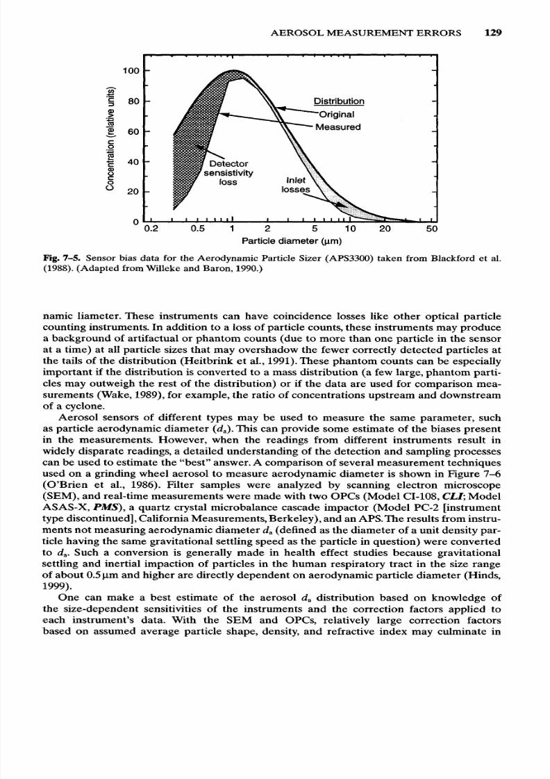
namic Particle Sizer (APS, TSI), a time-of-flight aerosol spectrometer that uses light scat-tering to detect particles. To illustrate the effect of a sensor's size-dependent sensitivity, alognormal size distribution with mass median aerodynamic diameter d50 = 1 urn and cjg = 2.5is calculated to simulate the m easured aeroso l (Fig. 7-5 ). Based on measured efficiency curvesof Blackford et al. (1988), there is a modification of the "measured" size distribution at thelow end due to a lack of detector response and at the high end due to a loss of particles atthe instrument inlet. No te that n either of these losses changes rapidly with particle size andthat the resulting d istribution appears nearly lognorm al. These modifications of the shape ofthe distribution may result in incorrect interpretation of the shape of the original aerosoldistribution.

If the sensor is an optical device receiving a light-scattering signal each time a particlepasses through the view volume, particle coincidence (i.e., simultaneous p resence of two ormore particles in the view volume) may result in the detection of a single larger particle,producing a slight shift to larger sizes and reducing the observed particle number over theentire size range. The importance of coincidence effects increases with particle n umb er con-centration.

In a time-of-flight device, such as the APS or the Aerosize r (TSf), the time of flight of aparticle accelerated between two path-intersecting laser beams is a measure of its aerody-

Original

aerosold50 = 5 um

On Mannequin

Free hangingClosed faceOpen face

Sampled by37 mm cassette

Q = 2L/min

Concentration (relative

units)

LIVE GRAPHClick here to view

http://knovel2/view_hotlink.jsp?hotlink_id=429369383





Particle diameter (jxm)

Fig. 7-5. Sensor bias data for the Aerodynamic Particle Sizer (APS3300) taken from Blackford et al.(1988). (Adapted from Willeke and Baron, 1990.)

namic liameter. These instruments can have coincidence losses like other optical particle

counting instruments. In addition to a loss of particle counts, these instruments may producea background of artifactual or phantom counts (due to more than one particle in the sensorat a time) at all particle sizes that may overshadow the fewer correctly detected particles atthe tails of the distribution (Heitbrink et al., 1991). These phantom counts can b e especiallyimpo rtant if the distribution is converted to a mass distribution (a few large, phan tom parti-cles may outweigh the rest of the distribution) or if the data are used for comparison mea-surements (Wake, 1989), for example, the ra tio of concen trations upstream and downstreamof a cyclone.

Aerosol sensors of different types may be used to measure the same parameter, suchas particle aerodynamic diameter (d a). This can provide some estimate of the biases present

in the measurements. However, when the readings from different instruments result inwidely disparate readings, a detailed understanding of the detection and sampling processescan be used to estimate the "best" answer. A comparison of several measu rement techniquesused on a grinding wheel aerosol to measure aerodynamic diameter is shown in Figure 7-6(O'Brien et al., 1986). Filter samples were analyzed by scanning electron microscope(SEM), and real-time measurements were made with two OPCs (Model CI-108, CLI; ModelASAS-X, PMS), a quartz crystal microbalance cascade impactor (Model PC-2 [instrumenttype discontinued], California Measurements, Berke ley), and an APS.The results from instru-ments not measuring aerodynamic diameter da (defined as the d iameter of a unit density par-ticle having the same gravitational settling speed as the particle in question) were convertedto da. Such a conversion is generally made in health effect studies because gravitationalsettling and inertial impaction of particles in the human respiratory tract in the size rangeof about 0.5 um and higher are d irectly depend ent on aerodynam ic particle diam eter (Hinds,1999).

One can make a best estimate of the aerosol da distribution based on knowledge ofthe size-dependent sensitivities of the instruments and the correction factors applied toeach instrument's data. With the SEM and OPCs, relatively large correction factorsbased on assumed average particle shape, density, and refractive index may culminate in

Distribution

Original

Measured

Inletlosses

Detectorsensistivity

lossConcentration (relative

units)



Aerodynamic diameter, da (um)

Fig. 7-6 . Measurement of grinding wheel dust using six different measuremen t techniques, including ascanning electron m icrograph (SEM ), two optical particle counters (OP C), a quartz crystal microbalancecascade impactor (QCM), and an APS3300 (APS). (Adapted from O'Brien et al., 1986.)

relatively unsatisfactory results. The grinding aerosol was a difficult aerosol for such acomparison because of the presence of a number of materials with widely disparateproperties.

Particle Statistics

Assuming that particles in an aerosol have been detected by a direct reading instrumen t, the

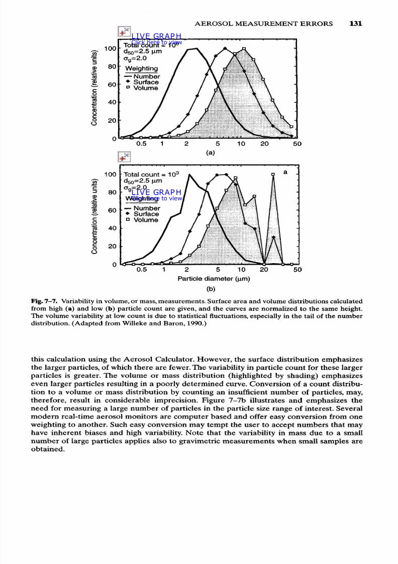
distribution of particles can be simulated using the Aeroso l Calculator spreadsheet indicatedabove. For a lognormal aerosol size distribution with a num ber median diameter of 2.5 umand a geometric standard deviation of 2.0, the sm ooth number distribution curve calculatedin Figure 7-7a results from a relatively large total count of 1 million particles distributed in19 size increm ents over th e size range 0.2 to 45 um. Such a high particle count is realistic fordynamic sensors whose data acquisition systems permit multichannel analysis, but mightoverload a filter that must be analyzed by microscopy.

The surface area and th e volume for each particle size may now be calculated. The surfacearea and volume of each size, multiplied by the number of particles in the respective sizeranges, results in the distributions also shown in Figure 7-7a. The p eak of each distributionis normalized to 100 relative units for illustration purposes. Inclusion of the particle densitywould allow conversion of the volume to a mass distribution. The representation of theaerosol size distribution by any of these weightings (count, surface, or volume) results in asmooth curve because a large number of particles was used.

When the total count is reduced to 1000 (Fig. 7-7b), the number distribution curve isstill recognizable as approximately lognormal, although the additional variability due toa smaller count in each size increment is apparent. Example 7-1 indicates how to perform

SEM

OPC

LASER OPCQCM

APS

Num

ber concentration (No./cm

3)







Particle diameter (urn)

(b)

Fig. 7-7 . Variability in volume, or mass, measurem ents. Surface area and volume d istributions calculatedfrom high (a) and low (b) particle count are given, and the curves are normalized to the same height.

The volume variability at low count is due to statistical fluctuations, especially in the tail of the numberdistribution. (Adapted from Willeke and Baron, 1990.)

this calculation using the Aerosol Calculator. However, the surface distribution emphasizesthe larger particles, of which the re are fewer. The variability in particle count for these largerparticles is greater. The volume or mass distribution (highlighted by shading) emphasizeseven larger particles resulting in a poorly determined curve. Conversion of a coun t distribu-tion to a volume or mass distribution by counting an insufficient number of particles, may,therefore, result in considerable imprecision. Figure 7-7b illustrates and emphasizes theneed for measuring a large num ber of particles in the particle size range of interest. Severalmodern real-time aerosol monitors are computer based and offer easy conversion from oneweighting to another. Such easy conversion may tempt the user to accept numbers that mayhave inherent biases and high variability. Note that the variability in mass due to a smallnumber of large particles applies also to gravimetric measurements when small samples areobtained.

Total count= 106

d50=2.5 urnoq=2.0

Weighting

NumberSurfaceVolume

Total count= 103

d50=2.5 jimag=2.0

Weighting

NumberSurfaceVolume

Concentration (relative units)



LIVE GRAPH

Click here to view









where n is usually chosen to be a number 3 and RAND 1 is a random number between 0and 1 that can be generated by the computer. The larger the value of n, the closer theresulting distribution will approximate a normal distribution, especially in the tails of thedistribution. The Poisson distribution approaches a norm al distribution for large particlecounts, so this function provides a reasonable approximation to a Poisson distribution.Poisson statistics require that the variance of the particle counts be equal to the meancount. Thus the stand ard deviation of the count in each bin is equal to the square root of

the value of the density function, i.e., the count in that bin. The function is rounded tointeger values as would be produced by a counting instrument.

EXAMPLE 7-1

Calculate the num ber, surface and volume values for a lognormal distribution of spheri-cal particles with a count m edian d iameter of 5 um and ag of 2. Simulate the variability as

if the entire distribution contains approximately 1000 particles.

Answer: The following equations were developed in the spreadsheet program Excel(Microsoft Corp., Bellevue, WA) and were implemented in the Aerosol Calculatorsizedis.xl modu le (see C hap ter 2 ). The inp ut values and constants are listed in the firstfour rows in the listing below. First we need to generate the diameters for w hich the log-normal distribution is produced. Column A has numbers starting at 0.25 with each fol-lowing row multiplied by a constant factor, in this case 1.32, giving 19 size intervals or binsbetween 0.25 and 49 urn. The starting size and size interval can b e changed to span therange of other size distributions if desired. The second column is the geom etric mean of

the upper and lower endpoints of each bin and is the size used to rep resent that b in. Thus,A6 to A7 is the first size interval and the geometric center of that interval is B6= ^JAIx A 6. C6 uses Eq. 7-1 to determ ine the concentration function in that bin or sizeinterval.

The " $" indicates that the reference does no t change in the following rows, i.e., in C7, C8,etc. The concentration function is normalized to give the appropriate number of totalcounts, in this case 1000.

C25 is the sum of all the values in column C. Next "noise" is added to the normalized par-ticle density function to simulate th e counting process. The following function prod ucesa random number that is part of an approximately normal distribution, centered aboutzero with a standard deviation o (Hansen, 1985)

where R AN D() is a function that generates a random number between 0 and 1. E6 is thevalue for the number distribution. The surface and volume distributions are calculatedfrom this distribution assuming spherical particles.



Finally, if onewishes tonormalize thepeak value of thedistributions to the same value,e.g., 100, as inFigure 7-7, three more columns, H, I, J can be created that contain the nor-

malized number, surface and volume distributions. These have not been included in the

table below due to space considerations. H6,16, and J6 would contain E6-100 / $E$25,F6 • 100 / $F$25,and G6• 100 / $G$25, respectively. E 25, F25 and G25contain themaximumvalues in their respective columns. No te tha t the columns E, F and G (as well as H, I and

J) will always appear somew hat different than indicated below since the random numberswill produce different results.

Further, sampling or detection efficiencies such as those indicated in Figure 7 ^ and

7-5 can becalculated bymultiplying thenormalized density function (column C) by thoseefficiencies.

T A B L E 7-1. Spreadsheet Size Distribution Calculation from Example 7-1 (Using the Aerosol

Calculator D escribed in Chapter 2)

1

2

3

45

6

7

8

9

10

11

1213

14

15

16

17

18

19

20

21

22

2324

25

A

d(50) =

o(g) =

total

0.2500

0.3300

0.4356

0.5750

0.7590

1.0019

1.3225

1.7457

2.3043

3.0416

4.0149

5.2997

6.9956

9.2342

12.189

16.090

21.238

28.035

37.006

48.850

B

5

2

n u m b e r of

d iame te r

(urn)

0.2872

0.3791

0.5005

0.6606

0.8720

1.1511

1.51942.0056

2.6474

3.4946

4.6128

6.0889

8.0374

10.609

14.004

18.486

24.401

32.20942.517

C

SQRT (2*TT) =

LN (d(50)) =

LN (a (g ) ) =

part icles =

Af

3E-05

0.0002

0.0006

0.0023

0.0067

0.0170

0.03660.0673

0.1052

0.1403

0.1592

0.1540

0.1268

0.0890

0.0532

0.0271

0.0117

0.0043

0.0014

1.0027

D

N u m b e r

0.03

0.16

0.65

2.25

6.69

16.93

36.5067.08

104.96

139.88

158.79

153.54

126.45

88.71

53.01

26.98

11.70

4.32

1.36

1,000

E

2.5066

1.6094

0.6931

1000N o. With

R a n d o m

C o u n t

0

1

1

3

4

19

3071

110

119

154

156

122

81

62

19

14

5

0

156

F

Surface

0

0.452

0.787

4.113

9.556

79.09

217.6897.2

2,422

4,565

10,294

18,170

24,759

28,643

38,200

20,397

26,188

16,2960

38,200

G

Volume

0

0.029

0.066

0.453

1.389

15.17

55.10299.9

1,069

2,659

7,914

18,439

33,167

50,646

89,161

62,843

106,502

87,482

0

106,502



Corrections for Density and Other Physical Properties

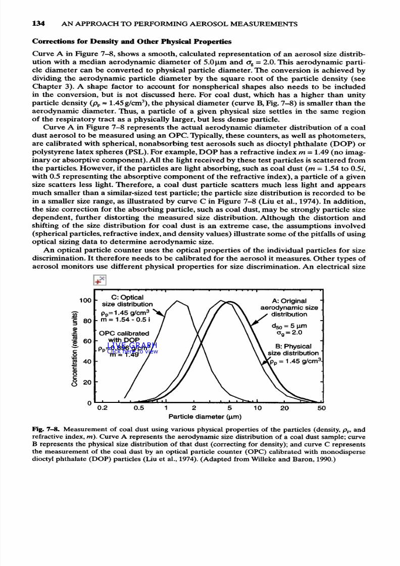
Curve A in Figure 7-8, shows a smooth, calculated represen tation of an aerosol size distrib-ution with a m edian aerodynamic diameter of 5.0 um and ag = 2.0. This aerodynamic parti-cle diameter can be converted to physical particle diameter. The conversion is achieved by

dividing the aerodynamic particle diameter by the square root of the particle density (seeChap ter 3). A shape factor to account for nonspherical shapes also needs to b e includedin the conversion, but is not discussed here. For coal dust, which has a higher than unityparticle density ( p p« 1.45 g/cm 3), the physical diam eter (curve B, Fig. 7-8) is smaller than theaerodynamic diameter. Thus, a particle of a given physical size settles in the same regionof the respiratory tract as a physically larger, but less dense particle.

Curve A in Figure 7-8 represents the actual aerodynamic diameter distribution of a coaldust aerosol to be m easured using an OP C. Typically, these counters, as well as photometers,are calibrated with spherical, nonabsorbing test aerosols such as dioctyl phthalate (DOP) orpolystyrene latex spheres (PS L). For exam ple, D O P has a refractive index m = 1.49 (no imag-

inary or absorptive com ponent). All the light received by these test particles is scattered fromthe particles. However, if the particles a re light absorbing, such as coal dust (m = 1.54 to 0.5/,with 0.5 representing the absorptive com ponent of the refractive index), a particle of a givensize scatters less light. Therefore, a coal dust particle scatters much less light and appearsmuch smaller than a similar-sized test particle; the particle size distribution is recorded to bein a smaller size range, as illustrated by curve C in Figure 7-8 (Liu et al., 1974). In addition,the size correction for the absorbing particle, such as coal dust, may be strongly particle sizedepen dent, further distorting the m easured size distribution. Although the d istortion andshifting of the size distribution for coal dust is an extreme case, the assumptions involved(spherical particles, refractive index, and density values) illustrate some of the pitfalls of usingoptical sizing data to determine aerodynamic size.

An optical particle counter uses the optical properties of the individual particles for sizediscrimination. It therefore needs to b e calibrated for the aerosol it measures. Other types ofaerosol monitors use different physical properties for size discrimination. An electrical size

Particle diameter (urn)

Fig. 7-8. Measurement of coal dust using various physical properties of the particles (density, p p, andrefractive index, m). Curve A rep resents the aerodynamic size distribution of a coal dust sample; curveB represents the physical size distribution of tha t dust (correcting for density); and curve C representsthe measurement of the coal dust by an optical particle counter (OPC) calibrated with monodispersedioctyl phthalate (DO P) particles (Liu et al., 1974). (Adapted from Willeke and Baron , 1990.)

A: Originalaerodynamic size

distribution

B: Physicalsize distributionjpp = 1.45 g/cm

3-

C: Opticalsize distribution

OPC calibratedwith DOP

pp=0.896 g/cm3'

m = 1.49








classifier, for example, uses the electrical mobility of particles for size discrimination ofsubmicrometer aerosols. Because the composition of the aerosol to be measured may beunknown, inadequate calibration may prevent the "size" obtained with one type of aerosolmonitor from equaling the "size" obtained with another instrument.

Presentation of Size Distribution Data

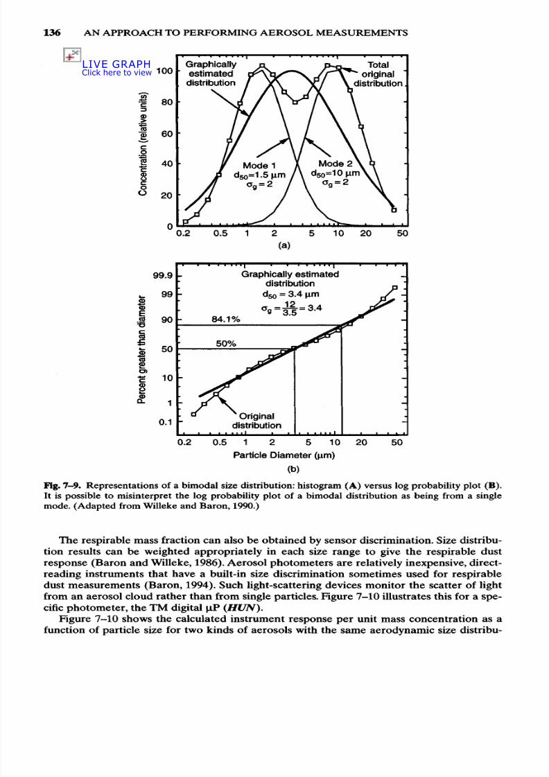
There are several ways of presenting measured size distributions, each with advantages anddisadvantages (see C hapter 22). Assum e that two dusts are present in the air: dust 1 with amedian diameter of 1.5 urn and dust 2 with a median diameter of 10 um, both with a geo-metric standard deviation of 2.0. Measurement of the aerosol with a direct-reading aerosolsize spectrometer is simulated using the Aerosol Calculator to give the bimodal size distrib-ution shown in Figure 7-9A.

If this measurement is replotted on a cumulative plot where the value of the ordinate

indicates the number of particles less than the given size, the wavy plot of Figure 7-9Bresults. Starting with the smaller particles, the curve increases with increasing particle sizein an S-shaped manner. At sizes slightly larger than the median size of dust 1 the curve levelsoff and then increases in slope again as the m edian size of dust 2 is approached. This type ofpresentation is common for the results of low-resolution instruments such as a cascadeimpactor.

If one does not know tha t there are two dust modes present, one may be tempted to drawa straight line through the cum ulative plot, as indicated by the heavy straight line in Figure7-9B. This is frequently done and justified by attributing the deviation of the data from astraight line to experimental variability. The resulting graphically estimated or "measured"

aerosol thus has a geom etric m edian diameter of about 3.4 (im (corresponding to theminimum between the two dusts) and a geometric standard deviation of 3.5, indicating asingle dust distribution much bro ader than each of the m odes in the o riginal bimodal distri-bution. Potentially valuable information is lost in this representation of the da ta because m ul-tiple modes usually indicate different sources of aerosol.

Some statistical tests may also indicate that the cumulative data in Figure 7-9B do notfit a single distribution. For instance, the Kolmogorov-Smirnov test (Gibson, 1971) wouldindicate whether the measured distribution fits a single mode distribution, and a plot ofresiduals (the differences between the measured and calculated values) qualitativelyindicates whether adjacent m easurem ents in the curve are correlated or whether the data fit

the single lognormal distribution model.Both types of represen tation have advan tages and disadvantages. The differential plot

gives a better presentation of the distribution shape: Modes show up directly, and any effectof bias is constrained to a narrow size range and is not prop agated throughout the en tire sizedistribution as in the cumulative plot. The cumulative plot provides a better estimate of themedian diameter of the aerosol and allows easier presentation of data graphically withoutusing a computer. Frequently, investigation of the data through several display techniquesaffords a more complete understanding of the physical meaning of the data.

Particle Size Selection

The type of aerosol m onitor used depends on the purpose of sampling. The industrial hygien-ist generally samples from a health perspective. Because the physiological shape of the humanrespiratory system determines the region in which the particles will deposit, a pre-classifieris frequently mounted ahead of the sensor in order to intentionally limit the particle mea-surement to particles reaching the physiological region of concern. For example, a cyclone,impactor, or elutriator pre-classifier can separate the aerosol into respirable and nonres-pirable fractions.



Particle Diameter (urn)

(b)

Fig. 7-9 . Represen tations of a bimodal size distribution: histogram (A ) versus log probability plot (B) .

It is possible to misinterpret the log probability plot of a bimodal distribution as being from a single

mode. (Adapted from Willeke and Baron, 1990.)

The respirable mass fraction can also be obtained by sensor discrimination. Size distribu-tion results can be weighted appropriately in each size range to give the respirable dustresponse (Baron and W illeke, 1986). Aerosol p hotom eters are relatively inexpensive, direct-reading instruments that have a built-in size discrimination sometimes used for respirabledust m easurem ents (Baron , 1994). Such light-scattering devices mon itor the scatter of lightfrom an aeroso l cloud rath er than from single particles. Figure 7-10 illustrates this for a spe-cific photom eter, the TM digital u P (HUN).

Figure 7-10 shows the calculated instrument response per unit mass concentration as afunction of particle size for two kinds of aerosols with the same aerodynamic size distribu-

Originaldistribution

Graphically estimateddistribution

Percent greater than diam

eter

Totaloriginal

distribution

Mode 2Model

Graphicallyestimateddistribution

Concentration (relative u

nits)







Mass median diameter (jim)

Fig. 7-11. Bias map comparing two defined respirable dust response curves for a range of lognormalsize distributions. Data points represent distributions reported by (•) Hinds and Bellin (1988) and (+)Bowman et al. (1984).

tion (d 50 = 5 Jim, <jg = 2.0): non-light-absorbing D O P droplets and dense, light-absorbing ironoxide (Fe2O3) particles (Arm bruster, 1987). The decline in response with increasing particlesize above about l^im is common to all photometers. This decrease approximately corre-sponds to the classification characteristics of the ACGIH and BMRC definitions for res-pirable dust (A CG IH, 1999a,b), also indicated on Figure 7-9. Complex interactions betweenthe incident light and the particle result in similarly complex response curve patterns thatdiffer from one type of aerosol to another.

A photometer calibrated with one type of aerosol will, therefore, generally be biased ifused to measure another aerosol with different chemistry or size distribution. This bias canbe adjusted for a specific aerosol by drawing the aerosol through a filter downstream of or

Fig. 7-10. Respirable mass response using a photom eter for example size distributions of two m aterials

with dp = 5um, crg = 2.0. Detection efficiency is for the TM Digital uP from the H und Corp. Based onmeasurem ents by Arm bruster (1987). Two definitions of respirable dust are also included. (Adap ted fromWilleke and Baron, 1990.)

Geom

etric standard dev

iation

2

Relative Response per mg/m

Relative Efficiency (%)

Photometer Response

DOPF e 2 O 3

Sampling Efficiency

CriteriaACGIH

BMRC



parallel to the sensor and adjusting the sensor readout to equal the concentration measuredusing the filter. This procedure is valid as long as the type and size distribution of the aeroso lremain unchanged. Instruments of this type can be used to make relative measurem ents, oftenproviding useful real-time information, but should be used only with great care for situationsrequiring high accuracy.

One approach to evaluating the accuracy of a method over a wide range of aerosol sizedistributions is the use of a bias m ap (Caplan et al., 1977).This involves determining the rangeof size distributions over which the measurement is expected to occur. Hinds and Bellin(1988) reviewed aerosol distributions in more than 30 workplace operations and found sizedistributions with crg ranging from 1.5 to 5 and mass median aerodynam ic diam eters rangingfrom 0.1 to 20. One can examine the bias resulting from measurement of lognormal distrib-utions throughou t this range by comparison of one sampler versus a standard. As an example,calculation of the bias of the ACGIH definition versus the BMRC definition (Fig. 7-10) foreach size distribution can be used to produ ce the bias map in Figure 7-11 . This approach has

been used to evaluate the optimum flow rate through a cyclone by comparing bias maps ofthe cyclone relative to a respirable dust definition at different flow rates (B artley e t al., 1994).Hinds and Bellin (1988) used their size-distribution data to estimate the effectiveness of res-pirators with measured size-dependent leakage.

REFERENCES

ACGIH. 1999a. Particle Size-Selective Sampling of Paniculate Air Contaminants, ed. J. H. Vincent.

Cincinnati, OH : Am erican C onference of Governm ental Indu strial Hygienists.

ACGIH. 1999b. Threshold Limit Values for Chemical Su bstances and Physical Agents. Cincinnati, OH:

American Conference of Governmental Industrial Hygienists.

Arm bruster, L. 1987. A new generation of light-scattering instruments for respirable dust m easurement.

Ann. Occup. Hyg. 31:181-193.

Baron, P. A. 1984. Aerosol Photom eters for respirable dust measurem ents. In Manu al of Analytical

Methods, 3rd Ed. (DHHS/NIOSH Pub. No. 84-100). Cincinnati, OH: National Institute for

Occupational Safety and Health.

Baron, P. A. 1994. Asbestos and other fibers by PCM , Method 7400, Issue 2: 9/15/94. NIOSH Manual of

Analytical Methods, 3d eD ., ed. P. M. Eller. (NIOSH ) Pub. 84-100. Cincinnati, OH : National Institutefor Occupational Safety and Health.

Baron, P. A. and G. J. Deye. 1990. Elec trostatic effects in asbestos sampling I: Experimental

measurements. Am. Ind. Hyg. Assoc. J. 51:51-62.

Baron , P. A. and K. Willeke. 1986. Respirable droplets from whirlpools: Measurements of size

distribution and estimation of disease potential. Environ. Res. 39:8-18.

Bartley, D. L., C - C Chen, R. Song, and T. J. Fischback. 1994. Respirable aerosol sam pler performance

testing. Am. Ind. Hyg. Assoc. J. 55(ll):1036-1046.

Blackford, D., A. E. Han sen, D . Y. H. Pui, P.Kinney, and G. P. An anth. 1988. Details of recent work towards

improving the performance of the TSI Aerodyn amic Particle Sizer. In Proceedings of the2nd AnnualMeeting of the Aerosol Society.Bournemouth, U.K., March 22-24.

Bowman, J. D., D. L. Bartley, G. M. Breuer, L. J. Doemeny, D. J. Murdock. 1984. Accuracy criteriarecommended for the certification of gravimetric coal mine dust samplers. Internal Report availablefrom National Technical Information Service NTIS PB 85-222446. Cincinnati: National Institute for

Occupational Safety and Health.

Buchan, R. M., S. C Soderholm, and M. J. Tillery. 1986. Aerosol sampling efficiency of 37m m filter

cassettes. Am. Ind. Hyg. Assoc. J. 47:825-831.

Caplan , K. J., L. J. Doemeny, and S. D. Sorensen . 1977. Performance characteristics of the 10 mm cyclonerespirable sampler: Part I—M onodisperse studies. Am. Ind. Hyg. Assoc. J. 38(2):83-95.



Currie, L. A. 1992. In pursuit of accuracy: Nom enclature, assumptions and standards. Pure Appl. Chem.

64:455-472.

Eisenhart, C, H. H. Ku, and R. Colle. 1990. Expression of the uncertainties of final measurementresults: Reprints. In SelectedPublications for the EMAP Workshop. NIST Internal Report 90-4272.

Washington, DC: National Institute for Standards and Technology.

EPA. 1994. Guidance for the Data Quality Objectives Process, EPA QA/G4, in EPA/600/R-96/055.

(Available at http://www.epa.gov/regionlO/www/offices/oea/qaindex.htm)

Gibson, J. D. 1971. NonparametricStatistical Inference.New York: McGraw-Hill.

Hansen , A. G. 1985. Simulating the normal distribution. BYTE October:137-138.

He itbrink, W. A., P. A. Baron, and K. Willeke. 1991. Coincidence in time-of-flight aerosol spectrometers:

phantom particle creation. Aerosol ScLTechnol 14:112-126.

Hinds, W. C. 1999. Aerosol Technology. New York: John Wiley & Sons.

Hinds, W. C. and P. Bellin. 1988. Effect of facial-seal leaks on p rotec tion provided by half-mask

respirators. Appl. Ind. Hyg. 3:158-164.

Liu, B. Y. H., V. A. Marple, K. T. Whitby, and N. J. Barsic. 1974. Size distribution measurement of airborne

coal dust by optical particle counters. Am. Ind. Hyg. Assoc. J. 8:443-451.

Liu, B. Y. H., D. Y. H. Pui, and W. Szymanski. 1985. Effects of elec tric charge on sampling and filtration

of aerosols. Ann. Occup. Hyg. 29:251-269.

O'Brien, D. M., P. A. Baron, and K. Willeke. 1986. Size and concentration measurement of an industrial

aerosol. Am. Ind. Hyg. Assoc. J. 47:386-392.

Okazaki, K., R. W. Wiener, and K. Willeke. 1987a. Isoaxial aerosol sampling: Non-dimensional

representa tion of overall sampling efficiency. Environ. ScL Technol. 21:178-182.

Okazaki, K., R. W. Wiener, and K. Willeke. 1987b. Non-isoaxial aerosol sampling: Mechanisms

controlling the overall sampling efficiency. Environ. ScL Technol. 21:183-187.

Pui, D. Y. H. 1996. Direct-reading instrumentation for workplace aerosol measurements—A review.

Analyst 121:1215-1224.

Vincent, J. H. 1989. Aerosol Sampling: Science and Practice. New York: John W iley & Sons.

Wake, D. 1989. Anom alous effects in filter penetration measurem ents using the aerodynamic particle

sizer (APS 3300). /. Aerosol ScL20:1-7.

Willeke, K. and P.A. Baron . 1990. Sampling and interpretation errors in aerosol sampling. Am. Ind. Hyg.

Assoc. I. 51:160-168.

Willeke, K. and B. Y H. Liu. 1976. Single particle op tical cou nter: Principles and application. In Fine

Particles: Aerosol Generation, Measurem ent, Sampling and A nalysis, ed. B. Y. H. Liu. New York:

Academic Press.

Williams, K., C. Fairchild, and J. Jaklveic. 1993. Dynamic mass measurement techniques. In Aerosol

Measurement, eds. K. Willeke and P. Baron. New York: Van No strand Reinhold.

ch07_an approach to performing aerosol measurements

Documents