cfd modelling of natural convection in air cavitiesusir.salford.ac.uk/35008/1/347-1300-1-pb.pdf ·...

CFD modelling of natural convection in air cavities

Ji, Y

Title CFD modelling of natural convection in air cavities

Authors Ji, Y

Type Article

URL This version is available at: http://usir.salford.ac.uk/35008/

Published Date 2014

USIR is a digital collection of the research output of the University of Salford. Where copyright permits, full text material held in the repository is made freely available online and can be read, downloaded and copied for noncommercial private study or research purposes. Please check the manuscript for any further copyright restrictions.

For more information, including our policy and submission procedure, pleasecontact the Repository Team at: [email protected].

mailto:[email protected]

Yingchun Ji CFD Letters Vol. 6(1) 2014

15

www.cfdl.issres.net Vol. 6 (1) – March 2014

CFD Modelling of Natural Convection in AirCavitiesYingchun Ji1c

1 School of the Built Environment, University of Salford, U.K

Received: 06/08/2013 – Revised 25/12/2013 – Accepted 03/02/2014

Abstract

This paper discusses the modelling of natural convection in air cavities using four eddyviscosity turbulence models. Two 2D closed cavities with deferentially heated wallsopposite each other and one 3D open ended tall cavity with one side is heated and adiabaticfor all the others were investigated. The CFD simulation results for the two 2D cases werecompared with their corresponding experimental measurements and it was found that the k-omega turbulence model offered the best solution among the turbulence models tested.Close agreement was also achieved between the k-omega model and the experiments in theprediction of temperature and velocity fields for the 3D case with Monte Carlo radiationmodel. The work has demonstrated the ability of the eddy viscosity turbulence models formodelling natural convection and radiation in different types of cavities.

Keywords: Cavity; Natural Convection; Radiation; Turbulence model; CFD.

1. Introduction

Natural convection in air cavities has been the subject of much research in recent decades dueto its various engineering applications, such as solar chimneys, double skin façades, and Trombewalls. Understanding the underlying flow characteristics of these types of engineering applicationsare important for engineers and architects to design low energy ventilation, cooling and heating forbuildings [1]. It is difficult to analytically solve natural convection in these types of engineeringflows due to their complex physical mechanisms therefore experimental investigations were oftenused. A closed rectangular cavity with an aspect ratio 5 between its height and width were studiedby [2] in which temperature and velocity profiles were measured at the mid height of the cavity.Similar investigations for temperature distribution and local heat transfer rate in a rectangular cavitywere also performed by [3] and [4]. Among these works the natural convection heat transfer wasstudied by varying the surface temperature differences between cavity walls. The inner surfaces ofthese testing rigs were made by aluminium alloy plate which tends to have a small emissivity(normally less than 0.1) therefore the heat transfer within the cavity was dominated by naturalconvection, and with the given temperature difference radiation effects from the internal walls werenot examined. However, the surface radiation flux between cavity walls may have an impact on thetemperature and velocity distribution when the inner surfaces of the cavity have a relatively largeemissivity. The experiments of [5] were conducted on a square cavity with differentially heatedvertical walls. The inner surfaces of the cavity were made by steel plates. In average the emissivity

c Corresponding Author: Y.JiEmail: [email protected] Telephone: +44 116 295 4841 Fax: +44 116 295 4841© 2014 All rights reserved. ISSR Journals PII: S2180-1363(14)6015-X

CFD Modelling of Natural Convection in Air Cavities

16

of steel plate ranges from 0.7 to 0.8. With a 40 degree temperature difference between the hot walland the cold wall, radiation effect may not be ignored for this case. The work of [6] investigatednatural convection heat transfer and surface radiation in a three dimensional tall cavity with anaspect ratio of 16 between the height and width of the cavity. In the experiments both temperaturesand emissivities of cavity wall surfaces were varied in order to quantify the convective and radiativeheat fluxes of cavity wall surfaces. It is worth to note that there were cases in [6] the radiative heatfluxes were larger than the convective heat flux.

Cavity air flow and heat transfer were also investigated extensively using computational fluiddynamics (CFD). With the recent advances in computing power, the process of creating a CFDmodel and analysing the results is much less labour-intensive, reducing the time and therefore thecost. Some parameter investigations like change of geometrical factors, change of boundaryconditions, which may be difficult to perform by using experimental studies, could be introducedusing CFD modelling. Examples of CFD studies include the work of [7-10]. Among these studies,researchers were focusing on solving the natural convection heat transfer and/or radiation indifferent kind of cavities using different turbulence models, showing the capability of a specificmodel for specific cases. The current investigations are to evaluate the relative accuracy for thewidely used turbulence models in engineering practices when modelling natural convection heattransfer with or without radiation in three typical cavities. Comprehensive details for using theturbulence models are presented and the modelling results are compared with the availableexperimental measurements, through which we may identify which model will be the better suitedmodel for these types of airflows.

2. Experiments

Figures 1 shows the closed 2D cavity from [2] where only natural convection was considered(Fig 1a), the closed 2D cavity from [5] and the open-ended 3D cavity from [6] where both naturalconvection and radiation were considered (Figs 1b & 1c).

Figure 1. (a) 2D rectangular cavity, (b) 2D square cavity and (c) 3D tall cavity

In the study of [2] the aspect ratio of height and width was 5.0 with a 45.8 ºC temperaturedifference between the hot and the cold aluminium alloy walls. The top and bottom of the cavitywere well insulated and the heat losses and gains were ignored. The depth of the cavity wassufficiently long so that in the central region of the depth the airflow could be assumed to be twodimensional. A square cavity (aspect ratio is 1.0) was used in [5] and the temperature difference is


17

40ºC between the two vertical steel plate walls. Other setups were similar with [2] in order toachieve a 2D flow at the centre of the testing rig.

The open-ended cavity of [6] has an aspect ratio of 16. The cavity comprised a heated wall aty =0.5m and well insulated walls at y =0, x =0 and x =0.5 (Fig 1c). The top and bottom of thecavity are free openings which allow air to flow freely in any direction. In the experimental work,the emissivities of the cavity walls can be adjusted in order to examine the effects of radiation onthe buoyancy-induced natural convection flow, and the heated wall temperature can be fixed at anyvalue in the range of 100C - 175C. In this work the experimental measurements for the hot wallwith emissivity of 0.9 and temperature of 150C were used to compare with the CFD predictions.

3. CFD Modelling

The commercial CFD code Ansys CFX [11] was used to model the natural convectionairflows for the cases described in section 2.Two equation eddy-viscosity turbulence models areinvestigated in this work. They are k-epsilon based models: the standard k-epsilon model [12] andthe RNG k-epsilon model [13] and the k-omega based models: the k-omega model [14] and theShear Stress Transport (SST) model [15]. These turbulence models offer a good compromisebetween computational cost and accuracy, and are applicable to investigate engineering cavityflows such as Trombe walls, solar collectors/chimneys, and double skin façades. The applications ofthese technologies in buildings are gaining popularity in recent years with the focus of reducingbuilding carbon emissions [16, 17].

For steady-state natural convection applications, the two-equation models are formulated fromthe incompressible form of Reynolds Averaged Navier-Stokes (RANS) equation using the turbulenteddy-viscosity concept. The formulations of the eddy viscosity turbulence models have been wellreported therefore not introduced here. For details please refer either [11] or [18] where the detailedderivations of these models are available

3.1. Modelling of the 2D cavities

For the rectangular case, wall boundary with fixed temperatures (66.8C and 21C,Figure 1a) is used for left and right walls and symmetry plane boundary is used at front andback in order to perform 2D calculation. The top and bottom of the cavity are modelled asadiabatic walls.

Simulations use time steps to reach their steady-state in CFX. These time steps donot define a transient flow so do not have to be uniform. In fact, the time steps should be aslarge as possible without causing the solution process to become unstable. For buoyancy-driven airflows, the time step size can be estimated using a relationship

2/1max ))/(( TgLt [11], where L is a length scale, is the thermal expansion

coefficient and T is a temperature variation of the fluid. maxt is about 1.3s for the case of[2]. Higher values (5.0s) were used to speed up the calculation and a value of 1.0s was usedfor finding the final converged solution.

Similar modelling routines were employed for the square cavity case. In this case theoptimised time step is 1.25s. Due to the high emissivity of the internal finishes of this testingrig, radiation modelling was considered. A value of 0.75 was used for the emissivity of innersteel plate walls.

The convergence criteria for both cases are: i) all the maximum residuals are lowerthan 510-4 for the last 100 time steps and ii) the global domain imbalance for energyequation is less than 0.1%.


18

3.2. Modelling of the 3D cavity

The modelling methods used in the 2D cases are all applicable for the 3D case withthe following differences: Except the heated wall (Figure 1c) with fixed temperature allother vertical walls are simulated as ‘adiabatic’ due to the well insulated condition for them.The top and bottom of the cavity are ‘opening’ boundaries which allow air to flow freely inany direction according to the pressure difference across the openings. In practice whenfluids flow through sharp openings there will be losses in volume flow rate due to expansionor discharge of fluid flow at these openings. The losses can be represented by the losscoefficient f . A value of 2.4 was used for this study to estimate the pressure loss across theopening boundaries by a relation of 2/2

nl UfP (where nU is the normal component ofvelocity).

Due to the high emissivities (0.9) of vertical walls and the large temperaturedifferences between them, surface thermal radiation effects were taken into account for theCFD simulation. Thermal radiation model used in this research is the Monte Carlo (MC)Model. This model has wider engineering applications, particularly for radiation modellingin participating media and multi-domains with both transparent fluids and semi-transparentsolids, such as airflow in glasses with external solar radiation [19].

4. Mesh and its dependency test

Figure 2 shows the structured surface mesh for the 2D closed rectangular cavity of [2] and the3D open ended cavity of [6]. The mesh for the square cavity is similar as the rectangular cavity withthe same mesh density for the top and bottom walls. Due to the high aspect ratios of thesegeometries, only the upper parts of the geometries are shown here.

Figure 2 CFD surface meshes: (left) 2D rectangular cavity case and (right) 3D open ended case.

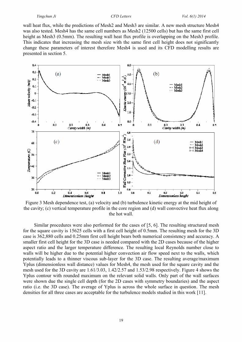
Mesh dependency investigations were conducted using k-omega turbulence model for the2D rectangular natural convection cavity. Mesh1 uses 3000 elements (25120) with the first cell towall distance 2.5mm. Mesh2 uses 12500K elements (50250) with the first cell to wall boundarydistance 1.0 mm. Mesh3 uses 28125 elements (75375) with 0.5mm first cell to wall distance. Theresulting velocity and turbulence kinetic energy profiles at the mid height of the cavity are shown infigures 3a, b. The velocity profiles for the three mesh sizes show negligible differences while theturbulence kinetic energy profiles show small differences (less than 5%). Vertical temperatureprofiles of the three meshes at the centre of the cavity were also examined. Mesh1 showsdifferences compared with Mesh2 and Mesh3 (figure 3c). Although the velocity, temperature andturbulence kinetic energy profiles are not sensitive to the mesh densities and the first cell height, thelocal wall convective heat flux shows significant dependency with both mesh density and the firstcell height at the lower region of the cavity (figure 3d). Clearly, Mesh1 results in a lower average


19

wall heat flux, while the predictions of Mesh2 and Mesh3 are similar. A new mesh structure Mesh4was also tested. Mesh4 has the same cell numbers as Mesh2 (12500 cells) but has the same first cellheight as Mesh3 (0.5mm). The resulting wall heat flux profile is overlapping on the Mesh3 profile.This indicates that increasing the mesh size with the same first cell height does not significantlychange these parameters of interest therefore Mesh4 is used and its CFD modelling results arepresented in section 5.

Figure 3 Mesh dependence test, (a) velocity and (b) turbulence kinetic energy at the mid height ofthe cavity; (c) vertical temperature profile in the core region and (d) wall convective heat flux along

the hot wall.

Similar procedures were also performed for the cases of [5, 6]. The resulting structured meshfor the square cavity is 15625 cells with a first cell height of 0.5mm. The resulting mesh for the 3Dcase is 362,880 cells and 0.25mm first cell height bears both numerical consistency and accuracy. Asmaller first cell height for the 3D case is needed compared with the 2D cases because of the higheraspect ratio and the larger temperature difference. The resulting local Reynolds number close towalls will be higher due to the potential higher convection air flow speed next to the walls, whichpotentially leads to a thinner viscous sub-layer for the 3D case. The resulting average/maximumYplus (dimensionless wall distance) values for Mesh4, the mesh used for the square cavity and themesh used for the 3D cavity are 1.61/3.03, 1.42/2.57 and 1.53/2.98 respectively. Figure 4 shows theYplus contour with rounded maximum on the relevant solid walls. Only part of the wall surfaceswere shown due the single cell depth (for the 2D cases with symmetry boundaries) and the aspectratio (i.e. the 3D case). The average of Yplus is across the whole surface in question. The meshdensities for all three cases are acceptable for the turbulence models studied in this work [11].


20

Figure 4 Yplus plots Cheesright case Mesh 4 (a), square cavity (b) and the 3D cavity (c).

5. Results and discussions

5.1 Two dimensional rectangular cavity

The temperature contour of the cavity shows that the air flow inside the cavity wasstrongly stratified due to the asymmetrical boundary conditions of hot and cold walls (figure5a) which gives a relatively linear temperature gradient in the core region along the verticalheight. The gradient is slightly increased at the upper and lower ends. This is consistent withthe temperature profiles shown in figure 3c. The velocity vector shown in figure 5b is on asample plane which does not reflect the real mesh information (the plots on the real meshwill be too dense to display properly). It simply shows the strength of air movement withinthe domain. At centre region of the mid height (also away from the wall boundaries) of thecavity the airflow shows the least motion due to the effects of the upstream and downstreamclose to the hot and cold walls (figure 5b). This is consistent with figure 3a.

Figure 5 Temperature field (a) and velocity vector (b) inside the cavity of the 2D case.

The turbulence diffusive potential is often measured by the turbulence viscositywithin the flow field, while the turbulence viscosity is determined through turbulencemodelling. Higher turbulence viscosities will increase the turbulence diffusivity andpotentially increase the thickness of the boundary layer. Figure 6 shows the scaled


21

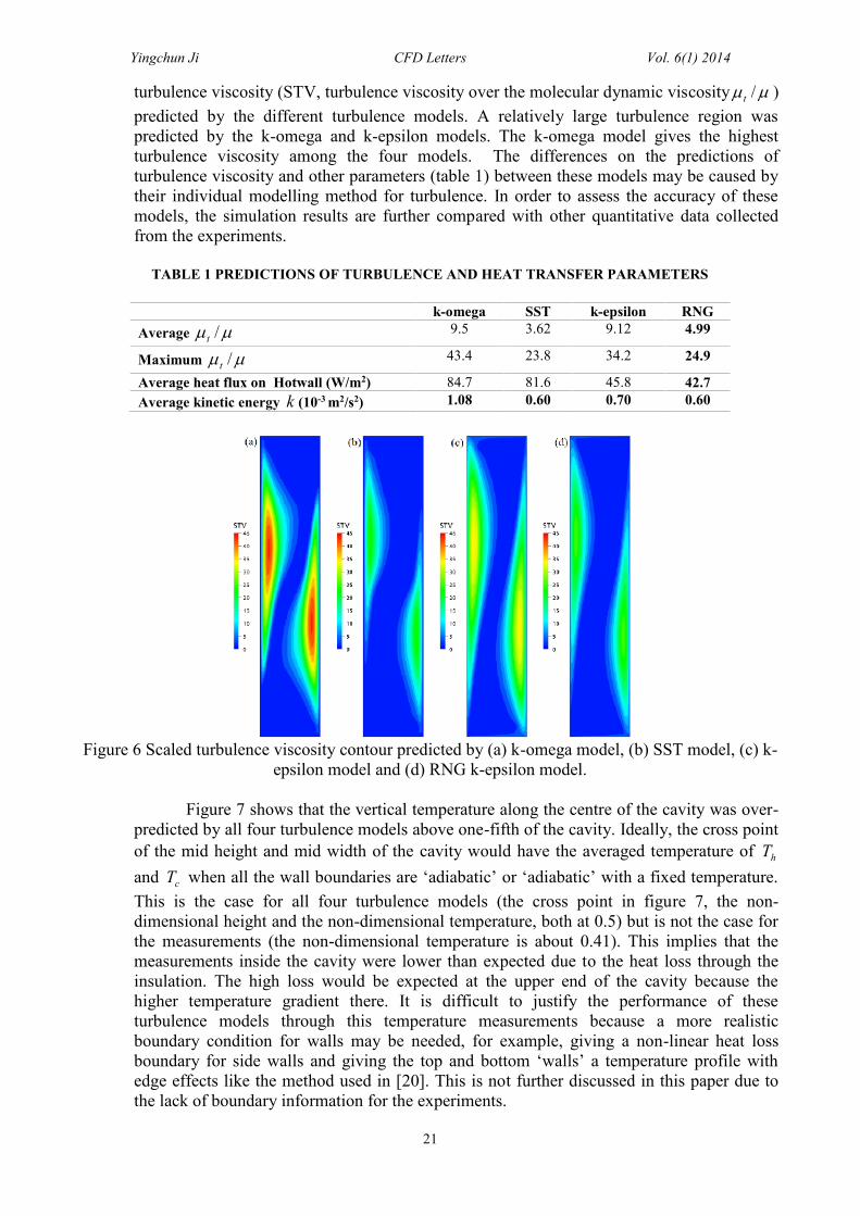
turbulence viscosity (STV, turbulence viscosity over the molecular dynamic viscosity /t )predicted by the different turbulence models. A relatively large turbulence region waspredicted by the k-omega and k-epsilon models. The k-omega model gives the highestturbulence viscosity among the four models. The differences on the predictions ofturbulence viscosity and other parameters (table 1) between these models may be caused bytheir individual modelling method for turbulence. In order to assess the accuracy of thesemodels, the simulation results are further compared with other quantitative data collectedfrom the experiments.

TABLE 1 PREDICTIONS OF TURBULENCE AND HEAT TRANSFER PARAMETERS

k-omega SST k-epsilon RNGAverage /t

9.5 3.62 9.12 4.99

Maximum /t43.4 23.8 34.2 24.9

Average heat flux on Hotwall (W/m2) 84.7 81.6 45.8 42.7Average kinetic energy k (10-3 m2/s2) 1.08 0.60 0.70 0.60

Figure 6 Scaled turbulence viscosity contour predicted by (a) k-omega model, (b) SST model, (c) k-epsilon model and (d) RNG k-epsilon model.

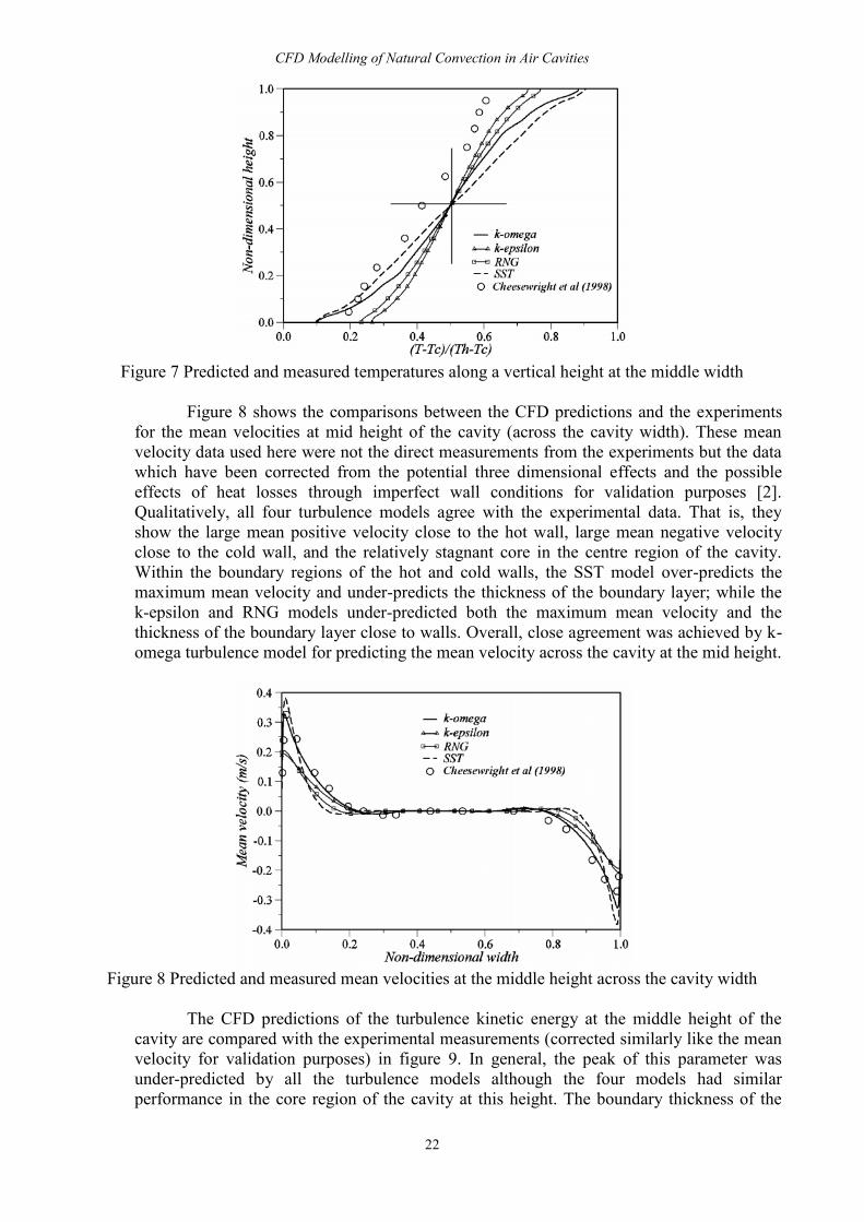
Figure 7 shows that the vertical temperature along the centre of the cavity was over-predicted by all four turbulence models above one-fifth of the cavity. Ideally, the cross pointof the mid height and mid width of the cavity would have the averaged temperature of hTand cT when all the wall boundaries are ‘adiabatic’ or ‘adiabatic’ with a fixed temperature.This is the case for all four turbulence models (the cross point in figure 7, the non-dimensional height and the non-dimensional temperature, both at 0.5) but is not the case forthe measurements (the non-dimensional temperature is about 0.41). This implies that themeasurements inside the cavity were lower than expected due to the heat loss through theinsulation. The high loss would be expected at the upper end of the cavity because thehigher temperature gradient there. It is difficult to justify the performance of theseturbulence models through this temperature measurements because a more realisticboundary condition for walls may be needed, for example, giving a non-linear heat lossboundary for side walls and giving the top and bottom ‘walls’ a temperature profile withedge effects like the method used in [20]. This is not further discussed in this paper due tothe lack of boundary information for the experiments.


22

Figure 7 Predicted and measured temperatures along a vertical height at the middle width

Figure 8 shows the comparisons between the CFD predictions and the experimentsfor the mean velocities at mid height of the cavity (across the cavity width). These meanvelocity data used here were not the direct measurements from the experiments but the datawhich have been corrected from the potential three dimensional effects and the possibleeffects of heat losses through imperfect wall conditions for validation purposes [2].Qualitatively, all four turbulence models agree with the experimental data. That is, theyshow the large mean positive velocity close to the hot wall, large mean negative velocityclose to the cold wall, and the relatively stagnant core in the centre region of the cavity.Within the boundary regions of the hot and cold walls, the SST model over-predicts themaximum mean velocity and under-predicts the thickness of the boundary layer; while thek-epsilon and RNG models under-predicted both the maximum mean velocity and thethickness of the boundary layer close to walls. Overall, close agreement was achieved by k-omega turbulence model for predicting the mean velocity across the cavity at the mid height.

Figure 8 Predicted and measured mean velocities at the middle height across the cavity width

The CFD predictions of the turbulence kinetic energy at the middle height of thecavity are compared with the experimental measurements (corrected similarly like the meanvelocity for validation purposes) in figure 9. In general, the peak of this parameter wasunder-predicted by all the turbulence models although the four models had similarperformance in the core region of the cavity at this height. The boundary thickness of the


23

kinetic energy close to wall was under-predicted by the SST turbulence model due to thefast dissipating of the turbulence eddies, which leads to lower turbulence intensity predictedby this model. The k-epsilon based model failed to resolve the wall boundary properly forthis case. The k-omega model gives a reasonable agreement except the maximum turbulencekinetic energy.

Figure 9 Predicted and measured kinetic energy at the middle height across the cavity width

Figure 10 shows the local convective heat flux predicted by different turbulencemodels along the heated wall surface. The predicted transient onsets (shown as the upperturning points for the local convective heat flux in figure 10) for the k-omega and SSTmodels are at 0.21 to 0.24 (dimensionless height), while the experiments gave a value of0.22 [21]. This implies that the k-omega based turbulence models gave reasonable closeprediction for the convective heat transfer and the transition onset. However, lowerconvective heat fluxes were predicted by the k-epsilon based turbulence models and thetransition onsets were not clearly identifiable.

Figure 10 Predictions of the local Nusselt number along the heated wall surface.

5.2 Two dimensional square cavity

The principle and modelling approach for this case were both similar as therectangular case apart from the involvement of radiation modelling. The predicted


24

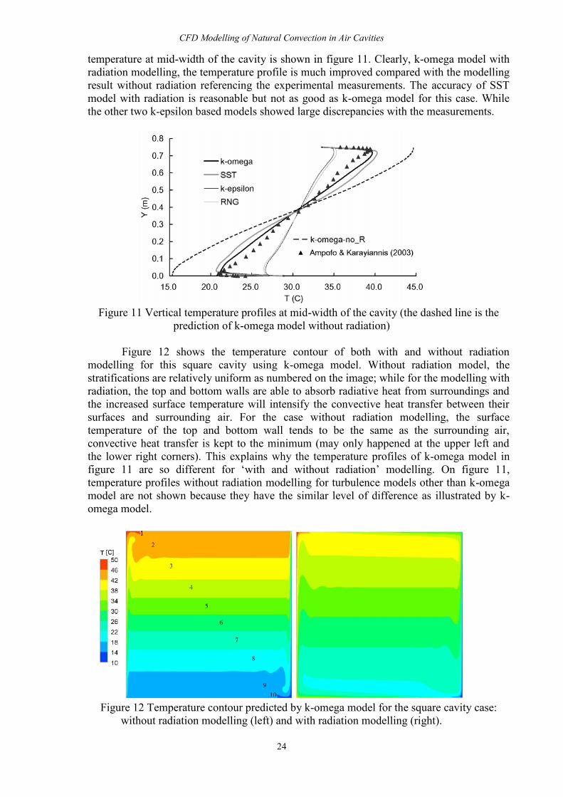
temperature at mid-width of the cavity is shown in figure 11. Clearly, k-omega model withradiation modelling, the temperature profile is much improved compared with the modellingresult without radiation referencing the experimental measurements. The accuracy of SSTmodel with radiation is reasonable but not as good as k-omega model for this case. Whilethe other two k-epsilon based models showed large discrepancies with the measurements.

Figure 11 Vertical temperature profiles at mid-width of the cavity (the dashed line is theprediction of k-omega model without radiation)

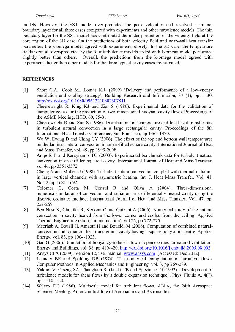
Figure 12 shows the temperature contour of both with and without radiationmodelling for this square cavity using k-omega model. Without radiation model, thestratifications are relatively uniform as numbered on the image; while for the modelling withradiation, the top and bottom walls are able to absorb radiative heat from surroundings andthe increased surface temperature will intensify the convective heat transfer between theirsurfaces and surrounding air. For the case without radiation modelling, the surfacetemperature of the top and bottom wall tends to be the same as the surrounding air,convective heat transfer is kept to the minimum (may only happened at the upper left andthe lower right corners). This explains why the temperature profiles of k-omega model infigure 11 are so different for ‘with and without radiation’ modelling. On figure 11,temperature profiles without radiation modelling for turbulence models other than k-omegamodel are not shown because they have the similar level of difference as illustrated by k-omega model.

Figure 12 Temperature contour predicted by k-omega model for the square cavity case:without radiation modelling (left) and with radiation modelling (right).


25

Figure 13 shows the mid-height vertical velocity profiles predicted by the fourturbulence models in comparison with the experimental measurements. The detailedmeasurements were conducted from the ‘hot’ wall side till the vertical velocity variationgets steady and close to zero. Both RNG and k-epsilon model failed to perform at theboundary inner layer and the predictions of the outer layer are poor, too. SST modelresolved the inner boundary similar as the k-omega model but had an overshoot of themaximum vertical velocity and consequently and relatively thinner outer boundary layercompared with both k-omega model and the measurements. Overall, k-omega modelperforms better here. Without the radiation model involved, all the models failed to predictthe boundary layer next to the hot wall. On figure 13, only k-omega model resulted profilewithout radiation is shown.

Figure 13 Vertical velocity profiles at mid-height close to the hot wall (the dashed line is theprediction of k-omega model without radiation)

Although the four turbulence models are using the same eddy viscosity assumption(Reynolds stresses are assumed to be proportional to mean velocity gradients) forrepresenting the turbulence viscosity t , the near wall treatments for these models aredifferent, which may have led to the differences of their predictions. The k-epsilon basedmodels use a ‘scalable wall function’ in which a lower limit for the first cell height close towall was set. This is the height at the intersection of the logarithmic and the linear near-wallprofile. In this approach the viscous sub-layer is bridged by employing empirical formulas toprovide near-wall boundary conditions for the mean flow and turbulence transportequations. Therefore all cells within the computing domain are outside the viscous sub-layerand this avoids the inconsistency caused by arbitrarily fine meshes. This wall function workswell for buoyancy-driven natural or forced convection in enclosed spaces when thebuoyancy turbulence is caused by localised heat sources [22, 23]. However, for the casesconsidered here, the buoyancy driving force is generated by the differentially heatedsurfaces. Parameters like wall heat transfer and shear stresses in the viscous sub-layer arevery sensitive with the near-wall formulation. It may not be appropriate using an empiricallogarithm profile outside the layer. The differences between the k-epsilon model and theRNG model are that the RNG model uses the renormalisation group analysis for the Navier-Stokes equations and also uses different model constants for the turbulence transportequations. The RNG model performs better than standard k-epsilon model when turbulencebuoyant plume is modelled [22-24].


26

The near-wall treatment for the k-omega based models is using the formulation forlow-Reynolds number computations. However, the k-omega models do not involve thecomplex non-linear damping functions required for the k-epsilon model and are thereforemore robust. The models allow for smooth shift from a low-Reynolds number form to a wallfunction formulation. The SST k-omega model gives highly accurate predictions of theonset and the amount of flow separation under adverse pressure gradients because itaccounts for the transport of the turbulent shear stress [15]. In this work, the airflow cavitydoes not involve the complicated flow structure like separation and reattachment. For thisreason the SST model did not offer more accurate prediction than the k-omega model of[14].

5.3 Three dimensional cavity predictions

Figure 14 shows the velocity and temperature predictions on the mid plane(y=0.25m) by k-omega turbulence model. There are about 10 to 12 cells to resolve theviscous sub-layer and this gives a smooth shift from the viscous layer to the turbulentregion. The maximum speed after the viscous layer is about 1.5m/s on the mid plane and thehighest (about 2.44m/s) speed is located close to the outlet of the cavity. This explains why asmaller first cell height is needed compared with the 2D case where the resulting air speednear wall was small. The thickness of the thermal boundary layer increases with height andtowards the top of the cavity the thermal boundary layers are interacting from one side to theother. This is also shown by the velocity profiles at locations (1, 2, 3) because the effectsfrom the boundary layer have propagated to the centre at the top of the cavity.

Figure 14 The velocity vectors and temperature contours on the symmetry plane (y=0.25).

Figure 15 shows the CFD predicted air velocity profiles at a height of 7.8mcompared with the experimental measurements [6]. The SST model predicted a higher meanvelocity at the boundary region. However, the effects of this high momentum are quickly


27

dissipated and do not seem to adequately affect the flow in the core of the cavity, where theair tends to be stagnant. Predictions from the other three models agreed with themeasurements in general with the k-omega model performed slightly better at both near-wallregion and the core flow. This is also true for the prediction of the temperature profile at thesame location (Figure 16).

The temperature profile predicted by the four turbulence models all follow the trendof the experiments but the predictions are all slightly higher than the measurements (Figure16). Again, the predictions of k-omega model are slightly closer to the experiments. Theover predictions of this temperature profiles may be caused by the relative portion of theradiative energy and the convective energy on the heated wall. A relative higher portion ofconvective heat was predicted by all four turbulence models (table 2) and this heat has beentaken away by air due to convection which may have increased the air temperature withinthe cavity. The mass flow rates predicted by CFD are all slightly smaller than that in [6]which may contribute another reason for the over-predictions of air temperature profile.

Figure 15 Comparisons between CFD and experiments for the prediction of velocity profilesat H =7.8m across the symmetry plane.

Figure 16 Comparisons between CFD and experiments for the prediction of air temperatureat H =7.8m across the symmetry plane.


28

Table 2 shows the comparisons between the experiments and the CFD predictionsfor 5 other parameters. The total heat flux is the overall heated wall energy output whichincluded both convective and radiative heat. When the heated wall is set to 150ºC themeasured total heat fluxes were tending to towards the lower band therefore all the CFDpredictions agreed with the measurements closely [6]. As discussed previously, allturbulence models predicted a slightly smaller ratio of radiative heat over convective heatcompared with experiments, which is also true for the predictions of the mass flow rate.This discrepancy may be caused by the radiation modelling where the radiative heat may beunder-predicted. The under-prediction of mass flow rate may be caused by loss coefficientimposed on the open ends, a smaller resistance than the current simulation setup may beneeded to overcome this. The CFD predicted local Nusselt numbers on the heated wall forconvective and total energy are also compared with the experiments. The predictions all fallin the range of the experimental measurements which indicates that all turbulence modelsperformed well with this parameter. However, there is a clear distinction between k-omegaand k-epsilon based models. The difference is considered to be caused by the near-walltreatment for these turbulence models, e.g. the scalable wall-function is used by the k-epsilon based models while the k-omega based models use automatic near-wall treatmentwhich automatically switches from wall-function to a low Reynolds number formulation atthe viscous sub-layer. Further discussions for these near-wall treatments and how theseNusselt numbers are calculated can be found in Appendix A.

TABLE 2 COMPARISONS BETWEEN TEHEXPERIMENTS AND CFD PREDICTIONS

Total heat fluxcr qq / Flow rate

cNu tNuMeasured 6.6010% (KW) 1.25 0.34 (kg/s) 112.210%k-epsilonmodel

6.24 (KW) 1.10 0.32 (kg/s) 132.2 277.6

RNG model 5.96 (KW) 1.16 0.30 (kg/s) 128.1 276.7SST model 6.04 (KW) 1.11 0.27 (kg/s) 102.9 217.1k-omegamodel

6.22 (KW) 1.14 0.32 (kg/s) 106.9 228.8

Key: rq , and cq are radiative, convective heat on the heated wall and cNu and tNu are the convective and totalNusselt Numbers which are defined in Appendix A.

6. Conclusion

This paper has demonstrated the ability of four widely eddy viscosity turbulence models formodelling natural convection airflow in closed and open ended cavities with and without radiation.Modelling techniques were detailed and the grid dependency was performed for all three cases.Simulation results have been compared with their corresponding experimental measurements. Thefour turbulence models performed differently when predicting key parameters of interest.

The k-epsilon based models resolved much lower peaks of mean velocity and kinetic energyat near-wall region for the 2D rectangular closed cavity case although the predictions of the coreregion agreed with experiments well. This is also true for the squared cavity with radiationmodelling in the prediction of the mid-height velocity. The two k-epsilon based models were notable to predict location of the transient onset, which is identified as the upper turning point for thelocal convective heat flux on the hot wall for the 2D rectangular case. When modelling the open-ended 3D case in conjunction with radiation k-epsilon based models performed better for theprediction of the near-wall velocity field and the heat transfer parameters compared with the 2Dcases. The k-omega based models were able to accurately predict the transient onset and resolvedhigher peaks of the mean velocity and kinetic energy for the rectangular 2D case. Similarly for thesquare 2D case with radiation, the k-omega based models performed better than the other two


29

models. However, the SST model over-predicted the peak velocities and resolved a thinnerboundary layer for all three cases compared with experiments and other turbulence models. The thinboundary layer for the SST model has contributed the under-prediction of the velocity field at thecore region of the 3D case. On the predictions of both velocity field and near-wall heat transferparameters the k-omega model agreed with experiments closely. In the 3D case, the temperaturefields were all over-predicted by the four turbulence models tested with k-omega model performedslightly better than others. Overall, the predictions from the k-omega model agreed withexperiments better than other models for the three typical cavity cases investigated.

REFERENCES

[1] Short C.A., Cook M., Lomas K.J. (2009) ‘Delivery and performance of a low-energyventilation and cooling strategy’, Building Research and Information, 37 (1), pp. 1-30.http://dx.doi.org/10.1080/09613210802607841

[2] Cheesewright R, King KJ and Ziai S (1986). Experimental data for the validation ofcomputer codes for the prediction of two-dimensional buoyant cavity flows. Proceedings ofthe ASME Meeting, HTD. 60, 75-81.

[3] Cheesewright R and Ziai S (1986). Distributions of temperature and local heat transfer ratein turbulent natural convection in a large rectangular cavity. Proceedings of the 8thInternational Heat Transfer Conference, San Fransisco, pp 1465-1470.

[4] Wu W, Ewing D and Ching CY (2006). The effect of the top and bottom wall temperatureson the laminar natural convection in an air-filled square cavity. International Journal of Heatand Mass Transfer, vol. 49, pp 1999-2008.

[5] Ampofo F and Karayiannis TG (2003). Experimental benchmark data for turbulent naturalconvection in an airfilled squared cavity. International Journal of Heat and Mass Transfer,vol 46, pp 3551-3572.

[6] Cheng X and Muller U (1998). Turbulent natural convection coupled with thermal radiationin large vertical channels with asymmetric heating. Int. J. Heat Mass Transfer. Vol. 41,No.12, pp.1681-1692.

[7] Colomer G, Costa M, Consul R and Oliva A (2004). Three-dimensionalnumericalsimulation of convection and radiation in a differentially heated cavity using thediscrete ordinates method. International Journal of Heat and Mass Transfer, Vol. 47, pp.257-269.

[8] Ben Nasr K, Chouikh R, Kerkeni C and Guizani A (2006). Numerical study of the naturalconvection in cavity heated from the lower corner and cooled from the ceiling. AppliedThermal Engineering (short communication), vol 26, pp 772-775.

[9] Mezrhab A, Bouali H, Amaoui H and Bouzidi M (2006). Computation of combined natural-convection and radiation heat transfer in a cavity having a square body at its centre. AppliedEnergy, vol. 83, pp 1004-1023.

[10] Gan G (2006). Simulation of buoyancy-induced flow in open cavities for natural ventilation.Energy and Buildings, vol. 38, pp 410-420. http://dx.doi.org/10.1016/j.enbuild.2005.08.002

[11] Ansys CFX (2009). Version 12, user manual, www.ansys.com [Accessed: Dec 2012][12] Launder BE and Spalding DB (1974). The numerical computation of turbulent flows.

Computer Methods in Applied Mechanics and Engineering, vol. 3, pp 269-289.[13] Yakhot V, Orszag SA, Thangham S, Gatski TB and Speziale CG (1992). “Development of

turbulence models for shear flows by a double expansion technique”, Phys. Fluids A, 4(7),pp. 1510-1520.

[14] Wilcox DC (1986). Multiscale model for turbulent flows. AIAA, the 24th AerospaceSciences Meeting. American Institute of Aeronautics and Astronautics.


30

[15] Menter FR (1994). Two-equation eddy-viscosity turbulence models for engineeringapplications. AIAA-Journal, vol. 32(8), pp 269-289.

[16] Stazi F., Mastrucci A. & Perna C. (2012). Trombe wall management in summer conditions:An experimental study, Solar Energy, Vol 86 (9), pp, 2839-2851.http://dx.doi.org/10.1016/j.solener.2012.06.025

[17] Rodríguez-Hidalgo M.C., Rodríguez-Aumente P.A., Lecuona A. & Nogueira J. (2012).Instantaneous performance of solar collectors for domestic hot water, heating and coolingapplications, Energy and Buildings, Vol 45, pp 152-160.http://dx.doi.org/10.1016/j.enbuild.2011.10.060

[18] Versteeg HK and Malalasekera W (1995). An introduction to computational fluid dynamics– the finite volume method. ISBN 0-582-21884-5.

[19] Ji Y, Cook MJ, Hanby VI, Infield DG, Loveday DL and Mei L (2007). CFD Modelling ofDouble-Skin Facades with Venetian Blinds. The 10th Int Building Performance SimulationAssociation Conf, 3-6 September, Beijing, China, pp. 1491-1498, ISBN: 0-9771706-2-4.

[20] Hsieh KJ and Lien FS (2004). Numerical modelling of buoyancy-driven turbulent flows inenclosures. International Journal of Heat and Fluid Flow, Vol. 25, pp. 659-679..

[21] Bowles A and Cheesewright R (1989). Direct measurement of the turbulence heat flux in alarge rectangular air cavity. Experimental Heat Transfer, Vol. 2, pp. 59-69.

[22] Cook MJ, Ji Y and Hunt GR (2003). CFD modelling of natural ventilation: combined windand buoyancy forces. International Journal of Ventilation, Vol. 1, pp. 169-180.

[23] Ji Y, Cook MJ and Hanby V (2007). Modelling of displacement natural ventilation in anenclosure connected to an atrium. Building and Environment, vol. 42, pp 1158-1172.http://dx.doi.org/10.1016/j.buildenv.2005.11.002

[24] Chen Q (1995). Comparison of different k- models for indoor air flow computations.Numerical Heat Transfer, Part B, vol. 28, pp 353-369.

Appendix A: Nusselt Numbers on the heated wall for the 3D cavity

The measurement of local convective Nusselt number was correlated by the following equation:3/11.0 RaNuc (A1)

where, the Rayleigh number Ra is defined by equation A2)/()( 3 TglRa (A2)

The parameters at the average temperatures 30C for equation A2 are shown in table A1 andthese properties gave a Ra number as 1.41109.

TABLE A1 PARAMETERS FOR EQUATION A2

expansioncoefficient

(1/K)

Gravity g(m/s2)

Characteristiclength l (m)

Temperaturedifference

T (K)

Kinematicviscosity

(m2/s)

Thermaldiffusivity

(m2/s)0.00330 9.81 0.5 130.0 1.60 10-5 2.29 10-5

The total Nusselt number was defined by crct qqNuNu /1 (A3)

where rq and cq are the radiative and convective heat fluxes on the heated wall, which can becomputed from the CFD directly.The local convective Nusselt number at the heated wall in CFD can be defined by equation A4

cNu =T

lyT )/( (A4)


31

where yT / is the temperature gradient related to the near-wall treatments for differentturbulence models. In this work, T is treated as the difference between the CFD calculatednear-wall temperature and the boundary temperature, and y is the normal distance from theheated wall where this near-wall temperature is calculated.The key advantage of using scalable wall-function in the k-epsilon based models is to set alower y (dimensionless wall distance) limit as the intersection between the logarithmic and thelinear near-wall profile which will avoid the mesh sensitivity close to the wall [11]. In this work,this limit is 11.6 because the meshes used have much smaller averaged y values across theheated wall. Therefore the actual distance ( y ) between the heated wall and the intersectionpoint can be obtained by the following equation:

/)( * yuy =11.6 (A5)where *u is the near-wall velocity defined by

2/14/1* kCu (A6)where k is the kinetic energy which can be computed by CFD, C is the model constant (RNGmodel C =0.085 and k-epsilon model C =0.09)For k-omega based turbulence models, the automatic near-wall treatment was used. The near-wall temperature was calculated at the first cell height therefore y is the physical height of thefirst cell next to the heated wall.The CFD computed T and y values used to calculated local convective Nusselt number aresummarised in the following table A2

TABLE A2 T AND y VALUES CALCULATED BY THE TURBULENCE MODELS

T (K) y = y (mm)k-omega 6.945 0.25

SST 6.689 0.25k-epsilon 68.73 2.0

RNG 66.63 2.04

cfd modelling of natural convection in air cavitiesusir.salford.ac.uk/35008/1/347-1300-1-pb.pdf ·...

Documents