MOL.20021224.0115

SAND REPORT SAN D2002-3 1 32 Unlimited Release Printed October 2002

CFD Calculation of Internal Natural Convection in the Annulus between Horizontal Concentric Cylinders

Nicholas D. Francis, Jr., Michael T. Itamura, Stephen W. Webb, and Darryl L. James

Prepared by Sandia National Laboratories Albuquerque, New Mexico 871 85 and Livermore, California 94550

Sandia is a multiprogram laboratory operated by Sandia Corporation, a Lockheed Martin Company, for the United States Department of Energy under Contract DE-AC04-94AL85000.

Approved for public release; further dissemination unlimited.

@ Sandia National laboratories

Issued by Sandia National Laboratories, operated for the United States Department of Energy by Sandia Corporation.

NOTICE: This report was prepared as an account of work sponsored by an agency of the United States Government. Neither the United States Government, nor any agency thereof, nor any of their employees, nor any of their contractors, subcontractors, or their employees, make any warranty, express or implied, or assume any legal liability or responsibility for the accuracy, completeness, or usefulness of any information, apparatus, product, or process disclosed, or represent that its use would not infringe privately owned rights. Reference herein to any specific commercial product, process, or service by trade name, trademark, manufacturer, or otherwise, does not necessarily constitute or imply its endorsement, recommendation, or favoring by the United States Government, any agency thereof, or any of their contractors or subcontractors. The views and opinions expressed herein do not necessarily state or reflect those of the United States Government, any agency thereof, or any of their contractors.

Printed in the United States of America. This report has been reproduced directly from the best available copy.

Available to DOE and DOE contractors from U.S. Department of Energy Ofice of Scientific and Technical Information P.O. Box 62 Oak Ridge, T N 3783 I

Telephone: (865)576-840 1 Facsimile: (865)576-5728 E-Mail: reports@,adonis.osti.gov Online ordering: http://www.doe.aovlbridee

Available to the public from U.S. Department of Commerce National Technical Information Service 5285 Port Royal Rd Springfield, VA 22161

Telephone: (800)553-6847 Facsimile: (703)605-6900 E-Mail: ordersmntis. fedworld. go v Online order: htto://www.ntis.aov/hel~/orde~ethods.asu?~oc=7-4-O#on line

2

-4

SAND2002-3 132 Unlimited Release

Printed October 2002

CFD Calculation of Internal Natural Convection in the Annulus between Ho rizo n t a1 Concentric Cylinders

Nicholas D. Francis, Jr., and Michael T. Itamura Subsystems Performance Assessment Department

Stephen W. Webb Environmental Technology Department

Sandia National Laboratories P.O. Box 5800

Albuquerque, NM 871 85-0776

Darryl L. James Texas Tech University

Department of Mechanical Engineering Box 41021

Lubbock, TX 79409- 102 1

ABSTRACT

- -

The objective of this heat transfer and fluid flow study is to assess the ability of a computational fluid dynamics (CFD) code to reproduce the experimental results, numerical simulation results, and heat transfer correlation equations developed in the literature for natural convection heat transfer within the annulus of horizontal concentric cylinders. In the literature, a variety of heat transfer expressions have been developed to compute average equivalent thermal conductivities. However, the expressions have been primarily developed for very small inner and outer cylinder radii and gap-widths. In this comparative study, interest is primarily focused on large gap widths (on the order of half meter or greater) and large radius ratios. From the steady-state CFD analysis it is found that the concentric cylinder models for the larger geometries compare favorably to the results of the Kuehn and Goldstein correlations in the Rayleigh number range of about 1 O5 to 10' (a range that encompasses the laminar to turbulent transition). For Rayleigh numbers greater than 1 Os, both numerical simulations and experimental data (from the literature) are consistent and result in slightly lower equivalent thermal conductivities than those obtained from the Kuehn and Goldstein correlations.

3

CONTENTS

1 INTRODUCTION ................................................................................................................... 11

2 MODEL DESCRIPTION AND COMPARISON TO LITERATURE DATA AND RESULTS ...................................................................................................................................... 11

2.1 Introduction ..................................................................................................................... 12

2.2 Turbulence Modeling ...................................................................................................... 14

2.3 Literature Results for Natural Convection in an Annulus .............................................. 18

2.4 CFD Models Developed to Compare to Literature Results ............................................ 21

2.5 Grid Specifications for Concentric Cylinders ................................................................. 21

2.6 CFD Model Settings and Parameters .............................................................................. 23 2.7 Boundary Conditions ...................................................................................................... 25

2.8 Thermal Properties .......................................................................................................... 25

2.9 Operating Conditions ...................................................................................................... 27

2.10 Results of the Comparative Heat Transfer Study ............................................................ 28 2.10.1 Appropriateness of the Turbulence Model used in the Study ....................... 28 2.10.2 Correlation, Experimental Data, and CFD Code Comparison for Average Heat Transfer .................................................................................................................. 30 2.10.3 Experimental Data and CFD Comparison for Local Heat Transfer .............. 33 2.10.4 Experimental Data and CFD Comparison for Local Temperature ................ 34 2.10.5 Grid Independence Study .............................................................................. 36

3 DISCUSSION .......................................................................................................................... 39

4 REFERENCES ........................................................................................................................ 39

- . -

4

Figure 1.

Figure 2.

Figure 3.

Figure 4.

Figure 5 .

Figure 6.

Figure 7.

Figure 8.

-9

FIGURES Page

Computational Grid for the 25%-Scale Concentric Cylinder Geometry.. .................. .23

Turbulent Reynolds Number for Full-scale Concentric Cylinders (RUL = 5.3~10 ). ....................................................................................................................... 29 9

Comparison of CFD Model Results to the Kuehn and Goldstein Correlation Equation (1 978) and the General Correlation in Kuehn and Goldstein (1 976b) for Concentric Cylinders. ........................................................................................... ..30

Comparison of CFD Model Results for Concentric Cylinders to Other Experimental Results, Model Results, and Heat Transfer Correlations ...................... 32

Comparison of Local CFD Model Heat Transfer to the Kuehn and Goldstein (1 978) Experimental Measurements for Pressurized Nitrogen (Concentric Cylinders). ................................................................................................................... .34 - -

Comparison of CFD Model Temperatures to the Kuehn and Goldstein (1 978) Experimental Measurements for Pressurized Nitrogen (Concentric Cylinders) .......... 35

Refined Grid (8 1x8 1) for the Full-scale Concentric Cylinders ................................... 37

Centerline Vertical Velocity for the Full-scale Concentric Cylinders ...................... ..3 8

5

Table 1.

Table 2.

Table 3.

Table 4.

Interns

TABLES

Page

Natural Convection Heat Transfer in the Literature ....................................... 13

Concentric Cylinder Geometries.. ............................................................................... .2 1

Operating Conditions .................................................................................................. .27

Grid Independence Study for Heat Transfer Rates .................................................... .3 7

6

NOMENCLATURE

empirical constant (9.8 1) fluid specific heat (J/kg-K) RNG theory determined constant (0.0845) inner cylinder wall diameter (m) outer cylinder wall diameter (m) total energy (J/kg) acceleration due to gravity (m/s2) mean overall heat transfer coefficient ( W/m2-K) average equivalent thermal conductivity for natural convection (-) turbulent kinetic energy (m2/s2) turbulent kinetic energy at wall adjacent cell center (m2/s2) air thermal conductivity (W/m-K) annulus gap width, R, - Ri (m) molecular weight of air (kg/kmol) Nusselt number for natural convection from the inner cylinder (-) Nusselt number for natural convection from the outer cylinder (-) average overall Nusselt nuEber -

NUcond Nusselt number for conduction Nuc,, Nusselt number for convection between concentric cylinders P pressure m/m2> Pr Prandtl number (-) Pr, turbulent Prandtl number (-)

Qcond q "

total heat transfer rate from the CFD models (W) conduction heat transfer rate from the CFD models (W) wall heat flux (W/m2)

r*

AT E

R - Ri L

dimensionless radial distance, -

universal gas constant (N-dkmol-K) turbulent Reynolds number (-) Rayleigh number based on gap-width (-) Rayleigh number based on inner diameter (-) Rayleigh number based on outer diameter (-) radial distance (m) outside radius (m) inside radius (m) inner cylinder wall temperature (K or "C) outer cylinder wall temperature (K or "C) cold cylinder (outer) wall temperature (K or "C) hot cylinder (inner) wall temperature (K or "C) inner cylinder film temperature based on bulk temperature outer cylinder film temperature based on bulk temperature temperature difference (K or "C) bulk fluid temperature (K or "C)

7

Tp T, U velocity ( d s ) Y yp

fluid temperature at wall adjacent cell center (K or "C) wall temperature (K or "C)

normal distance to nearest wall (m) distance from wall adjacent cell center to the wall (m)

Greek

fluid thermal diffusivity, k J p , (m2/s), inverse effective Prandtl numbers volumetric thermal expansion coefficient (IC') laminar thermal boundary layer thickness for a plane wall (m) laminar viscous boundary layer thickness for a plane wall (m) dissipation rate of turbulent kinetic energy (m2/s3) angular position (0" vertical up, 180' vertical down) molecular fluid viscosity (kg/m-s) turbulent viscosity (kg/m-s) effective viscosity, ,ut + ,u (kg/m-s) fluid kinematic viscosity, ,dp (m2/s) fluid density (kg/m3) wall shear stress (N/m2)

- -

*I

V viscosity ratio,

T - T, dimensionless temperature, - (-)

Th -Tc 4 w specific dissipation rate

8

ACKNOWLEDGEMENTS

The authors would like to thank Charles E. Hickox, Jr., of Sandia National Laboratories and Veraun Chipman of Lawrence Livermore National Laboratory for their thorough reviews of this document. This work was supported by the Yucca Mountain Site Characterization Office as part of the Office of Civilian Radioactive Waste Management (OCRWM), which is managed by the U.S. Department of Energy, Yucca Mountain Site Characterization Project. Sandia is a multiprogram laboratory operated by Sandia Corporation, a Lockheed Martin Company, for the United States Department of Energy under Contract DE-AC04-94AL85000.

9

Intentionally Left Blank

10

1 INTRODUCTION

This report documents a comparison of computational fluid dynamics (CFD) simulations of natural convection in the annulus formed between horizontal concentric cylinders with experimental data and other numerical simulations available in the heat transfer literature. CFD simulations are used to compute both overall and local heat transfer rates for concentric cylinder arrangements. The CFD calculated heat transfer rates are then used directly in comparisons with data, correlation equations, and other numerical simulations. In this comparative study, interest is primarily focused on large gap widths (on the order of 0.5 m or greater) with radius ratios (RJRJ of about 3.5.

Although the Yucca Mountain Project (YMP) geometries are not concentric, a typical simplifying assumption is made such that an average equivalent thermal conductivity for natural convection can be computed with an existing correlation applied at a geometric scale appropriate to YMP. The resulting average equivalent thermal conductivity is then applied to a non-concentric annulus. This report focuses on heat transfer and fluid flow within the annulus between horizontal concentric cylinders at the scale appropriate to YMP. Francis et al., 2002, develops an analysis of heat transfer and fluid flow within the annulus of non-concentric cylinders.

The CFD computer code, FLUENT, version 5.5 (Fluent Incorporated, 1998) and version 6.0 (Fluent Incorporated, 2001), are used for the analysis. FLUENT is a computational fluid dynamics code that solves conservation of mass, momentum, energy (including a radiative transfer equation), species, and turbulence models using various means to obtain closure for the turbulent momentum equations. Transient or steady state formulations are also available. For this heat transfer analysis, both steady-state laminar and turbulent natural convection heat transfer are considered.

2 MODEL DESCRIPTION AND COMPARISON TO LITERATURE DATA AND RESULTS

This section provides a brief discussion of previous natural convection heat transfer experiments, correlation equations, and numerical simulations. In the literature, a variety of heat transfer expressions have been developed for horizontal concentric cylinders. However, these expressions are typically based on experimental results using very small inner and outer cylinder radii (on the order of a few centimeters) and gap-widths (1.9 cm I L I 7.1 cm). In the present natural convection heat transfer study, the correlation equations are applied to much larger gap-widths (0.5 m I L 5 1.9 m) and cylinder radii (0.2 m 2 Ri, R, 5 2.75 m).

-%

11

2.1 Introduction

This report considers the effects of an imposed temperature difference and system geometry on CFD calculations of internal natural convection heat transfer in a horizontal annulus. Comparisons to established heat transfer correlation equations and experimental heat transfer measurements described in the literature are performed. An investigation of this type provides an evaluation of the capability of the CFD code to predict heat transfer in a known geometry as a precursor to calculating conditions in modified configurations.

Previous experimental and theoretical studies of internal natural convection in the annulus between horizontal cylinders have been largely restricted to simple geometries such as concentric or eccentric horizontal cylinders. In many of these cases, the geometries have small (- 3 cm) gap widths (L = R, - Ri). Typically, a single radius ratio was considered (e.g., Kuehn and Goldstein, 1976a and 1978, considered a radius ratio of 2.6; Bishop, 1988, and McLeod and Bishop, 1989, considered a radius ratio of 3.37; Vafai et al., 1997, considered a radius ratio of 1.1). A limited number of numerical and experimental studies have investigated the influence of the radius ratio on internal flow characteristics (Lis, 1966; Bishop et al, 1968; Desai and Vafai, 1994; Char and Hsu, 1998). Some investigators developed heat transfer correlation equations for their experimental results (Lis, 1966; Bishop et al, 1968; Kuehn and Goldstein, 1976a; Kuehn and Goldstein, 1978; Bishop, 1988). In the experimental studies, the range of radius ratios considered was 1.1 5 RJRi 5 4. In the numerical studies, a wide range of radius ratios was considered (1.5 I: ROIRi 5 1 l), including a radius ratio of 3.5, which is similar to that of the Yucca Mountain Project (YMP) geometry (Webb et al., 2002). In the present comparative study, interest is focused on large gap widths (on the order of 0.5 m or greater) and larger radius ratios (ROIRi 3.2-3.5) than used in most of the experimental studies.

Most of the concentric cylinder modeling studies consider gases (Pr =: 0.7) as the working fluid in the annulus (Kuehn and Goldstein, 1976a; Kuehn and Goldstein, 1978; Farouk and Guceri, 1982; Desai and Vafai, 1994); although, some investigated a larger range of Prandtl numbers (Kuehn and Goldstein, 1976a; Desai and Vafai, 1994). An experimental analysis used water (Pr = 5 ) as the working fluid in the annulus (Kuehn and Goldstein, 1976a). Some numerical studies considered Prandtl numbers as high as 5000 (engine oil at room temperature) and as low as about 0.01 (liquid metals). The present study considers gases with a Prandtl number of approximately 0.7 (e.g., air, nitrogen).

Table 1 lists the investigators and the form in which their natural convection heat transfer investigation was presented (experiment, correlation equation, and numerical simulations).

12

-4

Webb et al., 2002

Table I. Internal Natural Convection Heat Transfer in the Literature

X X - -

For internal natural convection in an annulus, a Rayleigh number based on gap-width

gPATL3 Ra, = V f f

is normally used to determine if the internal flow is laminar or turbulent (Kuehn and Goldstein, 1978). The transition gap-width Rayleigh number for turbulence is about 1 O6 (Kuehn and Goldstein, 1978; Desai and Vafai, 1994; Char and Hsu, 1998). For Rayleigh numbers less than 1 06, the flow is laminar.

For Rayleigh numbers greater than the transition value, the annulus internal flow conditions are characterized by a turbulent upward moving plume above the inner cylinder and a turbulent downward flow against the outer wall. Stagnation regions exist near the top where the plume impinges on the outer cylinder and over the entire bottom of the annulus. A low velocity laminar region exists in the annulus away from the walls. Turbulent flow conditions in the annulus are typically obtained either through the length scale (e.g., gap width) or the operating conditions (e.g., temperature difference and operating pressure) of the configuration. For the very small gap widths (- 3 cm) considered in the experiments presented in the literature, air at atmospheric temperatures and pressures would not result in turbulent flow (e.g., RaL < lo6). Pressurized gases such as nitrogen were often used in experiments to obtain the fluid properties necessary to achieve turbulent Rayleigh numbers for very small gap widths and small temperature differences (Kuehn and Goldstein, 1978). The results of the experiments were then used

13

to establish correlation equations that relate fluid properties and apparatus geometry to average heat transfer rates, as discussed in an upcoming section. Numerical simulations have been developed for some of the experimental geometries to compare model predictions to measured temperatures and heat transfer coefficients. Most of the numerical simulations are two-dimensional, but a limited number of three-dimensional studies have been conducted (Fusegi and Farouk, 1986; Desai and Vafai, 1994).

Most of the experimental data discussed above and presented in the literature are restricted to heat transfer results such as temperature and equivalent thermal conductivity. Experimental measurements of fluid velocity and turbulence quantities for the annulus configuration have not been published in the literature.

In the present study, a variety of two-dimensional models are developed to compare directly to the existing heat transfer correlations and experimental data developed in the literature. The two-dimensional CFD models are applied for both laminar and turbulent flow Rayleigh numbers.

2.2 Turbulence Modeling - -

Turbulence is characterized by fluctuating quantities (e.g., velocity, temperature, etc.). The velocity fluctuations impact transport of quantities such as mass, momentum, and energy. Direct simulation of all scales of a velocity fluctuation is not computationally practical. Therefore, simplifications for turbulent flow solutions are necessary. Typical approaches for handling turbulent flows are through Reynolds averaging or filtering the Navier-Stokes equations. However, both methods introduce unknown terms into the Navier-Stokes equations; therefore, additional turbulence modeling is required to achieve closure of the flow equations.

Reynolds-averaged Navier-Stokes equations (RANS) are written in terms of mean quantities and unknown terms with respect to the time-averaged fluctuating components that are generally referred to as the turbulent Reynolds stresses. The RANS approach is used in the following turbulence models available in FLUENT:

,

One equation model:

0 Spalart- Allmaras

Two equation models:

k-E models including, standard, realizable, and renormalization-group (RNG) k-w models including, standard and shear-stress transport

Five equation model (in two-dimensions) and a seven equation model (in three- dimensions)

14 .

-3

0 Reynolds stress model (RSM)

Filtered Navier-Stokes equations typically remove eddies Lat are smaller than the computational mesh size. Larger eddies are fully computed in a time-dependent simulation of the flow. Similar to the Reynolds-averaging, filtering also introduces unknown terms in the Navier-Stokes equations. These terms are related to the subgrid- scale stresses. Additional turbulence modeling is necessary to achieve closure. The filtering approach is used in the following turbulence model in FLUENT:

0 Large eddy simulation (LES)

Due to computational limitations associated with the time-dependent approach of the LES, the CFD analyses described in this document utilize the RANS equations (specifically the RNG k-E turbulence equations).

In the RANS approach, unsteadiness is removed by casting all variables (e.g., velocity, temperature, and pressure) into mean and fluctuating components and time-averaging the subsequent governing equations. The governing flow equations, written in terms of mean velocity and temperature components, for mass, momentum, and energy take the following forms after averaging:

Conservation of Mass (Continuity)

aP a at axi - + - ( p y ) = 0

Conservation of Momentum wavier-Stokes)

at

(3) All of the terms in equation (3), with the exception of the last term, are written with respect to mean velocities or pressure. The last term on the RHS of the momentum equation contains the turbulent Reynolds stresses.

Conservation of Energy

where viscous heating and source terms .are neglected and ite# = afipfi@ The CZT term is computed in a manner similar to the inverse effective Prandtl numbers in the turbulence

15

equations described below. The turbulent Prandtl number for energy is a function of the molecular Prandtl number and the effective viscosity described below.

The Boussinesq hypothesis (an assumption applied by the Spallart-Allmaras, k-E, and k-w turbulence models) can be used to relate the Reynolds stresses to the mean velocity gradients and other turbulence quantities including the turbulent viscosity:

As described above, a number of different turbulence models can be applied when solving turbulent flow fields. The RNG k - E is selected for this analysis. The primary reasons for using the RNG k - E turbulence model are that it allows for variation in the turbulent Prandtl number as a function of flow conditions, it provides a means for including low-Reynolds number effects in the effective viscosity formulation, and it includes an extra term, RE, in the &-equation to better model separated flows. The conservation equations for the RNG k-E turbulence (two-equation) model are given below:

- - k - turbulent kinetic energy

E- dissipation of turbulent kinetic energy

(7) where f f k and aE are inverse effective Prandtl numbers derived analytically by the RNG theory, Gk is the generation of turbulent kinetic energy due to mean velocity gradients, Gh is the generation of turbulent kinetic energy due to buoyancy (a function of gravity and temperature gradient), YM is the contribution of fluctuating dilation to the dissipation rate, CIE and c2E are constants, c3E is a (calculated) factor related to how the buoyant shear layer is aligned with gravity, and RE is a strain rate term written as a function of the mean rate-ofdrain tensor. Including full buoyancy effects in the equations is related to inclusion of the generation of turbulence due to a buoyancy term in the transport equation for the dissipation rate of turbulent kinetic energy (e.g., in the &-equation). In the governing equations, the subscripts i , j , and I refer to values in the various directions (i = x, y , and z directions;j = x, y, and z directions, I = x, y , and z directions).

The RNG k - E turbulence model provides an analytically derived differential formula for the effective viscosity that accounts for low-Reynolds number effects in the flow domain. It is written in terms of the effective viscosity, b@

d[ -1 P2k = 1.72 d- li dli dz l i3 -1 + C”

where 6 = ’% and C, is a constant (~100) . The differential equation for viscosity is

applicable to low-Reynolds number and near-wall flows. In the high Reynolds number limit, the turbulent viscosity produced by the differential equation is given by:

The various model constants are C1, = 1.42, C2, = 1.68, and C, = 0.0845, which are the default values in FLUENT. For complete details, refer to the FLUENT documentation on modeling turbulence (Fluent, Inc., 2001).

Use of the differential formula for the viscosity requires an appropriate treatment of the near-wall region. Specifically, it requires that the viscous sublayer and the buffer layer (e.g., the near-wall region) are resolved (meshed) all the way to the wall (e.g., to the surface of the inner and outer cylinders). The use of hydrodynamic wall functions (e.g., an alternative approach using semi-empirical modeling of the near-wall velocity behavior) is not appropriate when low-Reynolds number effects are pervasive within the flow domain. Additionally, the hydrodynamic wall function approach is not applicable in the presence of strong body forces (as in the case of buoyancy-driven flows). The inapplicability of the hydrodynamic wall function approach is illustrated in Figure 4 of this document. As shown in the figure, Desai and Vafai, 1994, apply standard wall functions through the viscous sublayer in their analysis of internal natural convection. Their resulting heat transfer rates tend to underpredict the other literature results. Therefore, the boundary layer must be adequately resolved by the grid in order to obtain the correct surface heat transfer rates (the quantity used to determine the heat transfer characteristics previously described).

A wall function approach is used for the near-wall mean temperature. In the viscous sublayer, a linear law is written in terms of the molecular Prandtl number:

T * = P r y * (y* c y ; )

while in the turbulent sublayer, a logarithmic law is written in terms of the turbulent Prandtl number:

17

I I

L J

where K is von Karman's constant (0.41) and P is a function of the molecular and turbulent Prandtl numbers (Fluent Incorporated, 200 1). The dimensionless quantities in the above equations are defined as:

and,

4"

Y Y * PCP4kP2YP

Y = P

- -

The selection of linear or logarithmic laws is based on the computation of y;. This quantity is computed as the y* value at which the linear law and the logarithmic law

intersect. For a refined grid (e.g., y' = 2 <lo), the linear law (equation 10) is ' : J P selected based on the intersection of the two curves. It is noted that in equilibrium turbulent boundary layers, y* and yf are approximately equal. The law-of-the-wall for temperature is acceptable in this analysis since the near-wall treatment for velocity places grid points inside the viscous sublayer. Subsequently, the natural convection boundary layer is resolved for both velocity and temperature.

2.3 Literature Results for Natural Convection in an Annulus

Numerous investigators (refer to Table 1) have developed natural convection heat transfer correlations for horizontal concentric and eccentric cylinders that relate an average equivalent thermal conductivity in an annulus to Rayleigh numbers based on the inner and outer diameters. The average equivalent thermal conductivity is defined as the ratio of natural convection heat transfer to that of pure conduction. An equivalent thermal conductivity of one is representative of pure conduction heat transfer. The equivalent conductivity indicates the importance of natural convection when compared to pure conduction.

The analysis in this section focuses on the correlation equations developed by Kuehn and Goldstein. The general heat transfer correlation developed by Kuehn and Goldstein

18

(1976b) is valid for any Prandtl number and for laminar or turbulent internal flow conditions. The heat transfer correlation in Kuehn and Goldstein (1978) is valid for a Prandtl number of about 0.7 (applicable to pressurized nitrogen which was the working fluid used in their work) and for laminar or turbulent flow conditions. Kuehn and Goldstein (1 978) made modifications to the empirical constants in the general correlation thereby making it somewhat more specific to the experimental geometry and conditions as described in that paper (e.g., RJRi = 2.6 and 2x102 < RaL < 8 ~ 1 0 ~ ) . The correlation presented in Kuehn and Goldstein (1978) is described below by equations (14) through (22). The more general correlation presented in Kuehn and Goldstein (1976b) is not discussed in detail here due to its complexity; however, it is shown graphically in the various comparisons between correlations and models. Note that the Kuehn and Goldstein (1978) correlation equation is one of the most widely used correlations for natural convection heat transfer in a horizontal annulus. For example, Gebhart et al., 1988; Bejan, 1995, and Incropera and DeWitt, 1990, all recommend use of the Kuehn and Goldstein heat transfer correlation equations for natural convection in an annulus.

The Kuehn and Goldstein (1 978) heat transfer correlation equations described below are functions of fluid properties, annulus geometry, temperature difference, and a bulk fluid temperature. The correlation is based on Rayleigh numbers for the inner and outer cylinders and a bulk fluid temperature as:

and,

The fluid properties in equations (14) and (15) are evaluated at the film temperature written as a function of the bulk temperature, that is, for the inner cylinder,

'Tj,ff,-i = ( T B +T.) I / , and for the outer cylinder, T~[,-, = 6 +T~x. The bulk fluid

temperature is defined by Kuehn and Goldstein as:

0 - Nui -

r , - T -To Nui + N U ,

where the Nusselt numbers in equation (16) are based on the inner and outer cylinder Rayleigh numbers and are defined as:

19

2

r 1 Nuj =

2 "1 i- [(O.SRa,,x 1' + (0.12RaD,X 1 and,

-2

r 1 2

[ (Ra,,% 1' + (0: 12RaD,%

Equations (17) and (1 8) are valid for a Prandtl number of 0.7 and any Rayleigh number. The average equivalent thermal conductivity for natural convection is defined as the following:

The Nusselt number parameters in equation ( 1 9) are defined as:

, concentric cylinders only 2

In ~

NVcond = - D O

4 Nu = [(Nu,,,)" NU,,,,,,^^^

and the convection Nusselt number is:

- 1

Nu,,,, = [I + 1 1 Nui Nu,

where inner and outer cylinder Nusselt numbers NUi and Nu, are from equations (1 7) and (IS), respectively. The conduction Nusselt number (equation 20) is specifically derived for concentric cylinders. Solution of the above equations requires an initial guess for the bulk fluid temperature, E. Typically, about 4 to 5 iterations are required to obtain convergence to within a fraction of a percent. Upon convergence, equation (19) gives the average equivalent thermal conductivity.

The comparison with the Kuehn and Goldstein heat transfer correlations (1976b and 1978) is selected in this report since these correlations are widely considered standards in

20

the natural convection heat transfer literature. However, other annulus heat transfer correlation equations exist in the literature. Some of the more recent are Bishop (1988) and McLeod and Bishop (1989), who provided an equation for the average equivalent conductivity in terms of Rayleigh number based on gap width and expansion number @IT). Lis (1966) provided an equation for the average equivalent conductivity in terms of Rayleigh number based on diameter and other geometrically based terms. Raithby and Hollands (1 975) provided an equation for the average equivalent conductivity in terms of the Prandtl number, a Rayleigh number based on gap width, and other geometric based terms. Finally, Vafai et al. (1997) provide for an average Nusselt number correlation in terms. of a modified Rayleigh number.

Case

Kuehn and Goldstein, 1978

25%-Scale YMP

2.4 CFD Models Developed to Compare to Literature Results

Inner Cylinder, Outer Cylinder, DdD, Gap-W idth

0.0356 0.0926 2.6 0.03

0.4 1.37 3.4 0.5

0, (m) Do 0-4 L (m)

A number of two-dimensional CFD models were developed to compare to the existing literature results and correlation equations applied to YMP-scale geometries. Concentric cylinder models for 25%-scale, 44%-scale, and full-scale geometries are compared to the correlation equations. Additionally, a two-dimensional CFD model is developed based on Kuehn and Goldstein’s experimental geometry and operating conditions (Kuehn and Goldstein, 1978, RaL = 2 . 5 1 ~ 1 0 ~ ) and is compared directly to their correlation equation.

2.5 Grid Specifications for Concentric Cylinders

The geometric specifications for the horizontal concentric cylinder CFD simulations are given in Table 2. The table includes the modeled case, inner and outer cylinder diameters, diameter ratio (radius ratio), and the gap width. The significant difference in the scales between previous experiments and the application to YMP is clearly shown in Table 2.

144%-ScaleYMP I 0.7 I 2.42 I 3.5 ~ 1.9

I Full-Scale YMP I 1.7 I 5.5 1 3.2 I 1.9

The radial and angular discretization for the large-scale geometries (25%-scale, 44%- scale, and full-scale) is described below. In the case of 25%-scale and full-scale geometries, the radial discretization included 61 divisions. In the case of the 44%-scale geometry, the radial discretization included 50 divisions. In each of the large-scale geometries, the radial divisions included cell clustering at the walls of both the inner and outer cylinders (refer to Figure 1). A two-sided cell clustering factor (e.g., refinement on

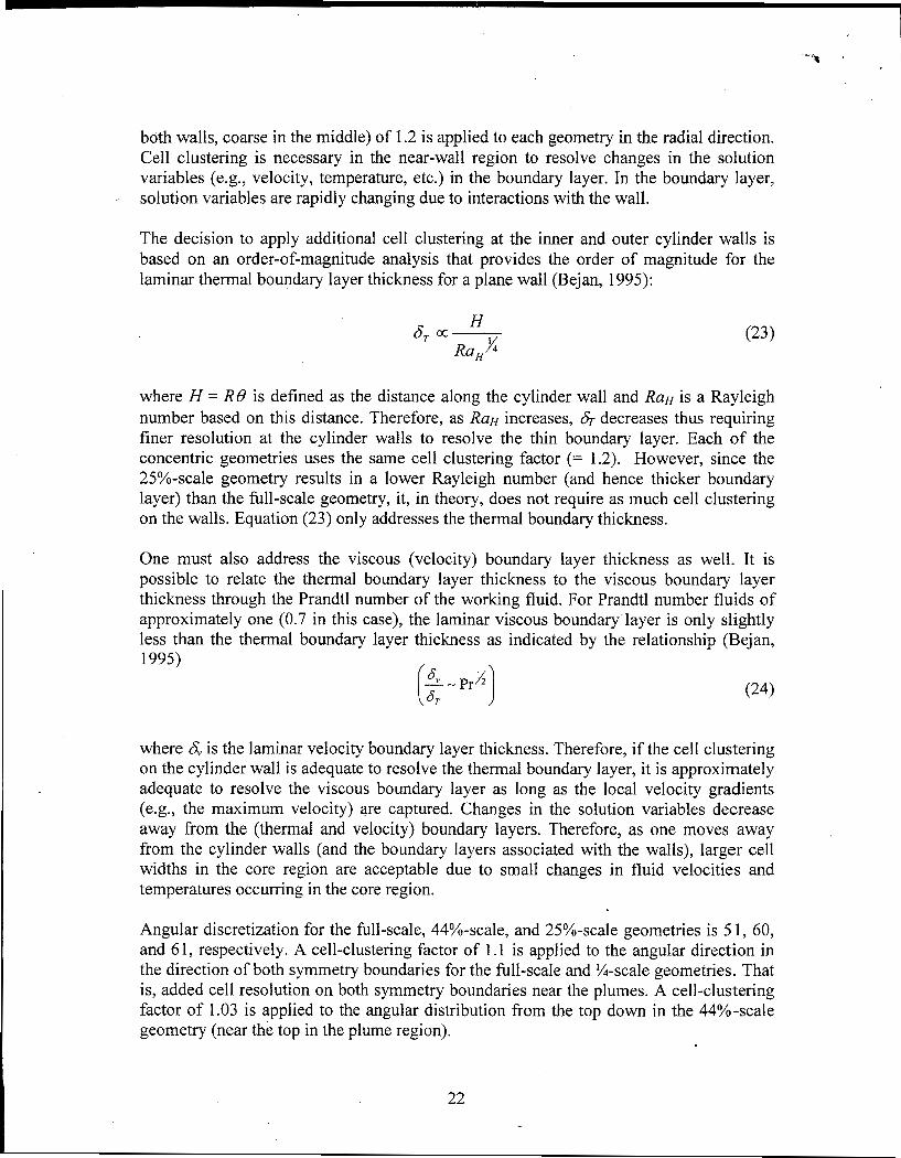
both walls, coarse in the middle) of 1.2 is applied to each geometry in the radial direction. Cell clustering is necessary in the near-wall region to resolve changes in the solution variables (e.g., velocity, temperature, etc.) in the boundary layer. In the boundary layer, solution variables are rapidly changing due to interactions with the wall.

The decision to apply additional cell clustering at the inner and outer cylinder walls is based on an order-of-magnitude analysis that provides the order of magnitude for the laminar thermal boundary layer thickness for a plane wall (Bejan, 1995):

where H = RB is defined as the distance along the cylinder wall and RaH is a Rayleigh number based on this distance. Therefore, as RaH increases, & decreases thus requiring finer resolution at the cylinder walls to resolve the thin boundary layer. Each of the concentric geometries uses the same cell clustering factor (= 1.2). However, since the 25%-scale geometry results in a lower Rayleigh number (and hence thicker boundary layer) than the full-scale geometry, it, in theory, does not require as much cell clustering on the walls. Equation (23) only addresses the thermal boundary thickness.

One must also address the viscous (velocity) boundary layer thickness as well. It is possible to relate the thermal boundary layer thickness to the viscous boundary layer thickness through the Prandtl number of the working fluid. For Prandtl number fluids of approximately one (0.7 in this case), the laminar viscous boundary layer is only slightly less than the thermal boundary layer thickness as indicated by the relationship (Bejan, 1995) ($ - P&)

where 6; is the laminar velocity boundary layer thickness. Therefore, if the cell clustering on the cylinder wall is adequate to resolve the thermal boundary layer, it is approximately adequate to resolve the viscous boundary layer as long as the local velocity gradients (e.g., the maximum velocity) are captured. Changes in the solution variables decrease away from the (thermal and velocity) boundary layers. Therefore, as one moves away from the cylinder walls (and the boundary layers associated with the walls), larger cell widths in the core region are acceptable due to small changes in fluid velocities and temperatures occurring in the core region.

Angular discretization for the full-scale, 44%-scale, and 25%-scale geometries is 5 1, 60, and 6 1, respectively. A cell-clustering factor of 1.1 is applied to the angular direction in the direction of both symmetry boundaries for the full-scale and %-scale geometries. That is, added cell resolution on both symmetry boundaries near the plumes. A cell-clustering factor of 1.03 is applied to the angular distribution from the top down in the 44%-scale geometry (near the top in the plume region).

22

I

The computational mesh for the 25%-scale geometry is shown in Figure 1. As indicated, cell clustering occurs at the walls of both cylinders and on the symmetry boundaries. The other concentric cylinder geometries are analogous.

The Kuehn and Goldstein simulation uses a 60 (angular) by 20 (radial) grid with cell clustering towards the walls and symmetry boundaries. Cell clustering on walls allows the formation of the boundary layer due to fluid viscosity and the presence of the wall.

Figure 1. Computational Grid for the 25%-Scale Concentric Cylinder Geometry.

In order to determine if a grid independent solution has been attained, one of the geometries (the full-scale concentric cylinder case) is selected for further grid refinement study. The full-scale concentric cylinder arrangement is selected due to its large Rayleigh number and due to the fact that it is one of the coarser simulations (61x51) used in this natural convection heat transfer study. The results are presented in Section 2.10.5.

2.6 CFD Model Settings and Parameters

The CFD numerical simulation settings and runtime monitoring for equation residuals, discretization, convergence, and steady-state energy balance are described in this section.

The steady-state segregated solver is used in this work. The segregated solver approach results in the governing equations being solved sequentially. An implicit linearization technique is applied in the segregated solution of the modeled equations previously

I I

described. This results in a linear system of equations at each computational cell. The equations are coupled and non-linear; therefore, several iterations of the equation set are required to obtain a converged solution.

FLUENT uses a control-volume method to solve the governing equations. The equations are discrete for each computational cell. In applying this solution method the CFD simulation stores flow properties (e.g., dependent variables) at cell centers. However, face values are required for the convection terms in the discretized equations. Face values are obtained by interpolation from the cell centers using a second-order upwind scheme for the momentum and energy equations and a first-order upwind scheme for the turbulence equations. It is noted that the diffusion terms in the equations are central- differenced and are second-order accurate. ‘Two pressure interpolation schemes are applied to this analysis. Body-force-weighted and PRESTO! (PREssure Staggering Option) schemes are used to compute face pressure from cell center values. Both interpolation schemes are applicable to buoyancy driven flows. The body-force-weighted scheme tends to result in better (faster) convergence performance than PRESTO!. Pressure-velocity coupling is achieved through the SIMPLE algorithm. The SIMPLE (Semi-Implicit Method for Pressure-Linked Equations) algorithm uses the discrete continuity equation to determine a cell pressure correction equation. Once a solution to the cell pressure correction equation is obtained the cell pressure and face mass fluxes a r e then corrected using the cell pressure correction term.

-

Because the equation set being solved is linearized, it is necessary to control the rate of change of the flowlenergy variables at each iteration step. Under-relaxation parameters are assigned to pressure, momentum, energy, turbulence kinetic energy, turbulence dissipation rate, and a variety of others that go unmodified from default settings (usually 1 .O). For the buoyancy driven flow problems considered in this report, the default settings for the under-relaxation parameters for the flow equations are too high. Therefore, additional under-relaxation is necessary to obtain a converged solution. For the lower Rayleigh number cases (<l 07), the under-relaxation parameters for the flow equations are specified at about 0.1 or so (turbulence dissipation rate is set slightly lower). Typically, the under-relaxation for the energy equation is maintained at 1 .O. For the higher Rayleigh number cases (> 1 O’), the under-relaxation parameters for the flow equations are specified smaller than 0.1. In cases above lo9, the under-relaxation parameters are set at about 0.01. Typically, the under-relaxation for the energy equation is maintained at or just below 1.0.

The lowest Rayleigh number flow solution is given an arbitrary initial starting point for fluid velocity, temperature, and turbulence quantities. Additional iterations are required for solution convergence. Most of the flow solutions at increasing Rayleigh numbers are achieved by starting from a previously converged solution at a lower Rayleigh number. For instance, a flow solution at a Rayleigh number of IO8 is started from a converged flow solution at a Rayleigh of lo7. However, in some of the large Rayleigh number cases (>l 09), final convergence required an arbitrary initial starting point rather than that obtained from using a previously converged solution at a lower Rayleigh number. This nuance reflects the non-linearity of the equation set being solved.

A flow solution is considered to have converged after all equation residuals have been reduced by about 4 to 5 orders of magnitude. For the higher Rayleigh number flow cases, this may require about 10,000 or more iterations to achieve. A final convergence criteria specified in the CFD simulations is based on an overall steady-state energy balance. When the energy imbalance between cylinders is at or below about 2%, the flow simulation is assumed to be at steady-state. Therefore, when the residuals are reduced by 4 to 5 orders of magnitude and the energy imbalance is about 2% or less, the flow simulation is complete.

2.7 Boundary Conditions

The temperature boundary conditions are specified to give a temperature difference (AT') across the inner and outer cylinders similar to that expected at early times between the waste package and the drift wall at the Yucca Mountain repository during high temperature operation. The hot temperature ( T h ) of the inner cylinder is assumed to be 100°C (373 K) and the cold temperature (T,) of the outer cylinder is assumed to be 80°C (353 K), which results in a AT of 20°C. The temperature difference is more important than the actual temperatures in the natural convection calcu&ations because it, along with the geometry, determines the Rayleigh number.

For the Kuehn and Goldstein ( I 978) numerical simulation, the inner cylinder temperature (Th) is 28.1"C and the outer cylinder temperature (T,) is 27.2"C, for a temperature difference of 0.9 I "C (Kuehn and Goldstein 1978), consistent with the experimental data reported in their paper. The specified wall temperatures for all models are maintained as constants during the steady state simulations.

A vertical plane through the geometric center forms a symmetry boundary (half domain modeled due to symmetry) as illustrated earlier in Figure 1. The existence of a steady- state solution is tacitly assumed since symmetry boundary conditions are imposed on the numerical simulations. Steady laminar flow has been found experimentally for low Rayleigh numbers (Kuehn and Goldstein 1976a). At Rayleigh numbers of the order of IO7, the wall boundary layers are steady (Kuehn and Goldstein 1978). For larger Rayleigh numbers (5x10' I R ~ L 5 5x109), it is assumed that a steady-state solution is achievable since the solutions converged. However, it is possible that some flow regimes (presumably at high Rayleigh numbers) may not exhibit steady-state behavior.

2.8 T.hermal Properties

Thermal property inputs for air and nitrogen are required in the CFD simulations. Constant thennophysical properties are specified at the average fluid temperature of 90°C for the large-scale geometries. This temperature is different than the bulk temperature defined by Kuehn and Goldstein (see equation 16). The definitions for the bulk fluid temperatures would result in about 3°C temperature difference at which the fluid properties are evaluated. So, in the case of the fluid thermal conductivity, the average

25

-4

film temperature gives 0.031 W/m-K while the film temperature using the bulk fluid temperature definition (see Section 2.3) gives 0.0307 W/m-K. This small difference does not influence the CFD simulations presented in this document.

Using Bejan (1995), Appendix D for air evaluated at 9OoC, the following thermophysical property values for the density, dynamic viscosity, thermal conductivity, and specific heat are 0.9745 kg/m3, 2.135~1 0-5 kg/s-m, 0.03 1 W/m-K, and 1010.25 J/kg-K, respectively. The fluid kinematic viscosity is 2.1909~10-~ m2/s and the fluid thermal diffusivity is 3.1488~10- m /s. The Prandtl number is 0.7. The volumetric thermal expansion coefficient is l / T ~ l ~ (= 11363 K) for an ideal gas. The dynamic viscosity, thermal conductivity, and specific heat are inputs in the numerical simulations. Each thermal quantity except the fluid density is treated as a constant. The fluid density is computed internally by FLUENT using the incompressible-ideal-gas law. The incompressible-ideal- gas law is

5 2

- -

where Po is the operating pressure described in the next section and T is the fluid temperature.

Internal natural convection occurs when a density variation (due to a temperature variation) exists in a gravitational field. The incompressible-ideal-gas law is applied in the density calculation when pressure variations are small enough such that the overall internal flow conditions are essentially incompressible, but a relationship between density and temperature is required as the driving force for fluid flow. The internal density variation is based on the input ambient operating pressure and the computed fluid temperature.

The working fluid used in the Kuehn and Goldstein (1978) experiment is pressurized nitrogen. Using an average fluid temperature of 27.7"C (300.7 K), the density of nitrogen is computed using the ideal gas law as 39.3 kg/m3 for an operating pressure of 3,500 kPa (34.6 atm in the paper). (Note that this is the only CFD simulation presented here that does not use 101.3 kPa as its operating pressure.) Reference to compressibility-factor data for nitrogen at this temperature and pressure indicates a compressibility factor of one (Van Wylen and Sonntag, 1986), so that the ideal gas law is applicable at this temperature and pressure.

From Kuehn and Goldstein (1978), for a specified Rayleigh number of 2 . 5 1 ~ 1 0 ~ and Prandtl number of 0.73 1, the kinematic viscosity and thermal diffusivity are computed for nitrogen as 4.462~1 0-7 m2/s and 6.104~1 Om7 m2/s, respectively. The thermal conductivity of nitrogen is computed as a function of temperature and pressure as described in Kuehn (1976, Appendix A and Table A.l). Evaluating equation A.l in Appendix A of this reference at two temperatures (300 K and 320 K) and interpolating at the average

26

-4

Gravity, -g (m/s2)

0.0981

0.981

9.81

temperature (300.7 K) gives a temperature and pressure dependent thermal conductivity of 0.02735 W/m-K. Once the thermal conductivity is established, the specific heat for nitrogen is readily computed as 1 14 1.4 J/kg-K because the thermal diffusivity and density are known. As in the case for air, the volumetric thermal expansion coefficient is I/T’lm (= 1/300.7 K). The dynamic viscosity, thermal conductivity, and specific heat are inputs in the simulations. The density is computed internally using the incompressible-ideal-gas law as previously described.

RaL internal Flow

8 . 9 ~ 1 O5 Laminar

8 . 9 ~ 1 O6 Turbulent

8 . 9 ~ 1 O7 Turbulent

Conditions

2.9 Operating Conditions

9.81

0.0098 1

The operating pressure selected for the large scale geometries is 101.3 kPa. A standard atmospheric pressure at sea level is selected to perform a comparison to literature heat transfer results for natural convection (both data and correlation equations). The operating pressure for the Kuehn and Goldstein (1978) simulation is 3,500 kPa. The gauge pressure is specified during solution initialization as 0 Pa for all numerical simulations. The absolute pressure is the operating pressure plus the gage pressure. Gravity is specified as 9.81 d s 2 . To achieve lower Rayleigh numbers for a given geometry and temperature difference, the gravity vector is simply scaled below its normal value. For instance, if for a given geometry and tem erature difference a gravity vector (-g) of 9.81 m/s2 results in a Rayleigh number of 1x10 , a gravity vector of (9.81/10) d s 2 results in a Rayleigh number of lx107 for the same temperature difference and length scale. Using gap widths as the length scale in the Rayleigh numbers, the operating conditions for each geometry are given in Table 3.

!

Table 3. ODeratina Conditions

5x1 O8 Turbulent

5 . 3 ~ 1 O6 Turbulent

I Case

0.0981

0.981

I 25% Scale

2.51 XI O4 Laminar

2.51~1 O5 Laminar

25% Scale 25% Scale

~~~

44% Scale

44% Scale

44% Scale

Full Scale

Full Scale

Full Scale

Full Scale

Kuehn and Goldstein

Kuehn and Goldstein 1 1978

0.189 I 1x10’ I Turbulent

1.89 1 1x108 I Turbulent

0.0981 1 5 . 3 ~ 1 0 ~ 1 Turbulent

0.981 I 5 . 3 ~ 1 0 ~ I Turbulent

9.81 1 53x10’ 1 Turbulent

Turbulent I 251x106 9.81

27

I -9

Based on Table 3, most of the flow conditions are turbulent for these gap widths and a temperature difference of 20°C.

2.10 Results of the Comparative Heat Transfer Study

2.10.1 Appropriateness of the Turbulence Model used in the Study

To investigate the extent of low-Reynolds number effects in the flow domain of interest, the turbulent Reynolds number is plotted for a number of different angular positions (0" is vertically upward, 1 80" vertically downward) represented in the full-scale concentric cylinder simulation. The turbulent Reynolds number (Re,) is defined as:

(26) ' P A Y Re, =-

Figure 2 illustrates the turbulent Reynolds number for each interior grid point as well as those values at selected angular positions. For Re, greater than 200, the fully turbulent RNG k-E equations are solved for the turbulence quantities. For Re, less than 200 (e.g., in the near-wall region), a one-equation model (the k-equation) is employed together with a length-scale equation in terms of Re, in order to determine the rate of dissipation of the turbulent kinetic energy (E). From Figure 2 it is apparent that a fair portion of the fluid domain exhibits turbulent Reynolds numbers less than 200, hence the need for a turbulence model that accounts for the presence of low-Reynolds number effects.

P

.

defaultinterior 4 line0 4 line120

line150 4 line180 + line30 0 lim&l

line90

1000

50 0

0 0 0.5 1 15 2 2.5 3

Position (m)

Figure 2. Turbulent Reynolds Number for Full-Scale Concentric Cylinders (RaL = 5.3~10’).

The legend in Figure 2 indicates the locations at which the turbulent Reynolds number is computed including each cell in the flow domain (default-interior), and lines at different angular positions where line0 represents a line vertically upward from the center of the inner cylinder and line180 represents a line vertically downward from the center of the

. inner cylinder. From this figure it is clear that both flow regimes exist within the domain. That is, high Reynolds number regions in which the fully turbulent equations are solved by the model. Additionally, low Reynolds number regions exist in the flow domain such that in the viscosity-affected regions, E is not computed with the transport equation and the differential equation for the effective viscosity is necessarily applicable.

Due to the abundance of low Reynolds number regions in the flow domain, the RNG k-E turbulence model with the differential equation for effective viscosity is applied to each of the simulations performed for the concentric cylinder geometries described in this section.

29

2.10.2 Correlation, Experimental Data, and CFD Code Comparison for Average Heat Transfer

Figure 3 illustrates a comparison of an average equivalent thermal conductivity between the correlation equations ( 1 4 through 22) and the CFD modeled geometries for concentric cylinders in two dimensions. Additionally, the general correlation equation is also shown (Kuehn and Goldstein, 1976b). Recall that the average equivalent thermal conductivity is defined as the ratio of natural convection heat transfer to that of pure conduction. When the average equivalent thermal conductivity is equal to one, the mode of heat transfer is pure conduction. The lines in the figure represent the correlation equations. The data points represent the CFD numerical simulation results. Figure 4 illustrates, in addition to the information given in Figure 3, other literature data points either representing experimental or simulation results as indicated in the figure legend.

- -

1000

I00

x

10

1

- Kuehn and Goldstein, 1978 0 FLUENT,K&G

-K 8 G , 114 Scale A FLUENT, 114 Scale

K 8 G, 44% Scale 0 FLUENT, 44% Scale

K 8 G, Full Scale 0 FLUENT, Full Scale

- -

1 .OE+03 1 .OE+04 1 .OE+05 1 .OE+06 1 .OE+07 1 .OE+08 1 .OE+09 Rayleigh Number (Gap-Width)

1 .OE+11

Figure 3. Comparison of CFD Model Results to the Kuehn and Goldstein Correlation Equation (1978) and the General Correlation in Kuehn and Goldstein (1976b) for Concentric Cylinders.

,.*.

30

The Rayleigh number in Figure 3 is based on the gap-width (L) between cylinders. The average equivalent conductivity from the literature is given by equation (19). The numerical simulation results are written in terms of an average heat transfer coefficient initially and then in terms of an average Nusselt number. With knowledge of the Nusselt number and a conduction based Nusselt number, one can compute the average equivalent conductivity as a ratio of the two quantities (comparable to equation 19). The equivalent conductivity based on numerical simulations is compared to the correlation equations in Figure 3.

The average heat transfer coefficient is computed from the CFD simulation (per unit length) as follows (Kuehn and Goldstein, 1978).

It is noted that the numerical simulations utilize symmetry boundary conditions in the formulation, hence the factor 2 in equation (27). The steady state heat transfer rate from the numerical simulation, QFL~ENT, is substituted directly into equation (27) to compute the average heat transfer coefficient.

The average Nusselt number is then computed in terms of the average heat transfer coefficient as the following (Kuehn and Goldstein 1976b, nomenclature):

The air thermal conductivity (ka) is computed at the average fluid temperature of 9OoC. The average equivalent conductivity for natural convection in the concentric annulus is given as the following (Kuehn and Goldstein 1978; McLeod and Bishop 1989):

with the average Nusselt number given by equation (28) and 'the conduction Nusselt number (Nucond) given by equation (20) for the concentric cylinder case.

The equivalent conductivity from equation (29) (using Nusselt numbers) is plotted in Figure 3 for each of the concentric cylinder geometries considered. Reference to Figure 4 provides an illustration of a comparison to other experimental data and numerical simulation results. These plots show that for laminar flow with a Rayleigh number of 1 05, the total heat transfer is approximately two to four times larger than for conduction only.

31

For a moderately turbulent regime with a Rayleigh number of lo7, the total heat transfer is approximately ten times higher than conduction only. Based on this initial comparison in Figure 3, the numerical results at higher Rayleigh numbers (’10’) are slightly low when compared to the Kuehn and Goldstein correlations.

1000

100

0-

xm

10

1 1 .OE+03 1 .OE+04 1 .OE+05 1 .OE+06 1 .OE+07 1 .OE+08 1 .OE+09 1 .OE+10

Rayleigh Number (Gap-Width)

Figure 4. Comparison of CFD Model Results for Concentric Cylinders to Other Experimental Results, Model Results, and Heat Transfer Correlations:

Figure 4 contains the results of the correlation equations (1976b and 1978), numerical simulation (FLUENT) results for concentric cylinders (25-scale, 44%-scale, and full- scale, as previously shown in Figure 3), experimental data from the literature, and other numerical simulation studies from the literature. Experimental and correlated heat transfer data from the literature included results from Kuehn and Goldstein (1978): “K & G Data, 1978,” Bishop (1988): “Bishop Correlated Data, 1988,” and Lis (1966): “J. Lis Data, Do/Di = 4, 3, and 2, 1966.” Numerical simulation results from the literature included Desai and Vafai (1994): “D & V Model, 1994.” The Bishop correlation data are valid for Rayleigh numbers between 6x106 and 2x109. Figure 4 illustrates the Bishop correlation data slightly on either side of its range of investigated validity (e.g., at evaluated at 5x106 and 2 .5~10~) . The estimated experimental data uncertainty is about 10- 15%.

From the figure it is noted that the range of Rayleigh numbers investigated both numerically and experimentally encompassed both laminar and turbulent flow conditions. From the figures, it is noted that the numerical simulations and experimental data are similar to the correlation equations at Rayleigh numbers less than about 10'. For Rayleigh numbers greater than 1 Os, the numerical simulations and experimental data agree very well. In contrast, Kuehn and Goldstein (1 976b and 1978) slightly overpredict the average equivalent thermal conductivity. This trend is consistent among the different geometries considered.

2.10.3 Experimental Data and CFD Comparison for Local Heat Transfer

For a simple concentric cylinder arrangement, the local equivalent thermal conductivity is computed from the numerical simulations based on the local heat transfer rates. Experimentally, the local heat transfer coefficients are obtained through an analysis of the surface temperature gradients at different locations. A graphical depiction of how the equivalent thermal conductivity varies with angular position provides an idea of how fluid motion results in an asymmetric distribution of heat transfer around the cylinders.- -

For instance, the local inner cylinder equivalent thermal conductivity is smallest on top where flow separates and is largest on bottom where the boundary layer is thinnest. The local outer cylinder equivalent thermal conductivity is smallest on bottom where flow separates and largest on top where flow impinges and the boundary layer is thin.'This feature may be important when considering the effects of both increasing temperature and mass transfer due to internal heating since the local variability in these quantities may influence where processes such as condensation may occur in the full-scale problem. Illustration of local variability is shown through experiment as well as CFD simulation results.

The CFD numerical simulations are compared to the experimental data taken from Kuehn and Goldstein (1978). With pressurized nitrogen (Pr 0.7) as the working fluid and a gap width Rayleigh number of about 2 . 5 ~ 1 0 ~ ~ Kuehn and Goldstein measured the local heat transfer rates around both the inner and outer circumferences of the cylinders in a concentric cylinder arrangement. With 8 = 0' representing the top and 8 = 180" the bottom, Figure 5 illustrates the local variability of the effective thermal conductivity around both the inner and outer cylinders. It also shows the average effective conductivity obtained from experiment for a Rayleigh number of 2 . 5 ~ 1 O6 (Kuehn and Goldstein, 1978). Experiment data and numerical simulations are both presented in Figure 5.

Kuehn and Goldstein, 1978 RaL = 2 . 5 1 ~ 1 0 ~

50

40

9 30

20

Turbulent, Inner Cylinder - - '-Laminar, Inner Cylinder

Data, Inner Cylinder

Turbulent, Outer Cylinder - - -Laminar, Outer Cylinder

A Data, Outer Cylinder

*Average keq - ..

10

0 0 20 40 60 80 100 120 140 160 180

e bottom

Figure 5. Comparison of Local CFD Model Heat Transfer to the Kuehn and Goldstein (1 978) Experimental Measurements for Pressurized Nitrogen (Concentric Cylinders).

This figure shows the heat transfer rates vary significantly with angular position around both cylindrical surfaces (inner and outer surfaces) with the largest heat transfer occurring at the bottom of the inner cylinder and at the top of the outer cylinder. Therefore, the correlation equations (developed for overall heat transfer) in the literature (shown in Figures 3 - 4 above) will not capture local variability on either cylinder.

2.10.4 Experimental Data and CFD Comparison for Local Temperature

A similar analysis is performed for the fluid temperatures measured at angular coordinates of O", 30", 60°, 90", 120°, 150", and 180" at a Rayleigh number of 2 . 5 ~ 1 0 ~ (Kuehn and Goldstein, 1978). The angular coordinate is measured from the top of the cylinder.

Two models are compared to the experimental temperature data. The first CFD simulation applies a turbulence flow model using the RNG k-E model described in Section 2.2. The second CFD simulation is for laminar flow only. Both turbulent and laminar flow models are considered since the Rayleigh number at which the data is taken is close to the transition Rayleigh number of 1 06. Dimensionless temperature and distance are plotted on Figure 6. The solid lines illustrate the turbulence model results; the dashed lines illustrate the laminar flow results. The data points taken from Kuehn and Goldstein are shown as symbols.

1

0.9

0.8

0.7

0.6

8 0.5

0.4

0.3

0.2

0.1

0

Kuehn and Goldstein, 1978 RaL = 2.51 x I O 6

i I I I I I

0.1 0.2 0.3 0.4 0.5 0.6 0.7 0.8 0.9 1

Outer

0

r* Inner

-0 Turb - -0Lam

A 0

.z *, -30 Turb

1 - 1 -~30 Lam

@ ? a -60 Tub - -60Lam

111 60

-90 Turb

- -90Lam

e 9 0 -120Turb

- -12OLam

A 120

-150Turb - -150Lam

X 150

-180Tui-t

- -180Lam

rn 180

Figure 6. Comparison of CFD Model Temperatures to the Kuehn and Goldstein (1978) Experimental Measurements for Pressurized Nitrogen (Concentric Cylinders).

It is evident from Figure 6 that both flow models have merits at this Rayleigh number. This is to be expected since the operating conditions are so close to transition. In the upper half of the annulus (excluding the plume region directly above the inner cylinder), the lines 30, 60, 90' indicate that the laminar flow solutions more closely match the experimental data. The turbulent flow solution at these locations effectively transports heat by an eddy diffusivity term (a function of the turbulent viscosity and turbulent Prandtl number). Therefore, the turbulent transport of energy elevates the temperatures in

35

the upper region of the annulus. In the lower portion of the heated annulus (lines 120, 150, 1 SO"), both flow models represent the data relatively well. The differences between the laminar and turbulent flow solutions are minor in this slow moving region. Recall that the RNG k-€model handles transitional flows through the use of a differential equation for the fluid viscosity described in Section 2.2.

The heated fluid in the plume above the inner cylinder impinges on the outer cylinder. This location is represented by the line 0'. Neither fluid flow model readily captures the experimental data at this location. However, as expected, the turbulent flow model comes closer to matching the temperature data. The heated plume region exhibits more turbulence-like qualities than any other region in the flow domain. The turbulence model tends to overpredict the turbulent transport of energy in the heated plume even with the generation of dissipation included in the &-equation, which, in turn, reduces the generation of turbulent kinetic energy in the plume. The transport of turbulent energy reduces the gradient in temperature within the stagnation region that forms when the heated plume impinges on the outer cylinder. This reduction in temperature gradient results in a smaller kq at the top of the outer cylinder for the turbulent flow model when compared to the laminar flow model.

It is noted from Figure 6 that a thermal resistance occurs across the thin5ouiidary layer on the inner cylinder as indicated by the large temperature drop. A temperature drop also occurs across the boundary layer on the outer cylinder. The behavior of the numerical simulation in the boundary layer on the outer cylinder closely resembles the experimentally determined temperature data.

Finally, Figure 6 indicates that the core fluid is at an almost constant temperature with the exception of a slight temperature inversion occurring near the center of the annulus. That is, the fluid nearer the cool surface is warmer than the fluid near the hot surface.

2.10.5 Grid Independence Study

The full-scale YMP concentric cylinder geometry (Ra, = 5 . 3 ~ 1 0 ~ ) is selected for a grid independence study. The coarse grid contains 3111 (51x61) cells. The coarse grid is analogous to the grid shown in Figure 1. The refined grid contains 6561 (81x81) cells. One additional refinement takes place in the angular direction of the refined grid. It contains 7371 cells (91x81).

Unlike Figure 1, Figur'e 7 shows a coarsened resolution in the lower stagnation region so that more cells could be concentrated near the top where the flow is turning due to boundary conditions. The grid independence study considers both heat transfer rates and fluid velocities.

36

-4

Rayleigh Number

5 . 3 ~ 1 0 ~

1 Figure 7. Refined Grid (81x81) for the Full-Scale Concentric Cylinders.

Coarse Grid, Refined Grid, Angular Refined % Change 3111 (51x61) 6561 (81x81) Grid, 7371 (91x81)

(W) (w) (W) 14.03 13.53 13.82 1.5a, -2b

The steady-state heat transfer rates are checked at each of the Rayleigh numbers indicated in Table 3 for the full-scale concentric cylinder case. Table 4 gives the overall heat transfer rates from the inner cylinder to the outer cylinder as a function of the Rayleigh number.

53x10’

5 . 3 ~ 1 0 ~

53x10’

Table 4 Grid IndeDendence Studv for Heat Transfer Rates

23.74 22.83 23.41 1.4, -2.5

41.92 41.75 43.6 -3.9, -4.2

78.35 77.3 80.87 -3, -4.4 a - coarse grid with respect to angular refined grid b - refined grid with respect to angular refined grid

37

-4

0.3 -

0.2 -

0.1 -

0 -

-0.1 -

The overall heat transfer rates are within a few percent of each other. Some of the differences in the cases shown in Table 4 are attributed to the inexactness of using the energy imbalance as the steady-state stopping point. Therefore, based on heat transfer rates, the CFD results are reasonably independent of the grid.

The flow field was also examined for grid independence. For a gap width Rayleigh number of 5.3x109, the maximum velocity for the coarse grid is 0.31 m/s. The maximum velocity for the refined grid and the angular refined is 0.30 and 0.29 i d s , respectively. A horizontal centerline plot of the vertical velocity (same as Y Velocity) for each simulation grid is shown in the Figure 8. It illustrates the centerline vertical velocity for the coarse grid overlain on the refined grid.

Vertical bkloci

c m 4

**e e

I 3Y%SW I

* * * e Q +

- 0 . 3 ! - I - 1 . 1 - 1 . 1 - I .

0.8 1 1.2 14 1.6 1.8 2 2.2 2.4 2.6 2.8

Position (m)

Figure 8. Centerline Vertical Velocity for the Full-Scale Concentric Cylinders.

The figure demonstrates grid independence for the full-scale simulations for the fluid velocity results. The other CFD simulations contain between 3000 (44%-scale concentric cylinders) and 6172 (44%-scale YMP geometry) cells. Based on the grid independence study for the full-scale simulation and the expectation that the full scale domain will require more grid elements than the other cases (e.g., 25% and 44%), the number of computational cells in the coarse full-scale model is adequate to generate grid independent heat transfer rates and fluid velocities.

38

3 DISCUSSION

Based on this CFD analysis it was demonstrated that internal natural convection heat transfer in the annulus between concentric cylinders, the equivalent thermal conductivity correlation equations developed in the literature for concentric cylinders with small geometric features (e.g., small radii) can also be applied to the concentric cylinder cases with much larger geometric features up to a Rayleigh number of less than lo8 (this includes both laminar and turbulent flow regimes). For Rayleigh numbers greater than 1 O8 (turbulent flow regime), the correlation equations overpredict heat transfer rates (e.g., a larger equivalent thermal conductivity) than both the CFD simulations presented in this report and the experimental data presented in the heat transfer literature. At the higher Rayleigh numbers, the numerical simulations are consistent with the experimental data. A comparison of experimentally determined local heat transfer and temperature data to CFD results indicates that the numerical simulations adequately represent the flow physics occurring within the annulus, but, at transition to turbulence, flow features are satisfied by both laminar and turbulence flow models. This being the case, it is necessary to use a turbulence flow model that handles transitional effects as well as large Reynolds number effects. Hence, the selection of the RNG k - E turbulent flow model with the differential - equation for fluid viscosity is appropriate when considering natural convection heat transfer and fluid flow in an annulus.

4 REFERENCES

Bejan, A. 1995. Convection Heat Transfer. 2nd Edition. New York, New York: John Wiley & Sons.

Bishop, E.H. "Heat Transfer by Natural Convection of Helium Between Horizontal Isothermal Concentric Cylinders at Cryogenic Temperature." Journal o f Heat Transfer, I I I , 109-115.

1988.

Bishop, E.H., Carley C.T., and Powe, R.E. 1968. "Natural Convective Oscillatory Flow in Cylindrical Annuli." International Journal of Heat and Mass Transfer, Vol. 1 1, 174 1 - 1752. Pergamon Press.

Char, M-I., and Hsu, Y-H. 1998. "Comparative Analysis of Linear and Nonlinear Low- Reynolds Number Eddy Viscosity Models to Turbulent Natural Convection in Horizontal Cylindrical Annuli." Numerical Heat Transfer, Part A , (33), 191-206. Washington, DC, Taylor & Francis.

Desai, C. P:, and Vafai, K. 1994. "An Investigation and Comparative Analysis of Two- and Three-Dimensional Turbulent Natural Convection in a Horizontal AnnuIus." International Journal of Heat and Mass Transfer, 37, (16), 2475-2504. New York, New York: Pergamon Press.

39

I I -3

Farouk, B., and Guceri, S.I. 1982. "Laminar and Turbulent Natural Convection in the Annulus Between Horizontal Concentric Cylinders." Journal of Heat Transfer, 104, (4), 63 1-636. New York, New York: American Society of Mechanical Engineers.

Fluent Incorporated. 1998. Fluent 5 Userk Guide. Volumes 1 to 4. Lebanon, New Hampshire: Fluent Incorporated.

Fluent Incorporated. 2001. Fluent 6 User's Guide. Volumes 1 to 5. Lebanon, New Hampshire: Fluent Incorporated.

Francis, N.D., Webb, S.W., Itamura, M.T., and James, D.L. 2002. "CFD Modeling of Natural Convection Heat Transfer and Fluid Flow in Yucca Mountain Project (YMP) Enclos~res." (SAND REPORT In Draft).

Fusegi, T., and Farouk, B. 1986. "A Three Dimensional Study of Natural Convection in the Annulus Between Horizontal Concentric Cylinders." Heat Transfer 1986, Proceedings of The Eighth International Heat Transfer Conference. C.L. Tien, V.P. Carey, and J.K. Ferrell. 4, 1575-1 580. Hemisphere Publishing Corporation.

Gebhart, G., Taluria, Y., Mahajan, R.L., and Sammakia, B. 1988. Buoyancy-Induced Flows and Transport. Reference Edition. New York, New York: Hemisphere Publishing Corporation.

Incropera, F.P., and DeWitt, D.P. 1990. Fundamentals of Heat and Mass Transfer. 3rd Edition. New York, New York: John Wiley 2% Sons.

Kuehn, T. H. 1976. Natural Convection Heat Transfer from a Horizontal Circular Cylinder to a Surrounding Cylindrical Enclosure. Ph.D. Dissertation. Ann Arbor, Michigan: University Microfilms International/University of Minnesota.

Kuehn, T.H., and Goldstein, R.J. 1976a. "An Experimental and Theoretical Study of Natural Convection in the Annulus Between Horizontal Concentric Cylinders." Journal of Fluid Mechanics, 74, (part 4), 695-719

Kuehn, T.H., and Goldstein, R.J. 1976b. "Correlating Equations for Natural Convection Heat Transfer Between Horizontal Circular Cylinders." International Journal of Heat and Mass Transfer, 19, (1 0), 1 127- 1 134. New York, New York: Pergamon Press.

Kuehn, T.H., and Goldstein, R.J. 1978. "An Experimental Study of Natural Convection Heat Transfer in Concentric and Eccentric Horizontal Cylindrical Annuli." Journal of Heat Transfer, Transactions of the ASME, 100, ([4]), 635-640. mew York, New York: American Society of Mechanical Engineers].

Lis, J. "Experimental Investigation of Natural Convection Heat Transfer in Simple and Obstructed Horizontal Annuli." Third International Heat Transfer Conference, 2, (2), 196-204

1966.

40

McLeod, A.E., and Bishop, E.H. 1989. "Turbulent Natural Convection of Gases in Horizontal Cylindrical Annuli at Cryogenic Temperatures. I' International Journal of Heat and Mass Transfer, 32, (IO), 1967-1978. New York, New York: Pergamon Press.

Raithby, G.D., and Hollands, K.G.T. 1975. "A General Method of Obtaining Approximate Solutions to Laminar and Turbulent Free Convection Problems." In Advances in Heat Transfer, I 1 , 265-3 15 of Advances in Heat Transfer. New York, New York: Academic Press.

Vafai, K., Desai, C.P., Iyer, S.V., and Dyko, M.P. 1997. "Buoyancy Induced Convection in a Narrow Open-Ended Annulus." Journal of Heat Transfer, 119, (3) , 483-494. New York, New York: The American Society of Mechanical Engineers.

Van Wylen, G. J., and Sonntag, R.E., 1986. Fundamentals of classical thermodynamics. third edition. John Wiley & Sons, New York, NY.

- .

Webb, S.W., Francis, N.D., Dunn, S.D., Itamura, M.T., and James, D.L. 2002. "Thermally-Induced Natural Convection Effects in Yucca Mountain Drifts." Journal of Contaminant Hydrology. (In Press).

- -

I

DISTRIBUTION

External

Sandra Dalvit-Dunn Science Engineering Associates 3203 Richards Lane Santa Fe, NM 87505

John Del Mar Science Engineering Associates 3203 Richards Lane Santa Fe, NM 87505

William Lowry Science Engineering Associates 3203 Richards Lane Santa Fe, NM 87505

Thomas A. Buscheck Lawrence Livermore National Laboratory 7000 East Avenue Livermore, CA 94550-9234

Lee Glascoe Lawrence Livermore National Laboratory 7000 East Avenue Livermore, CA 94550-9234

Michael J. Anderson 1 180 Town Center Drive Las Vegas, NV 89 144

James A. Blink 1 180 Town Center Drive Las Vegas, NV 89 144

Veraun Chipman 1 180 Town Center Drive Las Vegas, NV 89144

Thomas W. Doering 1 180 Town Center Drive Las Vegas, NV 89144

Harris Greenberg MTS P.O. Box 364629 Yucca Mountain Site Characterization Office Las Vegas, NV 89036

Dist- 1

Matthew D. Hinds 1 180 Town Center Drive Las Vegas, NV 89 144

James Houseworth 1 180 Town Center Drive Las Vegas, NV 89144

Norman Kramer 1 180 Town Center Drive Las Vegas, NV 89144

Bruce Kirstein 1 180 Town Center Drive Las Vegas, NV 89 144

Junghun Leem 1 180 Town Center Drive Las Vegas, NV 89144

Helen Man 1 180 Town Center Drive Las Vegas, NV 89 144

Delwin Mecham 1 180 Town Center Drive Las Vegas, NV 89 144

Randolph Schreiner 1 180 Town Center Drive Las Vegas, NV 89144

Daniel A. Thomas 1 180 Town Center Drive Las Vegas, NV 89 144

Dist-2

Universities

Darryl L. James (2) Texas Tech University Department of Mechanical Engineering Box 41021 Lubbock, TX 79409- 102 1

Thomas H. Kuehn Department of Mechanical Engineering Institute of Technology University of Minnesota 1 11 Church St. SE Minneapolis, MN 55455-01 1 1

Kambiz Vafai University of California, Riverside Department of Mechanical Engineering A363 Bourns Hall Riverside, Ca 92521

Dist-3

Internal

- MS 070 1 0706 0718 0718 0719 0719 073 5 0750 075 1 075 1 077 1 0776 0776 0776 0776 0776 0778 0778 0778 0821 0835 0836 0836 0836 1399 1399

Org;. 6100 61 13 6141 6141 6131 6131 61 15 61 16 61 17 61 17 6800 6852 6852 6852 6852 6852 685 1 685 1 685 1 9132 9141 91 16 91 17 9117 6850 6855

P. B. Davies R. E. Finley C. Lopez K. B. Sorenson S. M. Howarth S. W. Webb (10) C. K. Ho D. J. Borns L. S. Costin S. R. Sobolik D. L. Berry N. D. Francis (20) M. T. Itamura ( 5 ) H. N. Jow E. J. Nowak A. W. Reed R. L. Jarek C. F. Jove-Colon R. J. MacKinnon L. A. Gritzo S. N. Kempka E. S. Hertel R. 0. Griffith C. E. Hickox, Jr. A. S. Orrell C, L. Howard

073 1 44 15 NWM Library (2) 9017 8940-2 Central Technical Files 0899 4916 Technical Library (2) 0619 12690 Review and Approval Desk,

For DOE/OSTI (2)

Dist-4 ~