cfd modeling of annular flow with a three-field approach1141505/fulltext01.pdf · the cfd...
TRANSCRIPT

DEGREE PROJECT IN PHYSICS,
SECOND CYCLE, 30 CREDITS
STOCKHOLM, SWEDEN 2017
CFD modeling of annular
flow with a three-field
approach
SALVATORE RADDINO
KTH ROYAL INSTITUTE OF TECHNOLOGY
EUROPEAN MASTER IN NUCLEAR ENERGY

CFD modeling of annular
flow with a three-field
approach
SALVATORE RADDINO
KTH Supervisor: Jan Dufek
Westinghouse Supervisor: Tobias Strömgren
Examiner: Henryk Anglart
TRITA-FYS 2017:56
ISSN 0280-316X
ISRN KTH/FYS/--17:56-SE

Abstract
Annular gas-liquid flow is one of the last flow regimes in boiling channels. It is
characterized by a core flow of steam and liquid droplets and a thin liquid film wetting
the wall of the channel. This type of flow can be encountered in many different industrial
applications including boiling tubes, moisture separators, distillation towers and in
particular nuclear Boiling Water Reactors.
The main concern about this flow regime is a phenomenon called dryout that
happens when the liquid film completely evaporates leading to a fast increase of the wall
temperature and possible structural damages.
Hence, it is of great importance for companies like Westinghouse Electric Sweden,
which is involved in the production of fuel bundles for both PWRs and BWRs, to have a
deep understanding of this phenomenon and to be able to properly take it into account in
the fuel design and manufacturing processes.
The aim of this master thesis project is to develop a numerical simulation tool using
the CFD commercial software ANSYS Fluent to predict the development of steam, film
and droplets flow in annular flow.
A previous master student has started the development of a model for pipe
geometries taking as a reference the work done by Li and Anglart at KTH-Royal Institute
of Technology in Stockholm. This model follows a three-field approach meaning that the
three different fields are modeled and the solution of each of them is coupled with the
others.
This previous work was just a first attempt to a CFD - ANSYS Fluent model and
one of its main problems was the long calculation time. Many changes and improvement
have been implemented to the model in order to decrease the calculation time to a
reasonable value. After the physics involved in annular flow and its implementation in
CFD codes have been studied, some features of the model have been changed to obtain
results closer to reality.
The final model has been validated with experimental data. The results approximate
well the majority of the data points for different flow conditions and axial power
distributions. However the model turns out to be particularly sensitive to certain
parameters such as droplet diameter. This high sensitivity could lead to misleading results
and it has to be further analyzed.
In this report, only pipe geometries have been analyzed, but keeping in mind the
long term goal of fuel bundle geometries simulations, some changes have to be made.
This has been taken into account and some recommendations are given for a possible
follow-up of the project.

Acknowledgements
I would like first to thank my supervisors at Westinghouse Tobias Strömgren and
Yann Le Moigne. When I started this thesis my experience with CFD was almost null and
their advices and help have been fundamental. My gratitude goes also to Jean-Marie Le
Corre who had a key role in deciding the path to follow in the development of the project.
In addiction I would like to thank the whole SES department in Westinghouse. It has
been like a second home during these months passed in Västerås thanks to the welcoming
and friendly environment. Besides they also gave me some useful feedbacks for the thesis
project after the mid-term presentation.
I would like to thank Professor Henryk Anglart and researcher Haipeng Li from
KTH who have been working on this topic for years. They shared with me some useful
knowledge in a few meetings we had during the project development.
Particular thanks go to my whole family, my parents and my sister most of all.
Even if we have been physically far from each other during the years of my studies they
have always been next to me emotionally, supporting me and encouraging every choice I
made.

Table of Contents
List of Figures ...................................................................................................................... 1
List of Abbreviations ........................................................................................................... 1
List of Symbols .................................................................................................................... 2
Chapter I. - Introduction ...................................................................................................... 3
Chapter II. - Theoretical Background .................................................................................. 4
II.1. Boiling Regimes ......................................................................................... 4
II.2. Annular Flow ............................................................................................. 5
Chapter III. - ANSYS Fluent Model .................................................................................... 7
III.1. Three-field Approach ................................................................................ 7
III.1.1. Steam Core ......................................................................................... 7
III.1.2. Liquid Film ........................................................................................ 9
III.2. Overview of Previously Developed Model ............................................ 11
III.2.1. Mesh Set-up and Boundary Conditions ........................................... 11
III.2.2. Computational Set-up ...................................................................... 13
III.2.3. General Results and Conclusions .................................................... 14
III.3. New Development of the Model............................................................. 14
III.3.1. Changes to Computational Set-up ................................................... 14
III.3.2. Entrainment Modeling ..................................................................... 16
III.3.3. Deposition Modeling – Inlet Boundary Conditions ......................... 17
Chapter IV. - Results and Discussions ............................................................................... 19
IV.1. Experimental Data from Adamsson and Anglart ................................... 19
IV.2. Improvement of Entrainment and Deposition ........................................ 20
IV.3. Droplet Diameter .................................................................................... 22
IV.4. Validation of the Model .......................................................................... 24
IV.5. Onset-to-Dryout Simulation ................................................................... 28
Chapter V. - Conclusions and Follow-Up.......................................................................... 30
References .......................................................................................................................... 33
Appendices ......................................................................................................................... 35

CFD modeling of annular flow with a three-field approach
1 | P a g e
List of Figures
Figure 1 - Boiling flow regimes in a pipe ............................................................. 4 Figure 2 - Annular flow schematic ....................................................................... 5 Figure 3 - Main entrainment mechanism [3] ........................................................ 6
Figure 4 - Mesh representation ........................................................................... 12 Figure 5 - Schematic of Adamsson and Anglart test section .............................. 19 Figure 6 - Axial relative power distribution along the test section .................... 19 Figure 7 - Deposition and entrainment mass flux versus axial distance
from inlet of the model ...................................................................... 20
Figure 8 - Sensitivity analysis on droplet diameter (P=70 bar,
G=1250 kg/m2s, uniform heat flux) ................................................... 23
Figure 9 - Validation for P=70 bar, G=1250 kg/m2s and four different
axial power distributions: uniform (top left) – middle peaked
(top right) – inlet peaked (bottom left) –
outlet peaked (bottom right) .............................................................. 25
Figure 10 - Validation for P=70 bar, G=1750 kg/m2s, uniform (left)
and inlet peaked (right) axial power distributions .......................... 26
Figure 11 - Validation for P=70 bar, G=750 kg/m2s, inlet peaked (left)
and outlet peaked (right) axial power distributions ........................ 26 Figure 12 - Validation for P=70 bar, G=750 kg/m
2s and inlet peaked axial
power distribution with a droplet diameter of 0.3 mm .................... 27 Figure 13 - Sensitivity to onset entrainment fraction E0 in
onset-to-dryout simulation ............................................................... 29
List of Abbreviations
BWR – Boiling Water Reactor
CHF – Critical Heat Flux
CFD – Computational Fluid Dynamics
DPM – Discrete Phase Model
EWF – Eulerian Wall Film
LPT – Lagrangian Particle Tracking
UDF – User Defined Function
1D – One Dimension
3D – Three Dimensions

CFD modeling of annular flow with a three-field approach
2 | P a g e
List of Symbols
σ surface tension, N/m
µ dynamic viscosity, Pa·s
ρ density, kg/m3
τ shear stress, N/m2
Cd drag coefficient, -
d diameter, m
f friction factor, -
g gravitational acceleration m/s2
G mass flux, kg/m2s
h liquid film thickness, m
J volumetric flux, m/s
k mass transfer coefficient, -
�̇� mass flow rate, kg/s
p pressure, Pa
r radius, m
Sm mass source term, kg/m2s or kg/m
3s
Smom momentum source term, N/m2 or N/m
3 𝑢 velocity, m/s
Subscripts 𝑑 liquid droplets
dep deposition
evap evaporation
ent entrainment
𝑓 liquid film
𝑣 vapor
w wall

CFD modeling of annular flow with a three-field approach
3 | P a g e
Chapter I. - Introduction
The boiling process in nuclear BWRs is characterized by different flow regimes.
Water enters at the bottom of the nuclear core in an undersaturated liquid phase and
leaves the upper part of the core in a saturated, high quality two-phase flow. In this
process, different heat exchange mechanisms between water and fuel rods are involved.
Parameters like wall temperature, heat flux and heat transfer coefficient have to be kept
under control, otherwise severe structural damages can occur.
Annular flow is the last of the boiling flow regimes happening in a nuclear fuel
bundle and it is also the most dangerous one because dryout can occur. Hence, it is of
great interest for companies involved in design and operation of nuclear reactors to model
properly this phenomenon in order to make sure that safe conditions are kept during the
whole lifetime of the nuclear fuel. So far, 1D sub-channel calculations are the most used
model to calculate the critical heat flux (CHF) at which dryout may occur. However,
these models cannot give any information on the local conditions of the liquid film and
droplets. This information would be very useful to study dryout phenomena nearby flow
obstacles such as fuel spacers. This is why a CFD 3D model is needed to have a better
understanding of annular flow and safer design of fuel bundles.
Westinghouse Electric Sweden and KTH-Royal Institute of Technology have
cooperated to develop such a model within the NORTHNET project. As a first approach,
researchers Li and Anglart at KTH have started working at a 3D model for annular flow
in pipes using the open source CFD software OpenFOAM. Then a previous Master
Thesis student has worked in the Westinghouse offices in order to develop the same
model created at KTH using the commercial software ANSYS Fluent instead of
OpenFOAM.
These models treat annular flow with a three-field approach. For each one of the
three fields involved (liquid film, liquid droplets and steam) a system of partial
differential equations is solved, and the solution of each field affects the solution of the
others.
There are three main mechanism with which the different fields interact with each
other: evaporation of the film, entrainment of droplets from the film to the steam and
deposition of droplets from the steam to the film. The proper modeling of these three
mechanisms is the key to model annular flow.
It is in the scope of this Master Thesis project to study and further develop the
already implemented model to be sure that evaporation, entrainment and deposition are
modeled properly. To do so the model is validated with different experimental data points
corresponding to different flow conditions. Besides, the application of the model to more
complex geometries such as fuel bundles is assessed and recommendations are given for
a possible follow-up of the project.

CFD modeling of annular flow with a three-field approach
4 | P a g e
This report is organized in five chapters. First, the current introduction is given in
order to have a general idea of what the thesis is about. Second, the theoretical
background needed to understand what is done in the CFD model is explained. After that,
in Chapter III the model is described, starting from an overview of the previous model
and describing the changes made in order to improve it. Finally in the last two chapters,
the results are presented and some conclusions and follow-up recommendations are
given.
Chapter II. - Theoretical Background
Before talking about the numerical model, it is important to have a general
understanding of the physical processes involved.
II.1. Boiling Regimes
Annular flow is one of the last flow regimes
in vertical co-current boiling two-phase flow. The
different regimes and the transitions between them
have been widely studied and different names have
been used by different authors. The most common
ones and the ones used by Hewitt [1] are in order of
appearance in the channel: see Figure 1.
Bubbly flow: gas phase distributed in bubbles
within a liquid continuum.
Slug flow: when the gas bubbles increase in size to
become almost of the same size as the channel
diameter. In this regime, big gas bubbles are
separated mainly by liquid with the presence of
smaller bubbles.
Churn flow: continuing with the evaporation of the
liquid phase, the vapor velocity increases to a level
at which the bubbles structure become unstable and
their shape is no longer conserved.
Annular flow: increasing even more the flow
velocity, the vapor becomes the main phase
travelling in the center of the channel, while liquid
is concentrated in a thin film covering the channel
walls and in small droplets that travel within the vapor core.
Figure 1 - Boiling flow regimes in a pipe

CFD modeling of annular flow with a three-field approach
5 | P a g e
When all the film is evaporated and liquid is only under the form of droplets some
authors speak about Mist flow [2]. In our case of interest, in BWRs boiling channels, mist
flow should never be reached. In fact when the liquid film in the annular flow regime
completely evaporates the heat transfer coefficient has a sharp decrease and the
coolability of the nuclear fuel is compromised. At this point, the surface temperature of
the fuel increases dramatically. This phenomenon, which is very important to avoid, is
generally called dryout and the heat flux at which this condition is reached is called
Critical Heat Flux. Prediction of CHF values are of vital importance for nuclear safety.
II.2. Annular Flow
Figure 2 shows the main characteristics of
annular flow. As previously explained, a steam core is
travelling in the center of the pipe, occupying the
majority of the volume. In the steam core, liquid
droplets are travelling with a trajectory that can be
strongly affected by the turbulent flow of the steam.
This is particularly true for small droplets with a
diameter of tenth of a millimeter. The remaining part of
the liquid phase is travelling as a thin film wetting the
pipe wall.
The interface between the liquid film and the
steam core is never smooth but it has always ripples
and large disturbance waves on its surface [3]. A
particular feature of annular flow disturbance waves is
the ratio between their amplitude to the mean film
thickness. This ratio can be quite large, up to a value of
five or more. Disturbance waves can be seen in almost
every practical application. As a general rule it can be
said that they are present in the flow when the liquid
film Reynolds number Relf is greater than 200 [4].
In this case:
𝑅𝑒𝑙𝑓 =𝐺𝑙𝑓𝑑
𝜇𝑙 , (1)
where:
d = tube diameter [m];
𝜇𝑙= liquid dynamic viscosity [Pa·s];
𝐺𝑙𝑓= superficial liquid film mass flux [kg/m2s].
Figure 2 - Annular flow schematic

CFD modeling of annular flow with a three-field approach
6 | P a g e
Since these waves are the major source of entrainment of droplets from the film,
they have been studied a lot. It has been shown that the majority of the liquid film mass is
carried by the waves. Besides it has been noticed that in small pipes (d < 50mm) waves
have well-defined circumferential identity. This means that they are not localized in just
small parts of the wall but they travel with approximately the same thickness and velocity
in the whole cross-sectional region [3].
Looking at the results from experiments in which pictures of annular flow have
been taken, it is possible to establish that the main process responsible for the
entrainment of droplets is the creation of a filament of liquid which eventually shatters,
leading to the creation of droplets. This mechanism is well shown in Figure 3. It is
important to notice how the entrained droplets enter the steam core far from the film-
steam interface.
Figure 3 - Main entrainment mechanism [3]
Once droplets enter the steam core, there are several processes they can undergo.
First of all, they can interact between each other and either merge to form bigger droplets,
this phenomenon takes the name of coalescence, or just bounce and change their
trajectories. These phenomena are important when the liquid volume fraction is high and
there is a large number of droplets in the steam core. However, in the development of this
model, the low liquid volume fraction let us neglect droplet-droplet interactions. On the
other hand, it can happen that due to high drag forces a large droplet can be split in two or
more smaller droplets. Also this type of interaction is neglected in this project because of
the low magnitude of the drag forces acting on the droplets.
Finally, entrained droplets can, after they have travelled through the pipe cross
section, interact again with the liquid film and either being absorbed or bounce.
Experiments have shown that the first interaction, which is named deposition, is the most
likely.
Since evaporation, entrainment and deposition are the most important phenomena
affecting the development of film and droplets flow, only these three are taken into
account and modeled.
CFD modeling of annular flow with a three-field approach
7 | P a g e
Chapter III. - ANSYS Fluent Model
As mentioned previously, a three-field approach has been chosen for the CFD
model in ANSYS Fluent. Therefore, the solver handle a different set of partial differential
equations for each one of the three different fields involved. The solutions of these
equations are dependent from each other. This is why a coupled algorithm is used.
For both the continuum phases (the liquid film and the steam core) mass and
momentum conservation equations are solved. Whereas, for the modeling of the discrete
phase, the ANSYS Fluent function DPM - Discrete Phase Model is used.
The model follows an Eulerian-Lagrangian approach. It means that while the fluid
phase is treated as a continuum by solving the Navier-Stokes equations in a global frame
of reference, the dispersed phase is solved by tracking a large number of droplets in a
local frame of reference. The dispersed and the continuum phases exchange momentum,
mass and energy [5].
Besides, another set of equations is solved by ANSYS Fluent in order to model the
turbulent phenomena in the flow. The Shear-Stress Transport (SST) k-𝜔 Model is used
for this purpose. In this model two transport equations are solved in order to obtain the
turbulence kinetic energy k and the specific dissipation rate 𝜔.
III.1. Three-field Approach
In this section the core of the model, consisting in the three-field approach is
described, presenting the equations that are solved by ANSYS Fluent solver and
describing each term that appears in them.
III.1.1. Steam Core
The term Steam Core refers to both the steam and the liquid droplets. It is the main
flow solved by the model, whereas the film is solved as a boundary condition interacting
with the Steam Core on the wall surface.
The steam is modeled as a single phase flow. Hence ANSYS Fluent is solving the
mass and momentum conservation equations for such a flow. These equations are shown
respectively in Eq. (2) and Eq. (4).
𝜕𝜌𝑣
𝜕𝑡+ ∇ ∙ (𝜌𝑣𝑢𝑣) = 𝑆𝑚,𝑣𝑎𝑝 (2)
The left-hand side of the continuity equation, Eq. (2), contains the time derivative
term and the divergence term which account for the change of mass in time and space.
Here 𝜌𝑣 and 𝑢𝑣 represent respectively the steam density and velocity. On the right-hand
side there is the source term 𝑆𝑚,𝑣𝑎𝑝 that accounts for the increase of mass due to
evaporation of the liquid film.

CFD modeling of annular flow with a three-field approach
8 | P a g e
Since this model is developed for annular flow in BWRs, a main assumption is that
saturation conditions are present throughout the whole flow region and that all the heat
flux on the walls is used to only evaporate the liquid film. These assumptions lead to a
constant and uniform temperature in every point of the fluid and to the following equality
for the evaporation mass source:
𝑆𝑚,𝑣𝑎𝑝(𝑧) =𝑞′′(𝑧)
𝐻𝑣𝑎𝑝, (3)
where:
𝑞′′(𝑧) is the power heat flux that can either be a constant value or have an axial
distribution [W/m2];
and Hvap is the latent heat of vaporization at the specific operating pressure [J/kg].
Besides because of these assumptions the energy equation for the temperature
calculations is not solved for any of the three fields.
The introduction of this source term in the equation is done using a User Defined
Function (UDF). Such functions are scripts written in C language that are compiled and
used by ANSYS Fluent. They are very useful when working with source terms or
boundary conditions that cannot be implemented directly using ANSYS built-in
functions.
The second equation solved for the single phase steam flow is the momentum
conservation equation shown below.
𝜕(𝜌𝑣𝑢𝑣)
𝜕𝑡+ ∇ ∙ (𝜌𝑣𝑢𝑣𝑢𝑣) = −∇𝑝𝑣 + 𝜌𝑣𝑔 + ∇ ∙ 𝜏𝑣
𝑒𝑓𝑓+
𝑆𝑚𝑜𝑚,𝑣𝑎𝑝 + 𝑆𝑚𝑜𝑚,𝑑 (4)
The left-hand side describes acceleration through the time derivative term and the
divergence term. Whereas, the right-hand side terms are all the forces acting on the fluid.
From left to right there are pressure forces, gravity forces, stress forces. The last two
terms are momentum sources due to evaporation, 𝑆𝑚𝑜𝑚,𝑣𝑎𝑝, and to the flow of droplets
inside the steam, 𝑆𝑚𝑜𝑚,𝑑.
The evaporation momentum source term is simply calculated multiplying the
evaporation mass source term calculated with Eq. (3) by the velocity at which evaporated
steam is entering the flow. Since the evaporated steam comes from the liquid film, this
velocity will be equal to the film velocity at the film-steam interface.
The calculation of the droplets momentum source term is more complex. This term
is taking into account the flow of droplets inside the steam. Hence, it comes from the
solution of the ANSYS Fluent built-in function Discrete Phase Model introduced at the
beginning of this chapter. This function enables the user to use the Lagrangian Particle
Tracking (LPT). This tool groups different droplets with similar flow parameters like
velocity and spatial position in parcels. Each one of these parcels is then tracked until it
impacts with the liquid film or escapes the flow from the outlet surface. When this
CFD modeling of annular flow with a three-field approach
9 | P a g e
happens the mass contained in the parcel is removed from the total discrete phase mass
and in the first case is added to the mass of the liquid film.
In order to calculate the momentum source term 𝑆𝑚𝑜𝑚,𝑑 it is important to know
the mass and velocity of the droplets. A simplification done in this model is to consider
that all the droplets are perfect spheres with the same diameter. Using this assumption it
is easy to know the mass of each droplet, obtained as the product of the sphere volume to
the liquid water density. The velocity is instead calculated by solving the equation of
motion for each parcel.
𝑑𝑢𝑑
𝑑𝑡=
1
𝜏𝑑(𝑢𝑑 − 𝑢𝑣) + 𝑔 (1 −
𝜌𝑣
𝜌𝑑) (5)
Here, 𝜏𝑑 is the droplet relaxation time and can be expressed as:
𝜏𝑑 =𝜌𝑑𝑑𝑑
2
18𝜇𝑣
24
𝐶𝑑𝑅𝑒 . (6)
Eq. (5) shows the equation of motion solved by the DPM in ANSYS Fluent. Only
gravity and drag forces are considered because they are the ones that mostly affect the
droplets flow. For steady state flows the time derivative is equal to zero and the equation
reduces to a simple form in which the droplet velocity is equal to the steam one plus a
negative term given by drag and gravity forces.
𝑢𝑑 = 𝑢𝑣 − 𝜏𝑑𝑔 (1 −𝜌𝑣
𝜌𝑑) (7)
III.1.2. Liquid Film
Whereas the steam core represents the main fluid solved in the model, the liquid
film is treated as a boundary condition on the surface of the pipe wall. In ANSYS Fluent
it is possible to use the built-in function Eulerian Wall Films (EWF) that can predict the
creation and flow of thin liquid films. The EWF main assumption is that the thickness of
the film compared to the radius of curvature of the surface is small enough so that
properties do not vary across the thickness and the film flow can be considered parallel to
the wall, with an assumed quadratic shape of velocity.
In order to calculate the creation and development of the film, mass and momentum
conservation equations are solved.
𝜕(𝜌𝑓ℎ)
𝜕𝑡+ ∇𝑠 ∙ (𝜌𝑓ℎ𝑢𝑓) = 𝑆𝑚,𝑑𝑒𝑝 − 𝑆𝑚,𝑒𝑛𝑡 − 𝑆𝑚,𝑣𝑎𝑝 (8)
The continuity equation shown in Eq. (8) looks like the one solved for the vapor
phase in Eq. (2), except for the fact that the density in the time and divergence terms is
multiplied by the film thickness h. The evaporation mass source term in the right-hand
side, 𝑆𝑚,𝑣𝑎𝑝 , is exactly the same one that appears in Eq. (2) and Eq. (3) but now with a
negative sign. Besides, for the liquid film, two other source terms have to be taken into
account. These two terms refer to the mass exchange between the liquid film and the
liquid droplets due to deposition and entrainment.

CFD modeling of annular flow with a three-field approach
10 | P a g e
The deposition term 𝑆𝑚,𝑑𝑒𝑝, is calculated with the DPM as described in the
previous section of this report.
The entrainment term 𝑆𝑚,𝑒𝑛𝑡, is calculated using an empirical correlation that is
implemented in the model with a UDF used as a negative mass source term for the
Eulerian Film Wall. The same mass lost by the film is injected in the core as droplets
using a DPM injection.
Different correlations exist to predict entrainment of droplets in annular upwards
flow in pipes. Secondi, Adamsson and Le Corre have assessed which of this correlation is
the most suitable to be used for dryout prediction in BWR fuel bundles [6]. The model
developed by Okawa is shown to have overall the best performance and so it is the one
chosen in this project.
Okawa developed empirical correlations based on experimental data for both
deposition and entrainment phenomena. The entrainment correlation is created starting
from mechanistic considerations. It is assumed that the dominant mechanism of droplet
entrainment is the shearing-off of roll wave crests. As a consequence the entrainment
mass source term is considered to be proportional to the interfacial shear force and
inversely proportional to the surface tension force, as shown in Eq. (9) [7].
𝑆𝑚,𝑒𝑛𝑡 = 𝑘𝑒𝜌𝑓𝑓𝑖𝜌𝑣𝐽𝑣
2ℎ
𝜎(
𝜌𝑓
𝜌𝑣)
𝑛 𝑓𝑜𝑟 𝑅𝑒𝑓 > 𝑅𝑒𝑓𝑐 (9)
Here, ke is the entrainment mass transfer coefficient, fi is the interfacial friction factor, ℎ
is the film thickness, J is the volumetric flux and 𝜎 the surface tension. The suggested
values for ke and the exponent n are 4.79e-04 m/s and 0.111, respectively.
As mentioned in section II.2 the creation of waves and consequently of entrained
droplets begins when the liquid film Reynolds number is greater than a critical number
𝑅𝑒𝑓𝑐, the value of 320 is adopted by Okawa.
It is important to point out that this correlation is developed for 1D sub-channel
codes. Therefore Okawa gives also an expression to calculate the film thickness.
However, in the CFD model, the thickness is calculated in the EFW model by Eq. (8) and
Eq. (13). Hence, the film thickness is calculated using Okawa’s expression only to set the
inlet boundary condition. The equation for the film thickness is:
ℎ =1
4√
𝑓𝑤𝜌𝑓
𝑓𝑖𝜌𝑣
𝐽𝑓
𝐽𝑣 𝐷 , (10)
where the interfacial friction factor fi and the wall friction factor fw are calculated as
follow

CFD modeling of annular flow with a three-field approach
11 | P a g e
𝑓𝑖 = 0.005 (1 + 300ℎ
𝐷) (11)
𝑓𝑤 = max (16
𝑅𝑒𝑓, 0,005). (12)
Also in the momentum conservation equation, Eq. (13), the first four terms are the
same as described for the steam core in Eq. (4) multiplied for the film thickness h.
𝜕(𝜌𝑓ℎ𝑢𝑓)
𝜕𝑡+ ∇𝑠 ∙ (𝜌𝑓ℎ𝑢𝑓𝑢𝑓) = −ℎ∇𝑠𝑝𝑓 + 𝜌𝑓ℎ𝑔 +
3
2 𝜏𝑙𝑣 −
3𝜇𝑙
ℎ𝑢𝑓 +
𝑆𝑚𝑜𝑚,𝑑𝑒𝑝 − 𝑆𝑚𝑜𝑚,𝑒𝑛𝑡 − 𝑆𝑚𝑜𝑚,𝑣𝑎𝑝 (13)
In the right-hand side there are also two terms describing the shear forces in the
film-steam interface (32
𝜏𝑙𝑣) and in the film-wall interface (3𝜇𝑙
ℎ𝑢𝑓). Besides, there are
three momentum source terms due to deposition, entrainment and evaporation. These
terms are simply calculated multiplying the respective mass source terms by the velocity
of droplets, steam and liquid film respectively.
III.2. Overview of Previously Developed Model
Since this master thesis project is a continuation of the work done by a previous
master student, it is important to start giving an overview of the model she developed [8].
A short description of the previous mesh, boundary conditions and computational set-up
is given in order to understand the changes that have been made to improve the model.
III.2.1. Mesh Set-up and Boundary Conditions
To understand how the model works it is important to present the mesh and the
boundary conditions used. The equations shown in section III.1.1 and III.1.2 need
boundary conditions in order to be solved. The way these boundary conditions are given
in the CFD model is strongly related to the mesh configuration. First, all the needed
boundary conditions are listed, and then a description of the mesh shown in Figure 4 is
given.

CFD modeling of annular flow with a three-field approach
12 | P a g e
Figure 4 - Mesh representation
The boundary conditions needed in the solver are:
- Pressure Outlet,
- Inlet steam velocity,
- Liquid film inlet velocity and thickness,
- Droplets Injection (inlet velocity, mass flow rate and droplet diameter).
A structured hexahedral mesh, with around two hundred thousand elements is used.
This type of mesh is better than an unstructured mesh because it gives better convergence
and higher resolution. However, usually unstructured meshes are more used because it is
difficult to use structured ones to model complex geometries. Luckily, the geometry
analyzed in this project is a simple one and a structured hexahedral mesh is used. Some
recommendations on what to change in the model in order to be able to use it with
unstructured meshes are given in the last chapter of this report.
In Figure 4 both a cross section and the axial section of the mesh are shown. In the
cross section it is possible to see that the mesh is refined in order to have more elements
in the near-wall zone where the flow quantities like pressure and velocity have large
gradients and where more accuracy is needed for the calculations on the film flow. In
each cross section there are one thousand three hundred elements.

CFD modeling of annular flow with a three-field approach
13 | P a g e
What is more interesting for this discussion is the axial view of the mesh. In fact
you can see that the mesh is divided in the axial direction in three parts: injection wall,
stabilization wall and annular wall. The length of the annular wall is the same as the
length of the pipe used in the experiments chosen to validate the model. The length of the
injection and stabilization walls together is the same as the annular one. These two parts
are used in the model just to set the inlet boundary conditions for the liquid film and the
steam.
In the Eulerian Film Walls model it is not possible to set directly inlet condition of
the film thickness and velocity. It is instead possible to set a mass flux through a surface
in order to inject the liquid film that then develops on the wall surface. It is also possible
to set a momentum rate value. By solving the mass and momentum balance equations for
the injected film it is possible to calculate the values of the mass flux and momentum rate
in order to obtain the inlet values of the film thickness and velocity at the exit of the
injection wall.
After the film liquid is injected, a second wall called stabilization wall, is used to let
the film develop in a smooth way.
Steam is given a uniform inlet velocity at the inlet of the injection wall. Then in the
injection and stabilization wall the steam flow develops a turbulent profile of velocity
with the peak in the center of the pipe and no slip condition at the interface with the film
on the wall.
The actual annular flow is starting after the stabilization wall and it develops in the
third part of the mesh called annular wall. Droplets are injected with the same axial
velocity as the steam and zero radial velocity at the inlet-annular internal surface via a
DPM injection.
III.2.2. Computational Set-up
Since the inlet boundary conditions for the film and droplets involve an inlet mass
flux and a consequent development through the pipe length, a transient solver is needed.
The transient calculation is only needed for the development of the flow until a quasi-
steady state solution is obtained. The final results are obtained looking at the
instantaneous result at the end of the transient.
The amount of time needed for the transient calculation is partially driven by the
boundary condition development. In order to have a smooth development of all the three
different fields, evaporation and droplets injection are started after 1 s from the start of
the transient, while entrainment is started after 1.5 s from the start. Additional 0.5 s are
needed for the fully development of the global flow in the annular region. This brings to a
total simulated time of two seconds.
A time step of 0.1 ms is chosen and in order to reach convergence, the model does
fifty iterations per time step. New droplets are injected via the DPM injections (one at the
inlet-annular and one for entrainment at the annular wall) every time step. A coupled
pressure-based solver is used.
CFD modeling of annular flow with a three-field approach
14 | P a g e
III.2.3. General Results and Conclusions
The model has been validated with one experimental data set taken from
experiments done at KTH in Stockholm. The calculations have been run with a parallel
solver, using 144 processors and with a calculation time of approximatively seven days.
Results using a droplet diameter of 0.7 mm are in agreement with the one obtained
by the researchers at KTH who use the OpenFOAM model and also got quite good
agreement with the experimental data except for an underprediction of the film mass flow
rate in the first part of the pipe. The model has also been tested using a droplet diameter
of 0.1mm but this time with results far from both the OpenFOAM model and the
experimental results.
It has been concluded that the model needs to be further developed and improved,
especially regarding the film injection which requires too much computational cost and
effort.
III.3. New Development of the Model
The results obtained in the previous master thesis project point out that CFD
modeling of annular flow requires many boundary conditions and flow parameters to be
set and that their values strongly influence the final results. Therefore, in order to further
develop the model and make it more accurate, sensitivity studies have to be done.
However, this type of study requires a large number of simulations. As it is pointed
out in the conclusion of the previous master thesis report [8], the model requires high
computational cost and effort. Hence, in order to proceed with the sensitivity studies the
computational set-up of the model has to be changed in order to get faster calculations.
III.3.1. Changes to Computational Set-up
The first goal of this project is to reduce the calculation time without affecting the
final results. In order to do so, the following major changes are done to the computational
set-up:
- Removal of the stabilization wall.
- Total simulated time reduced from 2 s to 0.5 s.
- Decrease of the frequency of droplets injection in the DPM.
- Introduction of a convergence criterion.
First of all, the stabilization wall is removed. Calculations are run with and without
the stabilization wall and it is seen that the two models give the same results using a
droplet diameter of 0.7 mm. This change decreases the number of elements in the mesh
and as a consequence the calculation time of each iteration is reduced.
It is thought that the reason why the stabilization wall was used is to get better
results when using a droplet diameter of 0.1 mm. However, in the current project a case
with only droplets of 0.1 mm diameter is not considered and the stabilization wall has
been removed from the mesh. A detailed discussion about droplets diameter and a better
explanation for this choice is given in section IV.3 of this report.

CFD modeling of annular flow with a three-field approach
15 | P a g e
The second change made in order to get faster calculation is to decrease the total
simulated time from 2 s to 0.5 s. To do so, all the interactions between the phases are
started at t=0 s, instead of introducing each interaction in the model at different moments.
The value of 0.5 s is a minimum value needed in the transient solution in order to let the
three flow fields develop and reach a quasi-steady state, so this value cannot be further
reduced.
Starting entrainment and deposition at t=0 s does not influence the model results.
However, a different consideration has to be made for evaporation. At t=0 s no liquid
film is present on the annular wall and no evaporation should occur in this region. Hence,
it is unphysical to introduce the vapor in the dry part of the pipe already at the beginning
of the transient. However, there is no interest in what is happening during the transient
since the only interest is in the final result after 0.5 s. At this point in time the whole
annular wall is covered with film and evaporation occurs everywhere in the wall surface.
Hence evaporation is also introduced in the model at t=0 s.
It is important though to point out that this can be done only in pre-dryout
modeling. In fact if dryout occurs then there will be no film in some part of the mesh and
evaporation should be removed in those points. This problem will be discussed in the last
chapter of this report where some recommendations will be given for a follow-up of the
project.
This second change reduces the calculation time by a factor of four and the final
result is not affected. Besides it was noticed that modeling evaporation since the
beginning, even if physically incorrect, helps the model to reach a better convergence
with a lower value of the residuals.
Another change, done in the computational set-up, concerns the injection of
droplets in the DPM. In the Discrete Phase Model in Fluent it is possible to choose the
frequency of the injections [9]. In the previous model new droplets were injected at every
time step. If instead of doing so, new droplets are injected every five time steps, the total
number of droplets will remain the same but since the droplets are grouped in parcels and
the number of parcels depends on the number of elements in the surface of the injection,
the total number of parcel will be reduced by a factor of 5. Since the LPT is tracking
parcels and not droplets, having less parcels to track reduce drastically the computational
effort. This number cannot be reduced too much otherwise the solution will lose
accuracy.
Finally, the last thing that is changed in the computational set-up in order to have
faster calculation is the introduction of an absolute convergence criterion for the
residuals. In the transient solution the solver is doing 50 iterations per time step in order
to reach convergence. However these many iterations are needed only at the beginning of
the transient. After a certain point, convergence is reached after few iterations at every
time step. Using a convergence criterion, the solver stops the calculation and skips to the
next time step once convergence is reached, avoiding unnecessary iterations and therefore
reducing the calculation time.

CFD modeling of annular flow with a three-field approach
16 | P a g e
Besides these major changes, a few minor changes are done to the computational
set-up. The numerical scheme for particle tracking in the DPM is changed from analytical
to implicit and the discretization method for time in the EFW model is changed from
explicit to implicit. In fact the implicit formulation has broader stability characteristics
and reaches convergence much faster than the explicit one [5][9].
These changes made to the computational set-up of the model result in a decrease
of the computational time from roughly seven days to a few hours. An assessment of the
usage of processors in the parallel solution is also done and it is concluded that using 144
processors does not bring any increase of rapidity, so the number of processors used for
each simulation is decreased to 8. In this way the same results can be obtained with less
computational time and effort and also costs.
Once this first goal is achieved the focus can be moved to the sensitivity study of
the model to improve the accuracy of the results. As previously explained, the main
interactions governing the annular flow are evaporation, entrainment and deposition. The
first one is treated as a mass source given via an UDF to the solver. Hence the main focus
of the studies is on the modeling of entrainment and deposition which are more complex
than evaporation and involve many different parameters.
III.3.2. Entrainment Modeling
As explained in details in section III.1.2, entrainment is modeled using Okawa’s
empirical correlation. The usage of correlations depending on global flow parameters like
this one is a poor choice in a CFD model, since it cannot be used to have local results in
each point of the mesh depending on local variables. However, in ANSYS Fluent
currently there are no functions able to model this phenomenon properly and the usage of
a correlation seems to be the only way.
Okawa’s correlation is the most appropriate when modeling annular flow in pipes,
but in order to model more complex geometries it has to be changed with a correlation
depending on local flow parameters. A bibliographic study of possible correlation usable
for this purpose is done and the results are shown in the last chapter of this report as
follow-up recommendations.
Even if the correlation used and its implementation in the model via an UDF are not
changed, going through the C language script of the UDF it has been noticed that the
value of the steam velocity used in eq. (9) and (10) in the previous model is the one in the
interface between steam and liquid film. However, Okawa’s correlation uses a bulk
velocity value. Considering a turbulent profile for the steam axial velocity, the near wall
velocity magnitude is small compared to the bulk one. As a consequence the entrainment
mass source is underestimated using such a value.
The UDF is hence changed accordingly.
CFD modeling of annular flow with a three-field approach
17 | P a g e
III.3.3. Deposition Modeling – Inlet Boundary Conditions
The choice of modeling deposition by the DPM Lagrangian Particle Tracking is
considered the most appropriate choice among the available functionalities in ANSYS
Fluent and it has been kept in the present work. When modeling deposition with the LPT,
the way the droplets are injected in the model plays a primary role. Hence, sensitivity
studies on the droplets inlet boundary conditions are done to see how they affect the
results and to get conditions as close as possible to the real ones.
In section III.2.1 of this report it has been explained that in the previous model,
droplets are injected with the same axial velocity as the steam and zero radial velocity. As
a consequence the droplets are starting their trajectories travelling straight across the pipe
length. In a second time, the droplets flow is affected by the flow of the steam and so
their axial velocity is decreased due to drag and gravity forces and their radial velocity
changes due to vorticity created by turbulence.
Using these inlet conditions, the LPT is not tracking any droplets depositing in the
liquid film in the first part of the pipe. As a consequence the deposition is highly
underpredicted and so is the film mass flow rate. This gives an explanation of the
underprediction noticed by the previous master student in the conclusions of her report.
This problem will be referred from now on as entrance effect. Such an effect is
normally seen in every CFD problem where complex inlet boundary conditions have to
be set. In this particular case it is caused by different factors, of which the one that most
affects the deposition modeling is the droplet inlet velocity.
To overcome this problem the injection type has been changed in the DPM
injection settings. Instead of using a surface type injection with zero radial velocity and
uniform axial velocity a file type injection is chosen. This type of injection let the user
determine for each injected parcel the position, velocity, diameter, temperature and mass
flow rate. A detailed explanation of how injection file works is given in Appendix B.
In order to get the values of each of the parameters to set in the injection file an
inlet development model is needed. The general idea is to use a secondary model called
“inlet development model” and to use its outlet flow conditions as inlet boundary
conditions for the primary model called “main model”.
Since the only interest about the inlet development model is for its outlet condition
it is possible to give simple inlet boundary condition. In this case there will be an
entrance effect but then the flow will develop along the pipe length and will get a
developed profile at the outlet surface.
Using this developed profile as new inlet boundary condition for droplets injection
in the main model, the deposition entrance effect is reduced considerably. In fact the
droplets injected in this way have both axial and radial velocity components with radial
distribution.

CFD modeling of annular flow with a three-field approach
18 | P a g e
The sensitivity analyses have shown that other inlet boundary conditions can affect
the flow condition with an entrance effect. The one with the biggest effect is the steam
inlet velocity.
Steam inlet velocity was previously given a uniform value everywhere in the pipe
inlet cross section. However, flowing inside the stabilization wall a turbulent axial
velocity profile was created before the steam entered the annular wall. The removal of the
stabilization wall described in section III.3.1 inhibits this development of the steam flow.
So a counter measure has to be taken in order to be able to remove the stabilization wall
without creating an entrance effect due to the undeveloped velocity of the steam.
Also in this case the inlet development model is used. The same model used to
create the inlet boundary conditions for droplets is used to create the inlet velocity
boundary condition for steam. The only difference is that the steam boundary condition is
passed to the main model via a profile file. Profile files are type of files that can be
created and used in ANSYS Fluent containing different information about the main
phase. In our case the parameters which are saved in the profile file and used as inlet
boundary conditions are: steam axial and radial velocity components, turbulent kinetic
energy and specific dissipation ratio.
These changes described in the last two sections increased considerably the
accuracy of the model. The main improvements achieved are shown in the next chapter.

CFD modeling of annular flow with a three-field approach
19 | P a g e
Chapter IV. - Results and Discussions
IV.1. Experimental Data from Adamsson and Anglart
In order to assess the accuracy of the model,
experimental data taken by Adamsson and Anglart
in 2006 are used [10]. A sketch of the
experimental test section from the high-pressure
two-phase flow loop at the Royal Institute of
Technology (KTH) in Stockholm is shown in
Figure 5.
The test section consists of a heated tube
3.65 m long and with a diameter of 14 mm. Flow
conditions are typical for BWRs: 70 bar operating
pressure, 10 K of inlet subcooling, mass flux
variable from 750 to 1750 kg/m2s and mean heat
flux around 1 MW/m2. Four different axial power
distributions have been used: uniform, inlet
peaked, middle peaked and outlet peaked.
As can be seen in Figure 5 the
measurements of the film mass flow rate done by
the extraction of the film via the use of porous
media is done in the last part of the test section.
The onset of annular flow happens
around one third of the total length of the
test section, however to extract the liquid
film at the beginning of the annular flow is
technologically challenging because of the
thick, highly unstable film. Hence, the
measurements are done only in the last 0.8
to 1.39 meters of the test section where the
annular flow is already developed and it is
easier to do measurements of the film flow
rate.
Figure 6 shows the four different
axial power distributions used during the
experiments. The black vertical lines mark
the part of the test section in which
extraction of film mass has been done in the cases with inlet, outlet and middle peaked
distributions.
Figure 5 - Schematic of Adamsson and Anglart
test section
Figure 6 - Axial relative power distribution
along the test section

CFD modeling of annular flow with a three-field approach
20 | P a g e
IV.2. Improvement of Entrainment and Deposition
Before showing the validation of the model with the experimental data, a
comparison of the modeling of entrainment and deposition before and after the changes
described in section III.3 is done. In order to compare the two results and see the
improvements done, the entrainment and deposition mass fluxes through the film-steam
interface as functions of the axial position in the pipe are shown in Figure 7. This
simulation is run using flow conditions analyzed in the experiments by Adamsson and
Anglart.
The axial locations refer to the last 1.06 m of the test section. It is important to note
that these results are instantaneous result from a transient simulation. This explains why
the deposition curves are not smooth but instead they oscillate. Deposition is calculated
by the LPT and at each instant the number of droplets deposited in a certain point of the
wall can vary around a mean value.
Figure 7 - Deposition and entrainment mass flux versus axial distance from inlet of the model
Figure 7 also shows the results obtained by running a 1D code written in
MATLAB, see Appendix C. In fact for single pipe geometries a 1D code using Okawa’s
correlation both for entrainment and deposition is a good reference for comparison. It is
not assumed that the 1D code results are absolutely right and that they should be used to
validate a CFD code. On the contrary a CFD code is supposed to be more precise than a
1D one. The aim of this comparison is just to have a general overview of the results. The
correlations developed by Okawa were developed for this type of code so it is assumed
that they give reasonable results when used in a 1D code.

CFD modeling of annular flow with a three-field approach
21 | P a g e
The first thing to notice in this plot is the difference in entrainment mass flux. After
the change of steam velocity used in the correlation from the film-steam interface to the
bulk value the entrainment mass flux more than double, as expected. Besides comparing
the CFD results with the 1D code, after the change the curves match in the majority of the
points, meaning that now the Okawa’s correlation is implemented correctly in the UDF of
the CFD model.
Looking now at the deposition mass flux curves one can see that after the changes
made to the inlet boundary conditions for droplets and steam velocity, the entrance effect
is reduced significantly. After 0.5 m the results of the three models are basically the
same, however in the entrance region the previous model is underestimating the
deposition source. After the changes made the deposition mass flux passes from values in
the entrance region near zero to values around 0.5 – 0.6 kg/m2s.
It is important to stress again the fact that the 1D results should not be taken as the
right ones, however in a developed annular flow region it is physically reasonable to
think that the deposition mass flux has a constant or monotonic shape like the 1D results.
Even if an entrance effect is still visible in the new results, it is less than before the
changes, so it is possible to conclude that the new inlet conditions are closer to the real
ones.
Ideally if perfect inlet conditions are given no or very little entrance effect will be
seen.
CFD modeling of annular flow with a three-field approach
22 | P a g e
IV.3. Droplet Diameter
A flow parameter which deserves to be discussed separately is the droplet diameter.
In annular flow the size of droplets can change significantly with the diameter varying
from tenths of a millimeter to a few millimeters.
The size of the droplets depends on different flow conditions in the near-wall zone.
In fact considering that the droplets are created during the entrainment process based on
shearing off of roll-waves, it is clear that their size is given by a balance between surface
tension and drag forces.
Different correlations have been developed starting from these mechanistic
considerations. However, to implement these correlations in the CFD model is quite
complicated, especially considering that the entrainment is modeled with the Okawa’s
correlation which does not depend on local interfacial parameters.
Using a droplet size distribution would be better but is quite complicated. As a first
approach it is reasonable to use a fixed value of the droplet diameter for the whole
dispersed phase. The problem now is to choose a value which describes well the majority
of the droplets in the flow. Since the area of interest for this project is annular flow in
BWRs, this choice is done looking at the work done by Le Corre et al. in 2015 [11]. They
carried out experiments at the Westinghouse FRIGG facility in Västerås in which they
measured the droplet size distribution in annular flow considering typical BWRs
operating conditions.
The main outcome of Le Corre et al. work is that 99% of the droplets mass is made
of droplets with a diameter between 0.2 mm and 2 mm and that the arithmetic mean of
the droplet mass distribution (de Brouckere mean) is 1.2 mm. This means that the
majority of the dispersed phase mass is carried by droplets of 1.2 mm diameter. Hence
this value is chosen for the CFD simulations done in this project.
Besides, these results justify the choice of removing the stabilization wall presented
in section III.3.1, since a diameter of 0.1 mm is unreasonable to use to model the whole
liquid dispersed phase.
It is of interest to know how much the solution is sensitive to the droplet diameter
value. Therefore a sensitivity analysis is done. For this purpose the flow conditions from
the Adamsson and Anglart experiments are taken into account and five different
simulations, where only the droplet diameter is differing, are run. The five values are
chosen in the interval given by Le Corre et al.: 0.2, 0.3, 0.7, 1.2 and 2 mm.

CFD modeling of annular flow with a three-field approach
23 | P a g e
In Figure 8 the results of the sensitivity analysis are compared with the
experimental data from Adamsson and Anglart. The first evidence from this study is that
the model is very sensitive to the value used for the droplet diameter. Considering that
evaporation and entrainment are calculated via correlations which do not depend on the
droplet diameter this sensitivity has to be caused by the deposition simulation via the LPT
model.
Figure 8 - Sensitivity analysis on droplet diameter (P=70 bar, G=1250 kg/m2s, uniform heat flux)
This phenomenon can be easily explained thinking about the turbulence in the
steam flow. The liquid droplets are travelling in the steam core where vortices are created
due to turbulent phenomena. The smaller the droplet the more its flow is affected by these
vortices because of the lower inertia. Therefore small droplets gain more radial velocity
and they are more likely to travel into the liquid film and being deposited. On the
contrary, large droplets possess big inertia and their trajectory is less influenced by the
steam flow, leading to lower deposition and therefore to a faster decrease of the film mass
flow rate, as shown in Figure 8.
The second useful result obtained by this sensitivity study is that the curve obtained
using a value of 1.2 mm approximate better the experimental data than the others. So, the
choice of using this value is endorsed by these results. It is important not to be misled by
the fact that the purple curve, obtained for a value of 0.7 mm passes through all the
experimental points. In fact, when looking at the slope of the curves it can be seen that
the 0.7 mm curve decreases at a slower rate than the experimental data while the 1.2 mm
has the same rate.
CFD modeling of annular flow with a three-field approach
24 | P a g e
Besides, if the curve starting point is moved upwards, the 1.2 mm will perfectly
match the experimental data. This could seem like a trick, but after speaking with the
author of the experiments he agrees that the first data point is in disagreement with all the
other data points and that maybe an error happened during the measurement process.
Even if using a fixed value of 1.2 mm seems to be a good choice as a first
approach, if the flow conditions are changed it might not be the case anymore and a
different value might have to be used instead. Besides it is still important to keep in mind
that given the high sensitivity of the model to this parameter, a better solution has to be
implemented in the future, possibly one with a diameter distribution obtained by
interfacial wave properties.
IV.4. Validation of the Model
Different data sets corresponding to different flow conditions taken by Adamsson
and Anglart are used to validate the model. All the following simulations are run using a
fixed value of droplet diameter of 1.2 mm, unless differently specified.
First, the same flow conditions used for the droplet diameter sensitivity analysis are
considered. For these flow conditions (P=70bar and G=1250 kg/m2s), four different
power axial distributions are analyzed: uniform, middle peaked, inlet peaked and outlet
peaked. Being able to model different power distribution is relevant for this study
because of the different axial power distributions used during BWRs operation.
It is important to stress that since the measurements are taken in the last part of the
experimental test section, only the end part of the axial power profiles is affecting the
model results. Hence, the evaporation rate is higher in the case with uniform axial power
than in all the other cases.
The terms middle peaked, inlet peaked and outlet peaked refer respectively to the
middle, inlet and outlet of the test section described in Figure 5 and not of the mesh used
in the CFD model.
In order to change the power axial distribution in the model, the part of the UDFs
concerning the evaporation mass and momentum sources has to be changed. Besides each
different case has different inlet conditions of film and droplets mass flow rate so the
inlet boundary condition for these two parameters have also to be changed accordingly
from case to case.

CFD modeling of annular flow with a three-field approach
25 | P a g e
Figure 9 shows the results of the simulations run to validate the model with the four
different axial power distributions. The model is well approximating the majority of the
data point in all the different cases analyzed.
An important outcome of this study is that with a uniform power distribution the
decreasing of the film mass flow rate is mainly driven by evaporation while entrainment
and deposition have a secondary role. Whereas in the other cases, the evaporation rate is
lower and the contribution of deposition and entrainment becomes more important. In
fact it is possible to see that the film mass flow rate is decreasing linearly in the uniform
power case, while the slope is flatter in the other cases.
To validate the model with different flow conditions, four of the other experimental
data sets by Adamsson and Anglart are chosen. These cases differ from the ones in Figure
9 mainly for the total mass flux while pressure and mean heat flux remain almost the
same.
Figure 9 - Validation for P=70 bar, G=1250 kg/m2s and four different axial power distributions:
uniform (top left) –middle peaked (top right) – inlet peaked (bottom left) – outlet peaked (bottom right)
CFD modeling of annular flow with a three-field approach
26 | P a g e
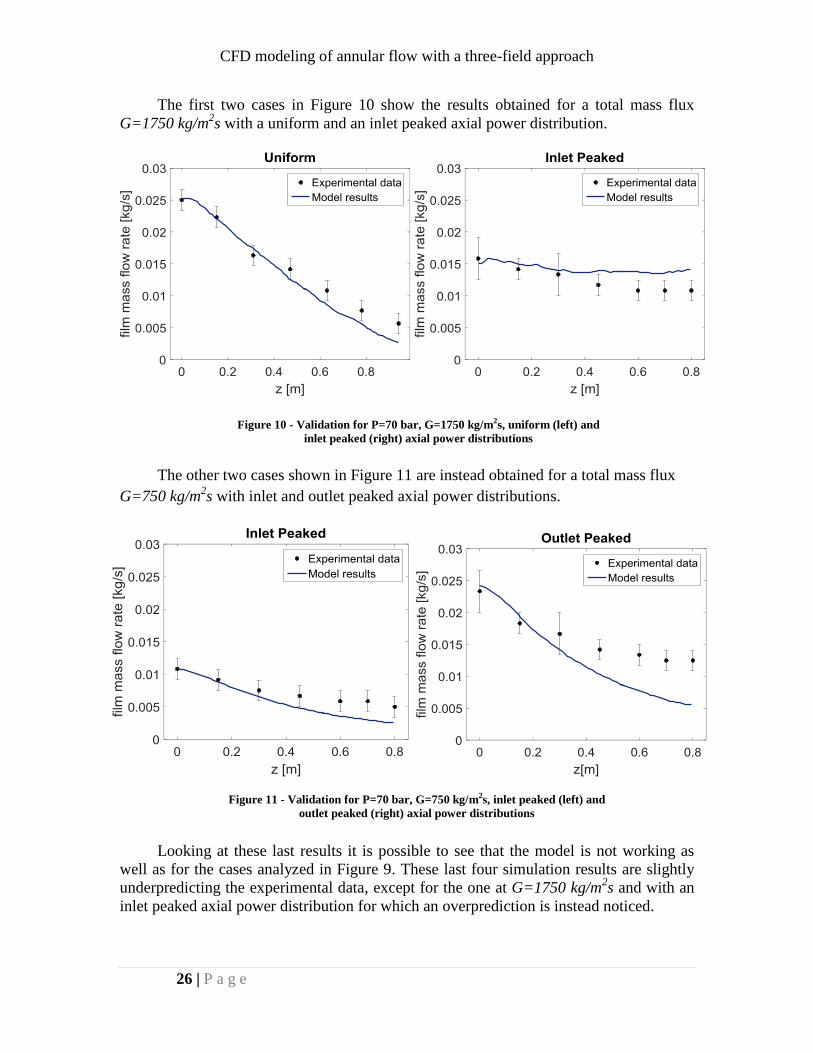
The first two cases in Figure 10 show the results obtained for a total mass flux
G=1750 kg/m2s with a uniform and an inlet peaked axial power distribution.
The other two cases shown in Figure 11 are instead obtained for a total mass flux
G=750 kg/m2s with inlet and outlet peaked axial power distributions.
Looking at these last results it is possible to see that the model is not working as
well as for the cases analyzed in Figure 9. These last four simulation results are slightly
underpredicting the experimental data, except for the one at G=1750 kg/m2s and with an
inlet peaked axial power distribution for which an overprediction is instead noticed.
Figure 10 - Validation for P=70 bar, G=1750 kg/m2s, uniform (left) and
inlet peaked (right) axial power distributions
Figure 11 - Validation for P=70 bar, G=750 kg/m2s, inlet peaked (left) and
outlet peaked (right) axial power distributions

CFD modeling of annular flow with a three-field approach
27 | P a g e
Hence, it can be concluded that the model cannot be used as it is for a wide range of
flow conditions, especially if the total mass flux is changed.
There are different reasons why the model is not responding well when changing
the flow conditions. First of all it could be that the way the inlet conditions are calculated
is not good for every flow condition. In fact the length needed in the development model
could be dependent to flow parameters such as the axial velocity. A slower flow could
require a longer pipe to develop the inlet conditions.
It could also be that some parameters which have not been taken into consideration
during this master thesis influence the model results, for example some constants used in
the Okawa’s entrainment model could also depend on the flow conditions.
However, the main hypothesis is that since the droplet size depends on the flow
conditions, as said in section IV.3, the value chosen of 1.2 mm is only valid for a total
mass flux of 1250 kg/m2s but it should be changed for lower or higher mass fluxes.
To study this hypothesis a simulation of one of the last four cases analyzed
(G=750 kg/m2s and inlet peaked axial power distribution) is done reducing the droplet
diameter from 1.2 mm to 0.3 mm. The results are shown in Figure 12.
As expected from the sensitivity study on droplet diameter, when using a smaller
value of the droplet size, the deposition rate increases leading to a higher film mass flow
rate. The underprediction noticed before is no longer seen and the experimental data are
very well approximated by the model
results.
However, even if the hypothesis
of the droplet diameter seems to be
correct it cannot be stated with 100%
confidence that this is the only reason
leading to the underprediction of the
experimental data for G=750 kg/m2s
or to the overprediction of the
experimental data for G=1750 kg/m2s.
Besides even if it is known from the
studies presented in section IV.3 that
the droplet size is affected by different
flow parameters, there is no evidence
of why a value of 0.3 mm is
appropriate for the particular flow case
analyzed.
Figure 12 - Validation for P=70 bar, G=750 kg/m2s and inlet peaked
axial power distribution with a droplet diameter of 0.3 mm
CFD modeling of annular flow with a three-field approach
28 | P a g e
IV.5. Onset-to-Dryout Simulation
All the validation cases shown above refer to a model which describes a portion of
an already developed annular flow, in which film and droplets inlet conditions are known
and the inlet boundary conditions are calculated in order to meet these conditions.
However, it is of interest to model not only part of the flow but the entire annular flow
starting from the Churn-Annular transition and modeling until dryout happens. The
Churn-Annular transition is also referred to as onset of annular flow and that’s why the
term Onset-to-Dryout simulation is used.
When modeling the whole annular flow starting from the onset, the choice of inlet
boundary conditions becomes complicated. In fact the only thing that can be known with
a certain precision is the steam quality. Therefore it is possible to know the amount of
vapor and liquid in the flow but it is difficult to know which fraction of the liquid is
dispersed as droplets or travel on the wall as liquid film. Besides, the transition zone is a
highly chaotic one and the creation of steam velocity profile and droplet injection file
from outlet condition of another model cannot be done.
On the other hand, when modeling annular flow from the onset to dryout or near
dryout conditions the length of the channel is long and the entrance effects are less
important. In fact for such long distances the flow can develop properly even if the inlet
boundary conditions are far from the real ones. Of course the results in the initial part of
the channel would not be accurate but, since the major interest is on the final part of the
channel, it is a good compromise.
Given that the inlet boundary conditions of droplets and steam velocity are not as
important as for the partial flow modeling, one should still determine the onset
entrainment fraction, which is the fraction of liquid in the form of dispersed droplets.
Some research has been done in this direction, and a few correlations have been
developed with the help of look-up tables. Such tables collect experimental data of
Critical Heat Flux for different flow conditions and can be used to develop correlations
for different parameters. However, even if these correlations have been validated in a
wide range of conditions, the look-up tables are not globally accepted and their results
still have uncertainties [12].
Since it is not easy to find a proper value and given the complexity of the transition
phenomenon it is reasonable to assume that the entrainment fraction in reality is
constantly varying. It is then important to know how much the solution of the model
depends on this parameter.
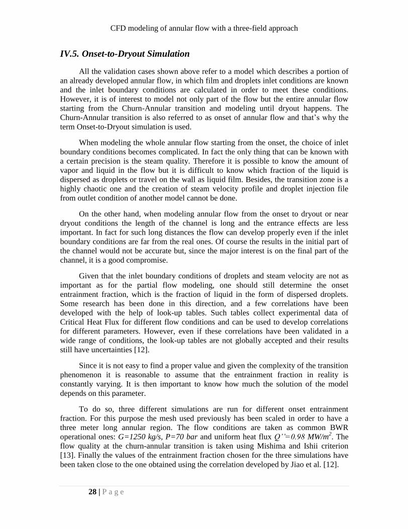
To do so, three different simulations are run for different onset entrainment
fraction. For this purpose the mesh used previously has been scaled in order to have a
three meter long annular region. The flow conditions are taken as common BWR
operational ones: G=1250 kg/s, P=70 bar and uniform heat flux Q’’=0.98 MW/m2. The
flow quality at the churn-annular transition is taken using Mishima and Ishii criterion
[13]. Finally the values of the entrainment fraction chosen for the three simulations have
been taken close to the one obtained using the correlation developed by Jiao et al. [12].
CFD modeling of annular flow with a three-field approach
29 | P a g e
The results of these simulations are shown in Figure 13.
Figure 13 - Sensitivity to onset entrainment fraction E0 in onset-to-dryout simulation
The main outcome of this study is that the results are very sensitive to the onset
entrainment fraction. By changing this value only from 0.51 to 0.60, the dryout position,
which in the figure is the point in which the curves intersect the horizontal axis, is
reduced by around 0.3 meters.
Unfortunately it is not possible to know with the current knowledge on annular
flow, if such sensitivity is reasonable or if it is a flaw of the model.

CFD modeling of annular flow with a three-field approach
30 | P a g e
Chapter V. - Conclusions and Follow-Up
Modeling annular flow with CFD codes turns out to be quite challenging. There are
many boundary conditions and computational settings that have to be analyzed properly
and tuned. Besides there is not a unique way of doing it, many different approaches can
be tried and none of them is with certainty better than the others.
Within this project the main focus is put on the choice of proper inlet boundary
conditions and computational settings in order to obtain valuable results using an
Eulerian-Lagrangian approach. The Lagrangian Particle Tracking brings many
complications since the results given by this method are very dependent on the inlet
conditions. However, the LPT seems to be the best choice to model in 3D the flow of
dispersed droplets within the steam core. This method is simply solving equations of
motion for each parcel tracked so that you do not need to use any correlation to model
deposition. In this way deposition modeling is quite general and applicable to different
geometries and flow conditions.
It is also shown that the main parameters influencing the LPT results are the droplet
inlet velocity, the steam inlet velocity and the droplet diameter.
There is one more inlet flow parameter that could affect the entrance region. This
parameter is the droplet inlet spatial distribution. It has been noticed during the
postprocessing of the different simulations carried out in this project that the droplets
traveling in the steam core develop a certain spatial distribution in which the near-wall
zone is slightly less dense of droplets compared to the inner part of the pipe. At the
current state droplets are injected at the inlet with a uniform spatial distribution. This is
thought to be the best solution at the moment because there are no experimental data to
refer to. However, how this inlet parameter affects the results should be investigated with
a sensitivity study. In fact it could be part of the reason why there is still some difference
between the model results and the experimental data compared in section IV.4.
Regardless of the improvement done in the settings of the inlet boundary conditions
and on the calculation speed of the model that has been noticeably increased, there are
still many aspects that have to be studied and improved in order to have a model that can
be trusted and used in design processes and safety analysis.
The difficulties in doing so are not only related to computational limitation or
difficulties in using the CFD model but also and mainly to the current lack of knowledge
about annular flow itself. This physical process has kept many scientists and researchers
busy for decades but its complexity is so that many things still remain unknown and only
correlations for particular flow conditions and simple geometries have been formulated
so far. Anyway the interest shown on this topic by industries and academic institutions all
over the world and the wider and wider use of CFD codes in many industrial processes let
us hope for a faster and faster development of such models.

CFD modeling of annular flow with a three-field approach
31 | P a g e
Regarding the model developed during this master thesis there are some
recommendations that the author thinks can help for a future development.
First of all in order to be able to use the model for different geometries than pipes
the entrainment modeling need to be changed. Currently the Okawa’s correlation is used
and its validity is restrained to pipe geometries. The best choice would be to use a
correlation which does not depend on the geometry. To do so this correlation should be
developed from only mechanistic consideration in order to give local results at each point
of the liquid film. Using a local correlation that depends only on local flow parameters
like film superficial velocity would also make it possible to use different values of the
diameter of entrained droplets, positively affecting also the deposition modeling. If the
droplet diameter is calculated locally the large sensitivity of the results due to the choice
of a fixed value will also be avoided.
In the recent literature few studies on this topic have been done. Of particular
interest is the work done by Liu and Bai [14]. They propose a correlation based on the
interfacial properties of liquid film waves. Since this correlation is using a force balance
on each wave crest to determine the maximum volume of entrained liquid from each
wave, it could be applied to any geometry. Even though the correlation involves a lot of
parameters which are difficult to get and seems to be quite complicated to apply in the
ANSYS Fluent model via UDFs, it still seems to be the best alternative currently
available.
Another useful article that can help in the development of entrainment modeling is
the research done by Berna et al. in which the authors present and analyze most of the
literature existing on droplets in annular two-phase flow and derive new correlations on
important variables such as amount and size of entrained droplets. Even if Berna et al.
studies refer to pipe geometries some interesting general results depending on local
parameters are achieved [15].
The second main change to do to the model in order to be able to study more cases
is to pass from a structured mesh to an unstructured one. Using structured mesh simplify
the model because the cell faces are either parallel or perpendicular to the main flow
direction. This leads to some simplification in the injection of droplets from a surface via
UDFs or injection file. For example the entrainment mass flow rate is obtained in the
UDF by multiplying the entrainment mass flux obtained from Okawa´s correlation and
the area of the local mesh element face. This can be done because the face of the element
is parallel to the film surface. However, in an unstructured mesh this would not be true
and the value of the area has to be properly calculated in a different way.
This example is not the only case in the UDFs in which the mesh element face area
is used and all of these cases have to be taken into account and changed accordingly
when using an unstructured mesh.
Apart from these main changes which are according to the author the two most
significant ones there is one more change that has to be done especially if dryout and
post-dryout conditions want to be modeled.

CFD modeling of annular flow with a three-field approach
32 | P a g e
This change concerns the evaporation mass source. Since the current model studies
only pre-dryout cases, it is assumed that the whole wall surface of the geometry is wet
with enough film liquid to fully absorb the wall heat flux via evaporation. However,
when simulating general annular flow where dryout can occur, it can happen that part of
the wall is dry and evaporation does not occur leading to a local increase of temperature.
To be able to model this phenomenon the mass source term in the UDF should be re-
written taking into account a condition of sufficient liquid film. Besides the energy
equation should be solved to be able to see the local increase of temperature.

CFD modeling of annular flow with a three-field approach
33 | P a g e
References
[1] Hewitt G.F., Hall-Taylor N.S., 1970. Annular Two-Phase Flow. AERE, Harwell,
England. Pergamon Press.
[2] Henryk Anglart, 2013. Thermal-Hydraulics in Nuclear Systems, Textbook
[3] P. B. Whalley, 1987. Boiling, Condensation and Gas-Liquid Flow. Oxford Science
publications. Clarendon Press, Oxford
[4] Cousins L.B., Denton W.H., and Hewitt G.F., 1965. Liquid mass transfer in annular
two-phase flow. Two-phase flow symposium, Exeter, UK
[5] ANSYS, Inc. 2017. ANSYS Fluent Theory Guide 18.0
[6] Secondi F., Adamsson C., Le Corre J.-M., 2009. An assessment of Entrainment
Correlations for the Dryout Prediction in BWR Fuel Bundles. NURETH-13, Kanazawa
City, Japan
[7] Okawa T., Kotani A., Kataoka I., Naito M., 2003. Prediction of Critical Heat Flux in
Annular Flow Using a Film Flow Model. Journal of Nuclear Science and Technology,
Vol. 40, No.6
[8] Camacho M., 2016. CFD modeling of annular flow to predict behavior of the liquid
film. SES_16-094_rev_0
[9] ANSYS, Inc. 2017. ANSYS Fluent User’s Guide 18.0
[10] Adamsson C., Anglart H., 2006. Film flow measurements for high-pressure diabatic
annular flow in tubes with various axial power distributions. Nuclear Engineering and
Design 236 (2006) 2485-2493
[11] Le Corre J.-M., Bergmann U.C., Hallen A., Tejne H., Waldemarsson F., Morenius
B., Baghai R., 2015. Detailed measurements of local parameters in annular two-phase
flow in fuel bundle under BWR operating conditions. NURETH-16, Chicago, US
[12] Jiao B., Yang D., Gan Z., 2017. An empirical correlation for the entrainment
fraction at the onset of annular flow based on 2006 CHF look-up table. Nuclear
engineering and Design 317 (2017) 69-80
[13] Mishima C., Ishii M., 1983. Flow regime transition criteria for upward two-phase
flow in vertical tubes. International Journal of Heat and Mass Transfer. Vol.27, No. 5, pp.
723-737, 1984
[14] Liu L., Bai B., 2017. Generalization of droplet entrainment rate correlation for
annular flow considering disturbance wave properties. Chemical Engineering Science
164 (2017) 279-291

CFD modeling of annular flow with a three-field approach
34 | P a g e
[15] Berna C., Escrivá A., Munoz-Cobo J.L., Herranz L.E., 2014. Review of droplet
entrainment in annular flow: Characterization of the entrained droplets. Progress in
Nuclear Energy 79 (2015) 64-86

CFD modeling of annular flow with a three-field approach
35 | P a g e
Appendices
Appendix A – User Defined Functions
Below is an example of the User Defined Functions used during the simulations. To
simulate different flow conditions a few parameters have to be changed and sometimes
also entire part of the UDF has to be changed or deleted. The script presented in this
appendix contains all the different UDFs used throughout the whole master thesis project.
Therefore, pay attention when using them to be sure to make the right modification to fit
the flow conditions you are simulating.
#include "udf.h"
#include "sg_film.h"
real hvap = 1504900;
real heat_flux_mean = 983443;
real n = 0.111;
real ke = 0.000479;
real rhovap = 36.525;
real rholiq = 739.72;
real dh = 0.014;
real r = 0.007;
real muliq = 0.000091249;
real Ref_crit = 320;
real sigma = 0.017633;
real p_diam = 0.0012;
DEFINE_PROFILE(film_mass_source,tf,i)
{
real film_thickness, film_vel, vap_vel, Jf, Jg, fi, Ref, area_face,
area[ND_ND], pos[ND_ND], r1, x_inj, y_inj, z_inj, evap_mass_source,
evap_mom_source, ent_mass_source, distrib;
face_t f;
cell_t c;
Thread *tc;
begin_f_loop(f,tf)
{
film_thickness = F_EFILM_HEIGHT(f,tf);
film_vel = F_EFILM_W(f,tf);
c = F_C0(f,tf);
tc = THREAD_T0(tf);
F_CENTROID(pos,f,tf);
vap_vel = 0.6543*pos[2]*pos[2]*pos[2]-7.706*pos[2]*pos[2]+
32.44*pos[2]-28.95;
Jf = 4*film_vel*film_thickness/dh;
Jg = vap_vel;
fi = 0.005*(1+300*(film_thickness/dh));
Ref = (rholiq*Jf*dh)/muliq;
if (Ref>Ref_crit)

CFD modeling of annular flow with a three-field approach
36 | P a g e
ent_mass_source =
((ke*rholiq*fi*rhovap*Jg*Jg*film_thickness)/sigma)*pow
(rholiq/rhovap,n);
else
ent_mass_source = 0.0;
distrib=-0.041572*pow(pos[2],6)+0.43222*pow(pos[2],5)-1.5111
*pow(pos[2],4)+1.7822*pow(pos[2],3)-0.036178*pow(pos[2],2)+
0.094166*pos[2]+0.4022;
evap_mass_source = distrib*heat_flux_mean/hvap;
evap_mom_source = evap_mass_source*film_vel;
F_AREA(area,f,tf);
area_face = NV_MAG(area);
r1 = r-5*film_thickness;
x_inj = r1*(pos[0]/r);
y_inj = r1*(pos[1]/r);
z_inj = pos[2];
C_UDMI(c,tc,0) = evap_mass_source;
C_UDMI(c,tc,1) = evap_mass_source*area_face;
C_UDMI(c,tc,2) = evap_mom_source;
C_UDMI(c,tc,3) = evap_mom_source*area_face;
C_UDMI(c,tc,4) = ent_mass_source;
C_UDMI(c,tc,5) = ent_mass_source*area_face;
C_UDMI(c,tc,6) = x_inj;
C_UDMI(c,tc,7) = y_inj;
C_UDMI(c,tc,8) = z_inj;
C_UDMI(c,tc,12) = F_EFILM_DPM_MASS_SRC(f,tf)/area_face;
C_UDMI(c,tc,13) = F_EFILM_WS(f,tf);
F_PROFILE(f,tf,i) = -(ent_mass_source+evap_mass_source);
}end_f_loop(f,tf)
}
DEFINE_DPM_INJECTION_INIT(entrainment_inj,I)
{
Particle *p;
cell_t c;
Thread *tc;
loop(p,I->p_init)
{
c = P_CELL(p);
tc = P_CELL_THREAD(p);
P_POS(p)[0]=C_UDMI(c,tc,6);
P_POS(p)[1]=C_UDMI(c,tc,7);
P_POS(p)[2]=C_UDMI(c,tc,8);

CFD modeling of annular flow with a three-field approach
37 | P a g e
P_FLOW_RATE(p)= C_UDMI(c,tc,5);
P_DIAM(p)=p_diam;
P_VEL(p)[0]=C_U(c,tc);
P_VEL(p)[1]=C_V(c,tc);
P_VEL(p)[2]=C_W(c,tc);
C_UDMI(c,tc,9)=C_U(c,tc);
C_UDMI(c,tc,10)=C_V(c,tc);
C_UDMI(c,tc,11)=C_W(c,tc);
}
}
DEFINE_DPM_INJECTION_INIT(inlet_inj,I)
{
Particle *p;
cell_t c;
Thread *tc;
face_t f;
Thread *tf;
int n;
real x[ND_ND],area_face,area[ND_ND];
loop(p,I->p_init)
{
c = P_CELL(p);
tc = P_CELL_THREAD(p);
real area_min=1;
c_face_loop(c,tc,n)
{
f = C_FACE(c,tc,n);
tf = C_FACE_THREAD(c,tc,n);
F_AREA(area,f,tf);
area_face = NV_MAG(area);
if(area_face<=area_min)
area_min=area_face;
}
C_CENTROID(x,c,tc);
P_POS(p)[0]=x[0];
P_POS(p)[1]=x[1];
P_POS(p)[2]=x[2];
P_FLOW_RATE(p)=581.1*area_min;
P_DIAM(p)=p_diam;
P_VEL(p)[0]=0;
P_VEL(p)[1]=0;
P_VEL(p)[2]=C_W(c,tc);
}
}
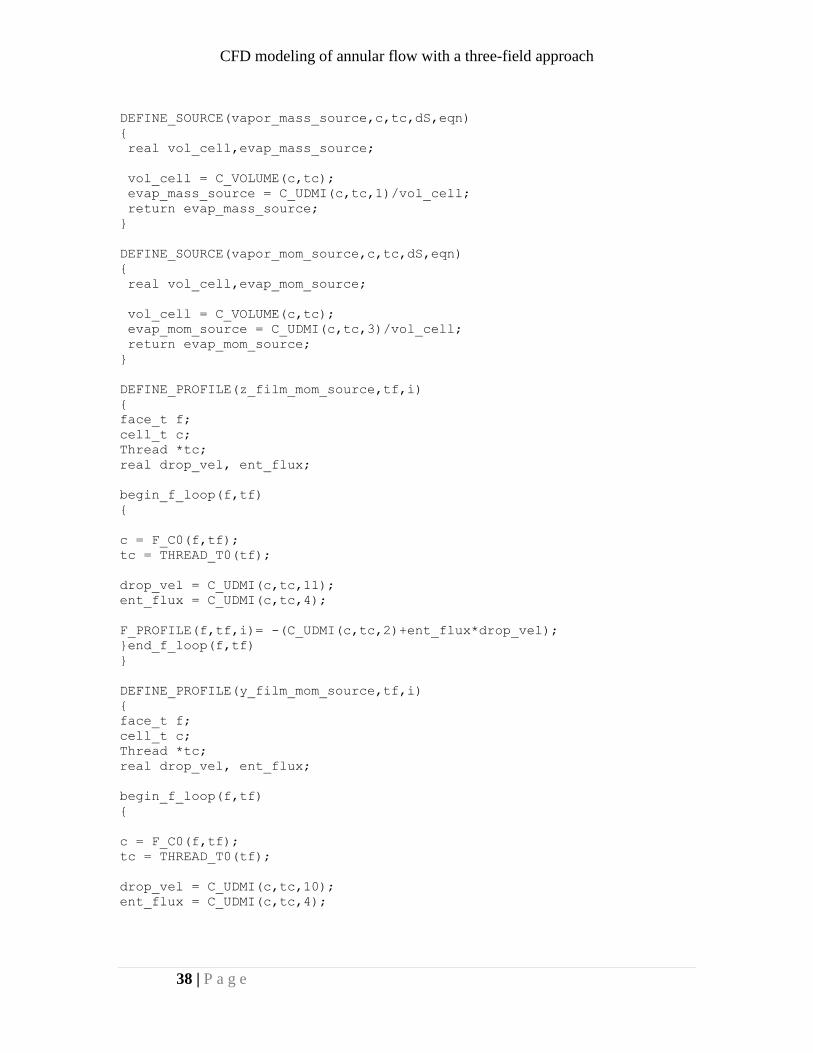
CFD modeling of annular flow with a three-field approach
38 | P a g e
DEFINE_SOURCE(vapor_mass_source,c,tc,dS,eqn)
{
real vol_cell,evap_mass_source;
vol_cell = C_VOLUME(c,tc);
evap_mass_source = C_UDMI(c,tc,1)/vol_cell;
return evap_mass_source;
}
DEFINE_SOURCE(vapor_mom_source,c,tc,dS,eqn)
{
real vol_cell,evap_mom_source;
vol_cell = C_VOLUME(c,tc);
evap_mom_source = C_UDMI(c,tc,3)/vol_cell;
return evap_mom_source;
}
DEFINE_PROFILE(z_film_mom_source,tf,i)
{
face_t f;
cell_t c;
Thread *tc;
real drop_vel, ent_flux;
begin_f_loop(f,tf)
{
c = F_C0(f,tf);
tc = THREAD_T0(tf);
drop_vel = C_UDMI(c,tc,11);
ent_flux = C_UDMI(c,tc,4);
F_PROFILE(f,tf,i)= -(C_UDMI(c,tc,2)+ent_flux*drop_vel);
}end_f_loop(f,tf)
}
DEFINE_PROFILE(y_film_mom_source,tf,i)
{
face_t f;
cell_t c;
Thread *tc;
real drop_vel, ent_flux;
begin_f_loop(f,tf)
{
c = F_C0(f,tf);
tc = THREAD_T0(tf);
drop_vel = C_UDMI(c,tc,10);
ent_flux = C_UDMI(c,tc,4);
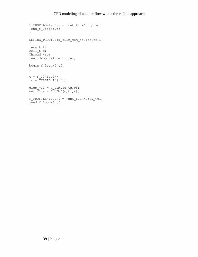
CFD modeling of annular flow with a three-field approach
39 | P a g e
F_PROFILE(f,tf,i)= -ent_flux*drop_vel;
}end_f_loop(f,tf)
}
DEFINE_PROFILE(x_film_mom_source,tf,i)
{
face_t f;
cell_t c;
Thread *tc;
real drop_vel, ent_flux;
begin_f_loop(f,tf)
{
c = F_C0(f,tf);
tc = THREAD_T0(tf);
drop_vel = C_UDMI(c,tc,9);
ent_flux = C_UDMI(c,tc,4);
F_PROFILE(f,tf,i)= -ent_flux*drop_vel;
}end_f_loop(f,tf)
}

CFD modeling of annular flow with a three-field approach
40 | P a g e
Appendix B – Injection File
The injection file is a way of defining the injection in the DPM. It is used to inject
droplets specifying for each injected parcel its spatial coordinate, velocity components,
diameter, temperature and mass flow rate. These files are text file in which each line
corresponds to an injection. Here, it is shown the formatting of one line in an injection
file.
(( x y z x-vel y-vel z-vel diameter temperature mass-flow-rate ))
In the model these values are extracted from the solution of the inlet development model.
Using File Extract Solution Data it is possible to extract and save
these values in a ASCII format. To convert this file into an injection file, a MATLAB and
a C language script are used. In MATLAB it is possible to import the ASCII file and save
it in a matrix where the values for the z coordinate and mass-flow-rate can be adjusted to
meet the value needed as inlet condition for the injection of the main model. Once this is
done, the matrix can be saved or simply copy pasted in a .txt file. The C script then reads
the .txt file and creates a new .txt file called “nuovo.txt” with the right formatting of the
lines (double brackets at the beginning and end of each line, space divided values).
Finally the decimal sign has to be changed from coma to dot and the extension of the file
has to be changed from .txt to .inj. This can be done simply renaming the file and
changing the extension in the name.
To run the C script via the terminal go to the directory which contain the script and the
injection.txt file and run the following command:
./nameofthescript nameotheinjectionfile.txt
The name of the script and the file commonly used in the project are respectively
“injectionCprogram” and “inj.txt” . The final injection file is then called “injection0.inj”

CFD modeling of annular flow with a three-field approach
41 | P a g e
Appendix C – 1D Code
The following MATLAB script is used to model in 1D the same flow modeled with
ANSYS Fluent in order to have something else to compare the results with other than
experimental data. This particular script refers to the following flow conditions: P=70
bar, G=1250 kg/m2s and uniform power distribution.
R=0.007;
A=pi*R*R;
dropd=0.0012;
muliq=0.000091249;
mugas=0.000018960;
rho=36.525;
rhol=739.72;
m1drop=4/3*pi*(dropd/2)^3*rhol;
D=0.014;
H=1504900;
q_sec=983443;
sigma=0.017633;
en=0.111;
ke=0.000479;
g=9.81;
vi=12.0352;
Z=1.06;
G=1250;
M=G*A;
h=0.001;
N=round(Z/h);
mvap=zeros(1,N);
mdrop=zeros(1,N);
mfilm=zeros(1,N);
filmthi=zeros(1,N);
filmvel=zeros(1,N);
ment=zeros(1,N);
mdep=zeros(1,N);
steamvel=zeros(1,N);
mdrop(1)= 0.0989;
mfilm(1)=0.0258;
mvap(1)=M-mfilm(1)-mdrop(1);
Mtot(1)=M;
steamvel(1)=vi;
Ment=0;
Mdep=0;
z=(h:h:Z);
film_vel1 = vi;
film_thickness1=R-(R*R-mfilm(1)/pi/rhol/film_vel1)^0.5;
Jf = 4*film_vel1*film_thickness1/D;
Jg = vi;
Ref = (rhol*Jf*D)/muliq;
fi1 = 0.005*(1+300*(film_thickness1/D));
film_thickness2 = 0.25*sqrt(max(16/Ref,0.005)*rhol/(fi1*rho))*Jf*D/Jg;
fi2 = 0.005*(1+300*(film_thickness2/D));
delta=abs(fi2-fi1);

CFD modeling of annular flow with a three-field approach
42 | P a g e
while delta>0.001*fi1
film_vel2 = film_vel1*(R*R-(R-film_thickness1)*(R-
film_thickness1))/(R*R-(R-film_thickness2)*(R-
film_thickness2));
Jf = 4*film_vel2*film_thickness2/D;
fi1 = 0.005*(1+300*(film_thickness2/D));
film_thickness1 = film_thickness2;
film_vel1 = film_vel2;
film_thickness2 =
0.25*sqrt(max(16/Ref,0.005)*rhol/(fi1*rho))*Jf*D/Jg;
fi2 = 0.005*(1+300*(film_thickness2/D));
delta=abs(fi2-fi1);
end
filmthi(1)=film_thickness1;
filmvel(1)=film_vel1;
for i=2:N
mvap(i)=mvap(i-1)+(q_sec/H)*h*2*pi*R;
steamvel(i)=mvap(i)/rho/A;
Jf = 4*filmvel(i-1)*filmthi(i-1)/D;
Jg = steamvel(i-1);
Ref = (rhol*Jf*D)/muliq;
fi = 0.005*(1+300*(filmthi(i-1)/D));
ment(i-1)=ke*rhol*fi*rho*Jg*Jg*filmthi(i-1)*((rhol/rho)^en)/sigma;
vd=steamvel(i-1)-0.23;
C=mdrop(i-1)/(vd*A);
mdep(i-1)=C*0.0632*((C/rho)^(-0.5))*((rho*D/sigma)^(-0.5));
Ment=Ment+ment(i-1)*h*2*pi*R;
Mdep=Mdep+mdep(i-1)*h*2*pi*R;
mfilm(i)=mfilm(1)-Ment+Mdep-mvap(i)+mvap(1);
filmthi(i) = 0.25*sqrt(max(16/Ref,0.005)*rhol/(fi*rho))*Jf*D/Jg;
filmvel(i) = mfilm(i)/(rhol*pi*(R^2-(R-filmthi(i))^2));
mdrop(i)=mdrop(1)+Ment-Mdep;
Mtot(i)=mdrop(i)+mfilm(i)+mvap(i);
end