cfa: a practical prediction system for video qoe …junchenj/cfa.pdf · usenix association 13th...

USENIX Association 13th USENIX Symposium on Networked Systems Design and Implementation (NSDI ’16) 137

CFA: A Practical Prediction System for Video QoE Optimization

Junchen Jiang†, Vyas Sekar†, Henry Milner⋆, Davis Shepherd+, Ion Stoica⋆+◦, Hui Zhang†+

†CMU, ⋆UC Berkeley, +Conviva, ◦Databricks

AbstractMany prior efforts have suggested that Internet videoQuality of Experience (QoE) could be dramatically im-proved by using data-driven prediction of video qualityfor different choices (e.g., CDN or bitrate) to make opti-mal decisions. However, building such a prediction sys-tem is challenging on two fronts. First, the relationshipsbetween video quality and observed session features canbe quite complex. Second, video quality changes dy-namically. Thus, we need a prediction model that is(a) expressive enough to capture these complex relation-ships and (b) capable of updating quality predictions innear real-time. Unfortunately, several seemingly natu-ral solutions (e.g., simple machine learning approachesand simple network models) fail on one or more fronts.Thus, the potential benefits promised by these prior ef-forts remain unrealized. We address these challenges andpresent the design and implementation of Critical Fea-ture Analytics (CFA). The design of CFA is driven bydomain-specific insights that video quality is typicallydetermined by a small subset of critical features whosecriticality persists over several tens of minutes. This en-ables a scalable and accurate workflow where we auto-matically learn critical features for different sessions oncoarse-grained timescales, while updating quality pre-dictions in near real-time. Using a combination of areal-world pilot deployment and trace-driven analysis,we demonstrate that CFA leads to significant improve-ments in video quality; e.g., 32% less buffering time and12% higher bitrate than a random decision maker.

1 IntroductionDelivering high quality of experience (QoE) is crucialto the success of today’s subscription and advertisement-based business models for Internet video. As prior work(e.g., [33, 11]) has shown, achieving good QoE is chal-lenging because of significant spatial and temporal vari-ation in CDNs’ performance, client-side network condi-tions, and user request patterns.

At the same time, these observations also suggest thereis a substantial room for improving QoE by dynamicallyselecting the optimal CDN and bitrate based on a real-time global view of network conditions. Building on this

History of quality measurements Decision Maker

Video Streaming Ecosystem

asurem Decision Makments surem

Global Optimization System

Global view of video quality

Quality prediction of potential decision

Prediction System

f lit

Figure 1: Overview of a global optimization system andthe crucial role of a prediction system.insight, prior work makes the case for a quality optimiza-tion system (Figure 1) that uses a prediction oracle tosuggest the best parameter settings (e.g., bitrate, CDN)to optimize quality (e.g., [33, 11, 35, 32, 20]). Seen in abroader context, this predictive approach can be appliedbeyond Internet video (e.g., [10, 40, 15, 16, 43]).

However, these prior efforts fall short of providinga concrete instantiation of such a prediction system.Specifically, we observe that designing such a predictionsystem is challenging on two key fronts (§2):

• Capturing complex factors that affect quality: Forinstance, an outage may affect only clients of a spe-cific ISP in a specific city when they use a specificCDN. To accurately predict the quality of their ses-sions, one must consider the combination of all threefactors. In addition, the factors that affect video qual-ity vary across different sessions; e.g., wireless hostsmay be bottlenecked at the last connection, whileother clients may experience loading failures due tounavailability of specific content on some CDNs.

• Need for fresh updates: Video quality changesrapidly, on a timescale of several minutes. Ideally, wemust make predictions based on recent quality mea-surements. This is particularly challenging given thevolume of measurements (e.g., YouTube had 231 mil-lion video sessions and up to 500 thousand concurrentviewers during the Olympics [7]), compounded withthe need for expressive and potentially complex pre-diction models.

Unfortunately, many existing solutions fail on one or

1

Appeared in Proceedings of the 13th USENIX Symposium on Networked Systems Design and Implementation (NSDI ’16)

138 13th USENIX Symposium on Networked Systems Design and Implementation (NSDI ’16) USENIX Association

both counts. For instance, solutions that use less complexmodels (e.g., linear regression, Naive Bayes, or simplemodels based on last-mile connection) are not expressiveenough to capture high dimensional and diverse relation-ships between video quality and session features. Morecomplex algorithms (e.g., SVM [42]) can take severalhours to train a prediction model and will be inaccuratebecause predictions will rely on stale data.

In this work, we address these challenges and presentthe design and implementation of a quality predictionsystem called Critical Feature Analytics (CFA). CFA isbuilt on three key domain-specific insights:

1. Video sessions with same feature values have similarquality. This naturally leads to an expressive model,wherein the video quality of a given session can be ac-curately predicted based on the quality of sessions thatmatch values on all features (same ASN, CDN, player,geographical region, video content, etc). However, ifapplied naively, this model can suffer from the curseof dimensionality — as the number of combinations offeature values grows, it becomes hard to find enoughmatching sessions to make reliable predictions.

2. Each video session has a subset of critical featuresthat ultimately determines its video quality. Given thisinsight, we can make more reliable predictions basedon similar sessions that only need to match on criti-cal features. For example, in a real event that we ob-served, congestion of a Level3 CDN led to relativelyhigh loading failure rate for Comcast users in Balti-more. We can accurately predict the quality of the af-fected sessions using sessions associated with the spe-cific CDN, region and ISP, ignoring other non-criticalfeatures (e.g., player, video content). Thus, this tack-les the curse of dimensionality, while still retainingsufficient expressiveness for accurate prediction (§3).

3. Critical features tend to be persistent. Two remain-ing concerns are: (a) Can we identify critical featuresand (b) How expensive is it to do so? The insighton persistence implies that critical features are learn-able from recent history and can be cached and reusedfor fast updates (§4). This insight is derived from re-cent measurement studies [25, 20] (e.g., the factorsthat lead to poor video quality persist for hours, andsometimes, even days).

Taken together, these insights enable us to engineera scalable and accurate video quality prediction system.Specifically, on a coarse timescale of tens of minutes,CFA learns the critical features, and on a fine timescaleof minutes, CFA updates quality prediction using recentquality measurements. CFA makes predictions and deci-sions as new clients arrive.

We implemented a prototype of CFA and integratedit in a video optimization platform that manages many

premium video providers. We ran a pilot study on onecontent provider that has 150,000 sessions each day. Ourreal-world experiments show that the bitrates and CDNsselected by CFA lead to 32% less buffering time and 12%higher bitrate than a baseline random decision maker.Using real trace-driven evaluation, we also show thatCFA outperforms many other simple ML prediction al-gorithms by up to 30% in prediction accuracy and 5-17%in various video quality metrics.Contributions and Roadmap:• Identifying key challenges in building an accurate pre-

diction system for video quality (§2).• Design and implementation of CFA, built on domain-

specific insights to address the challenges (§3-5).• Real-world and trace-driven evaluation that demon-

strates substantial quality improvement by CFA (§6).• Using critical features learned by CFA to make inter-

esting observations about video quality (§7).

2 Background and ChallengesThis section begins with some background on videoquality prediction (§2.1). Then, we articulate two keychallenges faced by any video quality prediction system:(1) The factors affecting video quality are complex, sowe need expressive models (§2.2); (2) Quality changesrapidly, so models must be updated in near real-time byrecent quality measurements (§2.3). We also argue whyexisting solutions do not address these challenges.

2.1 BackgroundMost video service providers today allow a video client(player) to switch CDN and bitrate among a set of avail-able choices [33, 20, 32]. These switches have little over-head and can be performed at the beginning of and dur-ing a video playback [8]. Our goal then is to choose thebest CDN and bitrate for a client by accurately predict-ing the video quality of each hypothetical choice of CDNand bitrate. In theory, if we can accurately predict thequality of each potential decision, then we can identifythe optimal decision.

To this end, we envision a prediction system that uses aglobal view of quality measurements to make predictionsfor a specific video session. It learns a prediction func-tion for each quality metric Pred : 2S × S "→ R, whichtakes as input a given set of historical sessions S ∈ 2Swhose quality is already measured, and a new sessions ∈ S, and outputs a quality prediction p ∈ R for s.

Each quality measurement summarizes the quality of avideo session for some duration of time (in our case, oneminute). It is associated with values of four quality met-rics [18] and a set of features2 (summarized in Table 1).

1For one session, VSF is zero if it starts successfully, one otherwise.2By feature, we refer to the type of attribute (e.g., CDN), rather than

value of these attributes (e.g., CDN = Akamai)

2


Metrics DescriptionBufRatio Fraction of time a session spends in buffering

(smooth playback is interrupted by buffering).AvgBitrate Time-weighted average of bitrates in a session.JoinTime Delay for the video to start playing from the time

the user clicks “play”.Video start fail-ure (VSF)

Fraction of sessions that fail to start playing(e.g., unavailable content or overloaded server)1.

Features DescriptionASN Autonomous System to which client IP belongs.City City where the client is located.ConnectionType Type of access network; e.g., mobile/fixed wire-

less, DSL, fiber-to-home [3].Player e.g., Flash, iOS, Silverlight, HTML5.Site Content provider of requested video contents.LiveOrVoD Binary indicator of live vs. VoD content.ContentName Name of the requested video object.CDN CDN a session started with.Bitrate Bitrate value the session started at.

Table 1: Quality metrics and session features associ-ated with each session. CDN and Bitrate refer to initialCDN/bitrate values as we focus on initial selections.In general, the set of features depends on the degree ofinstrumentation and what information is visible to a spe-cific provider. For instance, a CDN may know the loca-tion of servers, whereas a third-party optimizer [1] mayonly have information at the CDN granularity. Our fo-cus is not to determine the best set of features that shouldbe recorded for each session, but rather engineer a pre-diction system that can take an arbitrary set of featuresas inputs and extract the relationships between these fea-tures and video quality. In practice, the above set of fea-tures can already provide accurate predictions that helpimprove quality.

Our dataset consists of 6.6 million quality measure-ments collected from 2 million clients using 3 large pub-lic CDNs distributed across 168 countries and 152 ISPs.

2.2 Challenge 1: Expressive modelsWe show real examples of the complex factors that im-pact video quality, and the limitations in capturing theserelationships.High-dimensional relationship between video qualityand session features. Video quality could be impactedby combinations of multiple components in the network.Such high-dimensional effects make it harder to learn therelationships between video quality and features, in con-trast to simpler settings where features affect quality in-dependently (e.g., assumed by Naive Bayes).

In a real-world incident, video sessions of Comcastusers in Baltimore who watched videos from Level3CDN experienced high failure rate (VSF) due to con-gested edge servers, shown by the blue line in Figure 2.The figure also shows the VSF of sessions sharing thesame values on one or two features with the affected ses-sions; e.g., all Comcast sessions across different citiesand CDNs. In the figure, the high VSF of the affectedsessions cannot be clearly identified if we look at the ses-

0 0.2 0.4 0.6 0.8

0 5 10 15 20 25

VS

F

Time (hour)

3-Feature Best 2-Feature Best 1-Feature Global

Figure 2: The high VSF is only evident when three fac-tors (CDN, ISP and geo-location) are combined.sions that match on only one or two features. Only whenthree features of CDN (“Level3”), ASN (“Comcast”) andCity (“Baltimore”) are specified (i.e., blue line), can wedetect the high VSF and predict the quality of affectedsessions accurately.

In practice, we find that such high-dimensional effectsare the common case, rather than an anomalous cornercase. For instance, more than 65% of distinct CDN-ISP-City values have VSF that is at least 50% higher or lowerthan the VSF of sessions matching only one or two fea-tures (not shown). In other words, their quality is af-fected by a combined effect of at least three features.Limitation of existing solutions: It might be tempting todevelop simple predictors; e.g., based on the last-hopconnection by using average quality of history sessionswith the same ConnectionType value. However, they donot take into account the combined impact of features onvideo quality. Conventional machine learning techniqueslike Naive Bayes also suffer from the same limitation.In Figures 3(a) and 3(b), we plot the actual JoinTimeand the prediction made by the last-hop predictor andNaive Bayes (from Weka [6]) for 300 randomly sampledsessions. The figures also show the mean relative error( |predicted−actual|

actual ). For each session, the prediction algo-rithms train models using historical sessions within a 10-minute interval prior to the session under prediction. Itshows that the prediction error of both solutions is signif-icant and two-sided (i.e., not fixable by normalization).Highly diverse structures of factors. The factors thataffect video quality vary across different sessions. Thismeans the prediction algorithm should be expressiveenough to predict quality for different sessions using dif-ferent prediction models. For instance, the fact that manyfiber-to-the-home (e.g., FiOS) users have high bitratesand people on cellular connections have lower bitratesis largely due to the speed of their last-mile connection.In contrast, some video clients may experience videoloading failures due to unavailability of specific contenton some CDNs. A recent measurement study [25] hasshown that many heterogeneous factors are correlatedwith video quality issues. In §7, we show that 15% ofvideo sessions are impacted by more than 30 differentcombinations of features and give real examples of dif-ferent factors that affect quality.Limitation of existing solutions: To see why existing so-lutions are not sufficient, let us consider the k-nearest

3


0

10

20

30

0 10 20 30Pre

dic

ted J

oin

Tim

e (

sec)

Actual JoinTime (sec)

(a) Last hop (0.76)

0

10

20

30

0 10 20 30Pre

dic

ted J

oin

Tim

e (

sec)


(b) Naive Bayes (0.61)

0

10

20

30

0 10 20 30Pre

dic

ted J

oin

Tim

e (

sec)


(c) k-NN (0.63)

Figure 3: Prediction error of some existing solutions issubstantial (mean of relative error in parentheses).neighbor (k-NN) algorithm. It does not handle diverserelationships between quality and features, because thesimilarity between sessions is based on the same func-tion of features independent of the specific session un-der prediction. In Figure 3(c), we plot the actual valuesof JoinTime and the prediction made by k-NN with thesame setup as Figure 3(a)(b). Similar to Naive Bayesand the last-hop predictor, k-NN has substantial predic-tion error.

2.3 Challenge 2: Fresh updatesVideo quality has significant temporal variability. In Fig-ure 4(a), for each quality metric and combination of spe-cific CDN, city and ASN, we compute the mean qual-ity of sessions in each 10-minute interval, and then plotthe CDF of the relative standard deviation ( stddev

mean ) of thequality across different intervals. In all four quality met-rics of interest, we see significant temporal variability;e.g., for 60% of CDN-city-ASN combinations, the rela-tive standard deviation of JoinTime across different 10-minute intervals is more than 30%. Such quality variabil-ity has also been confirmed in other studies (e.g., [33]).

The implication of such temporal variability is that theprediction system must update models in near real-time.In Figure 4(b), we use the same setup as Figure 3, exceptthat the time window used to train prediction models isseveral minutes prior to the session under prediction. Thefigure shows the impact of such staleness on the predic-tion error for JoinTime. For both algorithms, predictionerror increases dramatically if the staleness exceeds 10minutes. As we will see later, this negative impact ofstaleness on accuracy is not specific to these predictionalgorithms (§6.3).Limitation of existing solutions: The requirement to usethe most recent measurements makes it infeasible to usecomputationally expensive models. For instance, it takesat least one hour to train an SVM-based prediction modelfrom 15K quality measurements in a 10-minute intervalfor one video site, so the quality predictions will be basedon information from more than one hour ago.

3 Intuition behind CFAThis section presents the domain-specific insights we useto help address the expressiveness challenge (§2.2). Thefirst insight is that sessions matching on all features havesimilar video quality. However, this approach suffers

0

0.2

0.4

0.6

0.8

1

0.1 1 10

CD

F

Relative stddev

BufRatioAvgBitrate

JoinTimeVSF

(a) Temporal variability

0

5

10

15

20

1 2 4 8 16

% in

cre

ase

in a

vg

pre

dic

tion

err

or

Staleness (min)

Naive Bayesk-NN

(b) Impact of staleness on accuracy

Figure 4: Due to significant temporal variability ofvideo quality (left), prediction error increases dramati-cally with stale data (right).

Input: Session under prediction s, Previous sessions SOutput: Predicted quality p/* S′:identical sessions matching on all

features with s in recent history(∆) */1 S′ ← SimilarSessionSet(s,S,AllFeatures,∆);/* Summarize the quality (e.g.,median) of

the identical sessions in S′. */2 p ← Est(S′);3 return p;

Algorithm 1: Baseline prediction that finds ses-sions matching on all features and uses their ob-served quality as the basis for prediction.

from the curse of dimensionality. Fortunately, we canleverage a second insight that each video session has asubset of critical features that ultimately determine itsvideo quality. We conclude this section by highlightingtwo outstanding issues in translating these insights into apractical prediction system.

3.1 Baseline prediction algorithmOur first insight is that sessions that have identical fea-ture values will naturally have similar (if not identical)quality. For instance, we expect that all Verizon FiOSusers viewing a specific HBO video using Level3 CDNin Pittsburgh at Fri 9 am should have similar quality(modulo very user-specific effects such as local Wi-Fiinterference inside the home). We can summarize theintuition as follows:

Insight 1: At a given time, video sessions having samevalue on every feature have similar video quality.

Inspired by Insight 1, we can consider a baseline al-gorithm (Algorithm 1). We predict a session’s qualitybased on “identical sessions”, i.e., those from recent his-tory that match values on all features with the session un-der prediction. Ideally, given infinite data, this algorithmis accurate, because it can capture all possible combina-tions of factors affecting video quality.

However, this algorithm is unreliable as it suffersfrom the classical curse of dimensionality [39]. Specif-ically, given the number of combinations of feature val-ues (ASN, device, content providers, CDN, just to namea few), it is hard to find enough identical sessions needed

4


to make a robust prediction. In our dataset, more than78% of sessions have no identical session (i.e., matchingon all features) within the last 5 minutes.

3.2 Critical featuresIn practice, we expect that some features are more likelyto “explain” the observed quality of a specific video ses-sion than others. For instance, if a specific peering pointbetween Comcast and Netflix in New York is congested,then we expect most of these users will suffer poor qual-ity, regardless of the speed of their local connection.

Insight 2: Each video session has a subset of criticalfeatures that ultimately determines its video quality.

We already saw some real examples in §2.2: in theexample of high dimensionality, the critical featuresof the sessions affected by the congested Level3 edgeservers are {ASN,CDN,City}; in the examples of di-versity, the critical features are {ConnectionType} and{CDN,ContentName}. Table 2 gives more real exam-ples of critical features that we have observed in opera-tional settings and confirmed with domain experts.

Quality issue Set of critical featuresIssue on one player of Vevo {Player,Site}ESPN flipping between CDNs {CDN,Site,ContentName}Bad Level3 servers for Com-cast users in Maryland

{CDN,City,ASN}

Table 2: Real-world examples of critical features con-firmed by analysts at a large video optimization vendor.

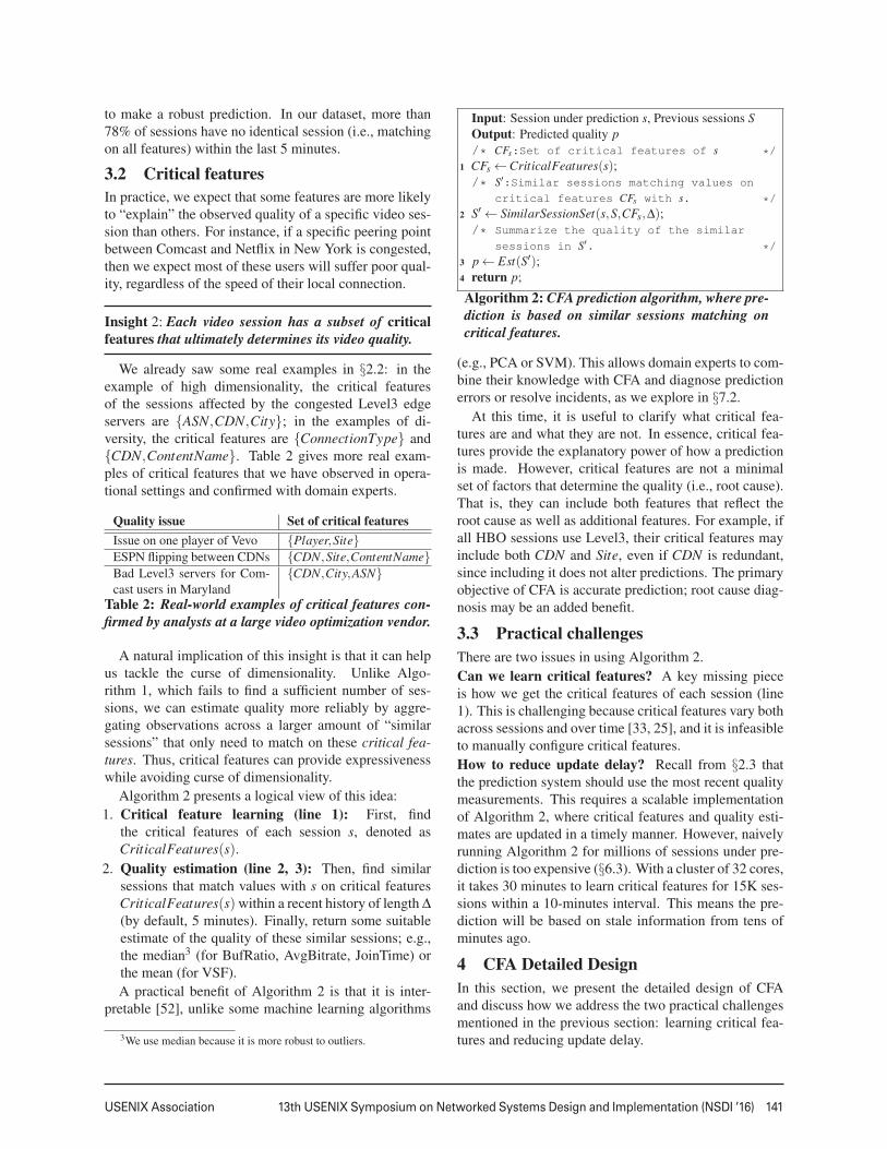
A natural implication of this insight is that it can helpus tackle the curse of dimensionality. Unlike Algo-rithm 1, which fails to find a sufficient number of ses-sions, we can estimate quality more reliably by aggre-gating observations across a larger amount of “similarsessions” that only need to match on these critical fea-tures. Thus, critical features can provide expressivenesswhile avoiding curse of dimensionality.

Algorithm 2 presents a logical view of this idea:1. Critical feature learning (line 1): First, find

the critical features of each session s, denoted asCriticalFeatures(s).

2. Quality estimation (line 2, 3): Then, find similarsessions that match values with s on critical featuresCriticalFeatures(s) within a recent history of length ∆(by default, 5 minutes). Finally, return some suitableestimate of the quality of these similar sessions; e.g.,the median3 (for BufRatio, AvgBitrate, JoinTime) orthe mean (for VSF).A practical benefit of Algorithm 2 is that it is inter-

pretable [52], unlike some machine learning algorithms

3We use median because it is more robust to outliers.

Input: Session under prediction s, Previous sessions SOutput: Predicted quality p/* CFs:Set of critical features of s */

1 CFs ←CriticalFeatures(s);/* S′:Similar sessions matching values on

critical features CFs with s. */2 S′ ← SimilarSessionSet(s,S,CFs,∆);/* Summarize the quality of the similar

sessions in S′. */3 p ← Est(S′);4 return p;

Algorithm 2: CFA prediction algorithm, where pre-diction is based on similar sessions matching oncritical features.

(e.g., PCA or SVM). This allows domain experts to com-bine their knowledge with CFA and diagnose predictionerrors or resolve incidents, as we explore in §7.2.

At this time, it is useful to clarify what critical fea-tures are and what they are not. In essence, critical fea-tures provide the explanatory power of how a predictionis made. However, critical features are not a minimalset of factors that determine the quality (i.e., root cause).That is, they can include both features that reflect theroot cause as well as additional features. For example, ifall HBO sessions use Level3, their critical features mayinclude both CDN and Site, even if CDN is redundant,since including it does not alter predictions. The primaryobjective of CFA is accurate prediction; root cause diag-nosis may be an added benefit.

3.3 Practical challengesThere are two issues in using Algorithm 2.Can we learn critical features? A key missing pieceis how we get the critical features of each session (line1). This is challenging because critical features vary bothacross sessions and over time [33, 25], and it is infeasibleto manually configure critical features.How to reduce update delay? Recall from §2.3 thatthe prediction system should use the most recent qualitymeasurements. This requires a scalable implementationof Algorithm 2, where critical features and quality esti-mates are updated in a timely manner. However, naivelyrunning Algorithm 2 for millions of sessions under pre-diction is too expensive (§6.3). With a cluster of 32 cores,it takes 30 minutes to learn critical features for 15K ses-sions within a 10-minutes interval. This means the pre-diction will be based on stale information from tens ofminutes ago.

4 CFA Detailed DesignIn this section, we present the detailed design of CFAand discuss how we address the two practical challengesmentioned in the previous section: learning critical fea-tures and reducing update delay.

5


Notations Domains Definitions,S,S A session, a set of ses-

sions, set of all sessionsq(s) S !→ R Quality of sQualityDist(S) 2S !→ 2R {q(s)|s ∈ S}f ,F,F A feature, a set of features,

set of all featuresCriticalFeatures(s) S !→ 2F Critical features of sV Set of all feature valuesFV ( f ,s) F×S !→ V Value on feature f of sFSV (F,s) 2F×S !→ 2V Set of values on features in

F of sSimilarSessionSet(s,S,F,∆)

F×2F×S×R+ !→ 2F

{s′|s′ ∈ S, t(s) − ∆ <t(s′) < t(s),FSV (F,s′) =FSV (F,s)}

Table 3: Notations used in learning of critical features.The key to addressing these challenges is our third and

final domain-specific insight:

Insight 3: Critical features tend to persist on longtimescales of tens of minutes.

This insight is derived from prior measurement stud-ies [25, 20]. For instance, our previous study on sheddinglight on video quality issues in the wild showed that thefactors that lead to poor video quality persist for hours,and sometimes even days [25]. Another recent studyfrom the C3 system suggests that the best CDN tends tobe relatively stable on the timescales of few tens of min-utes [20]. We independently confirm this observation in§6.3 that using slightly stale critical features (e.g., 30-60minutes ago) achieves similar prediction accuracy as us-ing the most up-to-date critical features. Though this in-sight holds for most cases, it is still possible (e.g., on mo-bile devices) that critical features persist on a relativelyshorter timescale (e.g., due to the nature of mobility).

Note that the persistence of critical features does notmean that quality values are equally persistent. In fact,persistence of critical features is on a timescale an orderof magnitude longer than the persistence of quality. Thatis, even if quality fluctuates rapidly, the critical featuresthat determine the quality do not change as often.

As we will see below, this persistence enables (a) au-tomatic learning of critical features from history, and (b)a scalable workflow that provides up-to-date estimates.

4.1 Learning critical featuresRecall that the first challenge is obtaining the critical fea-tures for each session. The persistence of critical featureshas a natural corollary that we can use to automaticallylearn them:

Corollary 3.1: Persistence implies that critical featuresof a session are learnable from history.

Specifically, we can simply look back over the his-tory and identify the subset of features F such thatthe quality distribution of sessions matching on F is

Input: Session under prediction s, Previous sessions SOutput: Critical features for s/* Initialization */

1 MaxSimilarity ←−∞,CriticalFeatures ← NULL;/* D f inest:Quality distribution of

sessions matching on F in ∆learn. */2 D f inest ← QualityDist(SimilarSessionSet(s,S,F,∆learn));3 for F ⊆ 2F do

/* Exclude F without enough similarsessions for prediction. */

4 if |SimilarSessionSet(s,S,F,∆)|< n then5 continue;

/* DF:Quality distribution ofsessions matching on F in ∆learn.

*/6 DF ← QualityDist(SimilarSessionSet(s,S,F,∆learn));

/* Get similarity of D f inest & DF. */7 Similarity ← Similarity(DF ,D f inest);8 if Similarity>MaxSimilarity then9 MaxSimilarity ← Similarity;

10 CriticalFeatures ← F ;11 return CriticalFeature;

Algorithm 3: Learning of critical features.

most similar to that of sessions matching on all fea-tures. For instance, suppose we have three features⟨ContentName,ASN,CDN⟩ and it turns out that sessionswith ASN = Comcast,CDN = Level3 consistently havehigh buffering over the last few hours due to some in-ternal congestion at the corresponding exchange point.Then, if we look back over the last few hours, thedata from history will naturally reveal that the dis-tribution of the quality of sessions with the featurevalues ⟨ContentName = Foo,ASN = Comcast,CDN =Level3⟩ will be similar to ⟨ContentName = ∗,ASN =Comcast,CDN = Level3⟩, but very different from, say,the quality of sessions in ⟨ContentName = ∗,ASN =∗,CDN = Level3⟩, or ⟨ContentName = ∗,ASN =Comcast,CDN = ∗⟩. Thus, we can use a data-drivenapproach to learn that ASN,CDN are the critical fea-tures for sessions matching ⟨ContentName=Foo,ASN =Comcast,CDN = Level3⟩.

Algorithm 3 formalizes this intuition for learning crit-ical features. Table 3 summarizes the notation used inAlgorithm 3. For each subset of features F (line 3), wecompute the similarity between the quality distribution(DF ) of sessions matching on F and the quality distri-bution (D f inest ) of sessions matching on all features (line7). Then, we find the F that yields the maximum sim-ilarity (line 8-10), under one additional constraint thatSimilarSessionSet(s,S,F,∆) should include enough (bydefault, at least 10) sessions to get reliable quality esti-mation (line 4-5). This check ensures that the algorithmwill not simply return the set of all features.

As an approximation of the duration in which criti-

6


��

��

��

� ��

��

��

��

� ��

��

��

�

��

� �

��

��

��

��

��

(a) Naive workflow (b) CFA workflow

��

��

Figure 5: To reduce update delay, we run criticalfeature learning and quality estimation at differenttimescales by leveraging persistence of critical features.cal features persist, we use ∆learn = 60min. Note that∆learn is an order of magnitude larger than the time win-dow ∆ used in quality estimation, because critical fea-tures persist on a much longer timescale than qualityvalues. We use (the negative of) Jensen-Shannon di-vergence between D1 and D2 to quantify their similaritySimilarity(D1,D2).

Although Algorithm 3 can handle most cases, thereare corner cases where SimilarSessionSet(s,S,F,∆learn)does not have enough sessions (i.e., more than n) to com-pute Similarity(DF ,D f inest) reliably. In these cases, wereplace D f inest by the set of n sessions that share mostfeatures with s over the time window of ∆learn. For-mally, we use {s′|s′ matches ks features with s}, whereks = argmink (|{s′|s′ matches k features with s|≥ n}|).

4.2 Using fresh updatesNext, we focus on reducing the update delay betweenwhen a quality measurement is received and used for pre-diction.

Naively running critical feature learning and qualityestimation of Algorithm 2 can be time-consuming, caus-ing the predictions to rely on stale data. In Figure 5(a),TCFL and TQE are the duration of critical feature learningand the duration of quality estimation, respectively. Thestaleness of quality estimation (depicted in Figure 5) torespond to a prediction query can be as large as the totaltime of two steps (i.e., TCFL + TQE ), which typically istens of minutes (§6.3). Also, simply using more parallelresources is not sufficient. The time to learn critical fea-tures using Algorithm 3 grows linearly with the numberof sessions under prediction, the number of history ses-sions, and the number of possible feature combinations.Thus, the complexity of learning critical features TCFL isexponential in the number of features. Given the currentset of features, TCFL is on the scale of tens of minutes.

To reduce update delay, we again leverage the persis-tence of critical features:

Corollary 3.2: Persistence implies that critical featurescan be cached and reused over tens of minutes.

Building on Corollary 3.2, we decouple the critical

feature learning and quality estimation steps, and runthem at separate timescales. On the timescale of tens ofminutes, we update the results of critical feature learn-ing. Then, on a faster timescale of tens of seconds, weupdate quality estimation using fresh data and the mostrecently learned critical features.

This decoupling minimizes the impact of staleness onprediction accuracy. Learning critical features on thetimescale of tens of minutes is sufficiently fast as theypersist on the same timescale. Meanwhile, quality esti-mation can be updated every tens of seconds and makespredictions based on quality updates with sufficientlylow staleness. Thus, the staleness of quality estimationTQE of the decoupled workflow (Figure 5(b)) is a magni-tude lower than TQE +TCFL of the naive workflow (Fig-ure 5(a)). In §6.3, we show that this workflow can retainthe freshness of critical features and quality estimates.

In addition, CFA has a natural property that two ses-sions sharing all feature values and occurring close intime will map to the same critical features. Thus, in-stead of running the steps per-session, we can reduce thecomputation to the granularity of finest partitions, i.e.,distinct values of all features.

4.3 Putting it togetherBuilding on these insights, we create the following prac-tical three-stage workflow of CFA.• Stage I: Critical feature learning (line 1 of Algo-

rithm 2) runs offline, say, every tens of minutes toan hour. The output of this stage is a key-value tablecalled critical feature function that maps all observedfinest partitions to their critical features.

• Stage II: Quality estimation (line 2,3 of Algo-rithm 2) runs every tens of seconds for all observedfinest partitions based on the most recent critical fea-tures learned in the first stage. This outputs anotherkey-value table called quality function that maps afinest partition to the quality estimation, by aggregat-ing the most recent sessions with the correspondingcritical features.

• Stage III: Real-time query/response. Finally, weprovide real-time query/response on the arrival of eachclient, operating at the millisecond timescale, by sim-ply looking up the most recent precomputed valuefunction from the previous stage. These operationsare simple and can be done very fast.Finally, instead of forcing all finest partition-level

computations to run in every batch, we can do triggeredrecomputations of critical feature learning only when theobserved prediction errors are high.

5 Implementation and DeploymentThis section presents our implementation of CFA andhighlights engineering solutions to address practical

7


��

��

��

��

��

��

�

��

��

��

Figure 6: Implementation overview of CFA. The threestages of CFA workflow are implemented in a backendcluster and distribute frontend clusters.challenges in operational settings (e.g., avoiding bulkdata loading and speeding up development iterations).

5.1 Implementation of CFA workflowCFA’s three stages are implemented in two different lo-cations: a centralized backend cluster and geographicallydistributed frontend clusters as depicted in Figure 6.Centralized backend: The critical feature learning andquality estimation stages are implemented in a backendcluster as periodic jobs. By default, critical feature learn-ing runs every 30 minutes, and quality estimation runsevery minute. A centralized backend is a natural choicebecause we need a global view of all quality measure-ments. The quality function, once updated by the estima-tion step, is disseminated to distributed frontend clustersusing Kafka [27].

Note that we can further reduce learning time usingsimple parallelization strategies. Specifically, the criti-cal features of different finest partitions can be learnedindependently. Similarly in Algorithm 3, the similarityof quality distributions can be computed in parallel. Toexploit this data-level parallelism, we implement them asSpark jobs [4].Distributed frontend: Real-time query/response anddecision makers of CDN/bitrate are co-located in dis-tributed frontend clusters that are closer to clients thanthe backend. Each frontend cluster receives the qualityfunction from the backend and caches it locally for fastprediction. This reduces the latency of making decisionsfor clients.

5.2 Challenges in an operational settingMitigating impact of bulk data loading: The backendcluster is shared and runs other delay-sensitive jobs; e.g.,analytics queries from production teams. Since the crit-ical feature learning runs periodically and loads a largeamount of data (≈30 GB), it creates spikes in the de-lays of other jobs (Figure 7). To address this concern,we engineered a simple heuristic to evenly spread thedata retrieval where we load a small piece of data everyfew minutes. As Figure 7 shows, this reduces the spikes

68 70 72 74 76 78 80 82 84

0 50 100 150 200 250 300 350 400

Avg

com

ple

tion tim

e

of back

gro

und jo

bs

(sec)

Time (min)

BatchSmooth

Figure 7: Streaming data loading has smoother impacton completion delay than batch data loading.

0

0.2

0.4

0.6

0.8

1

1.2

1.4

1.6

CFA NB DT k-NN LH ASN

Rela

tive e

rror

(a) AvgBitrate

0

0.5

1

1.5

2

2.5

3

3.5


Rela

tive e

rror

(b) JoinTime( ) g

0 20 40 60 80

100 120


Hit

Rat

e (%

)

Good Quality Bad Quality

(c) BufRatio

( )

0 20 40 60 80

100 120


Hit

Rat

e (%

)

Good Quality Bad Quality

(d) VSF

Figure 8: Distributions of relative prediction error({5,10,50,90,95}%iles) on AvgBitrate and JoinTimeand hit rates on BufRatio and VSF. They show thatCFA outperforms other algorithms.caused by bulk data loading in batch mode. Note that thisdoes not affect critical feature learning.Iterative algorithm refinement: Some parameters(e.g., learning window size ∆learn) of CFA require iter-ative tuning in a production environment. However, onepractical challenge is that the frontend-facing part of thebackend can only be updated once every couple of weeksdue to code release cycles. Thus, rolling out new predic-tion algorithms may take several days and is a practi-cal concern. Fortunately, the decoupling between criticalfeature learning and quality estimation (§4.2) means thatchanges to critical feature learning are confined to thebackend cluster. This enables us to rapidly refine andcustomize the CFA algorithm.

6 EvaluationIn this section, we show that:• CFA predicts video quality with 30% less error than

competing machine learning algorithms (§6.1).• Using CFA-based prediction, we can improve video

quality significantly; e.g., 32% less BufRatio, 12%higher AvgBitrate in a pilot deployment (§6.2).

• CFA is responsive to client queries and makes pre-dictions based on the most recent critical features andquality measurements (§6.3).

8


6.1 Prediction accuracyWe compare CFA with five alternative algorithms: threesimple ML algorithms, Naive Bayes (NB), Decision Tree(DT), k-Nearest Neighbor (k-NN)4, and two heuristicswhich predict a session’s quality by the average qualityof other sessions from the same ASN (ASN) or matchingthe last-mile connection type (LH). All algorithms usethe same set of features listed in Table 1.

Ideally, we want to evaluate how accurately an algo-rithm can predict the quality of a given client on everychoice of CDN and bitrate. However, this is infeasiblesince each video client is assigned to only one CDN andbitrate at any time. Thus, we can only evaluate the pre-diction accuracy over the observed CDN-bitrate choices,and we use the quality measured on these choices as theground truth. That said, this approach is still useful fordoing a relative comparison across different algorithms.

For AvgBitrate and JoinTime, we report relative error:|p−q|

q , where the q is the ground truth and p is the predic-tion. For BufRatio and JoinTime, which have more “stepfunction” like effects [18], we report a slightly differentmeasure called hit rate: how likely a session with goodquality (i.e., BufRatio < 5%, VSF=0) or bad quality iscorrectly identified. Figure 8 shows that for AvgBitrateand JoinTime, CFA has the lowest {5,10,50,90}%thpercentiles of prediction error and lower 95%th per-centiles than most algorithms. In particular, median er-ror of CFA is about 30% lower than the best competingalgorithm. In terms of BufRatio and VSF, CFA signifi-cantly outperforms other algorithms in the hit rate of badquality sessions. The reason for hit rate of bad qualityto be lower than that of good quality is that bad qualitysessions are almost always less than good quality, whichmakes them hard to predict. Note that accurately iden-tifying sessions that have bad quality is crucial as theyhave the most room for improvement.

6.2 Quality improvementPilot deployment: As a pilot deployment, we integratedCFA in a production system that provides a global videooptimization service [20]. We deployed CFA on one ma-jor content provider and used it to optimize 150,000 ses-sions each day. We ran an A/B test (where each algo-rithm was used on a random subset of clients) to evaluatethe improvement of CFA over a baseline random deci-sion maker, which many video optimization services useby default (modulo business arrangement like price) [9].

Table 4 compares CFA with the baseline random deci-sion maker in terms of the mean BufRatio, AvgBitrateand a simple QoE model (QoE = −370 ∗ Bu f Ratio +AvgBitrate/20), which was suggested by [33, 18]. Overall sessions in the A/B testing, CFA shows an improve-

4NB, DT, and k-NN are mplemented using a popular ML libraryweka[6].

CFA Baseline ImprovementQoE 155.43 138.27 12.4%BufRatio 0.0123 0.0182 32%AvgBitrate 3200 2849 12.31%

Table 4: Random A/B testing results of CFA vs. base-line in real-world deployment.

ment in both BufRatio (32% reduction) and AvgBitrate(12.3% increase) compared to the baseline. This showsthat CFA is able to simultaneously optimize multiple(possibly conflicting) metrics. To put these numbersin context, our conversation with domain experts con-firmed that these improvements are significant for con-tent providers and can potentially translate into substan-tial benefits in engagement and revenues [2]. CFA’s su-perior performance and that CFA is more automated thanthe custom algorithm indicate that domain experts werewilling to invest time running longer pilot. Figure 9 pro-vides more comparison and shows that CFA consistentlyoutperforms the baseline over time and across differentmajor cities in the US, connection types and CDNs.Trace-driven simulation: We complement this real-world deployment with a trace-driven simulation to si-multaneously compare more algorithms over more qual-ity metrics. However, one key challenge is that it is hardto estimate the quality of a decision that was not used bya specific client in the trace.

To address this problem, we use the counterfactualmethodology from prior work in online recommendationsystems [30, 31]. Suppose we have quality measure-ments from a set of clients, where client c is assigned toa decision drand(c) of CDN and bitrate at random. Now,we have a new hypothetical algorithm that maps clientc to dalg(c). Then, we can evaluate the average qualityof clients assigned to each decision d, {c|dalg(c) = d},by the average quality of {c|dalg(c) = d,drand(c) = d}.Finally, the average quality of the new algorithm is theweighted sum of average quality of all decisions, wherethe weight of each decision is the fraction of sessionsassigned to it. This can be proved to be an unbiased (of-fline) estimate of dalg’s (online) performance [5].5 Forinstance, if out of 1000 clients assigned to use Akamaiand 500Kbps, 200 clients are assigned to this decisionin the random assignment, then we can use the averagequality of these 200 sessions as an unbiased estimateof the average quality of these 1000 sessions. Fortu-nately, our dataset includes a (randomly chosen) portionof clients with randomized decision assignments (i.e.,

5One known limitation of this analysis is that it assumes the newassignments do not affect each decision’s overall performance. Forinstance, if we assign all sessions to one CDN, they may overload theCDN and so this CDN’s quality in the random assignments is no longeruseful. Since this work only focuses on controlling traffic at a smallscale relative to the total load on the CDN (and our experiments are infact performed at such a scale), this methodology is still unbiased.

9


60

80

100

120

140

160

180

0 5 10 15 20

QoE

Time (hour)

CFABaseline

(a) CFA vs. baseline by time

0

40

80

120

160

200

240

Level3Akamai

Amazon

QoE

CDNs

CFABaseline

0

40

80

120

160

200

240

CableDSL

MobileSatellite

Last hop connections

CFABaseline

0

40

80

120

160

200

240

280

LA NYCORL

CHISEA

Major US cities

CFABaseline

(b) CFA vs. baseline by spatial partitions

Figure 9: Results of real-world deployment. CFA outperforms the baseline random decision maker (over time andacross different large cities, connection types and CDNs).

0 10 20 30 40 50 60

QoE

BufRatio

AvgBitrate

JoinTime VSF

Impr

ovem

ent (

%) Over baseline

Over the best prediction algorithm

Figure 10: Comparison of quality improvement be-tween CFA and strawmen.

Stage Run time (mean/ median)

Requiredfreshness

Critical feature learning 30.1/29.5 min 30-60 minQuality estimation 30.7/28.5 sec 1-5 minQuery response 0.66/0.62 ms 1 ms

Table 5: Each stage of CFA is refreshed to meet therequired freshness of its results.

CDN and bitrate). Thus, we only report improvementsfor these clients.

Figure 10 uses this counterfactual methodology andcompares CFA with the best alternative from §6.1 foreach quality metric and the baseline random decisionmaker (e.g., the best alternative of AvgBitrate is k-NN).For each quality metric and prediction algorithm, the de-cision maker selects the CDN and bitrate that has the bestpredicted quality for each client. For instance, the im-provement of CFA over the baseline on VSF is 52% – thismeans the number of sessions with start failures is 52%less than when the baseline algorithm is used. The fig-ures show that CFA outperforms the baseline algorithmby 15%-52%. They also show that CFA outperforms thebest prediction algorithms by 5%-17%.

6.3 Timeliness of predictionOur implementation of CFA should (1) retain freshnessto minimize the impact of staleness on prediction accu-racy, and (2) be responsive to each prediction query.

We begin by showing how fast each stage describedin §4.2 needs to be refreshed. Figure 11 shows the im-pact of staleness of critical features and quality values

0

4

8

1 10 100

% in

cre

ase

in a

vg p

red

ictio

n e

rro

r

Staleness (min)

Critical featureQuality value

(a) BufRatio

0

4

8

12

1 10 100

% in

cre

ase

in a

vg p

red

ictio

n e

rro

r

Staleness (min)


(b) AvgBitrate

0

4

8

12

16

20

1 10 100

% in

cre

ase

in a

vg p

red

ictio

n e

rro

r

Staleness (min)


(c) JoinTime

4

8

12

16

20

24

1 10 100

% in

cre

ase

in a

vg p

red

ictio

n e

rro

r

Staleness (min)


(d) VSF

Figure 11: Latency of critical features and quality val-ues (x-axis) on increase in accuracy (y-axis).on the prediction accuracy of CFA. First, critical featureslearned 30-60 minutes before prediction can still achievesimilar accuracy as those learned 1 minute before predic-tion. In contrast, quality estimation cannot be more than10 minutes prior to when prediction is made (which cor-roborates the results of Figure 4(b)). Thus, critical fea-ture learning needs to be refreshed every 30-60 minutesand quality estimation should be refreshed at least everyseveral minutes. Finally, prediction queries need to beresponded to within several milliseconds [20] (ignoringnetwork delay between clients and servers).

Next, we benchmark the time to run each logical stagedescribed in §4.2. Real-time query/response runs in 4geographically distributed data centers. Critical featurelearning and quality estimation run on two clusters of 32cores. Table 5 shows the time for running each stage andthe timescale required to ensure freshness. It confirmsthat the implementation of CFA is sufficient to ensurethe freshness of results in each stage.

7 Insights from Critical FeaturesIn addition to the predictive power, CFA also offers in-sights into the “structure” of video quality in the wild. Inthis section, we focus on two questions: (1) What types

10


21%

21%

14% 10%

10%

24%

[ASN, City, CDN, ConnectionType] [ASN, City, CDN]

[ASN, City, CDN, Bitrate]

[ASN, CDN, Bitrate, ContentName] [Bitrate, ConnectionType, Player] Other

(a) BufRatio

17%

15%

15% 11%

9%

33%

[ASN, Bitrate, Player, ConnectionType] [City, CDN, Player, ConnectionType] [CDN, Bitrate]

[CDN, ConnectionType, Player] [ASN, City, CDN]

Other

(b) AvgBitrate

20%

14%

14% 12%

9%

31%

[ASN, CDN, Bitrate, ConnectionType] [Bitrate, ConnectionType]

[City, CDN, ConnectionType]

[CDN, ContentName, Bitrate] [CDN, Bitrate, Player]

Other

(c) JoinTime

]21%

20%

16% 11%

10%

22%

[ASN, CDN, ConnectionType] [City, CDN, ContentName]

[ASN, City, CDN, Bitrate]

[CDN, Bitrate, ConnectionType, Player] [ASN, CDN, ContentName]

Other

(d) VSF

Figure 12: Analyzing the types of critical features: Thisshows a breakdown of the total number of sessions as-signed to a specific type of critical features.of critical features are most common? (2) What factorshave significant impact on video quality?

7.1 Types of critical featuresPopular types of critical features: Figure 12 showsa breakdown of the fraction of sessions that are as-signed to a specific type of critical feature set. Weshow this for different quality metrics. (Since we fo-cus on a specific VoD provider, we do not consider theSite or LiveOrVoD for this analysis.) Across all qual-ity metrics, the most popular critical features are CDN,ASN and ConnectionType, which means video qualityis greatly impacted by network conditions at the server(CDN), transit network (ASN), and last-mile connection(ConnectionType).

We also see interesting patterns unique to individ-ual metrics. City is among the top critical features ofBufRatio. This is perhaps because network congestionusually depends on the volume of concurrent viewers ina specific region. Bitrate (initial bitrate) has a largerimpact on AvgBitrate than on other metrics, since thevideos in the dataset are mostly short content (2-5 min-utes) and AvgBitrate is correlated with initial bitrate. Fi-nally, ContentName has a relatively large impact on fail-ures (VSF) but not other metrics, because VSF is some-times due to the requested content not being ready.Distribution of types of critical features: While thequality of about 50% of sessions is impacted by 3-4 pop-ular types of critical features, 15% of sessions are im-pacted by a diverse set of more than 30 types of criticalfeature (not shown). This corroborates the need for ex-pressive prediction models that handle the diverse factorsaffecting quality (§2.2).

7.2 Values of critical featuresNext, we focus on the most prevalent feature values (e.g.,a specific ASN or player). To this end, we define preva-

City ASN Player ConnectionTypeBufRatio Some major

east-coastcities

Satellite,Mobile,Cable

AvgBitrate Cellularcarriers

Players withdifferent en-codings

JoinTime Cellularcarrier

Satellite,DSL

VSF SmallISPs

Satellite,Mobile

Table 6: Analysis of the most prevalent values of crit-ical features. A empty cell implies that we found nointeresting values in this combination.lence of a feature value by the fraction of video sessionsmatching this feature value that have this feature as oneof their critical features; e.g., the fraction of video ses-sions from Boston that have City as one of their criticalfeatures. If a feature value has a large prevalence, thenthe quality of many sessions that have this feature valuecan be explained by this feature.

We present the values of critical features with aprevalence higher than 50% for each quality metricand only consider a subset of the features (ASN, City,ContentName, ConnectionType) that appear promi-nently in Figure 12. We present this analysis with twocaveats. First, due to proprietary concerns, we do notpresent the names of the entities, but focus on their char-acteristics. Second, we cannot confirm some of our hy-pothesis as it involves other providers; as such, we intendthis result to be illustrative rather than conclusive.

Table 6 presents some anecdotal examples we ob-served. In terms of BufRatio, we see some of the majoreast coast cities (e.g., Boston, Baltimore) are more likelyto be critical feature values than other smaller cities. Wealso see both poor (Satellite, Mobile) and broadband (Ca-ble) connection types have high prevalence on BufRatioand JoinTime. This is because poor quality sessionsare bottlenecked by poor connections, while some goodquality sessions are explained by their broadband con-nections. “Player” has a relatively large prevalence onAvgBitrate, because the content provider uses differentbitrate levels for different players (Flash or iOS). Finally,in terms of VSF, some small ISPs have large prevalence.We speculate that this is because their peering relation-ships with major CDNs are not provisioned, so theirvideo sessions have relatively high failure rates.

8 Related WorkInternet video optimization: There is a large litera-ture on measuring video quality in the wild (e.g., contentpopularity [38, 55], quality issues [25] and server selec-tion [51, 47]) and techniques to improve user experience(e.g., bitrate adaptation algorithms [56, 26, 23], CDNoptimization and federation [32, 37, 11, 35] and cross-provider cooperation [57, 19, 24]). Our work builds on

11


insight from this prior work. While a case for a similarvision is made in [33], our work gives a systematic andpractical prediction system.Global coordination platform: Decision making basedon a global view is similar to other logically centralizedcontrol systems (e.g., [14, 33, 20, 48]). They examinedthe architectural issues of decoupling the control planefrom the data plane, including scalability (e.g., [50, 17]),fault tolerance (e.g., [36, 54]), and use of big data sys-tems (e.g., [20, 4]). In contrast, our work offers concretealgorithmic techniques over such a control platform [20]for video quality optimization.Large-scale data analytics in system design: Manystudies have applied data-driven techniques for perfor-mance diagnosis (e.g., [46, 15, 40]), revenue debugging(e.g., [13]), TCP throughput prediction (e.g., [22, 34]),and tuning TCP parameters (e.g., [43, 41]). Recent stud-ies try to operate these techniques at scale [16]. WhileCFA shares this data-driven approach, we exploit video-specific insights to achieve scalable and accurate predic-tion based on a global view of quality measurements.QoE models: Prior work has shown correlations be-tween various video quality metrics and user engagement(e.g., users are sensitive to BufRatio [18]), and built vari-ous QoE models (e.g., [28, 45, 12, 10]. Our work focuseson improving QoE by predicting individual quality met-rics, and can be combined with these QoE models.

9 DiscussionRelationship to existing ML techniques: CFA isa domain-specific prediction system that outperformssome canonical ML algorithms (§6.1). We put CFA inthe context of three types of ML algorithms.• Multi-armed bandit algorithms [53] find the decision

with the highest reward (i.e., best CDN and bitrate)from multiple choices. They assume each decision hasa fixed distribution of rewards, but the video quality ofa CDN also depends on client-side features. In con-trast, contextual multi-armed bandit algorithms [44]assume the best decision depends on contextual in-formation, but they require appropriate modeling be-tween the context and decision space, to which criticalfeatures provide one viable approach.

• The feature selection problem [21] seems similar tocritical feature learning, but with a key difference:critical features vary across video sessions. Thus,techniques looking for features that are most impor-tant for all sessions are not directly applicable.

• Advanced ML algorithms today can handle highlycomplex models [29, 42] efficiently, so in theory thecritical features could be automatically identified, al-beit in an implicit manner. CFA uses existing MLmodels (specifically, the “variable kernel conditionaldensity estimation” method [49]) and may be less ac-

curate than advanced ML techniques, but CFA canpredict with more recent data since it tolerates staleupdate on the critical features. Furthermore, CFA isless opaque since it is based on domain-specific in-sights about critical features (§7).

Finer grain information and selection: Currently,CFA makes predictions based on client side informationonly. While clients provide accurate information regard-ing QoE, prediction can be much more accurate if CFAwere to leverage finer-grained information from otherentities in the ecosystem, including servers, caches andnetwork paths. Furthermore, CFA currently selects re-sources at the CDN granularity. This means CFA cannotdo much if the CDN redirects the client based on its lo-cation and the servers the CDN redirects the client to arecongested. However, if the client were able to specifythe server to stream from, we could avoid the overloadedservers and improve quality.

10 ConclusionsMany prior research efforts posited that quality predic-tion could lead to improved QoE (e.g., [33, 11, 35, 10]).However, these efforts failed to provide a prescriptive so-lution that (a) is expressive enough to tackle the complexfeature-quality relationships observed in the wild and (b)can provide near real-time quality estimates. To this end,we developed CFA, a solution based on domain-specificinsights that video quality is typically determined by asubset of critical features which tend to be persistent.CFA leverages these insights to engineer an accurate al-gorithm that outperforms off-the-shelf machine learningapproaches and lends itself to a scalable implementationthat retains model freshness. Using real deployments andtrace-driven analyses, we showed that CFA achieves upto 30% improvement in prediction accuracy and 12-32%improvement in QoE over alternative approaches.

AcknowledgmentsThis paper would not be possible without the contribu-tion of Conviva Stuff, especially Jibin Zhan, Faisal Za-karia Siddiqi and Rui Zhang. The authors thank Sid-dhartha Sen for shepherding the paper and the NSDI re-viewers for their feedback. This research is supportedin part by NSF CISE Expeditions Award CCF-1139158,DOE Award SN10040 DE-SC0012463, and DARPAXData Award FA8750-12-2-0331, and gifts from Ama-zon Web Services, Google, IBM, SAP, The Thomas andStacey Siebel Foundation, Adatao, Adobe, Apple Inc.,Blue Goji, Bosch, Cisco, Cray, Cloudera, Ericsson, Face-book, Fujitsu, Guavus, HP, Huawei, Intel, Microsoft,Pivotal, Samsung, Schlumberger, Splunk, State Farm,Virdata and VMware. Junchen Jiang was supported inpart by NSF award CNS-1345305 and Juniper NetworksFellowship.

12


References[1] Conviva inc. http://www.conviva.com/.

[2] Personal communication with aditya ganjam from conviva, who is an experton video qoe.

[3] Quova. http://developer.quova.com/.

[4] Spark. http://spark.incubator.apache.org/.

[5] Technical note on counterfactual evaluation. https://www.cs.cmu.edu/cfe_technote.pdf.

[6] The weka manual 3.6.10. http://goo.gl/ISSY3c.

[7] Youtube and the olympics. http://goo.gl/4hgL4q.

[8] I. Sodagar. The MPEG-DASH Standard for Multimedia Streaming Overthe Internet. IEEE Multimedia, 2011.

[9] V. K. Adhikari, Y. Guo, F. Hao, V. Hilt, , and Z.-L. Zhang. A Tale of ThreeCDNs: An Active Measurement Study of Hulu and Its CDNs. In Proc.IEEE Global Internet Symposium, 2012.

[10] V. Aggarwal, E. Halepovic, J. Pang, S. Venkataraman, and H. Yan.Prometheus: toward quality-of-experience estimation for mobile apps frompassive network measurements. In Proceedings of the 15th Workshop onMobile Computing Systems and Applications, 2014.

[11] A. Balachandran, V. Sekar, A. Akella, and S. Seshan. Analyzing the poten-tial benefits of cdn augmentation strategies for internet video workloads. InACM IMC, pages 43–56, 2013.

[12] A. Balachandran, V. Sekar, A. Akella, S. Seshan, I. Stoica, and H. Zhang.Developing a predictive model of quality of experience for internet video.In ACM SIGCOMM ’13.

[13] R. Bhagwan, R. Kumar, R. Ramjee, G. Varghese, S. Mohapatra,H. Manoharan, and P. Shah. Adtributor: revenue debugging in advertis-ing systems. In USENIX NSDI, 2014.

[14] M. Caesar, D. Caldwell, N. Feamster, J. Rexford, A. Shaikh, and J. van derMerwe. Design and implementation of a routing control platform. InUSENIX NSDI 2005.

[15] D. R. Choffnes, F. E. Bustamante, and Z. Ge. Crowdsourcing service-levelnetwork event monitoring. In ACM SIGCOMM CCR, volume 40, pages387–398. ACM, 2010.

[16] D. Crankshaw, P. Bailis, J. E. Gonzalez, H. Li, Z. Zhang, M. J. Franklin,A. Ghodsi, and M. I. Jordan. The missing piece in complex analytics: Lowlatency, scalable model management and serving with velox. In Conferenceon Innovative Data Systems Research (CIDR), 2015.

[17] A. Dixit, F. Hao, S. Mukherjee, T. Lakshman, and R. Kompella. Towardsan elastic distributed sdn controller. In ACM HotSDN, 2013.

[18] F. Dobrian, V. Sekar, A. Awan, I. Stoica, D. A. Joseph, A. Ganjam, J. Zhan,and H. Zhang. Understanding the impact of video quality on user engage-ment. In Proc. SIGCOMM, 2011.

[19] B. Frank, I. Poese, Y. Lin, G. Smaragdakis, A. Feldmann, B. Maggs,J. Rake, S. Uhlig, and R. Weber. Pushing cdn-isp collaboration to the limit.ACM SIGCOMM CCR, 43(3), 2013.

[20] A. Ganjam, F. Siddiqi, J. Zhan, I. Stoica, J. Jiang, V. Sekar, and H. Zhang.C3: Internet-scale control plane for video quality optimization. In NSDI.USENIX, 2015.

[21] I. Guyon and A. Elisseeff. An introduction to variable and feature selection.The Journal of Machine Learning Research, 3:1157–1182, 2003.

[22] Q. He, C. Dovrolis, and M. Ammar. On the predictability of large transfertcp throughput. ACM SIGCOMM CCR, 35(4):145–156, 2005.

[23] T.-Y. Huang, R. Johari, N. McKeown, M. Trunnell, and M. Watson. Abuffer-based approach to rate adaptation: evidence from a large videostreaming service. In ACM SIGCOMM 2014.

[24] J. Jiang, X. Liu, V. Sekar, I. Stoica, and H. Zhang. Eona: Experience-oriented network architecture. In ACM HotNets, 2014.

[25] J. Jiang, V. Sekar, I. Stoica, and H. Zhang. Shedding light on the structureof internet video quality problems in the wild. In CoNEXT. ACM, 2013.

[26] J. Jiang, V. Sekar, and H. Zhang. Improving Fairness, Efficiency, and Sta-bility in HTTP-Based Adaptive Streaming with Festive . In ACM CoNEXT2012.

[27] J. Kreps, N. Narkhede, and J. Rao. Kafka: A distributed messaging systemfor log processing. In Proceedings of the NetDB, 2011.

[28] S. S. Krishnan and R. K. Sitaraman. Video stream quality impacts viewerbehavior: inferring causality using quasi-experimental designs. In IMC,2012.

[29] Y. LeCun, Y. Bengio, and G. Hinton. Deep learning. Nature,521(7553):436–444, 2015.

[30] L. Li, W. Chu, J. Langford, and R. E. Schapire. A contextual-bandit ap-proach to personalized news article recommendation. In Proceedings of the19th international conference on World wide web, pages 661–670. ACM,2010.

[31] L. Li, W. Chu, J. Langford, and X. Wang. Unbiased offline evaluation ofcontextual-bandit-based news article recommendation algorithms. In Pro-ceedings of the fourth ACM international conference on Web search anddata mining, pages 297–306. ACM, 2011.

[32] H. Liu, Y. Wang, Y. R. Yang, A. Tian, and H. Wang. Optimizing Cost andPerformance for Content Multihoming. In Proc. SIGCOMM, 2012.

[33] X. Liu, F. Dobrian, H. Milner, J. Jiang, V. Sekar, I. Stoica, and H. Zhang.A case for a coordinated internet video control plane. In ACM SIGCOMM,pages 359–370. ACM, 2012.

[34] M. Mirza, J. Sommers, P. Barford, and X. Zhu. A machine learning ap-proach to tcp throughput prediction. In ACM SIGMETRICS PerformanceEvaluation Review, volume 35, pages 97–108. ACM, 2007.

[35] M. K. Mukerjee, D. Naylor, J. Jiang, D. Han, S. Seshan, and H. Zhang.Practical, real-time centralized control for cdn-based live video delivery. InACM SIGCOMM, pages 311–324. ACM, 2015.

[36] A. Panda, C. Scott, A. Ghodsi, T. Koponen, and S. Shenker. Cap for net-works. In ACM HotSDN, 2013.

[37] L. Peterson and B. Davie. Framework for cdn interconnection. 2013.

[38] L. Plissonneau and E. Biersack. A longitudinal view of http video streamingperformance. In Proc. MMSys, 2012.

[39] W. B. Powell. Approximate Dynamic Programming: Solving the curses ofdimensionality, volume 703. John Wiley & Sons, 2007.

[40] R. R. Sambasivan, A. X. Zheng, M. De Rosa, E. Krevat, S. Whitman,M. Stroucken, W. Wang, L. Xu, and G. R. Ganger. Diagnosing perfor-mance changes by comparing request flows. In USENIX NSDI, 2011.

[41] S. Savage, N. Cardwell, and T. Anderson. The case for informed transportprotocols. In HotOS, pages 58–63. IEEE, 1999.

[42] B. Scholkopf and A. J. Smola. Learning with kernels: support vector ma-chines, regularization, optimization, and beyond. MIT press, 2002.

[43] S. Seshan, M. Stemm, and R. H. Katz. Spand: Shared passive networkperformance discovery. In USENIX Symposium on Internet Technologiesand Systems, pages 1–13, 1997.

[44] A. Slivkins. Contextual bandits with similarity information. The Journal ofMachine Learning Research, 15(1):2533–2568, 2014.

[45] H. H. Song, Z. Ge, A. Mahimkar, J. Wang, J. Yates, Y. Zhang, A. Basso,and M. Chen. Q-score: Proactive Service Quality Assessment in a LargeIPTV System. In Proc. IMC, 2011.

[46] M. Stemm, R. Katz, and S. Seshan. A network measurement architecturefor adaptive applications. In INFOCOM, volume 1, pages 285–294. IEEE,2000.

[47] A.-J. Su, D. R. Choffnes, A. Kuzmanovic, and F. E. Bustamante. Draftingbehind akamai (travelocity-based detouring). ACM SIGCOMM CCR, 2006.

13


[48] L. Suresh, M. Canini, S. Schmid, and A. Feldmann. C3: Cutting tail latencyin cloud data stores via adaptive replica selection. In USENIX NSDI, 2015.

[49] G. R. Terrell and D. W. Scott. Variable kernel density estimation. TheAnnals of Statistics, pages 1236–1265, 1992.

[50] A. Tootoonchian, S. Gorbunov, Y. Ganjali, M. Casado, and R. Sherwood.On controller performance in software-defined networks. In USENIX Work-shop on Hot Topics in Management of Internet, Cloud, and Enterprise Net-works and Services (Hot-ICE), 2012.

[51] R. Torres, A. Finamore, J. R. Kim, M. Mellia, M. M. Munafo, and S. Rao.Dissecting Video Server Selection Strategies in the YouTube CDN. InICDCS, 2011.

[52] A. Vellido, J. Martin-Guerroro, and P. Lisboa. Making machine learningmodels interpretable. In Proceedings of the 20th European Symposiumon Artificial Neural Networks, Computational Intelligence and MachineLearning (ESANN). Bruges, Belgium, pages 163–172, 2012.

[53] R. Weber et al. On the gittins index for multiarmed bandits. The Annals ofApplied Probability, 2(4):1024–1033, 1992.

[54] H. Yan, D. A. Maltz, T. E. Ng, H. Gogineni, H. Zhang, and Z. Cai. Tesser-act: A 4d network control plane. In NSDI, volume 7, pages 27–27, 2007.

[55] H. Yin et al. Inside the Bird’s Nest: Measurements of Large-Scale LiveVoD from the 2008 Olympics. In Proc. IMC, 2009.

[56] X. Yin, A. Jindal, V. Sekar, and B. Sinopoli. A control-theoretic approachfor dynamic adaptive video streaming over http. In SIGCOMM, pages 325–338. ACM, 2015.

[57] M. Yu, W. Jiang, H. Li, and I. Stoica. Tradeoffs in cdn designs for through-put oriented traffic. In CoNEXT, pages 145–156. ACM, 2012.

14

cfa: a practical prediction system for video qoe …junchenj/cfa.pdf · usenix association 13th...

Documents